A fully efficient time-parallelized quantum optimal control algorithm

Abstract

We present a time-parallelization method that enables to accelerate the computation of quantum optimal control algorithms. We show that this approach is approximately fully efficient when based on a gradient method as optimization solver: the computational time is approximately divided by the number of available processors. The control of spin systems, molecular orientation and Bose-Einstein condensates are used as illustrative examples to highlight the wide range of application of this numerical scheme.

I Introduction

The general goal of quantum control is to actively manipulate dynamical processes at the atomic or molecular scale D’Alessandro (2008); Brumer and Shapiro (2003). In recent years, the advances in quantum control have emerged through the introduction of appropriate and powerful tools coming from mathematical control theory and by the use of sophisticated experimental techniques to shape the corresponding control fields Brif et al. (2010); Glaser et al. (2015); Altafini and Ticozzi (2012); Dong and Petersen (2010). In this framework, different numerical optimal control algorithms Khaneja et al. (2005); Reich et al. (2012); Doria et al. (2011) have been developed and applied to a large variety of quantum systems. Optimal control was used in physical chemistry in order to steer chemical reactions Brif et al. (2010), but also for spin systems Levitt (2008); Ernst et al. (1987) with applications in Nuclear Magnetic Resonance Khaneja et al. (2005); Assémat et al. (2010); Lapert et al. (2012a, 2010); Khaneja et al. (2001); Zhang et al. (2011) and Magnetic Resonance Imaging Conolly et al. (1986); Bernstein et al. (2004); Lapert et al. (2012b). Recently, optimal control has attracted attention in view of applications to quantum information processing, for example as a tool to implement high-fidelity quantum gates in minimum time Glaser et al. (2015); Garon et al. (2013); Boozer (2012). Generally, algorithms can also be designed to account for experimental imperfections or constraints related to a specific material or device Glaser et al. (2015). The possibility of including such constraints renders optimal control theory more useful in view of experimental applications and helps bridge the gap between control theory and control experiments.

The standard numerical optimal control algorithms based on an iterative procedure compute the control fields through many time propagations of the state of the system, which can be prohibitive for systems of large dimensions in terms of computational time. This numerical limit can be bypassed by making use of parallel computing Toselli and Widlund (2005); Horton (1992); Maday et al. (2007). In the case the computational time is divided by the number of computers, the method is said to be fully efficient. This full efficiency can be viewed as the physical limit in terms of performance of a parallel algorithm. While in applied mathematics different techniques have been developed using space or time decomposition Toselli and Widlund (2005); Maday et al. (2007), very little has been done in quantum mechanics. The exponential growth of the Hilbert space dimension with the system size makes this question even more crucial in order to simulate the dynamics of complex quantum systems. Note that quantum control computations can also be speeded up by the parallelization of matrix exponential algorithms Gradl et al. (2006); Auckenthaler et al. (2010) and by parallelizing density operator time evolutions using minimal sets of pure states Skinner and Glaser (2002).

This paper is not aimed at proposing a new optimization approach, but rather at describing and studying a general framework, namely the Intermediate State Method (ISM), introduced in Maday et al. (2007), which uses a time-parallelization to speed up the computation of optimal control fields. We investigate the efficiency of ISM on three benchmark quantum control problems, ranging from the control of coupled spin systems and the control of molecular orientation to the control of Bose-Einstein condensates. As a by-product, we show under which conditions ISM can be made fully efficient.

The paper is organized as follows. Section II is dedicated to the description of the time-parallelization method. The numerical schemes involved in this algorithm are defined in Sec. III. Numerical results on the control of spin systems, molecular orientation and Bose-Einstein condensates are presented in Sec. IV. Conclusion and prospective views are given in Sec. V.

II The time-parallelization Method

We first introduce the optimal control problem and we derive the corresponding optimality conditions. We consider pure quantum states and we assume that the time evolution is coherent. Note that the formalism can be easily extended to mixed states or to the control of evolution operators Palao and Kosloff (2003). The control process is aimed at maximizing the transfer of population onto a target state, but modification of the algorithms in view of optimizing the expectation value of an observable is straightforward. The dynamics of the quantum system is governed by the Hamiltonian $\displaystyle H$. The initial and target states are denoted by $\displaystyle|\psi_{i}\rangle$ and $\displaystyle|\psi_{f}\rangle$, respectively and the general state of the system at time $\displaystyle t$, by $\displaystyle|\psi(t)\rangle$. The dynamics of the quantum system is governed by the Schrödinger equation:

$$i\partial_{t}|\psi(t)\rangle=H(u(t))|\psi(t)\rangle,$$ (1)

where $\displaystyle u(t)$ is the field to be determined. The control time $\displaystyle T$ is fixed. The objective of the control problem is to maximize the figure of merit $\displaystyle\mathcal{J}$

$$\mathcal{J}[u]=\Re[\langle\psi(T)|\psi_{f}\rangle]-\frac{\alpha}{2}\int_{0}^{T}u(t)^{2}dt,$$

$\displaystyle\alpha$ being a positive parameter which expresses the relative weight between the projection onto the target state and the energy of the control field. A necessary condition to ensure the optimality of $\displaystyle u$ is given by the cancellation of the gradient of $\displaystyle\mathcal{J}$ with respect to $\displaystyle u$ Khaneja et al. (2005):

$$\nabla\mathcal{J}[u](t)=-\alpha u(t)+\Im[\langle\chi(t)|\partial_{u(t)}H(u(t))|\psi(t)\rangle]=0,$$ (2)

where $\displaystyle|\chi(t)\rangle$ is the adjoint state that satisfies

$$i\partial_{t}|\chi(t)\rangle=H(u(t))|\chi(t)\rangle,$$ (3)

with the final condition $\displaystyle|\chi(t=T)\rangle=|\psi_{f}\rangle$.

We now present ISM. A schematic description is displayed in Fig. 1.

Figure 1: Schematic description of the Intermediate state method (see the text for details).

The main idea consists in considering a combination of the trajectories followed by $\displaystyle|\psi(t)\rangle$ and $\displaystyle|\chi(t)\rangle$ Salomon and Turinici (2006). Given $\displaystyle N\in\mathbb{N}$, we decompose the interval $\displaystyle[0,T]$ into a partition of sub-intervals $\displaystyle[0,T]=\cup_{n=0}^{N-1}[t_{n},t_{n+1}]$, with $\displaystyle 0=t_{0}<\cdots<t_{N}=T$. The parallelization strategy is based on this decomposition. We consider an arbitrary control $\displaystyle u$ and we introduce the sequence $\displaystyle|\varphi^{u}\rangle=(|\varphi^{u}_{n}\rangle)_{n=0,\cdots,N}$ that interpolates the state and adjoint state trajectories at time $\displaystyle t_{n}$ as follows:

$$|\varphi^{u}_{n}\rangle=\frac{T-t_{n}}{T}|\psi(t_{n})\rangle+\frac{t_{n}}{T}|\chi(t_{n})\rangle,$$ (4)

where $\displaystyle|\psi(t)\rangle$ and $\displaystyle|\chi(t)\rangle$ are defined by Eqs. (1) and (3), respectively. Note that $\displaystyle|\varphi^{u}\rangle$ does not sample any usual dynamics, e.g. $\displaystyle|\varphi^{u}\rangle$ does not correspond to a solution of Eq. (1). Its initial and final states are $\displaystyle|\varphi^{u}(0)\rangle=|\psi_{0}\rangle$ and $\displaystyle|\varphi^{u}(T)\rangle=|\psi_{f}\rangle$, respectively. The choice of intermediate states made in Eq. (4) is crucial to demonstrate Theorem 1 below Maday et al. (2007).

We then introduce in each sub-interval the optimal control problem $\displaystyle\max_{u_{n}}\mathcal{J}_{n}[|\varphi^{u}\rangle,u_{n}]$ defined by the maximization of the sub-functional:

$$\displaystyle\mathcal{J}_{n}[u_{n},|\varphi^{u}\rangle]=-\frac{1}{2}|||\psi_{n}(t_{n+1})\rangle-|\varphi_{n+1}^{u}\rangle||^{2}$$

$$\displaystyle-\frac{\alpha_{n}}{2}\int_{t_{n}}^{t_{n+1}}u_{n}(t)^{2}dt,$$

with $\displaystyle 0\leq n\leq N-1$. In this problem, the state $\displaystyle|\psi_{n}\rangle$ is defined on $\displaystyle[t_{n},t_{n+1}]$ by:

$$i\partial_{t}|\psi_{n}(t)\rangle=H(u(t))|\psi_{n}(t)\rangle,$$ (5)

starting from $\displaystyle|\psi_{n}(t_{n})\rangle=|\varphi^{u}_{n}\rangle$. The penalization coefficient is defined by $\displaystyle\alpha_{n}=\frac{t_{n+1}-t_{n}}{T}\alpha$. Since

$$\displaystyle\mathcal{J}_{n}[u_{n},|\varphi^{u}\rangle]=-\frac{1}{2}|||\psi_{n}(t_{n+1})\rangle||^{2}-\frac{1}{2}|||\varphi_{n+1}^{u}\rangle||^{2}$$

$$\displaystyle+\Re[\langle\psi_{n}(t_{n+1})|\varphi^{u}_{n+1}\rangle]-\frac{\alpha_{n}}{2}\int_{t_{n}}^{t_{n+1}}u_{n}(t)^{2}dt,$$

maximizing $\displaystyle\mathcal{J}_{n}$ with respect to $\displaystyle u$ is equivalent to maximize a figure of merit of the form: $\displaystyle\Re[\langle\psi_{n}(t_{n+1})|\varphi^{u}_{n+1}\rangle]-\frac{\alpha_{n}}{2}\int_{t_{n}}^{t_{n+1}}u_{n}(t)^{2}dt$. In this way, each sub-problem has the same structure as the initial one.

We now review some properties of the time decomposition in order to establish the relation with the original optimal control problem. Given an arbitrary trajectory $\displaystyle|\varphi(t)\rangle$, we define an auxiliary figure of merit:

$$\mathcal{J}_{\parallel}[u,|\varphi\rangle]=\sum_{n=0}^{N-1}\beta_{n}\mathcal{J}_{n}[u_{n},|\varphi\rangle],$$

with $\displaystyle\beta_{n}=\frac{T}{t_{n+1}-t_{n}}$. A first relation between $\displaystyle\mathcal{J}_{\parallel}$ and $\displaystyle\mathcal{J}$ is given in Theorem 1 (see Ref. Maday et al. (2007) for the proof).

Theorem 1.

Given an arbitrary control $\displaystyle u$, we have:

$$|\varphi^{u}\rangle={\rm argmax}_{|\varphi\rangle}\big{(}\mathcal{J}_{\parallel}[u,|\varphi\rangle]\big{)}.$$

Moreover, the following relation is satisfied:

$$\mathcal{J}_{\parallel}[u,|\varphi^{u}\rangle]=\mathcal{J}[u].$$

As a by-product, this Theorem allows us to compute in parallel $\displaystyle\mathcal{J}[u]$, knowing only the sequence $\displaystyle|\varphi_{u}\rangle$. A similar relation also holds between the gradients of the functionals, as stated in Theorem 2.

Theorem 2.

Given an arbitrary control $\displaystyle u$, we have:

$$\nabla\mathcal{J}[{u}]_{|[t_{n},t_{n+1}]}=\beta_{n}\nabla\mathcal{J}_{n}[{u_{|[t_{n},t_{n+1}]}},|\varphi^{u}\rangle].$$

This result provides a new interpretation of the time-parallelized method since the sequence $\displaystyle|\varphi^{u}(t_{n})\rangle$, $\displaystyle n=0,\cdots,N$ of intermediate states enables the decomposition of the computation of the gradient.

Proof: Let us consider a fixed value $\displaystyle n$, with $\displaystyle 0\leq n\leq N-1$, $\displaystyle t\in[t_{n},t_{n+1}]$ and denote by $\displaystyle|\chi_{n}(t)\rangle$ and $\displaystyle|\psi_{n}(t)\rangle$ the trajectories defined by

$$i\partial_{t}|\chi_{n}(t)\rangle=H(u(t))|\chi_{n}(t)\rangle,$$

and

$$i\partial_{t}|\psi_{n}(t)\rangle=H(u(t))|\psi_{n}(t)\rangle,$$

with $\displaystyle|\chi_{n}(t_{n+1})\rangle=|\varphi^{u}_{n+1}\rangle$ and $\displaystyle|\psi_{n}(t_{n})\rangle=|\varphi^{u}_{n}\rangle$. For $\displaystyle t\in[t_{n},t_{n+1}]$, we repeat with $\displaystyle\mathcal{J}_{n}$ the computation made to derive the gradient of $\displaystyle\mathcal{J}$:

$$\displaystyle\nabla\mathcal{J}_{n}[u_{|[t_{n},t_{n+1}]},|\varphi^{u}\rangle](t) \displaystyle= \displaystyle\Im\left(\langle\chi_{n}(t)|\partial_{u(t)}H|\psi_{n}(t)\rangle\right)$$

$$\displaystyle-\alpha_{n}u(t).$$

Using the fact that:

$$|\chi_{n}(t)\rangle=\frac{(T-t_{n+1})}{T}|\psi(t)\rangle+\frac{t_{n+1}}{T}|\chi(t)\rangle,$$

and

$$|\psi_{n}(t)\rangle=\frac{(T-t_{n})}{T}|\psi(t)\rangle+\frac{t_{n}}{T}|\chi(t)\rangle,$$

we arrive at:

$$\displaystyle\nabla\mathcal{J}_{n}[u_{|[t_{n},t_{n+1}]},|\varphi^{u}\rangle](t) \displaystyle= \displaystyle\frac{1}{\beta_{n}}\Im\left(\langle\chi(t)|\partial_{u(t)}H|\psi(t)\rangle\right)$$

$$\displaystyle-\frac{\alpha}{\beta_{n}}u(t),$$

and the result follows.$\displaystyle\Box$

We now give the general structure of ISM. Let $\displaystyle 1\geq\eta>0$ and $\displaystyle u^{(0)}$ be an initial control field.

Algorithm 1.

1. Set $\displaystyle Err=1$, $\displaystyle k=0$.

2. While $\displaystyle Err>\eta$, do:
   

   1. Compute on $\displaystyle[0,T]$ the trajectories $\displaystyle|\psi^{(k)}(t)\rangle$ and $\displaystyle|\chi^{(k)}(t)\rangle$ associated with $\displaystyle u^{(k)}$ according to Eqs. (1) and (3).

   2. Compute $\displaystyle|\varphi^{(k)}(t)\rangle=|\varphi^{u^{(k)}}(t)\rangle$ according to Eq. (4).

   3. On each sub-interval $\displaystyle[t_{n},t_{n+1}]$ compute in parallel an approximation of the solution $\displaystyle u^{(k+1)}_{n}$ of the problem $\displaystyle\max_{u_{n}}\mathcal{J}_{n}[u_{n},|\varphi_{k}\rangle]$.

   4. Define $\displaystyle u^{(k+1)}$ as the concatenation of the controls $\displaystyle u^{(k+1)}_{n}$, $\displaystyle n=1,\cdots,N-1$.

   5. Set $\displaystyle Err=\sum_{n=0}^{N-1}\int_{T_{n}}^{T_{n+1}}\|\nabla\mathcal{J}_{n}[u^{(k+1)}_{|[t_{n},t_{n+1}]}](t)\|dt$.

   6. Set $\displaystyle k=k+1$.

Step 2a contradicts the parallelization paradigm, since it requires a sequential solving of an evolution equation on the full interval $\displaystyle[0,T]$. We will see how this problem can be solved in Sec. IV. However, note that the most time consuming step, namely Step 2c, is achieved in parallel.

III Description of the numerical methods used in the parallelization

Different schemes can be used to implement the time-parallelized algorithm in practice. This requires two ingredients, a numerical scheme to solve approximately the evolution equations of Steps 2a and 2c and an optimization procedure for the sub-problem of Step 2c. In this paragraph, we give some details about the used numerical methods and we explain how the full efficiency can be approached in the case of quantum systems of sufficiently small dimensions.

In the different numerical examples, we consider two numerical solvers for the Schrödinger Equation (1): a Crank-Nicholson scheme and a second order Strang operator splitting. Such solvers can be described through an equidistant time-discretization grid $\displaystyle t_{a}=t_{0}<t_{1}<\cdots<t_{J}=t_{b}$ of an interval $\displaystyle[t_{a},t_{b}]$. The time step is denoted by $\displaystyle\tau=(t_{b}-t_{a})/(J-1)$ for some $\displaystyle J\in\mathbb{N}$. For each time grid point $\displaystyle t_{j}$, we introduce the state $\displaystyle|{\psi}_{j}\rangle$ and the control $\displaystyle u_{j}$, which are some approximations of the exact state $\displaystyle|\psi(t_{j})\rangle$ and of the exact control field $\displaystyle u(\frac{t_{j}+t_{j+1}}{2})$.

The Crank-Nicholson algorithm is based on the following recursive relation:

$$\frac{i}{\tau}(|{\psi}_{j+1}\rangle-|{\psi}_{j}\rangle)=\frac{H(u_{j})}{2}(|{\psi}_{j+1}\rangle+|{\psi}_{j}\rangle),$$ (6)

which can be rewritten in a more compact form as

$$(Id+L_{j})|\psi_{j+1}\rangle=\big{(}Id-L_{j}\big{)}|\psi_{j}\rangle\,,$$ (7)

where $\displaystyle Id$ is the identity operator and $\displaystyle L_{n}:=i\frac{\tau}{2}H(u_{n}(t))$.

The second order Strang operator splitting is rather used in the case of infinite dimensional systems. Indeed, this method is particularly relevant when the Hamiltonian includes a differential operator. We consider, for example, the case $\displaystyle H(u(t))=-\Delta+V(u(t),x)$ where $\displaystyle\Delta$ denotes the Laplace operator and $\displaystyle V(u(t))=V(u(t),x)$ is a scalar potential. In this case, Strang’s method gives rise to the iteration:

$$|{\psi}_{j+1}\rangle=\exp(-\frac{i\tau}{2}\Delta)\exp(-i\tau V(u_{j}))\exp(-\frac{i\tau}{2}\Delta)|{\psi}_{j}\rangle.$$ (8)

In Eq. (8), each product can be determined very quickly since the operator $\displaystyle V(u_{j})$ is diagonal in the physical space, while $\displaystyle\Delta$ is generally diagonal in the Fourier space, and the change of basis can be achieved efficiently by fast Fourier transform.

These schemes provide a second order approximation with respect to time, which leads to an accurate approximation of the trajectory $\displaystyle|\psi(t)\rangle$. In addition, both propagators automatically preserve the normalization of the wave function, which is very interesting to avoid non-physical solutions. A specific advantage of these solvers is that they allow an exact differentiation with respect to the control in the discrete setting, in the case of scalar control for the Strang solver (8) and in any case for the Crank-Nicholson solver (6).

We now explain how the full efficiency can be reached with the parallelization algorithm. Both solvers lead to a linear relation between the initial and the final states of the system of the form:

$$|{\psi}_{J}\rangle=M(u)|{\psi}_{0}\rangle.$$

As an example, for the Crank-Nicholson solver, we have:

$$~{}M(u)=\Pi_{j=0}^{J-1}(Id+L_{j})^{-1}(Id-L_{j}).$$

The matrix $\displaystyle M(u)$ can be computed in parallel during the propagation of Eq. (7). Knowing the state $\displaystyle|{\psi}_{0}\rangle$, this matrix enables to compute in one matrix-vector product $\displaystyle|{\psi}_{J}\rangle$. As a consequence, this propagator assembling technique allows us to avoid the sequential solving on the full interval $\displaystyle[0,T]$ in Step 2a of Algorithm 1. More precisely, assume for example that at iteration $\displaystyle k$ of Algorithm 1 and on each sub-interval, a matrix $\displaystyle M_{n}(u^{(k)}_{n})$ is computed and transmitted to the main processor. The computations of the sequences $\displaystyle|\psi(t_{n})\rangle$ and $\displaystyle|\chi(t_{n})\rangle$, that are required to define the intermediate states $\displaystyle|\varphi^{(k)}(t_{n})\rangle$, can be achieved in $\displaystyle 2N$ matrix-vector products. Due to storage and communications issues of the matrices, note that this approach can only be used for quantum systems of small dimensions.

We conclude this paragraph by presenting a way to derive the gradient of time-discretized figures of merit of the form:

$$\mathcal{J}_{\tau}[u]=\Re\langle{\psi}_{J}|\psi_{f}\rangle-\frac{\alpha}{2}\tau\sum_{j=0}^{J-1}u_{j}^{2}.$$

We consider the case of a Crank-Nicholson solver, but similar computations can be made for Strang’s solver. We introduce the functional $\displaystyle\L_{\tau}$ defined by:

$$\displaystyle\L_{\tau}[u,|\psi\rangle,|\chi\rangle]=\mathcal{J}_{\tau}[u]+\Re(\sum_{j=0}^{J-1}\langle\chi_{j}|Id+L_{j}|\psi_{j+1}\rangle$$

$$\displaystyle-\langle\chi_{j}|Id-L_{j}|\psi_{j}\rangle).$$

Since $\displaystyle L_{j}$ is anti-hermitian, differentiating $\displaystyle\L_{\tau}$ with respect to $\displaystyle|\psi\rangle$ gives rise to the discrete adjoint evolution equation:

$$(Id-L_{j-1})|\chi_{j-1}\rangle=(Id+L_{j})|\chi_{j}\rangle,$$

with the final condition $\displaystyle(Id-L_{J-1})|\chi_{J-1}\rangle=|\psi_{J}\rangle$. To derive the gradient of $\displaystyle\mathcal{J}_{\tau}[u]$, it remains to differentiate $\displaystyle L_{\tau}$ with respect to $\displaystyle u$, which leads to the $\displaystyle j$-th entry of the gradient of $\displaystyle\mathcal{J}_{\tau}$:

$$\left(\nabla\mathcal{J}_{\tau}[u]\right)_{j}=\alpha dtu_{j}+\frac{i\tau}{2}\langle\chi_{j}|\partial_{u}H|\psi_{j+1}+\psi_{j}\rangle.$$

In the sequel, we use this result to implement a constant step gradient method: the approximation of the solution of the sub-problem in Step 2d is computed by iterating on $\displaystyle\ell$ in the formula:

$$u^{\ell+1}=u^{\ell}-\rho\nabla\mathcal{J}_{\tau}(u^{\ell}),$$ (9)

for some $\displaystyle\rho>0$.

Other optimization methods such as pseudo or quasi-Newton approaches can be used to perform Step 2c.

IV Numerical results

This section is dedicated to some numerical results obtained with ISM, used with the schemes presented in Sec. III. The efficiency of this approach is illustrated on three benchmark examples in quantum control Brif et al. (2010); Glaser et al. (2015), namely the control of a system of coupled spins, the control of molecular orientation and the control of a Bose-Einstein condensate whose dynamics is governed by the Gross-Pitaevskii equation.

IV.1 Control of a system of five coupled spins

In this paragraph, we consider the control of a system of coupled spin 1/2 particles. The principles of control in Nuclear Magnetic Resonance being described in different books Bernstein et al. (2004); Ernst et al. (1987); Levitt (2008), only a brief account will be given here in order to introduce the used model. We investigate the control of a system of coupled spins by means of different magnetic fields acting as local controls on each spin. Each field only acts on one spin and does not interact with the others, i.e. the spins are assumed to be selectively addressable.

We introduce a system of 5 coupled spins Marx et al. (2000, 2015), the evolution of which is described by the following Hamiltonian:

$$H=H_{0}+\sum_{k=1}^{5}[u_{x}^{k}(t)I_{x}^{(k)}+u_{y}^{k}(t)I_{y}^{(k)}]$$ (10)

where the operators $\displaystyle I_{x}^{(k)}$ and $\displaystyle I_{y}^{(k)}$ are, up to a factor, Pauli matrices which only act on the $\displaystyle k$th spin:

$$I_{x}:=\left(\begin{array}[]{cc}0&1/2\\ 1/2&0\end{array}\right),I_{y}:=\left(\begin{array}[]{cc}0&-i/2\\ i/2&0\end{array}\right),$$

$$I_{z}:=\left(\begin{array}[]{cc}1/2&0\\ 0&-1/2\end{array}\right).$$

We assume that the free evolution Hamiltonian $\displaystyle H_{0}$ is associated with a topology Marx et al. (2000, 2015) defined by:

$$\displaystyle H_{0}=2\pi(J_{12}I_{z}^{(1)}I_{z}^{(2)}+J_{13}I_{z}^{(1)}I_{z}^{(3)}+$$

$$\displaystyle+J_{23}I_{z}^{(2)}I_{z}^{(3)}+J_{25}I_{z}^{(2)}I_{z}^{(5)}+J_{34}I_{z}^{(3)}I_{z}^{(4)}).$$

Note that this model system is valid in heteronuclear spin systems if the coupling strength between the spins is small with respect to the frequency shifts Ernst et al. (1987); Levitt (2008). The coupling constant between the spins is taken to be uniform and equal to $\displaystyle J_{p}=140$. For the numerical simulations, we move to the density matrix formalism with $\displaystyle I_{x}^{(1)}$ and $\displaystyle I_{x}^{(5)}$ as initial and final states, respectively. The control time is fixed to $\displaystyle T=J_{p}/10$. The parameter $\displaystyle\alpha$ is set to 0.

For the time-parallelization, we consider a uniform grid, so that $\displaystyle t_{n+1}-t_{n}=T/N$, for $\displaystyle n=0,\cdots,N-1$ and we compare the results for different values of $\displaystyle N$. The time discretization is done by the Crank-Nicholson method of Eq. (6) with the time step $\displaystyle T/2^{15}$. In Step 2c, one iteration of the constant step gradient descent method [see Eq. (9)] is used, with $\displaystyle\rho=10^{4}$. As a result of Theorem 2, the values obtained after a given number of iterations are the same for all values of $\displaystyle N$. In this way, the method is almost fully efficient. It is actually equivalent to a standard gradient method, except that the computation of the gradient is done in parallel. The computational effort is therefore exactly divided by the number of processors, and the full efficiency is only limited by the memory usage and also by the communication between processors required by the update of the intermediate states in Steps 2a and 2b of the algorithm. Figure 2 displays the figure of merit with respect to the parallel computational time.

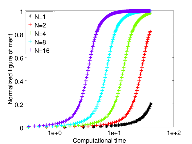
Figure 2: Evolution of the normalized figure of merit at each iteration and for different values of $\displaystyle N$ (the number of processors) with respect to computational time (wall-clock time) in the case of the control of a spin system. As stated in Theorem 2, the values obtained after a given number of iterations are the same for all values of $\displaystyle N$. Log-scale is used in the x-axis.

In order to evaluate more precisely the efficiency of the algorithm, we give some details about the speedup of the numerical computations. Numerical simulations are implemented with Matlab, where the parallelization is realized using the open source library MatlabMPI Kepner and Ahalt (2004a). The tests have been carried out on a shared memory machine under a linux system with a core of Intel(R) Xeon(R) CPU type (@ 2.90GHz with 198 Giga byte shared memory). The parallel computation uses $\displaystyle N$ processors where $\displaystyle N$ stands, as above, for the number of sub-intervals of the time domain decomposition. In Fig. 3, parallel numerical performances are compared with the sequential performance which is obtained when a single processor is used to treat the whole time domain. Given $\displaystyle\varepsilon>0$, we introduce the quantities $\displaystyle S(\varepsilon,N):={t(\varepsilon,1)}/{t(\varepsilon,N)}$ and $\displaystyle Eff(\varepsilon,N):=10^{2}({S(\varepsilon,N)}/{N}),$ as the parallel speedup and the efficiency respectively, where $\displaystyle t(\varepsilon,N)$ denotes the computational time (with $\displaystyle N$ processors) necessary to reach a value $\displaystyle\mathcal{J}[u^{k}]$ such that $\displaystyle\mathcal{J}[u^{\infty}]-\mathcal{J}[u^{k}]<\varepsilon$, where $\displaystyle u^{\infty}$ is the value of the sequence $\displaystyle u^{k}$ obtained at the numerical convergence. Figure 3 displays results about the speedup of the parallel implementation.

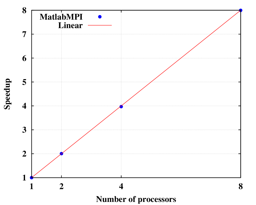
Figure 3: Speedup $\displaystyle S(1.74,N)$ of the parallel implementation (y- axis) with respect to the number of processors $\displaystyle N$ (x- axis). The blue dots indicate the speedup achieved with MatlabMPI for $\displaystyle\varepsilon=1.74$ (see Table 1 for details). The red solid line corresponds to a linear evolution of the speedup as a function of $\displaystyle N$.

We observe that the algorithm behaves as expected when increasing the number of processors. Despite the use of Input/Output (I/O) data files to ensure the communication between CPUs (as required by MatlabMPI), ISM achieves a linear scalability. A profiling of the parallel computing is reported in Fig. 4 where we present the time spent to achieve the communications for the master and one slave processors during 20 iterations of the optimization process. As expected, the speedup is independent on the value of $\displaystyle\varepsilon$. This point is clearly exhibited in Table 1. The communications in MatlabMPI are of point-to-point type through I/O files, a for-loop is therefore necessary to cover all sender and receiver processors. In this view, a slave processor waits for its turn in order to be able to read the message from the master processor. On the contrary, the printing message addressed to the master processor is done on slave processors and hence is non-blocking.

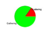
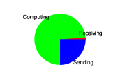
Master processor	Slave processor

Figure 4: MPI profiling of the tasks performed by the master and a slave processors with $\displaystyle N=4$ and for 20 iterations of the optimization process. The proportions are computed separately regarding the own wall-clock timing of a given processor.

Figure 4 shows that, in the case $\displaystyle N=4$, the slave processor mainly works on parallel computing. Its communication part is shared between sending and receiving data. The sending part is longer due to the amount of data to treat, which consists not only of partial control but also of propagator matrices.

$\displaystyle N$ processors	1	2	4	8
$\displaystyle Eff(0.32,N)$	100%	100.5%	99.7 %	100.9%
$\displaystyle Eff(0.89,N)$	100%	100.2 %	99.2 %	99.9%
$\displaystyle Eff(1.74,N)$	100%	100.2%	99.2%	99.9%

Table 1: Efficiency $\displaystyle Eff(\varepsilon,N)$ of the parallel MPI implementation. Note the full efficiency performance through several snapshots in the running parallel computing.

The full efficiency of ISM is clearly shown in the numerical simulations, see Table. 1. Note that, in some cases, the efficiency is greater than $\displaystyle 100\%$ because the full problem requires more memory, and thus spends more time in hardware storage processes. On the contrary, the parallel computing uses a smaller amount of data. Also, depending on the processor architecture, the computational time shall behave nonlinearly with respect to the size of the data. Similar linear and super linear speedup have been observed in Ref. Kepner and Ahalt (2004b) with MatlabMPI.

IV.2 Optimal control of molecular orientation

In a second series of numerical tests, we consider the control of molecular orientation by THz laser fields. Molecular orientation Stapelfeldt and Seideman (2003); Seideman and Hamilton (2006) is nowadays a well-established topic both from the experimental Znakovskaya et al. (2009); Fleischer et al. (2011) and theoretical points of views Dion et al. (2001); Averbukh and Arvieu (2001); Daems et al. (2005); Lapert and Sugny (2012); Tehini and Sugny (2008). Different optimal control analyses have been made on this quantum system Salomon et al. (2005); Lapert et al. (2008); Yoshida and Ohtsuki (2014); Nakajima et al. (2012).

In this paragraph, we consider the control of a linear polar molecule, HCN, by a linearly polarized THz laser field $\displaystyle E(t)$. We assume that the molecule is in its ground vibronic state and described by a rigid rotor. In this case, the Hamiltonian of the system can be written as:

$$H(t)=BJ^{2}-\mu_{0}\cos\theta E(t)-\frac{E(t)^{2}}{2}[(\alpha_{\parallel}-\alpha_{\perp})\cos^{2}\theta+\alpha_{\perp}],$$

where $\displaystyle B$ is the rotational constant, $\displaystyle J^{2}$ the angular momentum operator, $\displaystyle\mu_{0}$ the permanent dipolar moment, $\displaystyle\alpha_{\parallel}$ and $\displaystyle\alpha_{\perp}$ the dipole polarizability components parallel and perpendicular to the molecular axis, respectively, and $\displaystyle\theta$ the angle between the molecular axis and the polarization direction of the electric field. At zero temperature, the dynamics of the system is ruled by the following differential equation:

$$i\frac{\partial|\psi(t)\rangle}{\partial t}=H(t)|\psi(t)\rangle$$

where the initial state at $\displaystyle t=0$ is $\displaystyle|0,0\rangle$, in the basis of the spherical harmonics $\displaystyle\{|j,m\rangle,~{}j\geq 0,~{}-j\leq m\leq j\}$. Numerical values are taken to be $\displaystyle B=6.6376\times 10^{−6}$, $\displaystyle\mu_{0}=1.1413$, $\displaystyle\alpha_{\parallel}=20.055$ and $\displaystyle\alpha_{\perp}=8.638$, in a.u. We refer the reader to Ref. Salomon et al. (2005) for details on the numerical implementation of this control problem. The $\displaystyle\alpha$ parameter is chosen as a time-dependent function of the form $\displaystyle 10^{5}(\frac{t-T/2}{T/2})^{6}+10^{4}$ in order to design a control field which is experimentally relevant Salomon et al. (2005). The target state is the eigenvector of the observable $\displaystyle\cos\theta$ with the maximum eigenvalue in the subspace such that $\displaystyle j\leq 4$ Daems et al. (2005); Sugny et al. (2005).

Having investigated the implementation issues in Sec. IV.1, we focus in this paragraph on the efficiency $\displaystyle Eff^{\star}(\varepsilon,N)$ achieved when neglecting the time associated with I/O communications. As a consequence, the results hereafter do not depend on the used computer and software. We study the efficiency of the parallelization method in the cases where the optimization solver consists in one step of either a monotonic algorithm or a Newton method. We start with a simulation using monotonic algorithm (see Salomon (2007); Reich et al. (2012) for details about this method). Given a target value $\displaystyle\varepsilon$ of the figure of merit, we measure the computational time necessary to obtain it. In the numerical computation, we use $\displaystyle\varepsilon=0.3$, while the optimum has been numerically estimated as $\displaystyle 0.2909$ Salomon et al. (2005). The values of the figure of merit are plotted in Fig. 5.

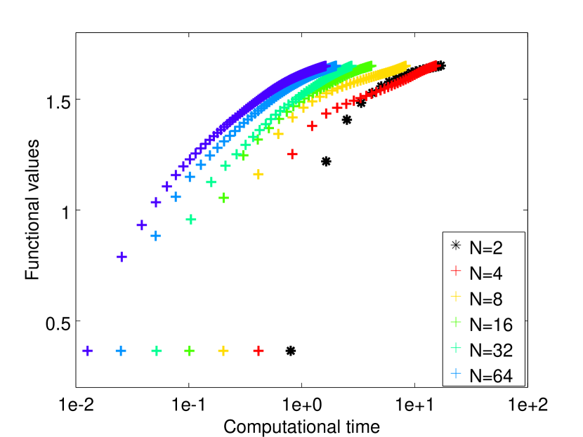
Figure 5: Functional values at each iteration and for various values of $\displaystyle N$ with respect to computational time for the control of molecular orientation by a monotonic algorithm. Log-scale is used in the x-axis.

In this case, the full efficiency is not obtained, as reported in Table 2.

$\displaystyle N$	$\displaystyle Eff^{\star}(\varepsilon,N)$
1	100%
2	55.2%
4	51.2%
8	51.5%
16	38.5%
32	26.4%
64	16.3%

Table 2: Efficiency of ISM for various values of $\displaystyle N$ in the case of the control of molecular orientation with a monotonic algorithm.

In the different numerical simulations, we observe that this method seems to be significantly more efficient than gradient descent solvers. The wall-clock computational time is a decreasing function of $\displaystyle N$, so that solving benefits from large parallelization. However, $\displaystyle Eff^{\star}(\varepsilon,N)$ does not appear to be a monotonic function of $\displaystyle N$. The analysis of this point is out of the scope of this paper.

We repeat this test with one iteration of the Newton method as optimization solver. More precisely, we implement a matrix-free version of the algorithm that updates the control by means of a GMRES routine Barret et al. (1994); Saad and Schultz (1986). In this case, we observe that this approach actually enables to obtain convergence, the algorithm does not converge for $\displaystyle N=1$ and $\displaystyle N=2$ but converges for larger values of $\displaystyle N$. The values of the figure of merit are plotted in Fig. 6. Since the algorithm does not converge for $\displaystyle N=1$, $\displaystyle t(\varepsilon,1)$ and $\displaystyle Eff^{\star}$ are not defined. In this case, we consider the quantity $\displaystyle N\cdot t(\varepsilon,N)$ to measure the efficiency of the process. The results are presented in Table 3.

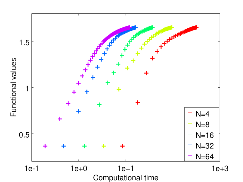
Figure 6: Same as Fig 5 but for a Newton solver.

$\displaystyle N$	$\displaystyle N\cdot t(\varepsilon,N)$
1	-
2	-
4	1264.763737
8	759.976361
16	589.424517
32	516.603943
64	774.557304

Table 3: Equivalent sequential time of ISM in the case of a Newton solver for the control of molecular orientation.

IV.3 Optimal control of Bose-Einstein condensates

The last example investigated in this work deals with the optimal control of Bose-Einstein condensates Folman et al. (2002). This subject has been extensively studied in the past few years Hohenester et al. (2007); Borzi and Hohenester (2008); Bücker et al. (2013); Jäger et al. (2014); Mennemann et al. (2015); Lapert et al. (2012c); Schaff et al. (2013). Following Ref. Hohenester et al. (2007), we consider the control of a condensate in magnetic microtraps whose dynamics is ruled by the Gross-Pitaevskii equation:

$$\frac{\partial}{\partial t}|\psi(x,t)\rangle=\left(H_{0}+V(x,\lambda(t))\right)|\psi(x,t)\rangle,$$ (11)

where $\displaystyle|\psi(x,t)\rangle$ is the state of the system, $\displaystyle H_{0}=-\frac{1}{2}\frac{\partial^{2}}{\partial{x^{2}}}+\kappa\langle\psi(x,t)|\psi(x,t)\rangle$, $\displaystyle\lambda$ is the radio-frequency control field and $\displaystyle\kappa$ a positive coupling constant. The potential $\displaystyle V$ is defined by

$$V(x,\lambda)=\left\{\begin{array}[]{cl}\frac{1}{2}\left(|x|-\frac{\lambda d}{2}\right)^{2}&{\rm for}\ |x|>\frac{\lambda d}{4}\\ \frac{1}{2}\left(\frac{(\lambda d)^{2}}{8}-x^{2}\right)&{\rm otherwise,}\end{array}\right.$$

with $\displaystyle d>0$. Unitless parameters are used here. We refer the reader to Ref. Hohenester et al. (2007) for details on the model system. The figure of merit associated with this control problem is:

$${\cal J}[\lambda]=\Re[\langle\psi(T)|\psi_{f}\rangle].$$ (12)

The final and initial states of the control problem are respectively the ground states of the Hamiltonians $\displaystyle H_{0}+V(x,0)$ and $\displaystyle H_{0}+V(x,1)$. The parameter $\displaystyle\alpha$ is set to 0.

Due to the nonlinearity of the model system, the preceding approach has to be adapted. In this way, we do not consider anymore the sequence of states $\displaystyle|\varphi_{n}^{u}\rangle$ [see Eq. (4)] but we split up these intermediate states into two sets. The sequence of initial states is taken on the trajectory $\displaystyle|\psi(t)\rangle$, i.e. defined by $\displaystyle|\psi(t_{n})\rangle$, $\displaystyle n=0,\cdots,N$, while the sequence of target states is taken on the adjoint trajectory $\displaystyle|\chi(t)\rangle$, i.e. defined by $\displaystyle|\chi(t_{n})\rangle$, $\displaystyle n=0,\cdots,N$. The maximization problem in Step 2c of Algorithm 1 is therefore replaced by the maximization of the sub-functional:

$$\mathcal{J}_{n}[u_{n},|\psi^{u}\rangle]=\Re[\langle\psi_{n}(t_{n+1})|\chi(t_{n+1})\rangle],$$ (13)

with $\displaystyle 0\leq n\leq N-1$. In this problem, the state $\displaystyle|\psi_{n}\rangle$ is defined on $\displaystyle[t_{n},t_{n+1}]$ by Eq. (5), but starting from $\displaystyle|\psi_{n}(t=t_{n})\rangle=|\psi(t_{n})\rangle$. The rest of the procedure remains unchanged.

Figure 7: Evolution of the normalized figure of merit at each iteration and for various values of $\displaystyle N$ with respect to computational time for the control of a Bose-Einstein condensate.

This modification does not affect dramatically the computational time since these trajectories are not computed sequentially but in parallel. We then use the propagator assembling technique presented in Sec. IV to compute the sequences of initial and final states. The numerical values of the parameters are set to $\displaystyle T=8$, $\displaystyle\kappa=1$ and $\displaystyle d=10$. The space domain we consider is $\displaystyle[-10,10]$. For the space discretization, we consider a uniform grid composed of $\displaystyle 50$ points. The time discretization is achieved with a time grid of $\displaystyle 2^{9}$ points, and we use Strang’s splitting (8) to compute the trajectories. The optimization solver in Step 2c consists in one iteration of the constant step gradient descent method, see Eq. (9), with $\displaystyle\rho=10^{-1}$.

The results are presented in Fig. 7.

$\displaystyle N$	$\displaystyle Eff^{\star}(\varepsilon,N)$
1	100%
2	90%
4	99.7%
8	126.3%
16	141.8%
32	116.65%

Table 4: Efficiency of ISM for various values of $\displaystyle N$ in the case of the control of a Bose-Einstein condensate.

We observe that the full efficiency is reached, as confirmed in Table 4. This feature is certainly a consequence of the nonlinear setting. The sub-control problems are simpler not only because of the size reduction induced by the time decomposition, but also because of the dynamics itself, which is simplified on a shorter time interval.

V Conclusion and perspectives

In this work, we have investigated the numerical efficiency of a time parallelized optimal control algorithm on standard quantum control problems extending from the manipulation of spin systems and molecular orientation to the control of Bose-Einstein condensates. We have shown that the full efficiency can be reached in the case of a linear dynamics optimized by means of gradient methods. On the contrary, full efficiency is not achieved when using monotonic algorithms and Newton solvers. In the case of a Newton method, the parallelization setting reduces the length of time intervals where the solver is used, and makes the subproblems easier to solve. Such a property is also observed in the case of nonlinear dynamics, as shown with the example of Bose-Einstein condensates. The results of this work can be viewed as an important step forward for the implementation of parallelization methods in quantum optimal control algorithms. Their use will become a prerequisite in a near future to simulate quantum systems of increasing complexity.

ACKNOWLEDGMENT
S.J. Glaser acknowledges support from the DFG (Gl 203/7-1), SFB 631 and the BMBF FKZ 01EZ114 project. D. Sugny and S. J. Glaser acknowledge support from the ANR-DFG research program Explosys (ANR-14-CE35-0013-01; DFG-Gl 203/9-1). J.S was partially supported by the Agence Nationale de la Recherche (ANR), Projet Blanc EMAQS number ANR-2011-BS01-017-01. This work has been done with the support of the Technische Universität München – Institute for Advanced Study, funded by the German Excellence Initiative and the European Union Seventh Framework Programme under grant agreement 291763.

References

- D’Alessandro (2008) D. D’Alessandro, Introduction to Quantum Control and Dynamics (Chapman and Hall, Boca Raton, 2008), applied mathematics and nonlinear science series ed.
- Brumer and Shapiro (2003) P. Brumer and M. Shapiro, Principles and Applications of the Quantum Control of Molecular Processes (Wiley Interscience, 2003).
- Brif et al. (2010) C. Brif, R. Chakrabarti, and H. Rabitz, New J. Phys. 12, 075008 (2010).
- Glaser et al. (2015) S. J. Glaser, U. Boscain, T. Calarco, C. P. Koch, W. Kockenberger, R. Kosloff, I. Kuprov, B. Luy, S. Schirmer, T. Schulte-Herbrüggen, et al., Eur. Phys. J. D 69, 79 (2015).
- Altafini and Ticozzi (2012) C. Altafini and F. Ticozzi, IEEE Trans. Automat. Control 57, 1898 (2012).
- Dong and Petersen (2010) D. Dong and I. A. Petersen, IET Control Theory A. 4, 2651 (2010).
- Khaneja et al. (2005) N. Khaneja, T. Reiss, C. Kehlet, T. Schulte-Herbrüggen, and S. J. Glaser, J. Magn. Reson. 172, 296 (2005).
- Reich et al. (2012) D. Reich, M. Ndong, and C. P. Koch, J. Chem. Phys. 136, 104103 (2012).
- Doria et al. (2011) P. Doria, T. Calarco, and S. Montangero, Phys. Rev. Lett. 106, 190501 (2011).
- Levitt (2008) M. H. Levitt, Spin Dynamics: Basics of Nuclear Magnetic Resonance (Wiley, New York, 2008).
- Ernst et al. (1987) R. R. Ernst, G. Bodenhausen, and A. Wokaun, Principles of nuclear magnetic resonance in one and two dimensions, vol. 14 (Clarendon Press Oxford, 1987).
- Assémat et al. (2010) E. Assémat, M. Lapert, Y. Zhang, M. Braun, S. J. Glaser, and D. Sugny, Phys. Rev. A 82, 013415 (2010).
- Lapert et al. (2012a) M. Lapert, J. Salomon, and D. Sugny, Phys. Rev. A 85, 033406 (2012a).
- Lapert et al. (2010) M. Lapert, Y. Zhang, M. Braun, S. J. Glaser, and D. Sugny, Phys. Rev. Lett. 104, 083001 (2010).
- Khaneja et al. (2001) N. Khaneja, R. Brockett, and S. J. Glaser, Phys. Rev. A 63, 032308 (2001).
- Zhang et al. (2011) Y. Zhang, M. Lapert, D. Sugny, M. Braun, and S. J. Glaser, J. Chem. Phys. 134, 054103 (2011).
- Conolly et al. (1986) S. Conolly, D. Nishimura, and A. Macovski, IEEE Trans. Med. Imaging MI-5, 106 (1986).
- Bernstein et al. (2004) M. A. Bernstein, K. F. King, and Zhou, Handbook of MRI Pulse Sequences (Elsevier, Burlington-San Diego-London, 2004).
- Lapert et al. (2012b) M. Lapert, Y. Zhang, M. Janich, S. J. Glaser, and D. Sugny, Scientific Reports 2, 589 (2012b).
- Garon et al. (2013) A. Garon, S. J. Glaser, and D. Sugny, Phys. Rev. A 88, 043422 (2013).
- Boozer (2012) A. D. Boozer, Phys. Rev. A 85, 013409 (2012).
- Toselli and Widlund (2005) A. Toselli and O. B. Widlund, Domain decomposition methods - Algorithms and theory, vol. 34 (Springer Series in Computational Mathematics, 2005).
- Horton (1992) G. Horton, Commun. Appl. Num. Methods 8, 585 (1992).
- Maday et al. (2007) Y. Maday, J. Salomon, and G. Turinici, SIAM J. Num. Anal. 45, 2468 (2007).
- Gradl et al. (2006) T. Gradl, A. K. Spörl, T. Huckle, S. J. Glaser, and T. Schulte-Herbrüggen, Proc. EUROPAR 2006, Parallel Processing Lecture Notes in Computer Science 4128, 751 (2006).
- Auckenthaler et al. (2010) T. Auckenthaler, M. Bader, T. Huckle, A. Spörl, and K. Waldherr, Parallel computing archive 36, 359 (2010).
- Palao and Kosloff (2003) J. P. Palao and R. Kosloff, Phys. Rev. A 68, 062308 (2003).
- Salomon and Turinici (2006) J. Salomon and G. Turinici, J. Chem. Phys. 124, 074102 (2006).
- Marx et al. (2000) R. Marx, A. F. Fahmy, J. M. Myers, W. Bermel, and S. J. Glaser, Phys. Rev. A 62, 012310 (2000).
- Marx et al. (2015) R. Marx, N. Pomplum, W. Bermel, H. Zeiger, F. Engelke, A. F. Fahmy, and S. J. Glaser, Magn. Reson. Chem. 53, 442 (2015).
- Kepner and Ahalt (2004a) J. Kepner and S. Ahalt, Journal of Parallel and Distributed Computing 64, 997 (2004a).
- Kepner and Ahalt (2004b) J. Kepner and S. Ahalt, Journal of Parallel and Distributed Computing 64, 997 (2004b).
- Stapelfeldt and Seideman (2003) H. Stapelfeldt and T. Seideman, Rev. Mod. Phys. 75, 543 (2003).
- Seideman and Hamilton (2006) T. Seideman and E. Hamilton, Adv. At. Mol. Opt. Phys. 52, 289 (2006).
- Znakovskaya et al. (2009) S. Znakovskaya, D. Ray, F. Anis, N. G. Johnson, I. A. Bocharova, M. Magrakvelidze, B. D. Esry, C. L. Cocke, I. V. Litvinyuk, and M. F. King, Phys. Rev. Lett. 103, 153002 (2009).
- Fleischer et al. (2011) S. Fleischer, Y. Zhou, R. W. Field, and K. A. Nelson, Phys. Rev. Lett. 107, 163603 (2011).
- Dion et al. (2001) C. M. Dion, A. Keller, and O. Atabek, Eur. Phys. J. D 14, 249 (2001).
- Averbukh and Arvieu (2001) I. S. Averbukh and R. Arvieu, Phys. Rev. Lett. 87, 163601 (2001).
- Daems et al. (2005) D. Daems, S. Guérin, D. Sugny, and H. R. Jauslin, Phys. Rev. Lett. 94, 153003 (2005).
- Lapert and Sugny (2012) M. Lapert and D. Sugny, Phys. Rev. A 85, 063418 (2012).
- Tehini and Sugny (2008) R. Tehini and D. Sugny, Phys. Rev. A 77, 223407 (2008).
- Salomon et al. (2005) J. Salomon, C. M. Dion, and G. Turinici, J. Chem. Phys. 123, 144310 (2005).
- Lapert et al. (2008) M. Lapert, R. Tehini, G. Turinici, and D. Sugny, Phys. Rev. A 78, 023408 (2008).
- Yoshida and Ohtsuki (2014) M. Yoshida and Y. Ohtsuki, Phys. Rev. A 90, 013415 (2014).
- Nakajima et al. (2012) K. Nakajima, H. Abe, and Y. Ohtsuki, J. Phys. Chem. A 116, 11219 (2012).
- Sugny et al. (2005) D. Sugny, A. Keller, O. Atabek, D. Daems, C. M. Dion, S. Guérin, and H. R. Jauslin, Phys. Rev. A 71, 063402 (2005).
- Salomon (2007) J. Salomon, ESAIM: M2AN 41, 77 (2007).
- Barret et al. (1994) R. Barret, M. Berry, T. F. Chan, J. Demmel, J. M. Donato, J. Dongarra, V. Eijkhout, R. Pozo, J. CharlKepner, and S. Ahalt, Templates for the Solution of Linear Systems: Building Blocks for Iterative Methods (SIAM, Philadelphia, 1994).
- Saad and Schultz (1986) Y. Saad and M. H. Schultz, SIAM J. Sci. Stat. Comput. 7, 856 (1986).
- Folman et al. (2002) R. Folman, P. Krüger, J. Schmiedmyaer, J. Denschlag, and C. Henkel, Adv. At. Mol. Opt. Phys. 48, 263 (2002).
- Hohenester et al. (2007) U. Hohenester, P. K. Rekdal, A. Borzi, and J. Schmiedmayer, Phys. Rev. A 75 (2007).
- Borzi and Hohenester (2008) A. Borzi and U. Hohenester, SIAM J. Sci. Comput. 30, 441 (2008).
- Skinner and Glaser (2002) T. Skinner and S. J. Glaser, Phys. Rev. A 66, 032112 (2002).
- Bücker et al. (2013) R. Bücker, T. Berrada, S. van Frank, J.-F. Schaff, T. Schumm, J. Schmiedmayer, G. Jäger, J. Grond, and U. Hohenester, J. Phys. B 46, 104012 (2013).
- Jäger et al. (2014) G. Jäger, D. M. Reich, M. H. Goerz, C. P. Koch, and U. Hohenester, Phys. Rev. A 90, 033628 (2014).
- Mennemann et al. (2015) J. F. Mennemann, D. Matthes, R.-M. Weishäupl, and T. Langen, New J. Phys. 17, 113027 (2015).
- Lapert et al. (2012c) M. Lapert, G. Ferrini, and D. Sugny, Phys. Rev. A 85, 023611 (2012c).
- Schaff et al. (2013) J.-F. Schaff, X.-L. Song, P. Capuzzi, P. Vignolo, and G. Labeyrie, Eur. Phys. Lett. 93, 23001 (2013).