Kulfi: Robust Traffic Engineering
Using Semi-Oblivious Routing

Abstract

Wide-area network traffic engineering enables network operators to reduce congestion and improve utilization by balancing load across multiple paths. Current approaches to traffic engineering can be modeled in terms of a routing component that computes forwarding paths, and a load balancing component that maps incoming flows onto those paths dynamically, adjusting sending rates to fit current conditions. Unfortunately, existing systems rely on simple strategies for one or both of these components, which leads to poor performance or requires making frequent updates to forwarding paths, significantly increasing management complexity. This paper explores a different approach based on semi-oblivious routing, a natural extension of oblivious routing in which the system computes a diverse set of paths independent of demands, but also dynamically adapts sending rates as conditions change. Semi-oblivious routing has a number of important advantages over competing approaches including low overhead, nearly optimal performance, and built-in protection against unexpected bursts of traffic and failures. Through in-depth simulations and a deployment on SDN hardware, we show that these benefits are robust, and hold across a wide range of topologies, demands, resource budgets, and failure scenarios.

1 Introduction

Wide-area network (WAN) traffic engineering (TE) is a topic of interest for many leading technology companies including Amazon, Facebook, Google, Microsoft, Netflix, and others. The private networks operated by these companies must balance demands between latency-sensitive, customer-facing traffic and high-volume, operational traffic, such as bulk replication for large data stores. A common objective is to improve network utilization by distributing load across multiple paths to obtain better operational efficiency. Towards this goal, a variety of approaches have been explored in recent years, each relying on a different combination of underlying strategies for computing paths and distributing load [46, 43, 24, 26].

The textbook approach to traffic engineering frames it as a combinatorial optimization problem: given a capacitated network and a set of demands for flow between sources and destinations, find an assignment of flows to paths that optimizes for some criterion, such as minimizing the maximum amount of congestion on any link. This is known as the multi-commodity flow (MCF) problem in the literature, and has been extensively studied. If the flow between each source and destination is restricted to use a single path, then the problem is NP-complete. But, if fractional flows are allowed, then optimal solutions can be found in polynomial time using linear programming (LP). Scalability and running time can be further improved by relaxing the optimality requirement and using an approximation algorithm, such as the multiplicative weights method [34, 17, 6].

Optimal traffic engineering.  In principle, it is possible to build an optimal traffic engineering system by repeatedly executing the following steps in a loop: (i) monitor the network load and build up an estimate of the demands for traffic between each source-destination pair; (ii) translate the demands into an LP and use an off-the-shelf solver to compute an optimal set of forwarding paths; and (iii) update the configurations of network switches to implement those paths. However, to actually build such a system, one would have to overcome a number of major practical challenges:

• Solving MCF instances could become a bottleneck, especially at scale and in dynamic environments where solutions would need to be computed frequently to stay close to the optimum.

• Estimating demands accurately could be difficult, especially with unexpected failures and traffic bursts.

• Switches have limited amounts of memory for implementing paths, but it is not clear how to limit MCF to abide by resource budgets.

• Small changes in demands could produce dramatically different paths, which would lead to excessive churn.

• Updating configurations in a consistent manner could be difficult and would add significant complexity to the management infrastructure [40, 28].

• Switches could take several seconds to implement updates, which imposes a limit on how rapidly the system can adapt to changing conditions.

Centralized traffic engineering.  One way to side-step these challenges is to pre-compute a set of forwarding paths and distribute flows onto those paths dynamically—e.g., using the global visibility offered by a logically-centralized SDN controller. This approach gives up on optimality, since it pre-commits to using a restricted set of paths, but it retains many of the benefits of MCF-based approaches and is much simpler to implement. In particular, it only requires the ability to update sending rates at the edge of the network rather than changing end-to-end forwarding paths at each iteration. By restricting attention to relatively small topologies, scheduling traffic with elastic demands, and using heuristic approximation algorithms, systems such as B4 [26] and SWAN [24] have been able to obtain dramatic improvements in production settings. However, one important aspect of these systems has been under-explored: the algorithms they use to select forwarding paths. B4 uses a greedy heuristic that attempts to ensure fairness while SWAN uses $k$-shortest paths. Relying on simple and somewhat ad hoc path selection algorithms means that these systems sometimes lack sufficient flexibility and path diversity to handle unexpected situations such as estimation errors, traffic bursts, link failures, etc.

Our approach: Semi-oblivious traffic engineering.  This paper investigates a simple question: can we improve traffic engineering systems by selecting paths in a better way? We answer this question positively, showing that by combining oblivious routing (originally formulated by Räcke [37, 38]) with dynamic rate adaptation, it is possible to obtain a traffic engineering system that provides substantial performance improvements while remaining simple to implement and easy to manage. Moreover, these benefits continue to hold under a wide range of topologies, demands, resource budgets, and failure scenarios. We call this hybrid approach semi-oblivious traffic engineering (SOTE).

Prior work.  The idea of using oblivious routing for wide-area network traffic engineering was originally proposed in a seminal paper by Applegate and Cohen [4]. They showed that on practical workloads, oblivious routing performs much better than is predicted by the worst-case bounds, but they did not investigate whether performance could be further improved by incorporating dynamic rate adaptation. Similarly, while the combination of oblivious routing and dynamic rate adaptation has been explored in the theory literature, prior work did not develop an implementation and focused on establishing lower bounds with artificial topologies and demands [22]. This work is the first we are aware of to describe an implementation of semi-oblivious routing and a comprehensive evaluation on realistic workloads.

Implementation.  We have implemented SOTE in a new framework called Kulfi that provides a rich collection of library functions designed to support rapid development of traffic engineering algorithms, as well as simulation and hardware deployments. To date, we have implemented 13 different traffic engineering algorithms, 7 traffic prediction algorithms, and evaluated them on 9 different topologies from widely-known ISPs. The Kulfi simulator includes tunable parameters for demands, failure scenarios, path budgets, etc. to simulate a variety of realistic workloads.

Experience.  The results of our experiments and simulations are extremely promising. When oblivious routing is enhanced with a rate adaptation component the congestion ratios we measure are competitive with the best known traffic engineering solutions, and far better than the worst-case scenarios predicted in the theory literature. We attribute these results to qualities of the paths computed by oblivious routing: they are low-stretch, diverse, and naturally balance load, guaranteeing worst-case congestion that is within a logarithmic factor of optimal.

Contributions.  Our main contributions are as follows:

1. We survey various approaches to traffic engineering in wide area networks (§2).

2. We present SOTE, a new approach to traffic engineering that enriches oblivious routing with dynamic rate adaptation (§3).

3. We describe an implementation of SOTE and other traffic engineering schemes in Kulfi (§4).

4. We conduct simulations and experiments comparing SOTE against other approaches and compare performance with respect to a large number of criteria including congestion, latency, throughput, loss, resource usage, etc. (§5-7).

Outline.  The rest of this paper is organized as follows. The next section provides a short summary of various approaches to traffic engineering in wide area networks (§2). We then present a detailed description of oblivious and semi-oblivious routing (§3). We describe our implementation (§4) and present the results of experiments demonstrating that SOTE is competitive with other approaches on realistic workloads using an SDN-based hardware testbed (§5) and comprehensive simulations (§7). Finally, we discuss related work (§8) and conclude (§9).

2 Background

We briefly survey some of the main approaches to traffic engineering, both in theory and in practice, to lay the groundwork for understanding SOTE.

In practice.  The traditional approach to traffic engineering, which has been used for many years, is to carefully tune link weights in distributed routing protocols, such as OSPF, so they compute a near-optimal set of forwarding paths [16, 15]. This approach is simple to implement, as it harnesses the capabilities of widely-deployed traditional protocols, but it requires having accurate estimates of traffic demands. Moreover, it often leads to poor performance when failures occur or during periods of re-convergence after link weights are modified to reflect new demands.

Another common strategy is to use equal-cost multi-path routing (ECMP). Each switch computes a hash over packet headers, and routes along a randomly selected least-cost path to the destination. Because forwarding decisions are made without global knowledge, ECMP is simple to implement, but these local decisions sometimes lead to extra congestion [32]. In addition, the performance of ECMP is fundamentally restricted by its use of least-cost paths, and often performs poorly in the presence of “elephant” flows [2, 3].

Several recent systems have exploited the global visibility offered by SDN controllers to distribute traffic across pre-computed paths in near-optimal ways. SWAN [24] distributes flow across $k$-shortest paths, using a variant of the standard LP formulation that reserves a small amount of “scratch capacity” for configuration updates. The system proposed by Suchara et al. [43] incorporates failures into the LP formulation and computes a diverse set of paths offline. It then uses a simple local strategy to dynamically adapt sending rates at each source. B4 [26] distributes flow across multiple paths to improve utilization while ensuring fairness, and uses a heuristic approximation to improve scalability.

In theory.  There is also a significant body of traffic engineering work in the theory community. One line of work has focused on improving running times for MCF by relaxing the optimality requirement, and instead using approximation algorithms, such as the multiplicative weights method [6, 17, 34]. For example, Awerbuch and Khandekar [7] adapted the multiplicative weights method for distributed settings, improving the scalability of the approach. However, like all MCF-based schemes, this approach suffers from sensitivity to estimation accuracy, difficulties related to fault tolerance, excessive path churn, and high management complexity [4].

To overcome these challenges, another line of work has explored the space of algorithms that provide strong guarantees in the presence of arbitrary demands. For example, Valiant load balancing (VLB) routes traffic in a complete mesh via randomly selected intermediate nodes. Originally proposed as a way to load balance message routing on parallel computers [44], VLB has recently been applied in a number of other settings including datacenter networks, wide-area networks, and software switches [5, 13, 19, 46]. However, on the negative side, sending traffic through intermediate nodes increases path length, which can increase latency dramatically—e.g., consider routing traffic from New York to Seattle through Europe. Furthermore, VLB can exhibit degraded performance compared to the optimum when traffic is dropped due to congestion [12].

Oblivious routing generalizes VLB from meshes to arbitrary topologies. It computes a probability distribution on low-stretch paths in advance and forwards traffic according to that distribution no matter what demands occur when deployed—in other words, it is oblivious to the actual demands. Remarkably, there exist oblivious routing schemes whose congestion ratio is never worse than $O(\log{n})$ factor of optimal. The simplest scheme, first proposed in a breakthrough paper by Räcke [38], constructs a set of tree-structured overlays and then uses these overlays to construct random forwarding paths between all source-destination pairs.

While the $O(\log{n})$ congestion ratio for oblivious routing is surprisingly strong for a worst-case guarantee, it still requires that network operators over-provision capacity by a significant amount. Applegate and Cohen [4] showed that, in practice, oblivious routing performs better than the worst-case predictions, but a straightforward adoption of oblivious routing is still not competitive with systems that rebalance load dynamically. Consequently, the overall verdict seems to be that oblivious routing is an elegant mathematical result with important applications in the theory of approximation algorithms (e.g. for minimum bisection [38]), but as a traffic engineering method it is of limited practical value.

Routing Algorithm	Description	Type	Path	Max	Overheads
			Diversity	Congestion	Churn	Recovery
MCF	Multi-Commodity Flow solved with LP [20]	conscious	medium	least	high	slow
MW	Multi-Commodity Flow solved with Multiplicative Weights [17]	conscious	medium	least	high	slow
SPF	Shortest Path First	oblivious	least	high	none	none
ECMP	Equal-Cost, Multi-Path	oblivious	low	high	none	fast
KSP	K-Shortest Paths	oblivious	medium	medium	none	fast
Räcke	Räcke [38]	oblivious	high	low	none	fast
VLB	Valiant Load Balancing [44]	oblivious	high	medium	none	fast
SemiMCF-MCF	MCF for paths MCF for weights	semi-oblivious	medium	least	none	fast
SemiMCF-ECMP	ECMP for paths MCF for weights	semi-oblivious	low	medium	none	fast
SemiMCF-KSP	KSP for paths MCF for weights	semi-oblivious	medium	medium	none	fast
SemiMCF-Räcke	Räcke for paths MCF for weights	semi-oblivious	high	low	none	fast
SemiMCF-VLB	VLB for paths MCF for weights	semi-oblivious	high	medium	none	fast
SemiMCF-MCF-Env	MCF over demand envelope for paths MCF for weights [43]	semi-oblivious	medium	low	none	fast
SemiMCF-MCF-FT-Env	Multiple MCF-Env considering failures MCF for weights [43]	semi-oblivious	high	medium	none	fast

Table 1: Summary of routing algorithms implemented in Kulfi.

Discussion.  Prior work demonstrates that (i) traffic engineering algorithms that use a static set of pre-computed paths can avoid churn and reduce management overhead, but (ii) the straightforward adaptation of oblivious routing requires unacceptable over-provisioning, and (iii) although optimizing over the full set of multi-commodity flows is too heavyweight as a complete strategy, optimizing the distribution of flow over a limited set of paths (e.g. using an LP solver, or iterative methods) appears to work well in practice. As mentioned above, several systems have proposed instances of this approach, including SWAN [24], B4 [26], and the work of Suchara et al. [43].

Outlook.  In this paper, we advocate for using oblivious routing as a method for selecting routing paths, while combining it with optimization techniques (e.g., LP solvers) to continually adjust the distribution of flow across those paths. The resulting traffic engineering scheme has both strong theoretical guarantees and outperforms the state of the art in simulations of realistic scenarios.

3 Semi-oblivious Routing

We now present the key building blocks used in SOTE. We first review Räcke’s oblivious algorithm and then discuss methods for dynamically adjusting sending rates.

Räcke’s Algorithm.  At the core of Räcke’s algorithm is a structure we call a routing tree. A routing tree determines a unique forwarding path between every source-destination pair in the network: one simply concatenates the sub-paths corresponding to edges on the tree path connecting the pair. In more detail, a routing tree comprises (i) a logical tree topology $T$ whose leaves are in one-to-one correspondence with nodes of the physical topology, $G$; and (ii) a mapping that assigns to each edge of $T$ a corresponding path in $G$. Such a structure implicitly defines a routing path for every source-destination pair $(s,t)$. One can obtain a path from $s$ to $t$ by finding the corresponding leaves of $T$, identifying the edge set of the path in $T$ that joins these two leaves, and concatenating the corresponding physical paths in $G$. Figure 1 illustrates this process of using a routing tree to construct a physical path.

Figure 1: A logical representation of a routing tree, and its physical mapping.

Going a step further, one can define a randomized routing tree to be a probability distribution over routing trees. Such a structure defines a probability distribution over routing paths for every source $s$ and destination $t$, by randomly sampling one tree from the distribution and selecting the $s$-$t$ routing path defined by the sampled tree. As an illustration of the expressiveness of randomized routing trees, observe that Valiant load balancing (VLB) can be viewed as a specific instantiation of the general idea. The logical tree topology in this case consists of a root vertex directly attached to leaves corresponding to the nodes of the physical topology. To sample from the probability distribution over routing trees, one first samples a location for the root vertex at random from the nodes in the physical topology, and then identifies each tree edge with the shortest path between the corresponding physical nodes. In general, one can think of randomized routing trees as a hierarchical generalization of VLB, where the network is recursively partitioned into progressively smaller subsets, and routing from a source to a destination requires passing through a random intermediate node corresponding to the level of the hierarchy at which the source and destination are grouped into different pieces of the partition.

Räcke also proposed an efficient, iterative algorithm for constructing randomized routing trees. In each iteration, the algorithm defines a length for each edge of the physical network. Initially the length of an edge is the inverse of its capacity, and it is updated multiplicatively at the end of each iteration in a manner to be described later. For a specified set of edge lengths, the stretch of an edge $e=(u,v)$ relative to a routing tree $T$ is defined to be the ratio between the length of the path from $u$ to $v$ defined by $T$, and the length of the one-hop path defined by $e$. The average stretch of a routing tree is computed by averaging the stretch of each edge, weighted by its capacity. The key subroutine in Räcke’s algorithm is the FRT algorithm [14], which takes as input a set of edge lengths and outputs a routing tree whose average stretch is at most $O(\log n)$. Each iteration of Räcke’s algorithm invokes FRT using the current edge lengths to obtain a routing tree $T$. Then, for each edge $e$ in the physical topology it computes a “utilization” parameter $u(e,T)$ which constitutes a worst-case upper bound on the congestion that may be induced on $e$ using $T$ as a routing tree. The routing tree $T$ is then added as a support point to the distribution, with a probability inversely proportional to $u_{\max}=\max_{e}\{u(e,T)\}$. Finally, to update the length of each edge $e$, we multiply by $(1+\epsilon)^{u(e,T)/u_{\max}}$, for some constant $\epsilon>0$. In our implementation we use $\epsilon=0.1$. This loop iterates until there exists an edge $e$ whose combined utilization $\sum_{T}u(e,T)$ (summing over the trees selected in all previous iterations of the loop) exceeds a predetermined threshold.

It is worth pointing out some of the features of the set of paths selected by Räcke’s oblivious routing algorithm. First, since each routing tree is a low-stretch tree arising from one application of the FRT algorithm, Räcke’s oblivious routing is biased toward low-stretch paths. This contrasts with VLB, which tends to choose circuitous paths, especially when the source and destination are near one another. Second, since FRT is a randomized algorithm, the repeated application of FRT in Räcke’s algorithm tends to result in a diverse set of paths for most source-destination pairs. This path diversity is beneficial for routing around edge or node failures without having to recompute the entire routing scheme. Third, in any iteration of the algorithm, the length of an edge is an exponentially-increasing function of its utilization in previous iterations. The inclusion of long edges in routing paths is costly from the standpoint of constructing a routing tree with low average stretch. Thus, the routing paths selected in any iteration of Räcke’s algorithm tend to avoid reusing edges that have been heavily utilized in prior iterations. This leads to good load-balancing properties, e.g. the $O(\log n)$ congestion ratio guarantee described in Section 2.

Semi-oblivious routing.  Oblivious routing schemes do not adjust the relative distribution of flow across paths between a given source and destination. This limitation means they cannot fine-tune the distribution of flow to continually re-optimize it as demands evolve. It leads to inefficient utilization of network capacity and requires overprovisioning to avoid congestion. Applegate and Cohen [4] investigated the performance of oblivious routing in practice and found that, in contrast the $O(\log n)$ overprovisioning suggested by Räcke’s worst-case result, in most cases it is sufficient to overprovision the capacity of each edge by a factor of 2 or less. But while this is better than the worst-case bounds, it is still not competitive with state-of-the-art methods.

These observations suggest an investigation of routing schemes that use a static set of paths (as in oblivious routing) but dynamically adjust the distribution of flow over those paths as the traffic matrix varies and/or the network suffers edge or node failures. The combination of a static set of paths and time-varying probability distributions over those paths has been called semi-oblivious routing [22]. Unfortunately, from a worst-case standpoint, semi-oblivious routing is not significantly better than fully oblivious routing. Hajiaghayi et al. [22] proved that any semi-oblivious routing scheme that uses polynomially many forwarding paths must suffer a congestion ratio of $\widetilde{\Omega}(\log{n})$ in the worst case, even when the network is as simple as a planar grid. (The actual lower bound of [22] is $\log{(n)}/\log{(\log{(n)})}$, leaving open the possibility of a very small asymptotic improvement). On the other hand, the traffic matrices involved in this lower bound construction are highly unnatural, leaving open the possibility that under realistic workloads, semi-oblivious routing may significantly outperform oblivious routing, and may even approach or match the performance of optimal MCF.

Implementing semi-oblivious routing requires defining two algorithms: one executed at set-up time to select the static set of forwarding paths, and another executed repeatedly at run-time to choose how to distribute flow over those paths. Table 1 lists the algorithms we have implemented in Kulfi including five path selection algorithms. Three of these (SPF, KSP, ECMP) select shortest paths or near-shortest-paths, another (VLB) selects paths by concatenating the shortest paths to a random intermediary node and then to the destination, and the oblivious scheme (Räcke) just described. For distributing flow over paths, in addition to oblivious schemes (which choose a distribution at initialization time and do not re-compute at runtime) we have implemented three algorithms for dynamically adjusting distributions. Semi-MCF uses an LP solver to minimize the maximum edge congestion when all flow is routed over the allowed set of paths. Semi-with-MCF-Envelope also uses an LP solver, but solves a different optimization problem that minimizes a worst-case upper bound on the congestion under all possible scenarios [43].

4 Kulfi Toolkit

$\begin{array}[]{r@{\;}c@{\;}l@{\quad}r@{\;}c@{\;}l@{\quad}r@{\;}c@{\;}l}T&=&\textit{Topologies}&P&=&\textit{Paths}&H&=&\textit{Hosts}\\ \end{array}$
$\begin{array}[]{r@{\;}c@{\;}l@{\quad}l}\hline\cr D&\in&(H\times H)\rightarrow\mathbb{R}&\text{Demand}\\ S&\in&(H\times H)\rightarrow P\rightarrow\mathbb{R}&\text{Scheme}\\ A&\in&(T\times D\times S)\rightarrow S&\text{Algorithm}\\ \hline\cr\end{array}$

Figure 2: Domains and Types for Kulfi Modules

To facilitate making quantitative comparisons between different traffic engineering approaches, we developed a software toolkit called Kulfi. Kulfi provides a set of basic primitives and extensible mechanisms for rapidly developing and experimenting with a wide variety of traffic engineering algorithms, both in simulation and using SDN hardware.

4.1 Algorithm Modules

We assume that any traffic engineering algorithm will have access the network topology (which distinguishes between hosts and forwarding devices), and a list of demand matrices, where a single such matrix is a mapping from a source-destination pair to requests for bandwidth. The demands may be measured or predicted.

A routing scheme is a mapping from source-destination pairs to distributions on paths between those nodes. For example, a shortest path routing scheme, given an input $(u,v)$ would return a single path (i.e., the shortest path from $u$ to $v$) with probability $1.0$. As we will see, other schemes may return a set of paths, each weighted by a different probability.

A routing algorithm produces a routing scheme. In the simplest case, the routing algorithm can compute a scheme using only the topology and demands. However, some routing algorithms must be initialized with an existing scheme to produce a modified scheme. Thus, in general, a routing algorithm takes a topology, a set of demands, and a (possibly empty) scheme as input, and produces a scheme as output. A routing algorithm may be invoked repeatedly, in response to changes in input (e.g., changes in demands or the topology).

Kulfi allows users to run different traffic engineering algorithms by implementing modules that conform to the interfaces in Table 2. These interfaces match the definitions above. From these definitions, we see there are two axes along which routing algorithms may differ: how they select paths and how they assign probabilities to those paths. These two axes lead to three natural classifications for routing algorithms. An oblivious routing algorithm is one that uses a fixed set of paths and probabilities, and does not alter those choices in subsequent invocations. A semi-oblivious approach is algorithm uses a fixed set of paths, but alters the probabilities of those paths with each invocation. To the best of our knowledge, there is no standardized term for algorithms that alter the paths and probabilities at each invocation, so we call these algorithms conscious. The fourth alternative (i.e., an algorithm that changes paths without changing probabilities) would not be possible.

We have implemented 13 different algorithms in Kulfi, summarized in Table 1. Among these algorithms, SWAN corresponds to the Semi-Oblivious with MCF initialized with K-Shortest Paths. Suchara et al. [43] corresponds to Semi-Oblivious with MCF initialized with solving MCF (using an envelope of demands) over all possible failure scenarios. We simulate the inclusion of failures by repeatedly re-solving on different input topologies. Note that these two approaches are functionally equivalent for metrics related to fault tolerance. They differ for metrics related to solving time. But, as we do we do not include the time spent re-solving as part of the running time in our simulation, the measurements are slightly better than expected for a direct implementation.

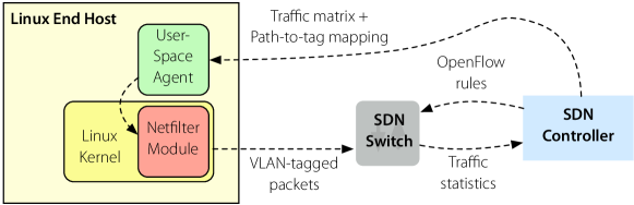
Figure 3: Implementation architecture.

4.2 System Infrastructure

Kulfi modules can be executed within a simulator, as we will discuss in Section 7, or deployed on actual networks using a combination of software-defined networking and source-based routing. This design is inspired by Pathlet routing [18] or Casado’s fabric [11]. In our source-routing scheme, each edge in the network is assigned a unique identifier. A path enumerates the edges from a source to a destination in a stack of identifiers. To route, each switch along the path simply “pops” the top of the stack, and forwards out the appropriate port. It is important to note that none of the algorithms described in this paper require SDN or source-routing. However, this approach allowed us to easily implement and compare many different approaches schemes.

Figure 3 shows the basic architecture for our implementation. There are four major components, which we will describe in detail below: (i) an SDN controller, (ii) an OpenFlow-enabled switch, (iii) an end-host agent in user space, and (iv) an end-host kernel module.

SDN controller.  The SDN controller performs four functions. First, it computes the forwarding paths for the particular traffic engineering scheme (e.g., shortest path, optimal MCF, or Räcke’s algorithm). It then maps the computed paths to their corresponding stack of identifiers in the physical network. Second, it installs the appropriate forwarding rules in the SDN switch. Third, it sends the path-to-identifier mappings to each of the user-space end-host agents in the network. Finally, it periodically gathers traffic statistics from the SDN switches, computes the demands, and sends estimated demands to the user-space agents on end hosts.

OpenFlow-enabled switch.  The switches route traffic by examining the identifier stack in the packet, popping the top of the stack to get the next identifier in the path, and outputting the packet on the port indicated by the identifier. Our prototype used VLAN tags to store the stack of identifiers, although we could have also used MPLS labels. The switches also maintain counters that collect statistics about the amount of traffic sent across each link.

End-host user-space agent.  The end-host user-space agent serves as an intermediary between the SDN controller and the end-host kernel module. The agent listens on a designated port for messages from the controller, which contain the path-to-identifier mappings and a periodically updated global traffic matrix. The agent communicates this information to the kernel module through the /proc file system.

End-host kernel module.  The main responsibility of the kernel module is to assign the appropriate path to each packet. Packets from the same flow are always sent along the same paths. Thus, each time the module processes an outgoing packet, it checks if the packet is part of an existing flow. If it is not, it assigns the flow a path, and maintains that information in a hash table. If it is part of a flow, then it retrieves the path from the table. Flows are evicted from the hash table based on an idle timeout. For randomized routing schemes, the kernel module assigns the path using a weighted probability distribution.

5 Hardware Experiments

To calibrate the simulations in Section 7, we first conducted experiments on a hardware testbed using the SDN-based implementation described in Section 4.2. These experiments measured the congestion ratio for SPF, ECMP, MCF, Räcke, and the semi-oblivious variant of Räcke using different workloads on an emulated Abilene backbone [1].

Hardware testbed.  Our testbed emulates the Abilene topology (Figure 5), which consists of $12$ routers connected by $15$ links, using $3$ Pica8 Pronto 3290 physical switches and $24$ Dell R620 PowerEdge servers. Each server has two $8$-core $2.6$GHz Intel Xeon processors, $64$GB RAM, and four $1$Gb NICs. Each switch was configured with $4$ Open vSwitch instances, yielding a total of $12$ logical switches. We scaled down the historical Abilene demands to match the $1$Gbps links in our testbed.

Traffic demands.  We generated traffic using the gravity model [41] and also added artificial bursts over bottleneck links. We used our kernel module to tag outgoing packets with identifiers corresponding to the path assigned by the routing scheme. As we replayed traffic in a compressed time-scale, we configured our kernel module to treat each packet as a separate flow. These simplifications, which made it easy to conduct careful measurements, are idealizations, but we believe they are reasonable in wide-area networks where there are very large number of flows.

Experimental results.  Figures 4(a)-4(b) depict the maximum and median congestion over all links under different traffic generators. The first graph (Figure 4(a)) uses a traffic pattern in which only switches $4$ (Denver) and $7$ (Kansas City) sent traffic to switch $10$ (Sunnyvale). This experiment was crafted so that both flows share a common bottleneck link ($s4$-$s10$) and the maximum congestion for SPF and ECMP remains $1$ while the other schemes do not saturate any of the links. Next, we generated traffic based on the gravity model of estimating traffic matrices in Abilene network. Figure 4(b) shows the corresponding maximum and median link utilizations. Note that since the traffic matrices were estimated based on what could be routed through Abilene network using OSPF, these matrices tend to produce network traffic that would be feasible under SPF and ECMP. However, we still observe that the maximum congestion in the case of semi-oblivious and MCF routing schemes stay well below those for SPF and ECMP. For the final graph (Figure 4(c)), we added the artificial demand on top of the demand estimated by Gravity model and replayed it on our testbed. Again, this extra demand was not suited for shortest-paths and the maximum link congestion for SPF and ECMP shot up while remaining nearly constant for other schemes.

Overall, these experiments show that the semi-oblivious variant of Räcke is competitive with optimal MCF approaches in terms of congestion. Moreover, these results are consistent with the results that we see in our simulated environment, as we will discuss Section 7.

(a) Artificial traffic from switches $4$ and $7$ to $10$.

(b) Gravity model demands.

(c) Gravity model demands and Artificial traffic.

Figure 4: Link congestion on emulated Abilene network.

6 Experimental Setup

Traffic engineering algorithms are impacted by a number of parameters, including topology, variance in demands, prediction accuracy, and the failure model. To provide a comprehensive evaluation, we implemented a network simulator that allows us to systematically alter the possible inputs and measure the results.

Simulator.  The Kulfi simulator is a discrete event simulator that models the state of a network in response to a sequence of traffic demands. It has four required input parameters: (i) a file describing the network topology, (ii) a file containing a list of the actual traffic matrices, (iii) a file containing a list of the predicted traffic matrices, and (iv) a list of algorithms to execute. Additionally, there are a number of optional parameters including, among others, flags to vary the budget (i.e., number of paths used between a source-destination pair), a scaling factor for demands, the number of links to fail, the recovery method, and the generation of flash demands.

For each algorithm, the simulator iterates over the sequence of predicted traffic matrices, which represent the predicted demands for network sources at discrete time intervals. For each matrix, the simulator computes the routing scheme and then simulates the flow of traffic for 1,000 time steps. Every link in the network is associated with a queue. At each time step, every source adds traffic to the queue of the first link of paths it is using. Likewise, every link forwards traffic to next hop for every flow that it is handling, by placing traffic on the queue for the next link. Because links have limited capacity, as specified by the input topology file, the simulator uses max-min fair sharing to allocate bandwidth to each flow on a link. Any traffic that exceeds the link capacity is dropped. We refer to traffic dropped due to capacity constraints as congestion loss. During execution, the simulator may fail some links according to the failure model. If the simulator cannot forward traffic along a link due to failure, then that traffic is dropped. We refer to the amount of traffic that is dropped due to link failure as failure loss.

Topologies.  To ensure that our results are not limited to specific topologies, we ran simulations on all 262 topologies in the Internet Topology Zoo dataset [25]. However, to make the presentation of information accessible, we focus results on a subset of 9 topologies. We chose the 9 topologies because they are topologies that represent real-world ISPs, and they overlap with topologies used to evaluate other traffic engineering approaches in the literature [29]. To compute aggregate results, we measured the normalized throughput (and loss due to congestion or failure) as a fraction of total demand for each topology and compute averages.

Demands.  We generated demand matrices using the gravity model [41], which ascribes to each host $i$ a non-negative weight, $w_{i}$, and posits that the amount of traffic flowing from $i$ to $j$ is proportional to the product $w_{i}\cdot w_{j}$ for all pairs $i,j$. The weights $w_{i}$ in our simulations are randomly sampled from a heavy-tailed Pareto distribution obtained by fitting the observed Abilene traffic matrices. To simulate diurnal and weekly variations in traffic intensity, we rescale the total flow in each time step based on the weekly traffic patterns observed in NetFlow traces from Abilene. The patterns are modeled by randomly perturbing the Fourier coefficients of the observed time-series of total flow measurements.

To model demand variation over time, we use the Metropolis-Hastings (M-H) algorithm to sample from a Markov chain on the space of traffic matrices, whose stationary distribution is the gravity model with Pareto-distributed weights described above. The M-H algorithm updates the weight of each host from one time step to the next by randomly sampling an adjusted value for $w$ using a “proposal” distribution. In our simulations we defined the following proposal distribution for the additive adjustment, $\Delta w$, that incorporates gradual variation over time accompanied by rare discrete jumps: with probability 99%, it is $\mathcal{N}(0,w^{2}/4)$, and with probability 1%, it is uniform$([-w,-0.8w]$ $\cup$ $[0.8w,w])$.

To model flash bursts we induced sudden spikes in demand to a single sink node in the network followed by a heavy-tailed decrease back to the stationary distribution. The decreasing tail has a half-life of 30 minutes. In the experiments we pick the sink node randomly in each traffic matrix (TM). The burst amount is specified by a parameter, $\beta$. Using $d(\cdot,\cdot)$ to denote entries of the pre-flash TM, then the peak burst traffic from any host ($h$) to the sink ($s$) is given by $\beta\cdot\frac{\sum_{i}\sum_{j}d(i,j)}{n}\cdot\frac{d(h,s)}{\sum_{i}d(i,s)}$.

We scale the generated traffic matrices to make them comparable across different topologies. To do this, we multiply all of the TM’s in the randomly generated sequence by a common scalar, chosen so that the maximum congestion of an optimal MCF in the first time step is normalized to 0.4. This choice of the normalization constant is prompted by recent studies on SWAN [24] which shows that the average congestion of the maximum utilized links is around 40% to 60% in general. However, we also study the routing behavior under different scales ($S$) for demand. When scaling by $S$, we multiply all the elements in the traffic matrices such that the expected congestion for the first traffic matrix is $0.4\times S$.

Budget.  In practice, network devices are often constrained in that they can only support a limited number of forwarding rules. To evaluate how different routing algorithms are impacted by such resource constraints, we limited the number of paths that an algorithm can use between a source-destination pair. We used a budget range from one to five, as well as unconstrained. For a budget of $k$, we selected the $k$ paths with highest probabilities and re-normalized their weights. We refer to the union of the $k$-path sets for all source-destination pairs as the base path set.

Failure Model.  To evaluate how failures impact various traffic engineering algorithms, we used several failure scenarios. To create different scenarios, we varied a parameter $\phi$, ranging from $0$ to $3$, which specifies the number of failed links. The way in which failed links were chosen depends on the value of $\phi$. For $\phi>1$, we simply fail $\phi$ random links as long as it doesn’t partition the network. On the other hand, if $\phi=1$, we choose a deterministic sequence of single-link failures, to facilitate comparisons across different routing schemes. The deterministic sequence of failures is specified as follows: we sort the links based on their utilization in SPF and pick links from an evenly-spaced sequence of positions in the sorted order. In other words, if there are 24 links and 24 TMs, we would end up failing each link. If there are 24 links and 12 TMs, we fail alternate links in sorted SPF order.

Failure Recovery.  We implemented two forms of failure recovery. With global recovery, a centralized controller recomputes the routing scheme based on global knowledge of the network state, and updates forwarding rules appropriately. With local recovery, edge devices (e.g., end hosts, virtual switches in the hypervisors, or first-hop switches) respond to failures without global coordination. To implement local recovery, we remove the paths that contain the failed links from the pair’s base path set. Then we update the probabilities for the remaining paths. For SemiMCF-based schemes, these probabilities are recomputed using MCF, while for other schemes, we renormalize the probabilities to sum to 1. To implement global recovery, we remove the failed links from the input topology, and re-compute the scheme. As a baseline, we also implemented an idealized “OptimalMCF” algorithm that runs MCF every time there is a failure to compute the best scheme (in terms of congestion) based on real time demands with no prediction error. For flash crowds, it periodically runs MCF on the current demands.

Prediction.  We implemented a suite of algorithms for predicting the next traffic matrix in a sequence of TMs. These include standard machine learning methods—linear regression, lasso/ridge regression, logistic regression, random forest prediction—as well as algebraic methods (FFT fit and polynomial fit) based on approximating the time series with a Fourier-sparse or low-degree-polynomial approximation, respectively. For each pair of hosts, we perform independent time series prediction. At each time step, every algorithm predicts the demand of the current time step using the observed demands from the previous $k$ time steps; the size of the sliding window ($k$) is optimized separately for each prediction algorithm using cross-validation. The machine learning algorithms (regression algorithms and random forest) are trained using the previous $k$ time steps as $k$ features. The FFT fit and polynomial fit algorithms find a function with a bounded number of non-zero Fourier coefficients (FFT fit) or a bounded-degree polynomial function (polynomial fit) that minimizes the absolute difference between the predicted demand and the actual demand over the past $k$ time steps. This best-fit function is then evaluated in the current time step to yield the predicted demand. Polynomial fit and random forest are unstable, especially when spikes exist. Regression algorithms with regularizers, such as lasso and ridge, are more stable. But the prediction errors are usually less than 20% of the actual demand, both on real Abilene data and on the synthetic demand matrices that we generated.

Prediction Error.  We tested the sensitivity of various traffic engineering approaches to prediction errors. We first generated a sequence of synthetic demand matrices representing the actual traffic demands between hosts. We then generated a simulated sequence of noisy predictions by performing random perturbations of the actual demands. More specifically, for each host and each time step, we perturbed its weight in the gravity model by multiplying the weight by $1+\epsilon$ or $1-\epsilon$ with equal probability; then we generated the predicted TMs based on the perturbed weights. Simulating predictions in this way (rather than by running the aforementioned prediction algorithms) allows us to directly modulate the error parameter ($\epsilon$) in order to assess the sensitivity of different routing algorithms to prediction error.

7 Evaluation

To evaluate SOTE, we ran simulations on 13 different traffic engineering algorithms, 7 different prediction algorithms, and 262 different topologies. We experimented with a variety of traffic patterns, scale of demands, failure scenarios, error in demand prediction, and budget constraints. We collected measurements for throughput, congestion, failure loss, latency, number of paths used, solver time, and path churn.

This section presents only a small subset of our experimental data that illustrates a few key results. Unless otherwise specified, the data reported is an average of results from the 9 ISP topologies, with the synthesized traffic matrices using the gravity model. The first two experiments present results using the same Abilene topology as in §5.

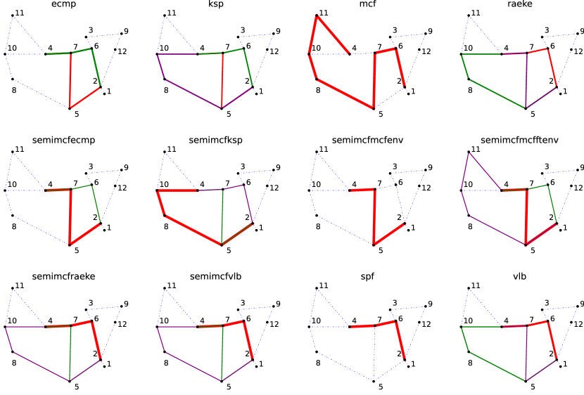
Figure 5: Case study: Abilene topology showing h4$\rightarrow$h2 paths used by different routing algorithms.

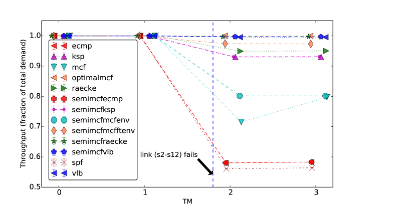
Figure 6: Case study: Throughput as fraction of total demand when link s2-s12 fails.

Case Study: How diverse are the paths chosen by different algorithms? A central thesis of this paper is that path selection algorithms have a large impact on the performance of traffic engineering schemes. We first explored exactly how different are the path sets selected by different algorithms. To visualizes the differences, we depict only the paths from a single source, PoP 4 (Denver), to a single destination, PoP 2 (Atlanta). We enforce a path budget of 3. In Figure 5, the red (thick) paths have the highest weights while the purple (thin) paths have the lowest weights. It is evident that the paths selected by different schemes may vary significantly on different runs.

While some paths are obvious (e.g., SPF picks the shortest path), others are sometimes surprising. For example, the “congestion-optimal” MCF routing scheme uses a very long path. Since MCF aims to minimize the maximum congestion, and not reduce latency, it may select long paths to accommodate other demands in the network.

Another interesting observation is that the path weights may differ significantly between oblivious schemes and their semi-oblivious alternatives, such as in Räcke and SemiMCF-Räcke. Moreover, even two semi-oblivious algorithms initialized with the same set of paths may differ in path weight. This is because when adapting rates to minimize congestion, the set of paths and demands between other pairs of PoPs are also considered. For example, SemiMCF-KSP assigns a higher weight to a longer path, because if it used the shorter one, a higher max-congestion would have occurred.

Case Study: Does path selection impact throughput when a link fails? To evaluate how path selection impacts performance in the presence of failures, we ran each algorithms under a simple failure scenario. We performed routing for four traffic matrices and failed the link connecting PoPs numbered 2 (Atlanta) and 12 (Washington) for traffic matrices 2 and 3. Figure 6 shows the fraction of total demand that could be delivered successfully. To recover from failure, each algorithm deployed local recovery. Since SPF selects only one path for any pair of PoPs, there is no way it can recover from failure and hence the throughput decreases drastically. On the other hand, schemes that have a large set of diverse paths, such as SemiMCF-Räcke, are more fault tolerant.

How does increased load impact throughput and loss? To evaluate how path selection affects performance under a variety of demands, we scaled the synthetic traffic matrices by a configurable factor $S$, for increasing values of $S$ from 1 to 2.5. The SWAN [24] paper reports that 0.4 is the maximum average congestion in real networks. For this reason, we define $S=1$ as corresponding to those traffic matrices for which the minimum max-congestion is 0.4. $S=2$ are matrices for which the minimum max-congestion is 0.8, etc. We measured the throughput, defined as fraction of the total demand, and congestion loss for all algorithms on the set of 9 topologies as described earlier. Figure 7 shows the expected trend that congestion loss increases with increasing scale. VLB, owing to the longer expected path lengths, starts experiencing maximum congestion loss as the network reaches capacity. For $S>2.5$, congestion loss is unavoidable as the minimum possible max-congestions reaches 1. We observe that:

1. MCF-based schemes perform the best as they are optimized to minimize max-congestion and achieve optimal performance.

2. SemiMCF-Räcke provides throughput close to optimal and better than all other non-MCF based schemes.

3. SemiMCFMCFFTEnv also takes failures into account and thus, it can select longer paths which do not minimize loss due to congestion.

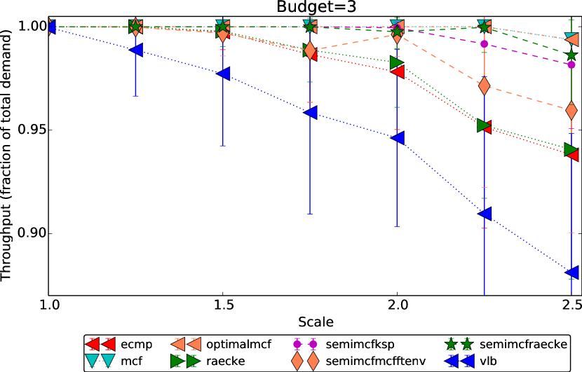
Figure 7: Impact of scaling demands by $S\in[1,2.5]$: throughput decreases and congestion loss increases.

How do link failures impact throughput and loss? Next, we measured the throughput and loss for the various algorithms as we: (i) increased the number of links ($\phi$) that can fail simultaneously from 0 to 3, (ii) varied the budget from 3 to 5, and (iii) increased the scale factor $S$ from 0.5 to 4. The failures are picked randomly, provided they don’t disconnect the network. We show the loss due to failure as a fraction of the total demand in figure 8. The y-axis is failure loss, and the x-axis is scale factor. Each graph shows the results for a fixed number of failed links. The budget was set to 3 for the 3 graphs in the top half , and it was set to 5 for the other 3.

Figure 8: Failure loss under different failure scenarios, scale, and budget. (a) budget=3 (b) budget=5

We observe the following:

1. In almost all scenarios, Räcke and SemiMCF-Räcke have the minimum loss due to failure.

2. Schemes that utilize the full budget, such as KSP, Räcke and VLB, experience less traffic loss.

3. As the number of failures increase, schemes that don’t use a diverse set of paths, such as SPF and MCF, react poorly.

How does prediction accuracy impact throughput? To evaluate the sensitivity to prediction error, we define a parameter $\epsilon$ as the factor used to perturb the weights of hosts while estimating demands based on the gravity model. We vary $\epsilon\in[0.00,0.80]$ to generate traffic matrices which are used as predicted traffic matrices by the routing algorithms. Figure 9 shows the effect on maximum congestion caused by this error in prediction. Oblivious routing schemes, as they don’t depend on predicted demands, don’t seem show any noticeable change with increasing prediction errors. However, algorithms which are MCF-based or SemiMCF-based (use predicted demands) show significant increase in congestion as prediction error increases. MCF starts with same maximum congestion as OptimalMCF at $\epsilon=0.0$, but quickly deteriorates with $\epsilon$.
Semi-oblivious schemes are more resilient compared to MCF as their base path set do not change for different $\epsilon$. Unlike MCF which can select a completely different set of paths for different $\epsilon$, these schemes perform rate adaptation over the same base path set as with $\epsilon=0.0$.

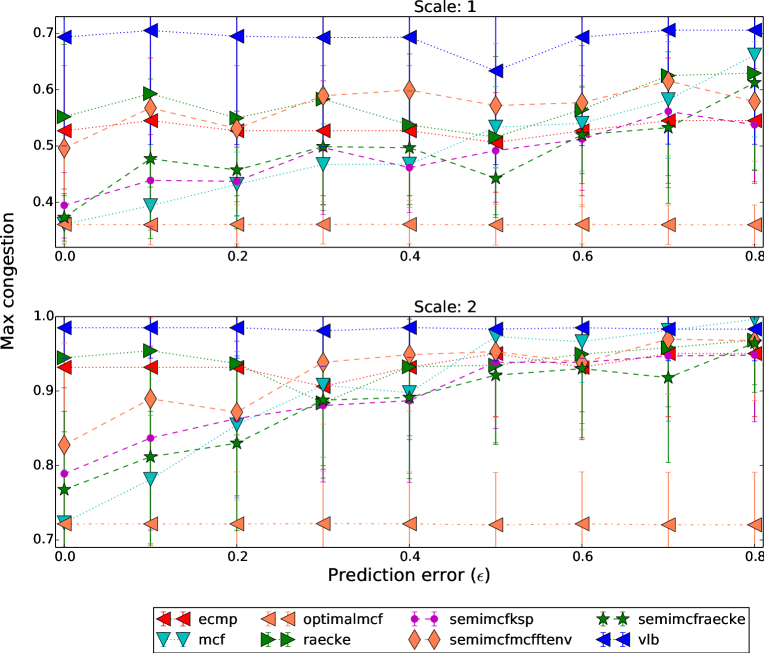
Figure 9: Resilience to error in demand prediction.

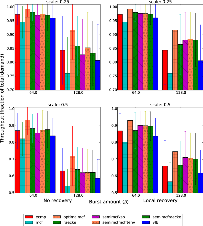
Figure 10: Effect of flash bursts on throughput. Semi-oblivious schemes improve with local recovery.

How do flash traffic bursts impact throughput? We compare the performance of different algorithms under flash bursts as we vary the amount of burst ($\beta$). We select a random sink hotspot (same for every algorithm) for every traffic matrix and measure the effect of congestion. Every algorithm has a flash recovery mechanism similar to “local recovery”. It is based on actual traffic matrix with a lag $\delta$. So, at time $t$, the algorithms have access to traffic observed at $t-\delta$. In our experiments, we use $\delta=8$. As the flash demands decay over time, in our experiments, all the algorithms perform local flash recovery (OptimalMCF does global recovery) every 200 time steps.

We measured the throughput as we increased the burst factor, $\beta$. Figure 10 shows the results. The graphs in the left column show the throughput without the recovery mechanism. The graphs on the right show the throughput with recovery. OptimalMCF is omniscient and uses actual traffic demands at the current time to compute a routing scheme by solving MCF. Thus, it achieves the best congestion ratio and high throughput. It easily outperforms other routing algorithms as long as there is spare capacity in the network (holds for $S\leq 2$). However, on enabling flash recovery, we find that most of the SemiMCF-based schemes improve in terms of throughput. MCF and SemiMCFMCFEnv deteriorate more than others as they are susceptible to inaccuracy in demand prediction. SemiMCF-Räcke and SemiMCFMCFFTEnv perform the best with local recovery. SemiMCFMCFFTEnv differs from MCF and SemiMCFMCFEnv because when it chooses a more diverse set of paths to be more resilient to failures, it automatically gets more path diversity to avoid bottlenecked links during flash crowds. The same reason holds for SemiMCF-Räcke.

How does path selection affect latency? Figure 11 shows the CDF of latency for three of the largest topologies we ran our experiments on. We see similar results with smaller topologies. We select the scale to be 2.5 so that the minimum max-congestion is 1.0, and we notice the effect of congestion.

1. SPF, KSP, ECMP and their SemiMCF-based variants use relatively shorter paths and thus have better 80-th percentile latency. But, since they don’t distribute traffic efficiently over less congested links, they incur higher tail latencies.

2. In contrast, SemiMCFMCFEnv and OptimalMCF can successfully deliver all the traffic but use longer paths.

3. SemiMCFRäcke occupies an attractive middle ground. It has similar 80-th percentile latency as the SPF, KSP and ECMP-based schemes. And it can also deliver the remaining 20% traffic using slightly longer paths as it distributes the traffic more efficiently.

4. SemiMCFMCFFTEnv trades off latency for more diverse (fault tolerant) but longer paths.

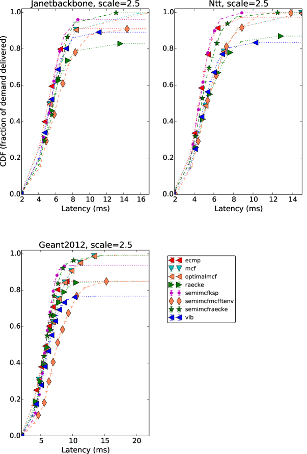
Figure 11: Latency CDF for different topologies.

How does path budget impact throughput and loss? SDN switches can only install a limited number of forwarding rules bound by their TCAM size. Routing schemes that use an excessive amount of rules may not be deployable in practice. For a network with $n$ vertices and $m$ edges, Räcke’s oblivious routing scheme can use $O(mn^{2}\log n)$ paths, or $O(m\log n)$ paths on an average between each pair of source and destination. Similarly, VLB and MCF can use up to $O(n)$ and $O(m)$ paths per pair, respectively. To address the limitations on number of forwarding rules, we enforce a budget on each algorithm. The budget restricts the number of paths used for each source and destination pair. Figure 12 shows the effect of the budget as demand scales. Initially, increasing the budget boosts throughput for SemiMCF-based schemes initialized with Räcke, MCF and VLB, as these schemes are able to spread traffic over a greater number of paths and able to minimize congestion. However, the improvement with increasing budget becomes negligible beyond a budget of 5. This shows that even though routing algorithms like Räcke’s need a lot of paths in theory to be efficient, they need only a reasonably small constant number of paths for real world WANs.

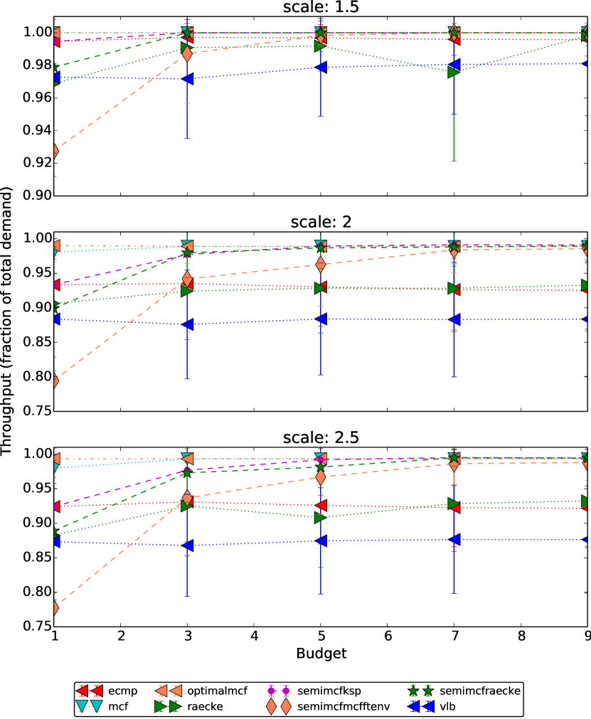
Figure 12: Throughput as path budget increases.

What are the operational overheads for different algorithms? We also measure various operational overheads such as churn, number of paths used and time to solve. Figure 13 show these overheads averaged over all the topologies. With respect to solver time, solving MCF over the entire set of possible paths is 2 orders of magnitude slower than SemiMcf based schemes where the base set of paths for each pair of source and destination is a small constant. LP-based solutions to MCF are very sensitive to slight changes in input. As a result with slight variations in traffic matrices over time, the set of paths used by MCF can vary greatly, resulting in high churn. When performing local recovery for failures, the base path set for all routing schemes, except OptimalMCF, didn’t change. Thus, they don’t incur any recovery churn. OptimalMCF solved MCF using the updated topology and thus has non-zero recovery churn. When measuring the number of paths used, we set budget to 3. Thus, most routing schemes ended up using their entire limit. However, algorithms like SPF and ECMP could use only a limited number of paths well within the budget. In our experiments, the number of paths chosen by MCF was close to 1 per pair on average.

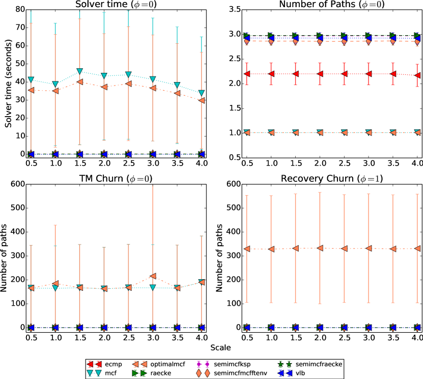
Figure 13: Various operational overheads associated with different routing schemes.

8 Related Work

There has been considerable interest in traffic engineering for wide-area networks, which we’ve already surveyed in Section 2. More broadly, there have been a number of recent systems for traffic engineering in the data center [2, 9, 33, 35, 27, 36, 42]. While clearly related, our work is focused on wide area networks, which face different requirements.

Several systems have proposed using randomized routing techniques. RouteBricks [5, 13] extends the basic Valiant load balancing algorithm to guard against packet-reordering, and to constant-degree graph topologies. Zhang-Shen and McKeown [45, 46] have proposed VLB for use with backbone networks, and show that the networks can guarantee 100% throughput for any traffic matrix, even in the event of link failures. Kodialam et al. [31, 30] proposed the use of oblivious routing in IP backbone networks. Applegate and Cohen [4] showed that, in practice, oblivious routing performed better than the worst-case theory predictions.

The discovery of oblivious routing schemes with polylogarithmic congestion in general networks by Räcke in 2002 [37] sparked significant interest in the theory community. The performance of Räcke’s original scheme was improved in a series of papers [10, 23] culminating in the optimal $O(\log n)$ scheme [38] used by our system. For any network topology, it is known how to compute an oblivious routing scheme with the optimal worst-case congestion ratio, in polynomial time, using the ellipsoid method [8] or interior point methods [4]. Oblivious routing schemes with a polylogarithmic, rather than logarithmic, congestion ratio can be computed in almost linear time [39]. Hajiaghayi et al. [21] derived improved bounds in models where the traffic matrix has independent random entries rather than worst-case entries.

9 Conclusion

Operators of wide-area networks face competing requirements when implementing a traffic engineering strategy. On the one hand, to improve operational efficiency, they seek to improve network utilization by distributing load evenly amongst capacitated links. On the other hand, to mitigate the overhead of network management, they seek to minimize the frequency and complexity of state changes on devices. The semi-oblivious traffic engineering (SOTE) scheme presented in this paper provides a balanced solution to the competing requirements of traffic engineering, while at the same time, simplifying the management infrastructure.

References

- [1] Historical Abilene Data. http://noc.net.internet2.edu/i2network/live-network-status/historical-abilene-data.html.
- [2] M. Al-Fares, S. Radhakrishnan, B. Raghavan, N. Huang, and A. Vahdat. Hedera: Dynamic Flow Scheduling for Data Center Networks. In NSDI, Apr. 2010.
- [3] M. Alizadeh, T. Edsall, S. Dharmapurikar, R. Vaidyanathan, K. Chu, A. Fingerhut, V. T. Lam, F. Matus, R. Pan, N. Yadav, and G. Varghese. CONGA: Distributed Congestion-aware Load Balancing for Datacenters. In SIGCOMM, pages 503–514, Aug. 2014.
- [4] D. Applegate and E. Cohen. Making Intra-domain Routing Robust to Changing and Uncertain Traffic Demands: Understanding Fundamental Tradeoffs. In SIGCOMM, pages 313–324, 2003.
- [5] K. Argyraki, S. Baset, B.-G. Chun, K. Fall, G. Iannaccone, A. Knies, E. Kohler, M. Manesh, S. Nedevschi, and S. Ratnasamy. Can Software Routers Scale? In PRESTO, pages 21–26, Aug. 2008.
- [6] S. Arora, E. Hazan, and S. Kale. The Multiplicative Weights Update Method: a Meta-Algorithm and Applications. TOC, 8(1):121–164, 2012.
- [7] B. Awerbuch and R. Khandekar. Greedy Distributed Optimization of Multi-Commodity Flows. Distributed Computing, 21(5):317–329, Nov. 2009.
- [8] Y. Azar, E. Cohen, A. Fiat, H. Kaplan, and H. Racke. Optimal Oblivious Routing in Polynomial Time. In 35th STOC, pages 383–388, 2003.
- [9] H. Ballani, P. Costa, T. Karagiannis, and A. Rowstron. Towards Predictable Datacenter Networks. In SIGCOMM, pages 242–253, Aug. 2011.
- [10] M. Bienkowski, M. Korzeniowski, and H. Räcke. A Practical Algorithm for Constructing Oblivious Routing Schemes. In 15th SPAA, pages 24–33, 2003.
- [11] M. Casado, T. Koponen, S. Shenker, and A. Tootoonchian. Fabric: A Retrospective on Evolving SDN. In HotSDN, pages 85–90, Aug. 2012.
- [12] W. Dally and B. Towles. Principles and Practices of Interconnection Networks. Morgan Kaufmann Publishers Inc., 2003.
- [13] M. Dobrescu, N. Egi, K. Argyraki, B.-G. Chun, K. Fall, G. Iannaccone, A. Knies, M. Manesh, and S. Ratnasamy. RouteBricks: Exploiting Parallelism to Scale Software Routers. In SOSP, pages 15–28, Oct. 2009.
- [14] J. Fakcharoenphol, S. Rao, and K. Talwar. A Tight Bound on Approximating Arbitrary Metrics by Tree Metrics. In 35th STOC, pages 448–455, 2003.
- [15] B. Fortz, J. Rexford, and M. Thorup. Traffic engineering with traditional IP routing protocols. IEEE Communications Magazine, 40(10):118–124, Oct. 2002.
- [16] B. Fortz and M. Thorup. Internet traffic engineering by optimizing OSPF weights. In 19th IEEE INFOCOM, volume 2, pages 519–528, 2000.
- [17] N. Garg and J. Könemann. Faster and Simpler Algorithms for Multicommodity Flow and Other Fractional Packing Problems. SICOMP, 37(2):630–652, May 2007.
- [18] P. B. Godfrey, I. Ganichev, S. Shenker, and I. Stoica. Pathlet Routing. SIGCOMM CCR, 39(4):111–122, Aug. 2009.
- [19] A. Greenberg, J. R. Hamilton, N. Jain, S. Kandula, C. Kim, P. Lahiri, D. A. Maltz, P. Patel, and S. Sengupta. VL2: A Scalable and Flexible Data Center Network. In SIGCOMM, pages 51–62, 2009.
- [20] Gurobi Optimization Inc. Gurobi optimizer.
- [21] M. Hajiaghayi, J. H. Kim, T. Leighton, and H. Räcke. Oblivious Routing in Directed Graphs with Random Demands. In 37th STOC, pages 193–201, 2005.
- [22] M. Hajiaghayi, R. Kleinberg, and T. Leighton. Semi-oblivious Routing: Lower Bounds. In SODA, pages 929–938, 2007.
- [23] C. Harrelson, K. Hildrum, and S. Rao. A Polynomial-time Tree Decomposition to Minimize Congestion. In 15th SPAA, pages 34–43, 2003.
- [24] C.-Y. Hong, S. Kandula, R. Mahajan, M. Zhang, V. Gill, M. Nanduri, and R. Wattenhofer. Achieving High Utilization with Software-Driven WAN. In SIGCOMM, pages 15–26, Aug. 2013.
- [25] The Internet Topology Zoo. http://www.topology-zoo.org.
- [26] S. Jain, A. Kumar, S. Mandal, J. Ong, L. Poutievski, A. Singh, S. Venkata, J. Wanderer, J. Zhou, M. Zhu, J. Zolla, U. Hölzle, S. Stuart, and A. Vahdat. B4: Experience with a Globally Deployed Software Defined WAN. In SIGCOMM, pages 3–14, Aug. 2013.
- [27] V. Jeyakumar, M. Alizadeh, D. Mazières, B. Prabhakar, A. Greenberg, and C. Kim. EyeQ: Practical Network Performance Isolation at the Edge. In NSDI, pages 297–312, Apr. 2013.
- [28] X. Jin, H. Liu, R. Gandhi, S. Kandula, R. Mahajan, J. Rexford, R. Wattenhofer, and M. Zhang. Dionysus: Dynamic Scheduling of Network Updates. In SIGCOMM, August 2014.
- [29] S. Kandula, D. Katabi, B. Davie, and A. Charny. Walking the tightrope: Responsive yet stable traffic engineering. In SIGCOMM, pages 253–264, Aug. 2005.
- [30] M. Kodialam, T. Lakshman, and S. Sengupta. Advances in oblivious routing of internet traffic. In Z. Liu and C. Xia, editors, Performance Modeling and Engineering, pages 125–146. Springer US, 2008.
- [31] M. Kodialam, T. V. Lakshman, J. B. Orlin, and S. Sengupta. Oblivious routing of highly variable traffic in service overlays and ip backbones. TON, 17(2):459–472, Apr. 2009.
- [32] A. Pathak, M. Zhang, Y. C. Hu, R. Mahajan, and D. Maltz. Latency Inflation with MPLS-based Traffic Engineering. In IMC, pages 463–472, 2011.
- [33] J. Perry, A. Ousterhout, H. Balakrishnan, D. Shah, and H. Fugal. Fastpass: A Centralized Zero-Queue Datacenter Network. In SIGCOMM, Chicago, IL, August 2014.
- [34] S. A. Plotkin, D. B. Shmoys, and E. Tardos. Fast Approximation Algorithms for Fractional Packing and Covering Problems. Mathematics of Operations Research, 20(2):257–301, Apr. 1995.
- [35] L. Popa, G. Kumar, M. Chowdhury, A. Krishnamurthy, S. Ratnasamy, and I. Stoica. FairCloud: Sharing the Network in Cloud Computing. In SIGCOMM, pages 187–198, Aug. 2012.
- [36] L. Popa, P. Yalagandula, S. Banerjee, J. C. Mogul, Y. Turner, and J. R. Santos. ElasticSwitch: Practical Work-Conserving Bandwidth Guarantees for Cloud Computing. In SIGCOMM, Aug. 2013.
- [37] H. Räcke. Minimizing Congestion in General Networks. In 43rd FOCS, pages 43–52, 2002.
- [38] H. Räcke. Optimal Hierarchical Decompositions for Congestion Minimization in Networks. In 40th STOC, pages 255–264, May 2008.
- [39] H. Räcke, C. Shah, and H. Täubig. Computing cut-based hierarchical decompositions in almost linear time. In SODA, pages 227–238, 2014.
- [40] M. Reitblatt, N. Foster, J. Rexford, C. Schlesinger, and D. Walker. Abstractions for Network Update. In SIGCOMM, pages 323–334, 2012.
- [41] M. Roughan, A. Greenberg, C. Kalmanek, M. Rumsewicz, J. Yates, and Y. Zhang. Experience in measuring backbone traffic variability: Models, metrics, measurements and meaning. In IMC, pages 91–92. ACM, 2002.
- [42] A. Shieh, S. Kandula, A. Greenberg, and C. Kim. Seawall: Performance Isolation for Cloud Datacenter Networks. In HotCloud, pages 1–8, June 2010.
- [43] M. Suchara, D. Xu, R. Doverspike, D. Johnson, and J. Rexford. Network architecture for joint failure recovery and traffic engineering. In SIGMETRICS, pages 97–108, 2011.
- [44] L. Valiant. A Scheme for Fast Parallel Communication. SICOMP, 11(2):350–361, 1982.
- [45] R. Zhang-Shen and N. McKeown. Designing a Predictable Internet Backbone with Valiant Load-Balancing. In 13th IEEE/ACM IWQoS, pages 178–192, 2005.
- [46] R. Zhang-Shen and N. Mckeown. Designing a Fault-Tolerant Network Using Valiant Load-Balancing. In 27th IEEE INFOCOM, Apr. 2008.