Constructing Scalar-Photon Three Point Vertex in Massless Quenched Scalar QED

Abstract

Non perturbative studies of Schwinger-Dyson equations (SDEs) require their infinite, coupled tower to be truncated in order to reduce them to a practically solvable set. In this connection, a physically acceptable ansatz for the three point vertex is the most favorite choice. Scalar quantum electrodynamics (sQED) provides a simple and neat platform to address this problem. The most general form of the three point scalar-photon vertex can be expressed in terms of only two independent form factors, a longitudinal and a transverse one. Ball and Chiu have demonstrated that the longitudinal vertex is fixed by requiring the Ward-Fradkin-Green-Takahashi identity (WFGTI), while the transverse vertex remains undetermined. In massless quenched sQED, we construct the transverse part of the non perturbative scalar-photon vertex. This construction (i) ensures multiplicative renormalizability (MR) of the scalar propagator in keeping with the Landau-Khalatnikov-Fradkin transformations (LKFTs), (ii) has the same transformation properties as the bare vertex under charge conjugation, parity and time reversal, (iii) has no kinematic singularities and (iv) reproduces one loop asymptotic result in the weak coupling regime of the theory.

I Introduction

Gauge theories of fundamental interactions have been the cornerstone of describing the physical world at the most basic level. Their enormous success primarily lies in the region where the coupling strength is small enough and the tools of perturbation theory are reliable. However, not all interesting phenomena can be accessed in this approximation scheme. In the non perturbative sector of quantum chromodynamics (QCD), two major phenomena emerge: 1) color confinement, and 2) dynamical chiral symmetry breaking (DCSB). For studying strongly interacting bound states, a reliable understanding of these phenomena is essential. However, it can be achieved solely through non perturbative techniques such as lattice QCD, SDEs, Dyson (1949); Schwinger (1951), chiral perturbation theory and effective quark models. Keeping this in mind, our interest is focussed on the study of the physically acceptable truncations of SDEs beyond perturbation theory.

SDEs are the fundamental equations of motion of any quantum field theory (QFT). They form an infinite set of coupled integral equations that relate the $n$-point Green function to the $(n+1)$-point function. As the simplest example, propagators are related to the three point vertices, the latter to the four point functions and so on, ad infinitum. As their derivation requires no assumption regarding the strength of the interaction, they are ideally suited for studying interactions like QCD, where one single theory has diametrically opposed perturbative and non perturbative facets in the ultraviolet and infrared regimes of momenta, respectively. Unfortunately, being an infinite set of coupled equations, they are intractable without some simplifying assumptions. Typically, in the non perturbative region, SDEs are truncated at the level of two-point Green functions (propagators). We must then use an ansatz for the full three point vertex. This has to be done carefully. Otherwise, solutions can be in conflict with some of the key features of a QFT, such as gauge invariance of physical observables and renormalizability of the divergent functions involved, thus jeopardizing the credibility of the truncation scheme employed.

In contrast with the complicated non abelian scenario of QCD, quantum electrodynamics (QED) has proved to be a good starting point in studying the non pertutbative regime of the SDEs. Better yet, in the absence of Dirac matrices, sQED can offer an even more attractive model to construct acceptable non perturbative $ans\ddot{a}tze$ for the vertices involved. In this article, we set out to construct a scalar-photon three point vertex which must comply with the following key criteria:

• It must satisfy the Ward-Fradkin-Green-Takahashi identity (WFGTI), Ward (1950); Green (1953); Takahashi (1957).

Just like in spinor QED and QCD, Ball and Chiu, Ball and Chiu (1980), provide the non perturbative form of the longitudinal three point vertex in sQED, which explicitly satisfies the WFGTI, Ward (1950); Green (1953); Takahashi (1957). We take it as our starting point.

• It must satisfy the local gauge covariance properties of the theory.

Note that although the WFGTI is a consequence of gauge invariance, it is insufficient to ensure the local gauge covariance relation of the scalar propagator. In order to ensure the latter, we demand the transverse part of the vertex to be constrained by the LKFTs, Landau and Khalatnikov (1956); Fradkin (1955); Johnson and Zumino (1959); Zumino (1960). The LKFTs are a well defined set of transformations which describe the response of the Green functions to an arbitrary gauge transformation. These transformations leave the SDEs and the WFGTI form-invariant and ensure chiral quark condensate is gauge invariant in spinor QED and QCD, a feature not guaranteed through satisfying WFGTI alone. Therefore, LKFTs potentially play an important role in guiding us toward an improved ansatz for the three point vertex and imposing gauge invariant chiral symmetry breaking, see for example Refs. Burden and Roberts (1993); Bashir (2000); Bashir and Raya (2002); Bashir and Delbourgo (2004); Bashir et al. (2006); Bashir and Raya (2007); Bashir et al. (2008a, 2009a); Aslam et al. (2015). More recently, these transformations have also been studied in the world line formalism, where we generalize LKFTs to arbitrary amplitudes in sQED, Ahmadiniaz et al. (2016).

The truncation scheme in preserving gauge invariance of observables has also been studied in simpler gauge theories such as QED3, e.g., Maris (1996); Bashir et al. (2002); Bashir and Raya (2002, 2005); Fischer et al. (2004); Lo and Swanson (2011). These works involve introducing constraints of gauge invariance in the truncations. In Ref. Fischer et al. (2004), it was shown that if one naively employed even the most sophisticated full Curtis-Pennington (CP) or Ball-Chiu (BC) vertices in different covariant gauges, they are not sufficient to ensure gauge invariant results for physical observables and the expected gauge covariance properties of the fermion propagator. However, in later articles Bashir and Raya (2007); Bashir et al. (2008b), the need to incorporate the LKFT correctly was emphasized in order to obtain gauge invariance of corresponding physical observables, such as the chiral quark condensate and the confinement-deconfinement phase transition as a function of the number of fermion flavors ($n_{f}$).

• It must ensure the multiplicative renormalizability (MR) of the two point propagator.

Studies in massless scalar and spinor QED as well as in QCD, demonstrate that the LKFT of the wavefunction renormalization implies an MR form of a power law, Bashir and Delbourgo (2004); Bashir and Raya (2002, 2004); Bashir et al. (2006); Aslam et al. (2015). We would like to reiterate that this solution can be reproduced only with an appropriate choice of the electron-photon three point vertex, as demonstrated first in Ref. Curtis and Pennington (1990). There have been a series of works, spanned over a couple of decades, which construct the electron-photon vertex, implementing the LKFT and MR of the electron propagator, Curtis and Pennington (1990, 1991); Dong et al. (1994); Bashir and Pennington (1994, 1996); Bashir et al. (1998, 1999, 2000); Kizilersu and Pennington (2009); Bashir et al. (2011a, 2012). In Ref. Bashir et al. (2012), MR was implemented for the fermion propagator and it simultaneously ensures the gauge invariance of the critical coupling, above which chiral symmetry is dynamically broken.

In this article, we impose the conditions of MR on the three point scalar-photon vertex in sQED. It involves an unknown function $W(x)$ of a dimensionless ratio $x$ of momenta, satisfying an integral constraint which guarantees the MR of the scalar propagator. In this construction, we assume that the transverse vertex has no dependence on the angle between the incoming and outgoing momenta of the scalar particle, an approximation which can be readily undone through defining an effective transverse vertex.

• It should reduce to its perturbation theory Feynman expansion in the limit of weak coupling.

A truncation of the complete set of SDEs, that maintains gauge invariance and MR of a gauge theory at every level of approximation, is perturbation theory. Physically meaningful solutions of the SDEs must agree with perturbative results in the weak coupling regime. We use one loop perturbative calculations as a guiding principle for the three point vertex, Kizilersu et al. (1995); Davydychev et al. (2001); Bashir et al. (2007). In our construction in terms of the function $W$ mentioned above, we explore how perturbation theory provides an additional constraint. Using a one loop calculation of the scalar-photon three point vertex presented in Refs. Bashir et al. (2007, 2009b), we derive a perturbative constraint on $W(x)$ to ${\cal{O}}(\alpha)$, in the leading logarithms approximation (LLA). We ensure that our non perturbative construction of the said vertex satisfies this constraint.

• It must have the same symmetry properties as the bare vertex under charge conjugation, parity and time reversal.

• One loop perturbation theory suggests that it should be free of any kinematic singularities. Following Ball and Chiu, Ball and Chiu (1980), we shall enforce this requirement.

The scalar-photon three point vertex $\Gamma^{\mu}(k,p)$ must be symmetric under the exchange of momenta $k$ and $p$. Moreover, we do not expect it to have kinematic singularities as $k^{2}\Rightarrow p^{2}$. We build these features into our construction.

The paper is organized as follows: in Section II we introduce the SDE for the massless scalar propagator in quenched sQED. We define the longitudinal and transverse parts of the scalar-photon vertex and simplify the SDE by performing angular integration. In Section III, we study the LKFT for the scalar propagator to obtain a non perturbative expression for the wavefunction renormalization which defines this propagator. We introduce and explain the concept of MR in Section IV. We deduce a power law solution for the wavefunction renormalization of the scalar propagator and compare it with the findings of the LKFT in Section III. Section V contains details of how we impose constraints of the LKFT and MR on the three point transverse scalar-photon vertex in terms of the function $W(x)$. In Section VI, we add additional constraints of one loop perturbation theory, symmetry properties and the lack of kinematic singularities. We also construct an explicit example of a non perturbative massless three point scalar-photon vertex. We present our conclusions and discussion in Section VII.

II The SDE for the Scalar Propagator

The explicit form of the sQED Lagrangian is:

$${\cal L}_{\rm sQED} = -\frac{1}{4}F_{\mu\nu}F^{\mu\nu}-\frac{1}{2\xi}\,\left(\partial^{\mu}A_{\mu}\right)^{2}+\left(\partial^{\mu}\varphi^{*}\right)\left(\partial_{\mu}\varphi\right)$$ (1)

$$- m^{2}\varphi^{*}\varphi-ie\left(\varphi^{*}\partial^{\mu}\varphi-\varphi\partial^{\mu}\varphi^{*}\right)A_{\mu}$$

$$+ 2e^{2}\varphi^{*}A^{\mu}\varphi A_{\mu}-\frac{\lambda}{4}(\varphi^{*}\varphi)^{2}\,.$$

The detailed derivation of the SDEs for relevant Green functions for this sQED Lagrangian already exists in literature, Binosi and Papavassiliou (2007). The SDE for the scalar propagator $S(k)$, in the quenched approximation, is shown in Fig. 1:

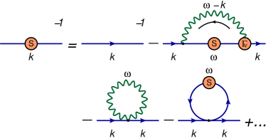
Figure 1: The SDE for the scalar propagator. The color-filled solid blobs labelled with $S$ and $\Gamma_{\nu}$ stand for the full scalar propagator and the full scalar-photon vertex, respectively. The dots ($\cdots$) represent all the diagrams whose contribution begins at the two loop level.

Mathematically, this is written as:

$$-iS^{-1}(k) = -iS_{0}^{-1}(k)$$ (2)

$$+ e^{2}\int_{M}{\frac{d^{4}\omega}{(2\pi)^{4}}(\omega+k)^{\mu}S(\omega)\Gamma^{\nu}(\omega,k)\Delta_{\mu\nu}(q)}$$

$$- e^{2}\int_{M}{\frac{d^{4}\omega}{(2\pi)^{4}}\Gamma^{\mu\nu}_{0}(k,-\omega,k,\omega)\Delta_{\mu\nu}(\omega)}$$

$$- \int_{M}{\frac{d^{4}\omega}{(2\pi)^{4}}S(\omega)\Gamma_{0}(k,\omega)}+\cdots\,,$$

where $e$ is the electromagnetic coupling, $q=\omega-k$, and the subscript $M$ indicates integration over the entire Minkowski space. $\Delta_{\mu\nu}(\omega)$ and $S_{0}(k)$ are the bare photon and scalar propagators. $S(k)$ is the full scalar propagator. For massless scalars, $S(k)$ can be expressed in terms of the so-called wavefunction renormalization $F(k^{2},\Lambda^{2})$, so that

$$S(k)=\frac{F(k^{2},\Lambda^{2})}{k^{2}}\,,$$ (3)

where $\Lambda$ is the ultraviolet cut-off used to regularize the divergent integrals involved. The bare scalar propagator is given by $S_{0}(k)=1/k^{2}$. The bare photon propagator is

$$\Delta_{\mu\nu}(q)=\frac{1}{q^{2}}\left[g_{\mu\nu}+(\xi-1)\frac{q_{\mu}q_{\nu}}{q^{2}}\right]\,,$$ (4)

and it remains unrenormalized in the quenched approximation. $\Gamma^{\mu\nu}_{0}(k,-\omega,k,\omega)=2ie^{2}g^{\mu\nu}$ and $\Gamma_{0}(k,\omega)=-i\lambda$ are the bare four point scalar-scalar-photon-photon and the four-scalar vertices, respectively. The last two diagrams of the gap equation, Eq. (2), will be referred to as the photon and the scalar bubble diagrams, in that order. $\Gamma^{\nu}(\omega,k)$ is the full three point scalar-photon vertex, for which we must make an ansatz in order to solve Eq. (2). The WFGTI for this vertex, i.e.,

$$q_{\mu}\Gamma^{\mu}(\omega,k)=S^{-1}(\omega)-S^{-1}(k)\,,$$ (5)

allows us to decompose it as a sum of longitudinal and transverse components, as suggested by Ball and Chiu, Ball and Chiu (1980):

$$\Gamma^{\mu}(\omega,k)=\Gamma_{L}^{\mu}(\omega,k)+\Gamma_{T}^{\mu}(\omega,k)\,.$$ (6)

The longitudinal part $\Gamma_{L}^{\mu}(\omega,k)$ satisfies the WFGTI, Eq. (5), by itself, and the transverse part $\Gamma_{T}^{\mu}(\omega,k)$, which remains completely undetermined, is naturally constrained by

$$q_{\mu}\Gamma_{T}^{\mu}(\omega,k)=0\,.$$ (7)

Moreover,

$$\Gamma_{T}^{\mu}(k,k)=0\,.$$ (8)

In order to satisfy the WFGTI in a manner free of kinematic singularities, we follow Ball and Chiu and write

$$\Gamma_{L}^{\mu}(\omega,k)=\frac{S^{-1}(\omega)-S^{-1}(k)}{\omega^{2}-k^{2}}(\omega+k)^{\mu}\,.$$ (9)

This construction implies that the ultraviolet divergences solely reside in the longitudinal part. Moreover, recall the following relations between the renormalized and bare quantities:

$$S^{R}(p)={\cal Z}_{2}^{-1}S(p)\,,\;\Gamma^{\mu}_{R}(k,p)={\cal Z}_{1}\Gamma^{\mu}(k,p)\,.$$ (10)

Thus, the form of the longitudinal vertex in Eq. (9) guarantees the relation ${\cal Z}_{1}={\cal Z}_{2}$. Consequently, the running of the coupling is dictated by the corrections to the photon propagator alone. In the approximation of quenched sQED, the coupling does not run. If we unquench the theory, it is easy to calculate ${\cal Z}_{3}$ and the running coupling constant with the well known expression:

$$\alpha(Q^{2})=\frac{\alpha(Q_{0}^{2})}{1-\left(\alpha(Q_{0}^{2})/12\pi\right){\rm ln}(Q^{2}/Q_{0}^{2})}\,.$$ (11)

The ultraviolet finite transverse vertex can be expanded out in terms of one unknown function $\tau(\omega^{2},k^{2},q^{2})$, Ball and Chiu (1980):

$$\Gamma_{T}^{\mu}(\omega,k)=\tau(\omega^{2},k^{2},q^{2})T^{\mu}(\omega,k)\,,$$ (12)

where

$$T^{\mu}(\omega,k)=\left(\omega\cdot q\right)k^{\mu}-\left(k\cdot q\right)\omega^{\mu}$$ (13)

is the transverse basis vector in the Minkowski space and fulfils Eqs. (7,8). To begin with, the form factor $\tau(\omega^{2},k^{2},q^{2})$ is an unconstrained scalar function (representing an $8$-fold simplification of the spinor QED/QCD case).

Following the non perturbative vertex construction/truncation of Refs. Ball and Chiu (1980); Bashir et al. (2007), our analysis ensures that gauge invariance (in terms of the WFGTI) for the scalar propagator and the scalar-photon vertex is satisfied. Within our truncation, another source of gauge non-invariance in the scalar propagator could be the lack of implementation of LKFT, a feature of the bare as well as BC vertices. We make sure that our ansatz for the transverse part satisfies this constraint non perturbatively. Photon propagator also has its Ward identity but we work throughout in the quenched approximation. Therefore, within the confines of our assumptions, it receives no corrections and hence the four point diagrams we have discarded do not affect the correct gauge invariance properties of the scalar propagator. They will be essential, for example, in ensuring the transversality of the photon propagator in unquenched sQED, not investigated in the present work. Furthermore, there are also restrictions of the gauge transformations on how the three point vertex is related to the four point vertex, constraining the form of the latter. In Ref.  Bashir et al. (2009b), two of the present authors exploited these constraints to carry out its non perturbative construction consistent with WFGTI which relates three point vertices to the four point ones. There is an undetermined part which is transverse to one or both the external photons, and needs to be evaluated through perturbation theory. They present in detail how the transverse part at the one loop order can be evaluated for completely general kinematics of momenta involved in covariant gauges and dimensions. In this article, our focus is on constraining the non perturbative three point scalar-photon vertex, capturing its key features, in particular its gauge covariance properties, its perturbative expansion in the LLA as well as the MR of the scalar propagator.

We make use of Eqs. (5, 6,9, 12,13) in the gap equation, i.e., Eq. (2), and then Wick rotate it to the Euclidean space to write:

$$\frac{1}{F(k^{2},\Lambda^{2})} = 1-\frac{\alpha}{4\pi^{3}}\frac{1}{k^{2}}\int_{E}{d^{4}\omega\frac{1}{q^{2}}\left\{\left[1-\frac{S(\omega)}{S(k)}\right]\right.}$$ (14)

$$\times\left[1+(\xi-1)\frac{\omega^{2}-k^{2}}{q^{2}}+2\frac{k^{2}}{\omega^{2}-k^{2}}\right.$$

$$\left.\left.+2\frac{\omega\cdot k}{\omega^{2}-k^{2}}\right]-2S(\omega)\tau(\omega^{2},k^{2},q^{2})\Delta^{2}\right\}\,,$$

where $\Delta^{2}=\left(\omega\cdot k\right)^{2}-\omega^{2}k^{2}$, $\alpha=e^{2}/4\pi$ is the bare coupling constant, and the subscript $E$ indicates integration over the whole Euclidean space. Note that we have neglected the photon and the scalar bubble diagrams as well as the diagrams whose contribution begins at the two loops level, since they do not contribute to leading logs in the one loop calculation, as we shall discuss later. At this stage, it appears impossible to proceed any further because of the dependence of $\tau$ on the angle between the incoming and outgoing momenta $\omega$ and $k$ of the scalar particle. We shall assume that the transverse vertex has no dependence on this angle, i.e., it is independent of $q^{2}$. Consequently, this vertex is only an effective one which will allow us to capture many key features of the theory in a simple manner. This assumption allows us to carry out the angular integration in Eq. (14). In this sense, we are calculating an effective transverse vertex. Note that it is easy to undo this independent angle approximation exactly. This has been explained and employed in Refs. Bashir et al. (1998, 2011b) for the case of spinor QED. Based upon the results found in these articles and our cross-check for sQED, we conclude that the qualitative implications of the ansatz of the three point scalar-photon vertex are insignificant, and hence we do not report corresponding findings.

The angular integration leads us to

$$\frac{1}{F(k^{2},\Lambda^{2})} = 1-\frac{\alpha}{4\pi}\int_{0}^{k^{2}}{d\omega^{2}\frac{\omega^{2}}{k^{2}}\left[1-\frac{S(\omega)}{S(k)}\right]}$$

$$\hskip 28.45274pt\times\left[\frac{(2-\xi)}{k^{2}}+\frac{1}{\omega^{2}-k^{2}}\left(2+\frac{\omega^{2}}{k^{2}}\right)\right]$$

$$-\frac{\alpha}{4\pi}\int_{k^{2}}^{\Lambda^{2}}{d\omega^{2}\left[1-\frac{S(\omega)}{S(k)}\right]\left\{\frac{3}{\omega^{2}-k^{2}}+\frac{\xi}{k^{2}}\right\}}$$

$$+\frac{\alpha}{8\pi}\int_{0}^{k^{2}}{d\omega^{2}\omega^{2}S(\omega)\tau(\omega^{2},k^{2})\left(\frac{\omega^{4}}{k^{4}}-3\frac{\omega^{2}}{k^{2}}\right)}$$

$$+\frac{\alpha}{8\pi}\int_{k^{2}}^{\Lambda^{2}}{d\omega^{2}\omega^{2}S(\omega)\tau(\omega^{2},k^{2})\left(\frac{k^{2}}{\omega^{2}}-3\right)}\,.$$

At this point, it is obvious that we require the knowledge of the form factor $\tau(\omega^{2},k^{2})$ to find the wavefunction renormalization $F(k^{2},\Lambda^{2})$. However, this problem can be inverted. The requirements of LKFT and the MR of $F(k^{2},\Lambda^{2})$ can tightly constrain the function $\tau(\omega^{2},k^{2})$. We would like to stress that these constraints will be valid only within our truncation scheme which consists of the set of assumptions and hypotheses we have detailed before. We study them in the next section.

III Scalar Propagator and LKFT

These transformations have the simplest structure in the Euclidean coordinate space. Therefore, we start by defining the Fourier transformations between the scalar propagators in coordinate and momentum spaces:

$${\cal S}_{E}(x;\xi) = \int\frac{d^{d}k}{(2\pi)^{d}}\ {\rm e}^{-i\mathbf{k}\cdot\mathbf{x}}\,S_{E}(k;\xi)\,,$$ (16)

$$S_{E}(k;\xi) = \int d^{d}x\ {\rm e}^{i\mathbf{k}\cdot\mathbf{x}}\,{\cal S}_{E}(x;\xi)\;.$$ (17)

Notice a slight modification of notation that we shall use in this section: $S(p)\Rightarrow S(p;\xi)$ for the sake of clarity. Moreover, we use the notation ${\cal S}$ for the propagator in the coordinate space in order to specify that its functional dependence is different from that of $S$, the same propagator in the momentum space. The subscript $E$ stands for the Euclidean space.

The LKFT relating the coordinate space scalar propagator in a given gauge $\xi_{0}$ to the one in an arbitrary covariant gauge $\xi$ reads:

$${\cal S}_{E}^{\rm LKFT}(x;\xi)={\cal S}_{E}(x;\xi_{0}){\rm e}^{-i[\Delta(0)-\Delta(x)]}\;,$$ (18)

where

$$\Delta(x) = -i(\xi-\xi_{0})e^{2}(\mu x)^{4-d}\int\frac{d^{d}k}{(2\pi)^{d}}\frac{{\rm e}^{-i\mathbf{k}\cdot\mathbf{x}}}{k^{4}}$$ (19)

$$= -\frac{i(\xi-\xi_{0})e^{2}}{16(\pi)^{d/2}}(\mu x)^{4-d}\Gamma\left(\frac{d}{2}-2\right)\;.$$

Here, $\mu$ is a mass scale introduced for dimensional purposes; it ensures that in every dimension $d$, the coupling $e$ is dimensionless. For the four dimensional case, we expand around $d=4-2\epsilon$ and use

$$\Gamma\left(-{\epsilon}\right) = -\frac{1}{\epsilon}-\gamma+{\cal O}(\epsilon)\;,$$

$$x^{\epsilon} = 1+\epsilon{\rm ln}x+{\cal O}(\epsilon^{2})\;.$$ (20)

Therefore,

$$\Delta(x)=i\frac{(\xi-\xi_{0})e^{2}}{16\pi^{2-\epsilon}}\Big{[}\frac{1}{\epsilon}+\gamma+2\ln\mu x+\mathcal{O}\,(\epsilon)\Big{]}\,.$$ (21)

Note that in the term proportional to $\ln x$, one cannot simply put $x=0$. Therefore, we need to introduce a cutoff scale $x_{\min}$. We then arrive at

$$\Delta(x_{\rm min})-\Delta(x)=-i\ln\left(\frac{x^{2}}{x_{\rm min}^{2}}\right)^{\nu}\,,$$ (22)

with $\nu={\alpha(\xi-\xi_{0})}/{(4\pi)}$. If we have the knowledge of the propagator in one gauge, we can transform it to any other gauge dictated by the LKFT:

$${\cal S}_{E}^{\rm LKFT}(x;\xi) = {\cal S}_{E}(x;\xi_{0})\,{\rm e}^{-i\big{(}\Delta(x_{\min})-\Delta(x)\big{)}}$$ (23)

$$= {\cal S}_{E}(x;\xi_{0})\,\Big{(}\frac{x^{2}}{x_{\rm min}^{2}}\Big{)}^{-\nu}\,.$$

Let us start from the tree level massive scalar propagator

$$S_{E}(k;\xi_{0})=-\frac{1}{k^{2}+m^{2}}\,.$$ (24)

Its Fourier transformation into the coordinate space is:

$${\cal S}_{E}(x;\xi_{0})=-\frac{m}{4\pi^{2}x}K_{1}(mx)\;,$$ (25)

where $K_{1}(mx)$ is the modified Bessel function of the second kind. The LKFT readily yields:

$${\cal S}_{E}^{\rm LKFT}(x;\xi) = -\frac{m}{4\pi^{2}x}K_{1}(mx)\left(\frac{x^{2}}{x^{2}_{\rm min}}\right)^{-\nu}\;.$$ (26)

We can Fourier transform this result back to the momentum space to get

$$S_{E}^{\rm LKFT}(k;\xi) = -\frac{1}{m^{2}}\left(\frac{m^{2}}{-\Lambda^{2}}\right)^{\nu}\Gamma(1-\nu)\Gamma(2-\nu)$$ (27)

$$\times\;_{2}F_{1}\left(1-\nu,2-\nu;2;-\frac{k^{2}}{m^{2}}\right)\,,$$

where we have made the identification $4/x_{\rm min}^{2}\rightarrow-\Lambda^{2}$. This is the non perturbative LKFT expression for the scalar propagator, starting from its knowledge at the tree level in the gauge $\xi_{0}$. To evaluate it in the massless limit, we make use of the identity

$${}_{2}F_{1}\left(a,b;c;z\right)=(1-z)^{-a}{}_{2}F_{1}\left(a,c-b;c;\frac{z}{z-1}\right)$$ (28)

to rewrite the scalar propagator as follows:

$$S_{E}^{\rm LKFT}(k;\xi)=-\left(\frac{1}{-\Lambda^{2}}\right)^{\nu}\Gamma(1-\nu)\Gamma(2-\nu)$$

$$\times\,(k^{2}+m^{2})^{\nu-1}\,_{2}F_{1}\left(1-\nu,\nu;2;-\frac{k^{2}}{k^{2}+m^{2}}\right)\,.$$ (29)

The massless limit now yields

$$S_{E}^{\rm LKFT}(k;\xi) = -\frac{1}{k^{2}}\;\frac{\Gamma(1-\nu)}{\Gamma(1+\nu)}\;\left(-\frac{k^{2}}{\Lambda^{2}}\right)^{\nu}\,.$$ (30)

This is a power law with exponent $\nu$. Expanding it out in the powers of coupling, retaining the leading logarithms and writing the result in the Minkowski space, we get:

$$S^{\rm LKFT}(k;\xi) = \frac{1}{k^{2}}\left[1+\,\frac{\alpha(\xi-\xi_{0})}{4\pi}\;{\rm ln}\left(\frac{k^{2}}{\Lambda^{2}}\right)\right]\,.$$ (31)

It implies

$$F^{\rm LKFT}(k^{2},\Lambda^{2}) = 1+\,\frac{\alpha(\xi-\xi_{0})}{4\pi}\;{\rm ln}\left(\frac{k^{2}}{\Lambda^{2}}\right)\,.$$ (32)

This result provides constraints on the transverse scalar-photon vertex through Eq. (LABEL:equation_for_F_with_effective_vertex). Before we set about exploiting this constraint, we would like to connect Eq. (32) with perturbation theory and MR of the scalar propagator in the next section.

IV Scalar Propagator and MR

MR of the scalar propagator requires the renormalized $F_{R}$ to be related to the unrenormalized $F$ through a multiplicative factor ${\cal Z}_{2}$ by

$$F_{R}(k^{2},\mu^{2})={\cal Z}_{2}^{-1}(\mu^{2},\Lambda^{2})F(k^{2},\Lambda^{2})\,,$$ (33)

where $\mu$ plays the role of an arbitrary renormalization scale. Within a truncation scheme which focusses only on logarithmic divergences, it is possible to write down the above functions as perturbative series involving terms of the form $\alpha^{n}\ln^{n}$ (the so called leading log terms). We should keep in mind that the sQED has features of a $\varphi^{4}$ scalar field theory as well as the spinor QED. It has both quadratic and logarithmic ultraviolet divergences. Our truncation scheme makes it resemble the spinor QED or QCD, problems of our eventual interest.

In the LLA, we then have

$$F(k^{2},\Lambda^{2}) = 1+\sum_{n=1}^{\infty}\alpha^{n}A_{n}\ln^{n}\left(\frac{k^{2}}{\Lambda^{2}}\right)\,,$$ (34)

$${\cal Z}_{2}^{-1}(\mu^{2},\Lambda^{2}) = 1+\sum_{n=1}^{\infty}\alpha^{n}B_{n}\ln^{n}\left(\frac{\mu^{2}}{\Lambda^{2}}\right)\,,$$ (35)

$$F_{R}(k^{2},\mu^{2}) = 1+\sum_{n=1}^{\infty}\alpha^{n}C_{n}\ln^{n}\left(\frac{k^{2}}{\mu^{2}}\right)\,.$$ (36)

(Note that the next to leading logs (NLL) are of the type $\alpha^{n}\ln^{n-1}$ and so on.) The MR condition, Eq. (33), requires

$$A_{n}=C_{n}=(-1)^{n}B_{n}=\frac{A_{1}^{n}}{n!}\,,$$ (37)

so that the functions $F$, $F_{R}$ and ${\cal Z}_{2}^{-1}$ obey a power law behavior. Thus the non perturbative solution of Eq. (33) for $F$ in the LLA is

$$F(k^{2},\Lambda^{2})=\left(\frac{k^{2}}{\Lambda^{2}}\right)^{\beta}\,,$$ (38)

where the anomalous dimension $\beta$ is unknown at the non pertubative level. This is in contrast with perturbation theory, where $\beta=\alpha A_{1}$ is obvious from Eq. (37). It is straightforward to calculate $A_{1}$ in one loop perturbation theory: taking the tree level values $\Gamma^{\nu}(\omega,k)=(\omega+k)^{\nu}$ and $S(\omega)=1/\omega^{2}$ in the gap equation, i.e., Eq. (2), we get, on Wick rotating it to the Euclidean space,

$$\frac{1}{F(k^{2},\Lambda^{2})} = 1-\frac{\alpha}{4\pi^{3}}\frac{1}{k^{2}}\int_{E}{\frac{d^{4}\omega}{\omega^{2}}\frac{(\omega+k)^{2}}{q^{2}}}$$ (39)

$$-\frac{\alpha}{4\pi^{3}}\frac{(\xi-1)}{k^{2}}\int_{E}{\frac{d^{4}\omega}{\omega^{2}}\frac{(\omega^{2}-k^{2})^{2}}{q^{4}}}\,.$$

Note that we have dropped the photon and the scalar bubble contributions as they do not contribute to the LLA. Angular integration of Eq. (39) yields

$$\frac{1}{F(k^{2},\Lambda^{2})} = 1+\frac{\alpha(\xi-3)}{4\pi}\int_{k^{2}}^{\Lambda^{2}}{\frac{d\omega^{2}}{\omega^{2}}}$$ (40)

$$+\frac{\alpha}{4\pi}\frac{(\xi-3)}{k^{4}}\int_{0}^{k^{2}}{d\omega^{2}\,\omega^{2}}-\frac{\alpha}{4\pi}\frac{\xi}{k^{2}}\int_{0}^{\Lambda^{2}}{d\omega^{2}}\,.$$

After carrying out the radial integration in the above Eq. (40), dropping the quadratic and quartic divergencies ($\Lambda^{2}$ and $\Lambda^{4}$) coming from the last two terms on the right hand side of Eq. (40) and conserving only the logarithmic divergence (as we are interested in the LLA), we have

$$F(k^{2},\Lambda^{2}) = 1+\frac{\alpha(\xi-3)}{4\pi}\ln\left(\frac{k^{2}}{\Lambda^{2}}\right)\,.$$ (41)

Comparing Eqs. (32,41), we deduce that $\xi_{0}=3$ is the correct choice for sQED till one loop order in perturbation theory. This is unlike the case of spinor QED, where Landau gauge $\xi=0$ works well for the same order of approximation.

Comparing expression (41) with the perturbative expansion (34) to one-loop order, we see that $A_{1}=(\xi-3)/4\pi$. Therefore, perturbation theory suggests that the anomalous dimension in (38) is

$$\beta=\frac{\alpha(\xi-3)}{4\pi}\,,$$ (42)

see also Delbourgo (1977, 2003); Kreimer (2004); Bashir et al. (2007). One can readily note that the power behavior of (38), with $\beta$ given in (42), is the solution of the following integral equation:

$$\frac{1}{F(k^{2},\Lambda^{2})}=1+\frac{\alpha(\xi-3)}{4\pi}\int_{k^{2}}^{\Lambda^{2}}{\frac{d\omega^{2}}{\omega^{2}}\frac{F(\omega^{2},\Lambda^{2})}{F(k^{2},\Lambda^{2})}}\,.$$ (43)

This term can be separated out in Eq. (LABEL:equation_for_F_with_effective_vertex) to impose the required condition of MR on the transverse form factor $\tau(\omega^{2},k^{2})$. This is what we study in the next section.

V The Transverse Vertex

Eq. (43) imposes the following restriction on the transverse vertex through Eq. (LABEL:equation_for_F_with_effective_vertex):

$$-2\int_{0}^{k^{2}}{d\omega^{2}\left\{\frac{3}{k^{2}}+\frac{(3-\xi)}{k^{2}}\frac{\omega^{2}}{k^{2}}+\frac{3}{\omega^{2}-k^{2}}\right.}$$

$$\left.+\frac{(\xi-3)}{k^{2}}\frac{F(\omega^{2},\Lambda^{2})}{F(k^{2},\Lambda^{2})}-\frac{3}{\omega^{2}-k^{2}}\frac{F(\omega^{2},\Lambda^{2})}{F(k^{2},\Lambda^{2})}\right\}$$

$$-2\int_{k^{2}}^{\Lambda^{2}}{d\omega^{2}\left\{\frac{3}{\omega^{2}-k^{2}}-\frac{3}{\omega^{2}-k^{2}}\frac{F(\omega^{2},\Lambda^{2})}{F(k^{2},\Lambda^{2})}+\frac{\xi}{k^{2}}\right\}}$$

$$+\int_{0}^{k^{2}}{d\omega^{2}F(\omega^{2})\tau(\omega^{2},k^{2})\left(\frac{\omega^{4}}{k^{4}}-3\frac{\omega^{2}}{k^{2}}\right)}$$

$$+\int_{k^{2}}^{\Lambda^{2}}{d\omega^{2}F(\omega^{2})\tau(\omega^{2},k^{2})\left(\frac{k^{2}}{\omega^{2}}-3\right)} = 0\,.$$

Recall that in the above equation, we have neglected the contributions of the photon and the scalar bubble diagrams since they do not contribute to the one loop LLA, Eq. (41). Introducing the variable $x$, where

$$x=\frac{\omega^{2}}{k^{2}} \forall \omega^{2}\in[0,k^{2}]\,,$$ (45)

$$x=\frac{k^{2}}{\omega^{2}} \forall \omega^{2}\in[k^{2},\Lambda^{2}]\,,$$ (46)

in Eq. (LABEL:transverse_vertex_RESTRICTION), the resulting restriction can be rewritten as

$$\int_{0}^{1}{dx\,W(x)}=0\,,$$ (47)

with

$$W(x) = -6x\frac{\left(1-x^{\beta}\right)}{x-1}+6x^{-1}\frac{\left(1-x^{-\beta}\right)}{x-1}+2\xi\left(1-x^{\beta}\right)$$ (48)

$$+\left(x-3\right)\left(x^{\beta}+x^{-2}\right)h(x)\,.$$

Note that we have again kept only those terms which contribute to the LLA. The lower limit $0$ of $x$ integration in Eq. (47) encodes the fact that we have taken $\Lambda^{2}\Rightarrow\infty$. This can be done with impunity as the all order logarithmic divergence has already been separated out to construct the MR solution for the wavefunction renormalization $F$. Moreover, we have introduced the definition

$$h(x)\equiv xk^{2}F(k^{2},\Lambda^{2})\tau(xk^{2},k^{2})\,,$$ (49)

which is a dimensionless function satisfying the property

$$h(x^{-1})=x^{\beta-1}h(x)\,,$$ (50)

with $\beta=(\xi-3)/4\pi$, as prescribed by Eq. (42). Employing Eq. (48) and the property in Eq. (50), we can write

$$W(x)-W(x^{-1}) = 4\left(x-1\right)\left(x^{\beta}+x^{-2}\right)h(x)$$ (51)

$$+6x\left(1-x^{\beta}\right)-6x^{-1}\left(1-x^{-\beta}\right)$$

$$+2\xi\left[\left(1-x^{\beta}\right)-\left(1-x^{-\beta}\right)\right]\,.$$

Taking $x=p^{2}/k^{2}$ in (51), and using the symmetry $\tau(p^{2},k^{2})=\tau(k^{2},p^{2})$, it is straightforward to derive the expression for $\tau(k^{2},p^{2})$ in terms of $W(x)$ and the wavefunction renormalization $F$. On Wick rotating it back to the Minkowski space, it acquires the following form:

$$\tau(k^{2},p^{2}) = -\frac{3}{2}\frac{1}{\left(k^{2}-p^{2}\right)}\left[\frac{1}{F(k^{2})}-\frac{1}{F(p^{2})}\right]$$ (52)

$$-\frac{\xi}{2}\frac{1}{\left(k^{2}-p^{2}\right)}\frac{F(k^{2})+F(p^{2})}{s(k^{2},p^{2})}\left[\frac{1}{F(k^{2})}-\frac{1}{F(p^{2})}\right]$$

$$+\frac{1}{4}\frac{1}{\left(k^{2}-p^{2}\right)}\frac{1}{s(k^{2},p^{2})}\left[W\left(\frac{k^{2}}{p^{2}}\right)-W\left(\frac{p^{2}}{k^{2}}\right)\right]\,,$$

where we have introduced $F(k^{2})\equiv F(k^{2},\Lambda^{2})$ as a simplifying notation. We also introduce the definition

$$s(k^{2},p^{2})=F(k^{2})\frac{k^{2}}{p^{2}}+F(p^{2})\frac{p^{2}}{k^{2}}\,.$$ (53)

In the transverse form factor, Eq. (52), the scalar structure $[1/F(k^{2})-1/F(p^{2})]$ appears, as first reported in spinor QED by Curtis and Pennington in Ref. Curtis and Pennington (1991). The exact form of the function $W$ remains unknown. Actually, there exists a whole family of $W$-functions satisfying the integral restriction, Eq. (47). However, for the sake of simplicity we can choose the trivial solution $W(x)=0$ for any dimensionless ratio $x$ of momenta. When substituted in Eq. (52), it leads to

$$\tau(k^{2},p^{2}) = -\frac{3}{2}\frac{1}{\left(k^{2}-p^{2}\right)}\left[\frac{1}{F(k^{2})}-\frac{1}{F(p^{2})}\right]$$ (54)

$$-\frac{\xi}{2}\frac{1}{\left(k^{2}-p^{2}\right)}\frac{F(k^{2})+F(p^{2})}{s(k^{2},p^{2})}\left[\frac{1}{F(k^{2})}-\frac{1}{F(p^{2})}\right]\,.$$

This vertex has already been calculated in one loop perturbation theory by Bashir et. al., Ref. Bashir et al. (2007), using dimensional regularization, in arbitrary gauge $\xi$ and dimensions $d$.

For the massless case, in dimension $d=4$, they report

$$\tau_{BCD}(k^{2},p^{2},q^{2})=$$

$$\frac{\alpha}{8\pi\Delta^{2}}\bigg{\{}(k^{2}+p^{2}-4k\cdot p)\left(k\cdot pJ_{0}+\ln\left(\frac{q^{4}}{p^{2}k^{2}}\right)\right)$$

$$+\frac{(k^{2}+p^{2})q^{2}-8p^{2}k^{2}}{p^{2}-k^{2}}\ln\left(\frac{k^{2}}{p^{2}}\right)$$

$$+(\xi-1)\left[k^{2}p^{2}J_{0}+\frac{2[k^{2}p^{2}+k\cdot p(k^{2}+p^{2})]}{k^{2}-p^{2}}\right]\ln\left(\frac{p^{2}}{k^{2}}\right)$$

$$+\frac{2k\cdot p}{k^{2}-p^{2}}\left[k^{2}\ln\left(\frac{q^{2}}{p^{2}}\right)-p^{2}\ln\left(\frac{q^{2}}{k^{2}}\right)\right]\bigg{\}}\,,$$ (55)

where

$$J_{0}=\frac{2}{i\pi^{2}}\int_{M}{d^{4}\omega\frac{1}{\omega^{2}\left(p-\omega\right)^{2}\left(k-\omega\right)^{2}}}\,,$$ (56)

with $q=k-p$. We now see if our proposal, Eq. (54), fares well against the constraints of this perturbative form factor, Eq. (55).

VI Perturbation Theory Constraints

In order to compare the vertex ansatz, Eq. (54), based upon multiplicative renormalizability, against its one loop perturbative form, Eq. (55), it is convenient to take the asymptotic limit $k^{2}\gg p^{2}$ of external momenta in the latter vertex. The resulting $\tau_{\rm BCD}$ in the LLA is

$$\tau^{\rm asym}_{\rm BCD}(k^{2},p^{2})\stackrel{{\scriptstyle k^{2}\gg p^{2}}}{{=}}-3\frac{\alpha}{4\pi}\frac{1}{k^{2}}\ln\left(\frac{k^{2}}{p^{2}}\right)\,.$$ (57)

Expectedly, it is independent of $q^{2}$ and hence we drop this dependence from its argument. Note that this expression is also independent of the covariant gauge parameter $\xi$. It is unlike spinor QED where the leading asymptotic vertex is proportional to $\xi$. For a numerical check, we define

$$\tilde{\tau}(x)=-\frac{k^{2}\,\tau(k^{2},xk^{2})}{\alpha\ln x}\,,$$ (58)

where $x=p^{2}/k^{2}$ and we have suppressed the $q^{2}$ dependence for notational simplification. Thus:

$$\tilde{\tau}^{\rm asym}_{\rm BCD}(x)=-\frac{3}{4\pi}\,.$$ (59)

In Fig. (2), we plot $\tilde{\tau}^{\rm asym}_{\rm BCD}(x)$ and $\tilde{\tau}_{\rm BCD}(x)$ as a function of $x$, the latter for different values of the gauge parameter $\xi$ and for a fixed value of $q^{2}$, chosen arbitrarily. In the asymptotic limit, all curves converge to a single value, as expected.

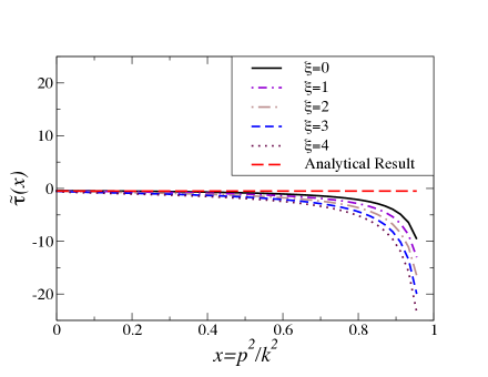
Figure 2: The analytical result, long dashed lines representing a constant value given in Eq. (59) for the asymptotic transverse form factor $\tilde{\tau}^{\rm asym}_{\rm BCD}(x)$, agrees with the numerical plot of $\tilde{\tau}_{\rm BCD}(x)$ obtained from Eq. (55) in the limit $x\rightarrow 0$ for different gauges and an arbitrarily chosen value of $q^{2}=-0.7GeV^{2}$.

Using the perturbative expression, Eq. (41), for $F(k^{2})$ in Eq. (54), and taking the asymptotic limit $k^{2}\gg p^{2}$, we have

$$\tau^{\rm asym}(k^{2},p^{2})\stackrel{{\scriptstyle k^{2}\gg p^{2}}}{{=}}\frac{3}{2}\frac{\alpha}{4\pi}\frac{\left(\xi-3\right)}{k^{2}}\ln\left(\frac{k^{2}}{p^{2}}\right)$$ (60)

in the LLA. Note that the transverse form factors, Eqs. (57) and (60) have the functional form $({1}/{k^{2}})\ln({k^{2}}/{p^{2}})$. Furthermore, they are the same in the Feynman gauge ($\xi=1$). In order for them to be the same in an arbitrary gauge $\xi$, we must seek a non-trivial $W$-function in Eq. (52), still satisfying the restriction in Eq (47), so that the corresponding perturbative vertex is consistent with Eq. (57) in the asymptotic limit $k^{2}\gg p^{2}$. Perhaps the simplest such choice for $W$ is

$$W\left(\frac{k^{2}}{p^{2}}\right) = \lambda\,\frac{k^{2}}{p^{2}}\ln\left(\frac{k^{2}}{p^{2}}\right)+\frac{\lambda}{2}\,\frac{k^{2}}{p^{2}}\,,$$ (61)

with $\lambda=-3\alpha(\xi-1)/2\pi$. In the Feynman gauge ($\xi=1$) $W=0$, i.e., there is no necessity of a non-trivial $W$-function since both perturbative vertices, Eqs. (57) and (60) are already the same. Note that the second term in the right hand side of Eq. (61) is a convenient term to ensure MR of the scalar propagator. It drops out in the LLA. Using the variable $x=k^{2}/p^{2}$ in Eq. (61), we have

$$W(x)=\lambda\,x\ln x+\frac{\lambda}{2}\,x\,,$$ (62)

so that the restriction in Eq. (47) is trivially satisfied. Using the choice in Eq. (61) for $W$ in the vertex, Eq. (52), we can finally define the transverse form factor as:

$$\tau(k^{2},p^{2}) = -\frac{3}{2}\frac{1}{\left(k^{2}-p^{2}\right)}\left[\frac{1}{F(k^{2})}-\frac{1}{F(p^{2})}\right]$$ (63)

$$-\frac{\xi}{2}\frac{1}{\left(k^{2}-p^{2}\right)}\frac{F(k^{2})+F(p^{2})}{s(k^{2},p^{2})}\left[\frac{1}{F(k^{2})}-\frac{1}{F(p^{2})}\right]$$

$$-\frac{\left(\xi-1\right)}{\left(k^{2}-p^{2}\right)s(k^{2},p^{2})}\frac{3\alpha}{8\pi}\left[\frac{k^{2}}{p^{2}}+\frac{p^{2}}{k^{2}}\right]\ln\left(\frac{k^{2}}{p^{2}}\right)\,.$$

Note that the Eqs. (6,9,12,63) define our full vertex ansatz. It ensures the following key features of sQED:

	Structure	MR	$\beta$
Bare Vertex	$(k+\omega)^{\mu}$	No
BC Vertex	$[(S^{-1}(\omega)-S^{-1}(k))(\omega+k)^{\mu}]/(\omega^{2}-k^{2})$	No
This work	$\Gamma_{T}^{\mu}(\omega,k)=\Gamma_{L}^{\mu}(\omega,k)+\tau(\omega^{2},k^{2},q^{2})[\left(\omega\cdot q\right)k^{\mu}-\left(k\cdot q\right)\omega^{\mu}]$	Yes	$\alpha(\xi-3)/4\pi$

Table 1: We compare different vertex ansätze: Bare, BC and our proposal, the last being the only vertex satisfying the constraints of LKFT and MR. The last column gives the value of the exponent $\beta$ of the multiplicatively renormalizable wave-function renormalization in Eq. (38).

• It satisfies the WFGTI by construction, Ward (1950); Green (1953); Takahashi (1957).

• It guarantees the LKFT property of the scalar propagator and can be checked by employing it in its SDE. In other words, it ensures the multiplicative renormalizability (MR) of the two point scalar propagator.

• It reduces to its one loop perturbation theory Feynman expansion in the limit of small coupling and asymptotic values of momenta $k^{2}\gg p^{2}$.

• It has the same symmetry properties as the bare vertex under charge conjugation, parity and time reversal, which imply symmetry under $k\leftrightarrow p$.

• It is free of any kinematic singularities when $k^{2}\Rightarrow p^{2}$, i.e.,

  $$\underset{k^{2}\Rightarrow p^{2}}{\rm lim}\;(k^{2}-p^{2})\,\tau(k^{2},p^{2})=0\,.$$ (64)

An important thing to note is that in the ansatz for $W$ given in Eq. (62), MR condition is satisfied independently of the value of the parameter $\lambda$. Moreover, $\lambda$ is tied to the anomalous dimensions $\beta$. To the first order in $\alpha$, we have

$$\beta=-\frac{\lambda}{6}-\frac{\alpha}{2\pi}\,.$$ (65)

The NLL and subsequent logs can be obtained by writing out:

$$\beta=\frac{\alpha(\xi-3)}{4\pi}+c_{2}{\cal O}(\alpha^{2})+c_{3}{\cal O}(\alpha^{3})+\cdots\,.$$ (66)

Note that the scalar and tensor vertices present in the SDE of the scalar propagator, Eq. (2), can start contributing at the NLL and hence are required to determine the values of the coefficients $c_{i},i\geq 2$. However, the NLL and constraints from subsequent orders can be absorbed in our ansatz for the effective vector vertex. Practically, this is achieved by a new definition for $\lambda$ without affecting the MR condition. Therefore, the procedure outlined above can easily accommodate the NLL, NNLL and so on. We only require $c_{i}$ for $i=2,3,\cdots$, which are provided by increasing orders of perturbation theory, see for example Capper et al. (1985).

Note that the kinematic dependence of the vertex on $q^{2}$ plays no role asymptotically and the standard analysis proceeds without reference to it. On the infrared domain, however, the kinematic dependence on $q^{2}$ may be important. Our vertex has this pitfall but its simplicity is reason enough for us to ignore this dependence.

Finally, in Table 1, we compare different vertex ansätze as regards the correct behavior of the scalar propagator under LKFT and MR. Neither the bare vertex nor the BC vertex yield an MR solution. Our proposal is the only one satisfying this constraint with the exponent of the wavefunction renormalization in agreement with the all order LLA in perturbation theory.

VII Conclusions

In the massless quenched sQED, we have derived a practical and easy to implement constraint of multiplicative renormalizability on the three point scalar-photon vertex. It leads to a family of these vertices in terms of a constrained dimensionless function $W(x)$. It has a remarkably simple non perturbative integral restriction:

$$\int_{0}^{1}{dx\,W(x)}=0\,,$$

which guarantees the multiplicative renormalizability of the scalar propagator to all orders in perturbation theory. We further pin down $W$ through the constraints of one loop perturbation theory in the asymptotic limit, lack of kinematic singularities and the imposition of discrete symmetries. Finally, we construct a simple example ensuring all these key features of the sQED. Though it is an example from one of the simplest QFTs, it provides a systematic procedure for constructing a three point function in terms of the corresponding two point function. This method is general and can be implemented in a similar manner to unquenched sQED as well as any other QFT of interest. In this connection, we would like to comment that an extension to the case of unquenched sQED is algebraically rather involved. For example for spinor QED, its unquenched version has been investigated in Kizilersu and Pennington (2009). It involves the constraints of MR both on the fermion and photon propagators for massless fermions. However, the fact remains that in the limit of $n_{f}\rightarrow 0$, one recuperates the quenched QED results.

Another obvious and straightforward extension of this work is to apply the same formalism to QCD and constrain the quark-gluon vertex through the requirements of MR. It will supplement the earlier works to improve our understanding of this three point function on lattice, Skullerud et al. (2003, 2005); Kizilersu et al. (2007), as well as through continuum methods, Chang and Roberts (2009); Qin et al. (2013); Rojas et al. (2013). We naturally expect the quark-gluon vertex to invoke more W-functions because the transverse part of this three point vertex is a lot richer than the one in sQED with eight independent transverse vectors as compared to only one for the latter. This work is currently in progress.

Acknowledgements: We are grateful to Sixue Qin, Robert Delbourgo and Alfredo Raya for helpful discussions. This work was partly supported by CIC, CONACyT and PRODEP grants.

References

- Dyson (1949) F. Dyson, Phys.Rev. 75, 1736 (1949).
- Schwinger (1951) J. S. Schwinger, Proc.Nat.Acad.Sci. 37, 452 (1951).
- Ward (1950) J. C. Ward, Phys.Rev. 78, 182 (1950).
- Green (1953) H. Green, Proc.Phys.Soc. A66, 873 (1953).
- Takahashi (1957) Y. Takahashi, Nuovo Cim. 6, 371 (1957).
- Ball and Chiu (1980) J. S. Ball and T.-W. Chiu, Phys.Rev. D22, 2542 (1980).
- Landau and Khalatnikov (1956) L. Landau and I. Khalatnikov, Sov.Phys.JETP 2, 69 (1956).
- Fradkin (1955) E. Fradkin, Zh.Eksp.Teor.Fiz. 29, 258 (1955).
- Johnson and Zumino (1959) K. Johnson and B. Zumino, Phys.Rev.Lett. 3, 351 (1959).
- Zumino (1960) B. Zumino, J.Math.Phys. 1, 1 (1960).
- Burden and Roberts (1993) C. J. Burden and C. D. Roberts, Phys. Rev. D47, 5581 (1993), eprint hep-th/9303098.
- Bashir (2000) A. Bashir, Phys.Lett. B491, 280 (2000).
- Bashir and Raya (2002) A. Bashir and A. Raya, Phys.Rev. D66, 105005 (2002), eprint hep-ph/0206277.
- Bashir and Delbourgo (2004) A. Bashir and R. Delbourgo, J.Phys. A37, 6587 (2004), eprint hep-ph/0405018.
- Bashir et al. (2006) A. Bashir, L. Gutierrez-Guerrero, and Y. Concha-Sanchez, AIP Conf.Proc. 857, 279 (2006).
- Bashir and Raya (2007) A. Bashir and A. Raya, Few Body Syst. 41, 185 (2007), eprint hep-ph/0511291.
- Bashir et al. (2008a) A. Bashir, A. Raya, and S. Sanchez-Madrigal, J.Phys. A41, 505401 (2008a), eprint 0811.3050.
- Bashir et al. (2009a) A. Bashir, A. Raya, S. Sanchez-Madrigal, and C. Roberts, Few Body Syst. 46, 229 (2009a), eprint 0905.1337.
- Aslam et al. (2015) M. J. Aslam, A. Bashir, and L. Gutierrez-Guerrero (2015), eprint 1505.02645.
- Ahmadiniaz et al. (2016) N. Ahmadiniaz, A. Bashir, and C. Schubert, Phys. Rev. D93, 045023 (2016), eprint 1511.05087.
- Maris (1996) P. Maris, Phys. Rev. D54, 4049 (1996), eprint hep-ph/9606214.
- Bashir et al. (2002) A. Bashir, A. Huet, and A. Raya, Phys. Rev. D66, 025029 (2002), eprint hep-ph/0203016.
- Bashir and Raya (2005) A. Bashir and A. Raya, Nucl. Phys. B709, 307 (2005), eprint hep-ph/0405142.
- Fischer et al. (2004) C. S. Fischer, R. Alkofer, T. Dahm, and P. Maris, Phys. Rev. D70, 073007 (2004), eprint hep-ph/0407104.
- Lo and Swanson (2011) P. M. Lo and E. S. Swanson, Phys. Rev. D83, 065006 (2011), eprint 1010.1244.
- Bashir et al. (2008b) A. Bashir, A. Raya, I. C. Cloet, and C. D. Roberts, Phys. Rev. C78, 055201 (2008b), eprint 0806.3305.
- Bashir and Raya (2004) A. Bashir and A. Raya (2004), eprint hep-ph/0411310.
- Curtis and Pennington (1990) D. Curtis and M. Pennington, Phys.Rev. D42, 4165 (1990).
- Curtis and Pennington (1991) D. Curtis and M. Pennington, Phys.Rev. D44, 536 (1991).
- Dong et al. (1994) Z.-h. Dong, H. J. Munczek, and C. D. Roberts, Phys.Lett. B333, 536 (1994), eprint hep-ph/9403252.
- Bashir and Pennington (1994) A. Bashir and M. Pennington, Phys.Rev. D50, 7679 (1994), eprint hep-ph/9407350.
- Bashir and Pennington (1996) A. Bashir and M. Pennington, Phys.Rev. D53, 4694 (1996), eprint hep-ph/9510436.
- Bashir et al. (1998) A. Bashir, A. Kizilersu, and M. Pennington, Phys.Rev. D57, 1242 (1998), eprint hep-ph/9707421.
- Bashir et al. (1999) A. Bashir, A. Kizilersu, and M. Pennington (1999), eprint hep-ph/9907418.
- Bashir et al. (2000) A. Bashir, A. Kizilersu, and M. R. Pennington, Phys.Rev. D62, 085002 (2000), eprint hep-th/0010210.
- Kizilersu and Pennington (2009) A. Kizilersu and M. Pennington, Phys.Rev. D79, 125020 (2009), eprint 0904.3483.
- Bashir et al. (2011a) A. Bashir, C. Calcaneo-Roldan, L. Gutierrez-Guerrero, and M. Tejeda-Yeomans, Phys.Rev. D83, 033003 (2011a), eprint 1101.5458.
- Bashir et al. (2012) A. Bashir, R. Bermudez, L. Chang, and C. Roberts, Phys.Rev. C85, 045205 (2012), eprint 1112.4847.
- Kizilersu et al. (1995) A. Kizilersu, M. Reenders, and M. R. Pennington, Phys. Rev. D52, 1242 (1995), eprint hep-ph/9503238.
- Davydychev et al. (2001) A. I. Davydychev, P. Osland, and L. Saks, Phys. Rev. D63, 014022 (2001), eprint hep-ph/0008171.
- Bashir et al. (2007) A. Bashir, Y. Concha-Sanchez, and R. Delbourgo, Phys.Rev. D76, 065009 (2007), eprint 0707.2434.
- Bashir et al. (2009b) A. Bashir, Y. Concha-Sanchez, R. Delbourgo, and M. Tejeda-Yeomans, Phys.Rev. D80, 045007 (2009b), eprint 0906.4164.
- Binosi and Papavassiliou (2007) D. Binosi and J. Papavassiliou, JHEP 03, 041 (2007), eprint hep-ph/0611354.
- Bashir et al. (2011b) A. Bashir, A. Raya, and S. Sanchez-Madrigal, Phys. Rev. D84, 036013 (2011b), eprint 1108.4748.
- Delbourgo (1977) R. Delbourgo, J. Phys. A10, 1369 (1977).
- Delbourgo (2003) R. Delbourgo, J. Phys. A36, 11697 (2003), eprint hep-th/0309047.
- Kreimer (2004) D. Kreimer, Nucl. Phys. Proc. Suppl. 135, 238 (2004), [,238(2004)], eprint hep-th/0407016.
- Capper et al. (1985) D. M. Capper, D. R. T. Jones, and A. T. Suzuki, Z. Phys. C29, 585 (1985).
- Skullerud et al. (2003) J. I. Skullerud, P. O. Bowman, A. Kizilersu, D. B. Leinweber, and A. G. Williams, JHEP 04, 047 (2003), eprint hep-ph/0303176.
- Skullerud et al. (2005) J.-I. Skullerud, P. O. Bowman, A. Kizilersu, D. B. Leinweber, and A. G. Williams, Nucl. Phys. Proc. Suppl. 141, 244 (2005), [,244(2004)], eprint hep-lat/0408032.
- Kizilersu et al. (2007) A. Kizilersu, D. B. Leinweber, J.-I. Skullerud, and A. G. Williams, Eur. Phys. J. C50, 871 (2007), eprint hep-lat/0610078.
- Chang and Roberts (2009) L. Chang and C. D. Roberts, Phys. Rev. Lett. 103, 081601 (2009), eprint 0903.5461.
- Qin et al. (2013) S.-X. Qin, L. Chang, Y.-X. Liu, C. D. Roberts, and S. M. Schmidt, Phys.Lett. B722, 384 (2013), eprint 1302.3276.
- Rojas et al. (2013) E. Rojas, J. de Melo, B. El-Bennich, O. Oliveira, and T. Frederico, JHEP 1310, 193 (2013), eprint 1306.3022.