Multilogarithmic velocity renormalization in graphene

Abstract

We reexamine the effect of long-range Coulomb interactions on the quasiparticle velocity in graphene. Using a nonperturbative functional renormalization group approach with partial bosonization in the forward scattering channel and momentum transfer cutoff scheme, we calculate the quasiparticle velocity, $v(k)$, and the quasiparticle residue, $Z$, with frequency-dependent polarization. One of our most striking results is that $v(k)\propto\ln[C_{k}(\alpha)/k]$ where the momentum- and interaction-dependent cutoff scale $C_{k}(\alpha)$ vanishes logarithmically for $k\rightarrow 0$. Here $k$ is measured with respect to one of the charge neutrality (Dirac) points and $\alpha=2.2$ is the strength of dimensionless bare interaction. Moreover, we also demonstrate that the so-obtained multilogarithmic singularity is reconcilable with the perturbative expansion of $v(k)$ in powers of the bare interaction.

I Introduction

In the last decade, due to the exceptional physical properties Geim07 ; Castroneto09 ; Dassarma11 of graphene, the two-dimensional all carbon material has been envisaged as a natural candidate for various low-dimensional device applications Schwierz10 ; Bonaccorso10 ; Avouris10 . But certain characteristics of electron-electron interactions in graphene Kotov12 still remain unsettled, as explained below, despite many sincere attempts to unravel the significance of interaction effects Gonzalez94 ; Gonzalez99 ; Herbut06 ; Bostwick07 ; Dassarma07 ; Novoselov07 ; Mishchenko07 ; Vafek07 ; Son07 ; Vafek08 ; Herbut08 ; Drut08 ; Foster08 ; Kotov08 ; Elias11 ; Sharma12 ; Chae12 ; Barnes14 ; Hofmann14 ; Bauer15 .

An important manifestation of many-body interactions in freely suspended graphene was observed in the quasiparticle velocity, $v(k)$, which was experimentally Elias11 shown to acquire a logarithmic enhancement close to one of its charge neutrality (Dirac) points. Such a behavior was found to be comparable to the first-order perturbation theory Gonzalez94 , i.e.,

$$\frac{v(k)}{v_{F}}\approx 1+\frac{\alpha}{4}\ln\left(\frac{\Lambda_{0}}{k}\right),$$ (1)

with $\Lambda_{0}$ being the ultraviolet cutoff of the order of inverse lattice spacing of the underlying honeycomb lattice and the momentum $k$ is measured relative to the Dirac point. Here $\alpha=e^{2}/v_{F}\approx 2.2$ is the strength of dimensionless bare interaction in vacuum with $e$ being the electron charge and $v_{F}$ is the bare Fermi velocity at the Dirac points. Since $\alpha$ is of order unity, it signifies the failure of perturbation theory, i.e., expansion of $v(k)$ in powers of $\alpha$, in explaining the experimental results. Due to the lack of dielectric and conduction screening in freely standing and undoped graphene the theories based on the random phase approximation (RPA) Hofmann14 remain doubtful. Moreover, large-$N$ approximation Gonzalez99 ; Herbut06 ; Son07 ; Drut08 ; Foster08 , an expansion in the inverse number $N$ of fermionic flavors, is questionable because in the physically relevant case of graphene $N=4$ is rather small.

Recently, Barnes et al. Barnes14 demonstrated the breakdown of perturbation theory (which, however, does not imply nonrenormalizability of the underlying field theory) and showed that the direct expansion of $v(k)$ in powers of $\alpha$ generates a series involving all powers of logarithms,

$$\frac{v(k)}{v_{F}} = 1+\sum_{n=1}^{\infty}F_{n}(\alpha)\left[\ln\left(\frac{\Lambda_{0}}{k}\right)\right]^{n},$$ (2)

where the interaction-dependent coefficients have the following expansion in powers of $\alpha$ :

$$F_{1}(\alpha) = f_{1}^{(1)}\alpha+f_{1}^{(2)}\alpha^{2}+f_{1}^{(3)}\alpha^{3}+{\cal{O}}(\alpha^{4}),$$ (3)

$$F_{n}(\alpha) = f_{n}^{(n+1)}\alpha^{n+1}+{\cal{O}}(\alpha^{n+2}),\mbox{ for $n\geq 2$}.$$ (4)

The superscripts correspond to the powers of $\alpha$ and hence to the number of loops in the corresponding Feynman diagrams. The authors of Ref. [Barnes14, ] also pointed out that to order $\alpha^{n}$, $n\geq 2$, the perturbation series of $v(k)$ contains all powers $[\ln(\Lambda_{0}/k)]^{m}$ of the basic logarithm in the range $m=1,\ldots,n-1$. Thus, from three-loop order onwards, the higher logarithmic powers start appearing in the perturbative expansion. The numerical value of the one-loop coefficient is known to be $f_{1}^{(1)}=1/4$ but for the two-loop coefficient $f^{(2)}_{1}$ there exist conflicting results Mishchenko07 ; Vafek08 ; Sharma12 ; Barnes14 . It is clear, however, that the above series in powers of logarithms cannot be resumed to a power law. Moreover, the perturbative expansion in Eq. (2) seems to be incompatible with previous renormalization group (RG) calculations Gonzalez94 ; Bauer15 as well as with resummation schemes based on the RPA Hofmann14 which did not find higher powers of $\ln(\Lambda_{0}/k)$. This is a clear indication of the ambiguity concerning the nature of interaction effects in graphene. Thus it is important to understand and resolve this enigma before the material properties (quasiparticle velocity) can be engineered Hwang12 for promising applications.

Motivated by this fact, in this work, we reexamine interaction effects on the quasiparticle velocity in graphene. We argue that the perturbative expansion in Eq. (2) is reconcilable with the RG by showing that the higher logarithmic powers can be resumed with the help of non-perturbative functional renormalization group (FRG) flow equations Kopietz10 ; Metzner12 to yield an expression of the form

$$\frac{v(k)}{v_{F}}=1+B(\alpha)\ln\left(\frac{C_{k}(\alpha)}{k}\right),$$ (5)

where the momentum- and interaction- dependent cutoff scale $C_{k}(\alpha)$ vanishes logarithmically for $k\rightarrow 0$. We believe that Eq. (5) gives the true asymptotic behavior of the quasiparticle velocity $v(k)$ close to the Dirac points of undoped graphene. In order to corroborate the validity of our calculation, we show that the direct expansion of Eq. (5) in powers of $\alpha$ reproduces the structure of the perturbation series given in Eq. (2).

The rest of this paper is organized as follows. In Sec. II, we introduce our low-energy effective model and derive a closed FRG flow equation for its self-energy using the momentum transfer cutoff scheme Schuetz05 . In Sec. III, we present the results of the solution of FRG flow equations within static approximation as well as including dynamic screening. In the concluding Sec. IV, we summarize our findings and present an outlook.

II Model, method, and FRG flow equations

We describe the low-energy physics of graphene by considering an effective model consisting of fermions with momenta close to the Dirac points which interact via long-range Coulomb forces on a two-dimensional honeycomb lattice. It is convenient to decouple the interaction with the help of a Hubbard-Stratonovich field $\phi$, so that our bare Euclidean action is

$$S_{\Lambda_{0}}[\psi,\phi] = -\sum_{p\sigma}\int_{K}\psi^{\dagger}_{p\sigma}(K)[G^{0}_{p}(K)]^{-1}\psi_{p\sigma}(K)$$ (6)

$$+ \frac{1}{2}\int_{{Q}}\left[f_{\bm{q}}^{-1}\phi(-{Q})\phi({Q})+2i\rho(-Q)\phi(Q)\right],\hskip 19.91692pt$$

where $\psi_{p\sigma}(K)$ is a two-component fermion field labeled by the Dirac point $p=\pm$, the spin projection $\sigma=\pm$, and the frequency-momentum label $K=(i\omega,\bm{k})$. Here $i\omega$ is a fermionic Matsubara frequency. The two components of $\psi_{p\sigma}(K)$ are associated with the two sublattices of the underlying honeycomb lattice. The inverse fermionic propagator is given by the following $2\times 2$ matrix in the sublattice labels,

$$[G^{0}_{p}(K)]^{-1}=i\omega-pv_{F}{\bm{\sigma}}\cdot{\bm{k}},$$ (7)

where the components of the two-dimensional vector $\bm{\sigma}=[\sigma^{x},\sigma^{y}]$ are the Pauli matrices acting in sublattice space. The bare propagator of the bosonic Hubbard-Stratonovich field $\phi(Q)$ is given by the two-dimensional Fourier transform $f_{\bm{q}}=2\pi e^{2}/|\bm{q}|$ of the Coulomb interaction and the composite field

$$\rho(Q)=\sum_{p\sigma}\int_{K}\psi_{p\sigma}^{\dagger}(K)\psi_{p\sigma}(K+Q)$$ (8)

represents the density. The bosonic field $\phi(Q)$ is labeled by $Q=(i\bar{\omega},\bm{q})$, where $i\bar{\omega}$ is a bosonic Matsubara frequency, and the integration symbols are $\int_{K}=(2\pi)^{-3}\int d\omega\int d^{2}k$ and $\int_{Q}=(2\pi)^{-3}\int d\bar{\omega}\int d^{2}q$.

We now write down FRG flow equations for our low-energy theory defined by Eq. (6) using the momentum transfer cutoff scheme proposed in Ref. [Schuetz05, ]. In this scheme, we introduce a cutoff $\Lambda$ only in the bosonic sector, such that it restricts the momentum transferred by the bosonic Hubbard-Stratonovich field to the regime $|\bm{q}|>\Lambda$. For our purpose, it is sufficient to work with a sharp cutoff which amounts to replacing the bare interaction by $\Theta(|\bm{q}|-\Lambda)f_{\bm{q}}$. In systems where the interaction is dominated by small momentum transfers this cutoff scheme has several advantages Kopietz10 ; Schuetz05 ; Schuetz06 ; Drukier12 . In particular, it does not violate Ward identities related to particle number conservation. In fact, in Ref. [Schuetz05, ] it was shown that in this cutoff scheme the FRG flow equations for the one-dimensional Tomonaga-Luttinger model can be solved exactly to rederive the nonperturbative bosonization result for the single-particle Green’s function. In the present context, the advantage of this cutoff scheme is that it can be combined with a Dyson-Schwinger equation in the bosonic sector to derive a closed FRG flow equation for the fermionic self-energy from which we can extract the renormalized velocity with a rather modest numerical effort. In contrast, if we work with a cutoff in the fermionic sector we have to solve more complicated coupled integro-differential equations to obtain the renormalized velocity Bauer15 .

From the general hierarchy of FRG flow equations Kopietz10 , we obtain the following exact flow equation for the fermionic self-energy in the momentum transfer cutoff scheme,

$$\partial_{\Lambda}\Sigma_{p}^{ss^{\prime}}(K) = \sum_{s_{1}s_{2}}\int_{Q}\dot{F}(Q)\Gamma^{s{s_{1}}\phi}_{p}(K,K-Q;Q)$$ (9)

$$\times G^{s_{1}s_{2}}_{p}(K-Q)\Gamma^{s_{2}s^{\prime}\phi}_{p}(K-Q,K;-Q)$$

$$+ \frac{1}{2}\int_{Q}\dot{F}(Q)\Gamma_{p}^{ss^{\prime}\phi\phi}(K,K;Q,-Q),$$

where the fermionic propagator is related to the self-energy via the Dyson equation,

$${[}G_{p}(K)]^{-1}=[G^{0}_{p}(K)]^{-1}-\Sigma_{p}(K),$$ (10)

which is a $2\times 2$ matrix equation in the sublattice basis labeled by $s,s^{\prime}\in\{A,B\}$. The external legs attached to the three-legged vertices $\Gamma_{p}^{ss^{\prime}\phi}(K,K^{\prime};Q)$ correspond to the fields $\bar{\psi}^{s}_{p}(K)$, $\psi^{s^{\prime}}_{p}(K^{\prime})$, and $\phi(Q)$. Similarly, the four-legged vertex $\Gamma_{p}^{ss^{\prime}\phi\phi}(K,K;Q,-Q)$ in the last line of Eq. (9) has two fermion legs associated with $\bar{\psi}_{p}^{s}(K)$ and $\psi_{p}^{s^{\prime}}(K)$, and two boson legs. In our cutoff scheme the bosonic single-scale propagator is given by,

$$\dot{F}(Q)=-\frac{\delta(|\bm{q}|-\Lambda)}{[\frac{\Lambda}{2\pi e^{2}}+\Pi(Q)]},$$ (11)

where the bosonic self-energy $\Pi(Q)$ can be identified with the irreducible particle-hole bubble. Now instead of writing down another FRG flow equation for $\Pi(Q)$, we shall follow Refs. [Schuetz05, ; Drukier12, ] and close the RG flow using the exact Dyson-Schwinger equation

$$\Pi(Q) = iN_{s}\sum_{ss^{\prime}}\sum_{p}\int_{K}{G}_{p}^{ss^{\prime}}(K)G^{s^{\prime}s}_{p}(K-Q)$$ (12)

$$\hskip 42.67912pt\times\Gamma^{s^{\prime}s^{\prime}\phi}_{p}(K,K-Q,Q),$$

where the factor $N_{s}=2S+1=2$ is the spin degeneracy.

To obtain a closed system of equations, we need additional equations of the three- and four-point vertices appearing in Eqs. (9) and (12). Our truncation strategy is based on the classification of the vertices according to their relevance at the quantum critical point describing undoped graphene at vanishing temperature Bauer15 . We retain only the marginal part of all vertices which are finite at the initial RG scale. This implies that we should neglect the mixed four-point vertex $\Gamma_{p}^{ss^{\prime}\phi\phi}(K,K;Q,-Q)$ (which is irrelevant) and the sublattice changing three-point vertices corresponding to the field combinations $\bar{\psi}^{A}\psi^{B}\phi$ and $\bar{\psi}^{B}\psi^{A}\phi$ (which vanish at the initial scale). Moreover, the momentum- and frequency-dependent part of the three-point vertices is irrelevant so that it is sufficient to retain only

$$\Gamma_{p}^{AA\phi}(0,0;0)=\Gamma_{p}^{BB\phi}(0,0;0)=i\gamma_{\Lambda}.$$ (13)

With the above approximations the exact FRG flow equation (9) reduces to

$$\partial_{\Lambda}\Sigma_{p}(K)=-\gamma_{\Lambda}^{2}\int_{Q}\dot{F}(Q)G_{p}(K-Q),$$ (14)

while the Dyson-Schwinger equation (12) becomes

$$\Pi(Q)=-\gamma_{\Lambda}N_{s}\sum_{ss^{\prime}}\sum_{p}\int_{K}{G}_{p}^{ss^{\prime}}(K)G^{s^{\prime}s}_{p}(K-Q)$$ (15)

as graphically depicted in Fig. 1.

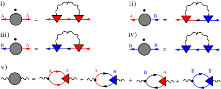
Figure 1: The truncated FRG flow equation for the fermionic self-energy in momentum transfer cutoff scheme is depicted from (i) - (iv) with $A$ and $B$ being the sublattice labels. The dot on the left-hand side represents the derivative with respect to the cutoff. The arrows illustrate the exact fermionic propagators, while the bosonic single-scale propagators are shown by slashed wavy lines. The graphical representation of the exact skeleton equation for the bosonic self-energy is shown in (v). The triangles represent the flowing three-legged vertices, while the bare ones are shown by black dots.

Finally, the FRG flow is closed by relating the vertex $\gamma_{\Lambda}$ to the wave-function renormalization factor $Z_{\Lambda}$ via the Ward identity Bauer15 ; Gonzalez10 $\gamma_{\Lambda}=1/Z_{\Lambda}$, which can be derived by comparing the FRG flow equation for $\gamma_{\Lambda}$ with the flow equation for $Z_{\Lambda}$.

We determine the cutoff-dependent quasiparticle residue, $Z_{\Lambda}$, and quasiparticle velocity, $v_{\Lambda}$, by expanding the self-energy for small frequencies and momenta,

$$\Sigma_{p}(K)=(1-Z_{\Lambda}^{-1})i\omega-(1-Y_{\Lambda}^{-1})pv_{F}\bm{\sigma}\cdot\bm{k}+\ldots,$$ (16)

so that the fermionic propagator is

$$G_{p}(K)=-Z_{\Lambda}\frac{i\omega+pv_{\Lambda}\bm{\sigma}\cdot\bm{k}}{\omega^{2}+{v}_{\Lambda}^{2}\bm{k}^{2}},$$ (17)

with renormalized quasiparticle velocity

$${v}_{\Lambda}=Z_{\Lambda}Y_{\Lambda}^{-1}v_{F}.$$ (18)

From the self-energy expression, Eq. (16), it is clear that the RG flow of $Z_{\Lambda}$ and $Y_{\Lambda}$ can be expressed in terms of the cutoff derivative of the self-energy as

$$\Lambda\partial_{\Lambda}Z_{\Lambda} = \eta_{\Lambda}Z_{\Lambda},$$ (19)

$$\Lambda\partial_{\Lambda}Y_{\Lambda} = \tilde{\eta}_{\Lambda}Y_{\Lambda},$$ (20)

with

$$\eta_{\Lambda}\ = \Lambda Z_{\Lambda}\lim_{\omega\rightarrow 0}\frac{\partial}{\partial(i\omega)}\partial_{\Lambda}\Sigma^{ss}_{p}(0,i\omega),$$ (21)

$$(\bm{\sigma}\cdot{\hat{\bm{k}}})\tilde{\eta}_{\Lambda} = -\Lambda Y_{\Lambda}\lim_{|\bm{k}|\rightarrow 0}\frac{\partial}{\partial(pv_{F}|\bm{k}|)}\partial_{\Lambda}\Sigma^{ss^{\prime}}_{p}(\bm{k},0).$$ (22)

The RG flow of the renormalized velocity ${v}_{\Lambda}=Z_{\Lambda}Y^{-1}_{\Lambda}v_{F}$ is therefore

$$\Lambda\partial_{\Lambda}{v}_{\Lambda}=({\eta}_{\Lambda}-\tilde{\eta}_{\Lambda}){v}_{\Lambda}.$$ (23)

On substituting the low-energy form of the Green’s function, Eq. (17), into the Dyson-Schwinger equation, Eq.(15), we get for the renormalized polarization

$$\Pi(Q) = \frac{N_{s}}{8}\frac{\gamma_{\Lambda}Z_{\Lambda}^{2}\bm{q}^{2}}{\sqrt{{v}_{\Lambda}^{2}\bm{q}^{2}+\bar{\omega}^{2}}}.$$ (24)

Now using the truncated FRG flow equation, Eq. (14), with corresponding renormalized fermionic propagator, Eq. (17), and renormalized polarization, Eq. (24) which is used in the bosonic single-scale propagator, we obtain

$$\eta_{\Lambda} = Z_{\Lambda}^{2}\gamma_{\Lambda}^{2}\Lambda\int_{Q}\frac{\delta(|\bm{q}|-\Lambda)}{\frac{\Lambda}{2\pi e^{2}}+\Pi(Q)}\frac{\bar{\omega}^{2}-({v}_{\Lambda}|\bm{q}|)^{2}}{[\bar{\omega}^{2}+({v}_{\Lambda}|\bm{q}|)^{2}]^{2}},$$ (25)

$$\tilde{\eta}_{\Lambda} = Z_{\Lambda}^{2}\gamma_{\Lambda}^{2}\Lambda\int_{Q}\frac{\delta(|\bm{q}|-\Lambda)}{\frac{\Lambda}{2\pi e^{2}}+\Pi(Q)}\frac{\bar{\omega}^{2}}{[\bar{\omega}^{2}+({v}_{\Lambda}|\bm{q}|)^{2}]^{2}}.$$ (26)

Note that at zero temperature these integrations can be performed exactly. Using the Ward identity, $\gamma_{\Lambda}=1/Z_{\Lambda}$, we finally obtain

$$\eta_{\Lambda} = \frac{e^{2}}{{v}_{\Lambda}}\int_{0}^{\infty}\frac{d\epsilon}{\pi}\frac{1}{u_{\Lambda}+\sqrt{1+\epsilon^{2}}}\frac{\epsilon^{2}-1}{[\epsilon^{2}+1]^{3/2}}$$ (27)

$$= \frac{e^{2}}{{v}_{\Lambda}}I_{1}(u_{\Lambda}),$$

$$\tilde{\eta}_{\Lambda} = \frac{e^{2}}{{v}_{\Lambda}}\int_{0}^{\infty}\frac{d\epsilon}{\pi}\frac{1}{u_{\Lambda}+\sqrt{1+\epsilon^{2}}}\frac{\epsilon^{2}}{[\epsilon^{2}+1]^{3/2}}$$ (28)

$$= \frac{e^{2}}{{v}_{\Lambda}}I_{2}(u_{\Lambda}),$$

where we have introduced the dimensionless coupling

$$u_{\Lambda}=Z_{\Lambda}^{2}\gamma_{\Lambda}\frac{N_{s}}{8}\frac{2\pi e^{2}}{{v}_{\Lambda}}=\pi N_{s}Y_{\Lambda}\frac{\alpha}{4}.$$ (29)

Thus, we obtain a closed system of flow equations for $Z_{\Lambda}$ and $v_{\Lambda}$. On introducing the logarithmic flow parameter $l=\ln(\Lambda_{0}/\Lambda)$, the dimensionless velocity $\tilde{v}_{l}=v_{\Lambda}/v_{F}$, and on writing $Z_{l}=Z_{\Lambda_{0}e^{-l}}$, we finally obtain

$$\partial_{l}Z_{l} = -\alpha\frac{Z_{l}}{\tilde{v}_{l}}I_{1}\left(c\frac{Z_{l}}{\tilde{v}_{l}}\right),$$ (30)

$$\partial_{l}\tilde{v}_{l} = \alpha\left[I_{2}\left(c\frac{Z_{l}}{\tilde{v}_{l}}\right)-I_{1}\left(c\frac{Z_{l}}{\tilde{v}_{l}}\right)\right],$$ (31)

where

$$c=\frac{\pi N_{s}\alpha}{4}=\frac{\pi\alpha}{2}$$ (32)

and the integrals $I_{1}(u)$ as well as $I_{2}(u)$, as given in Eqs.(27) and (28), can be performed analytically. For $u\leq 1$, they are given by

$$I_{1}(u) = \frac{1}{\pi u^{2}}\left[\pi-2u-\frac{2-u^{2}}{\sqrt{1-u^{2}}}\arctan\left(\frac{\sqrt{1-u^{2}}}{u}\right)\right],$$

$$I_{2}(u) = \frac{1}{\pi u^{2}}\left[\frac{\pi}{2}-u-\sqrt{1-u^{2}}\arctan\left(\frac{\sqrt{1-u^{2}}}{u}\right)\right],$$

while for $u>1$ they become

$$I_{1}(u) = \frac{1}{\pi u^{2}}\left[\pi-2u-\frac{2-u^{2}}{2\sqrt{u^{2}-1}}\ln\left(\frac{u+\sqrt{u^{2}-1}}{u-\sqrt{u^{2}-1}}\right)\right],$$

$$I_{2}(u) = \frac{1}{\pi u^{2}}\left[\frac{\pi}{2}-u+\frac{\sqrt{u^{2}-1}}{2}\ln\left(\frac{u+\sqrt{u^{2}-1}}{u-\sqrt{u^{2}-1}}\right)\right].$$

For $u\ll 1$ the integrals can be approximated by

$$I_{1}(u) = \frac{u}{3\pi}-\frac{u^{2}}{8}+{\cal{O}}(u^{3}),$$ (37)

$$I_{2}(u) = \frac{1}{4}-\frac{u}{3\pi}+\frac{u^{2}}{16}+{\cal{O}}(u^{3}).$$ (38)

III Results

III.1 Static screening approximation

Before presenting the numerical solution of Eqs. (30) and (31), it is instructive to consider the corresponding RG flow in the approximation where the frequency dependence of the polarization is neglected. Approximating $\Pi(i\bar{\omega},\bm{q})\approx\Pi(0,\bm{q})$ in Eq. (24), the integral for $\tilde{\eta}_{\Lambda}$ in Eq. (28) simplifies to

$$\tilde{\eta}_{\Lambda}=\frac{e^{2}}{4}\frac{1}{v_{\Lambda}+cv_{F}}.$$ (39)

The flow of the dimensionless velocity $\tilde{v}_{l}=v_{\Lambda}/v_{F}$, in this approximation, is determined by

$$\partial_{l}\tilde{v}_{l}=\frac{b}{1+c/\tilde{v}_{l}},$$ (40)

where we have defined

$$b=\alpha I_{2}(0)=\frac{\alpha}{4}=\frac{e^{2}}{4v_{F}}.$$ (41)

The solution of the differential equation (40) with initial condition $\tilde{v}_{0}=1$ is given by the solution of the implicit equation,

$$\tilde{v}_{l}+c\ln\tilde{v}_{l}=1+bl,$$ (42)

which can be expressed in terms of the so-called Lambert $W$-function Corless96 $W(x)$ (also called product logarithm),

$$\tilde{v}_{l}=cW\left(\frac{e^{(1+bl)/c}}{c}\right)=cW\left[\frac{e^{1/c}}{c}\left(\frac{\Lambda_{0}}{\Lambda}\right)^{\frac{b}{c}}\right].$$ (43)

We use the fact that by definition the Lambert $W$-function is the solution of $We^{W}=x$ and hence $W(x)=\ln[x/W(x)]$. Therefore, we may alternatively write the solution of the differential equation (40) as,

$$\tilde{v}_{l} = c\ln\left[\frac{e^{(1+bl)/c}}{cW\left(\frac{e^{(1+bl)/c}}{c}\right)}\right]$$ (44)

$$= 1+bl-c\ln\left[cW\left(\frac{e^{(1+bl)/c}}{c}\right)\right].$$

Using the fact that $cW(e^{1/c}/c)=1$, we immediately see that our solution indeed satisfies the initial condition $\tilde{v}_{l=0}=1$. Finally, in order to obtain the momentum dependence of the quasiparticle velocity, we identify that $v(k)=v_{\Lambda=k}$. Recently, we have explicitly confirmed the validity of this identification using the FRG method Bauer15 . Physically this procedure is based on the fact that for $\Lambda\ll k$ the external momentum $k$ acts as an infrared cutoff. Therefore, we obtain $B(\alpha)=\alpha/4$ as the prefactor of the logarithm in Eq. (5). We substitute $l=\ln(\Lambda_{0}/\Lambda)$ and obtain for the cutoff-dependent velocity,

$$\frac{v_{\Lambda}}{v_{F}}=1+\frac{\alpha}{4}\ln\left(\frac{C_{\Lambda}(\alpha)}{\Lambda}\right),$$ (45)

with scale- and interaction-dependent cutoff

$$C_{\Lambda}(\alpha)=\frac{\Lambda_{0}}{\left\{cW\left[\frac{e^{1/c}}{c}\left(\frac{\Lambda_{0}}{\Lambda}\right)^{b/c}\right]\right\}^{c/b}}.$$ (46)

For large $x$ the Lambert $W$-function can be approximated by

$$W(x)\approx\ln x-\ln\ln x+\frac{\ln\ln x}{\ln x}.$$ (47)

We retain only the first term of the large $x$ asymptotic expansion as well as using $c/b=\pi N_{s}$; we obtain for $\Lambda\rightarrow 0$,

$$C_{\Lambda}(\alpha)\approx\frac{\Lambda_{0}}{\left[1-c\ln c+\frac{\alpha}{4}\ln(\Lambda_{0}/\Lambda)\right]^{\pi N_{s}}}.$$ (48)

On substituting this approximation into Eq. (45) and formally expanding the result for small $\alpha$, we obtain

$$v_{\Lambda}/v_{F} = F_{0}(\alpha)+F_{1}(\alpha)\ln(\Lambda_{0}/\Lambda)+F_{2}(\alpha)\ln^{2}(\Lambda_{0}/\Lambda)$$ (49)

$$+{\cal{O}}[\alpha^{4}\ln^{3}(\Lambda_{0}/\Lambda)],$$

with interaction-dependent coefficients

$$F_{0}(\alpha) = 1+\frac{(\pi N_{s})^{2}}{16}\alpha^{2}\ln\left(\frac{\pi N_{s}}{4}\alpha\right)$$ (50a)

$$+ \frac{(\pi N_{s})^{2}}{128}\alpha^{3}\ln^{2}\left(\frac{\pi N_{s}}{4}\alpha\right)+{\cal{O}}(\alpha^{4}),$$

$$F_{1}(\alpha) = \frac{\alpha}{4}-\frac{\pi N_{s}}{16}\alpha^{2}$$ (50b)

$$- \frac{(\pi N_{s})^{2}}{64}\alpha^{3}\ln\left(\frac{\pi N_{s}}{4}\alpha\right)+{\cal{O}}(\alpha^{4}),$$

$$F_{2}(\alpha) = \frac{\pi N_{s}}{128}\alpha^{3}+{\cal{O}}(\alpha^{4}).$$ (50c)

Comparing the above results with the perturbative expansions, as given in Eqs. (3) and (4), and setting now explicitly $N_{s}=2$, we conclude that, within our truncation scheme, the first two coefficients in the expansion of $F_{1}(\alpha)$ are given by

$$f_{1}^{(1)}=\frac{1}{4},\;\;\;f_{1}^{(2)}=-\frac{\pi}{8}\approx-0.39,$$ (51)

while the coefficient of the leading $\alpha^{3}$ term in the weak-coupling expansion of $F_{2}(\alpha)$ is

$$f_{2}^{(3)}=\frac{\pi}{64}\approx 0.049.$$ (52)

Keeping in mind that the coefficient $F_{0}(\alpha)$ can be normalized to unity by redefining the ultraviolet cutoff, we conclude that the above structure of the perturbation series is equivalent with the series in Eq. (2) previously derived by Barnes et al. [Barnes14, ].

We note that according to Mishchenko Mishchenko07 the numerical value of the two-loop coefficient is $f_{1}^{(2)}=-\frac{5}{6}+\ln 2\approx-0.140$. On the other hand, Vafek and Case Vafek08 found $f_{1}^{(2)}=-\frac{1}{3}+\frac{103}{96}-\frac{3}{2}\ln 2\approx-0.300$, while Sharma et al. Sharma12 obtained $f_{1}^{(2)}=-\frac{1}{3}$, and more recently Barnes et al. Barnes14 got $f_{1}^{(2)}=-\frac{2}{3}+\frac{1}{2}\ln 2\approx-0.320$. Given the simplicity of our truncation, our result for the two-loop coefficient $f_{1}^{(2)}\approx-0.39$ is reasonably close to the results of aforementioned calculations Mishchenko07 ; Vafek08 ; Sharma12 ; Barnes14 . Note that recently Barnes et al. Barnes14 found that the three-loop coefficient $f_{2}^{(3)}$ is minus one-eighth of the two-loop coefficient $f_{1}^{(2)}$, which is confirmed by our calculation. Although the static screening approximation is not expected to give a quantitatively accurate result, the fact that the perturbative expansion of the renormalized velocity, Eq. (45), in powers of $\alpha$ reproduces the known structure of perturbation theory Barnes14 gives us confidence that our RG approach indeed resums the entire perturbation series in a sensible way.

III.2 Including dynamic screening

We now present our results obtained from the numerical solution of Eqs. (30) and (31) which take the frequency dependence of the polarization into account. In Fig. 2 we show the RG flow of $\tilde{v}_{l}$ as a function of the logarithmic flow parameter $l=\ln(\Lambda_{0}/\Lambda)$ for the physically relevant value $\alpha=2.2$. For comparison, we also show our analytical result (45) in static screening approximation and the perturbative one-loop RG result $\tilde{v}_{l}=1+(\alpha/4)l$.

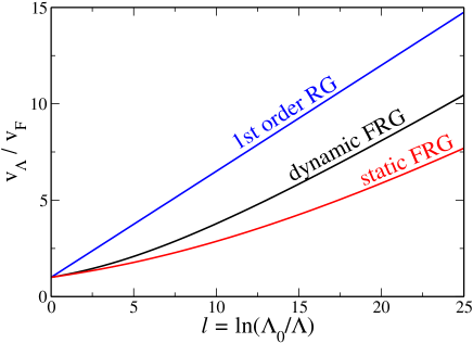
Figure 2: The RG flow of the dimensionless velocity $\tilde{v}_{l}=v_{\Lambda}/v_{F}$ (black middle line), as obtained from the numerical solution of Eqs. (30) and (31), is shown as a function of the flow parameter $l=\ln(\Lambda_{0}/\Lambda)$ for $\alpha=2.2$. The corresponding result (45) in static screening approximation (lower red line), and the perturbative one-loop RG result $\tilde{v}_{l}=1+(\alpha/4)l$ (upper blue line) are also presented.

The corresponding RG flow of the quasiparticle residue is shown in Fig. 3. It is apparent that for $l\rightarrow\infty$ the quasiparticle residue approaches a finite constant,

$$Z_{\ast}=\lim_{l\rightarrow\infty}Z_{l}\approx 0.4772,$$ (53)

while the quasiparticle velocity diverges.

Figure 3: The RG flow of quasiparticle residue $Z_{\Lambda}$ (solid line), as obtained from the numerical solution of Eqs. (30) and (31), is shown as a function of the flow parameter $l=\ln(\Lambda_{0}/\Lambda)$ for $\alpha=2.2$. The dashed line represents $Z_{\ast}=\lim_{l\rightarrow\infty}Z_{l}\approx 0.4772$.

To quantify this divergence, let us assume that the functional form (45) obtained in static screening approximation remains qualitatively correct so that the cutoff-dependent velocity is of the form

$$\frac{v_{\Lambda}}{v_{F}}=1+B(\alpha)\ln\left(\frac{C_{\Lambda}(\alpha)}{\Lambda}\right),$$ (54)

which can be obtained from $v(k)$ in Eq. (5) by substituting $k\rightarrow\Lambda$. Anticipating that the cutoff function $C_{\Lambda}(\alpha)$ vanishes logarithmically for $\Lambda\rightarrow 0$, as seen in the static screening approximation, we may identify

$$B(\alpha) = \lim_{l\rightarrow\infty}\partial_{l}\tilde{v}_{l}$$ (55)

$$= \alpha\lim_{l\rightarrow\infty}\left[I_{2}\left(cZ_{l}/\tilde{v}_{l}\right)-I_{1}\left(cZ_{l}/\tilde{v}_{l}\right)\right].$$

But we already know that $Z_{l}$ approaches a finite limit while $\tilde{v}_{l}$ diverges for $l\rightarrow\infty$, so within our truncation we obtain

$$B(\alpha)=\alpha I_{2}(0)=\frac{\alpha}{4}.$$ (56)

The frequency dependence of the polarization therefore does not modify the form (45) of the cutoff dependent velocity. From the numerical solution $\tilde{v}_{l}$ of the flow equation (31), the cutoff function $C_{\Lambda}(\alpha)$ in Eq. (54) can be obtained as

$$C_{\Lambda}(\alpha)=\Lambda e^{4(\tilde{v}_{l}-1)/\alpha}.$$ (57)

On inserting the perturbative one-loop result $\tilde{v}_{l}-1=(\alpha/4)l=(\alpha/4)\ln(\Lambda_{0}/\Lambda)$, we obtain $C_{\Lambda}(\alpha)=\Lambda_{0}$. However, if we substitute for $\tilde{v}_{l}$ the solution of Eqs. (30) and (31) we find that for any finite $\alpha$ the function $C_{\Lambda}(\alpha)$ vanishes for $\Lambda\rightarrow 0$, as shown in Fig. 4.

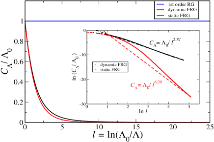
Figure 4: Cutoff $C_{\Lambda}(\alpha)$ as a function of the logarithmic flow parameter $l=\ln(\Lambda_{0}/\Lambda)$ for $\alpha=2.2$. The black solid line is obtained by inserting the solution of the flow equations (30) and (31) into $C_{\Lambda}(\alpha)=\Lambda e^{4(\tilde{v}_{l}-1)/\alpha}$. The red solid line is the corresponding function in static screening approximation given in Eq. (46), while the horizontal blue solid line is the perturbative one-loop result $C_{\Lambda}=\Lambda_{0}$. The double-logarithmic plot in the inset shows $\ln(C_{\Lambda}/\Lambda_{0})$ versus $\ln l=\ln\ln(\Lambda_{0}/\Lambda)$. The black dashed line is a fit of the asymptotics for large $\ln l$ given by the straight line $\ln(C_{\Lambda}/\Lambda_{0})=-2.81\ln l$. The red dashed line is the known asymptotics in static screening approximation, which according to Eq. (48) gives $\ln(C_{\Lambda}/\Lambda_{0})\sim-2\pi\ln l$.

For comparison, we also show the result (46) of the static screening approximation. In order to quantify the modifications due to dynamic screening, we present in the inset of Fig. 4 a double-logarithmic plot of $\ln[C_{\Lambda}/\Lambda_{0}]$ versus $\ln l=\ln\ln(\Lambda_{0}/\Lambda)$. From the slope of the asymptotic straight line, for large $\ln l$, we see that,

$$\frac{C_{\Lambda}}{\Lambda_{0}}\sim\frac{c_{1}}{[\ln(\frac{\Lambda_{0}}{\Lambda})]^{x}},$$ (58)

with $x\approx 2.81$ and $c_{1}$ being a numerical constant of order unity. Note that in static screening approximation we found $x=\pi N_{s}=2\pi$, Eq. (48), so that dynamic screening modifies the power of the logarithmic decay of the cutoff $C_{\Lambda}$ for $\Lambda\rightarrow 0$.

IV Summary and outlook

With a strong motivation to resolve the puzzle related to interaction effects in graphene, we have reconsidered the problem of calculating the renormalized quasiparticle velocity for momenta close to the Dirac points in undoped graphene. On combining a FRG flow equation for the fermionic self-energy with a Dyson-Schwinger equation for the particle-hole bubble and a Ward identity for the three-legged (Yukawa) vertex, we have derived and solved a closed system of RG flow equations for the quasiparticle velocity and the quasiparticle residue. In contrast to the fermionic cutoff scheme Bauer15 , we have introduced a cutoff only in the bosonic Hubbard-Stratonovich field which mediates the interaction in the forward scattering channel. An important advantage of this momentum transfer cutoff scheme Schuetz05 is that, in the static limit, the flow equation for the renormalized velocity can be solved exactly and the asymptotic behavior of the velocity can be extracted analytically.
Our main result is that the cutoff scale below which the logarithmic singularity of the quasiparticle velocity becomes apparent is itself logarithmically suppressed. In static screening approximation, we expand our RG result in powers of the bare coupling $\alpha$ and reconcile with the peculiar structure of the perturbative expansion of $v(k)$ in powers of $\alpha$ as found by Barnes et al. Barnes14 . Although the higher-order logarithmic corrections become dominant only in the close vicinity of the Dirac points, which probably cannot be resolved experimentally, it is conceptually important to highlight the character of the multilogarithmic singularity of the renormalized velocity and thus unfolding the nature of interaction effects in graphene.

As an outlook, our approach might also be useful in determining the critical interaction strength related to chiral symmetry breaking in graphene Drut09 . Recently, this problem was studied by Katanin  Katanin16 using a purely fermionic FRG approach who found that vertex corrections are crucially important to obtain an accurate estimate of the critical interaction strength in graphene.

References

• (1) A. K. Geim and K. S. Novoselov, Nat. Mater. 6, 183 (2007).
• (2) A. H. Castro Neto, F. Guinea, N. M. R. Peres, K. S. Novoselov, and A. K. Geim, Rev. Mod. Phys. 81, 109 (2009).
• (3) S. Das Sarma, S. Adam, E. H. Hwang, and E. Rossi, Rev. Mod. Phys. 83, 407 (2011).
• (4) F. Schwierz, Nat. Nanotechnol. 5, 487 (2010).
• (5) F. Bonaccorso, Z. Sun, T. Hasan, and A. C. Ferrari, Nat. Photonics 4, 611 (2010).
• (6) P. Avouris, Nano Lett. 10, 4285 (2010).
• (7) V. N. Kotov, B. Uchoa, V. M. Pereira, F. Guinea, and A. H. Castro Neto, Rev. Mod. Phys. 84, 1067 (2012).
• (8) J. González, F. Guinea, and M. A. H. Vozmediano, Nucl. Phys. B 424, 595 (1994).
• (9) J. González, F. Guinea, and M. A. H. Vozmediano, Phys. Rev. B 59, R2474 (1999).
• (10) I. F. Herbut, Phys. Rev. Lett. 97, 146401 (2006).
• (11) A. Bostwick, T. Ohta, T. Seyller, K. Horn, and E. Rotenberg, Nat. Phys. 3, 36 (2007).
• (12) S. Das Sarma, E. H. Hwang, and W.-K. Tse, Phys. Rev. B 75, 121406(R) (2007).
• (13) K. S. Novoselov, Z. Jiang, Y. Zhang, S. V. Morozov, H. L. Stormer, U. Zeitler, J. C. Maan, G. S. Boebinger, P. Kim, and A. K. Geim, Science 315, 1379 (2007).
• (14) E. G. Mishchenko, Phys. Rev. Lett. 98, 216801 (2007).
• (15) O. Vafek, Phys. Rev. Lett. 98, 216401 (2007).
• (16) D. T. Son, Phys. Rev. B 75, 235423 (2007).
• (17) O. Vafek and M. J. Case, Phys. Rev. B 77, 033410 (2008).
• (18) I. F. Herbut, V. Juričić, and O. Vafek, Phys. Rev. Lett. 100, 046403 (2008).
• (19) J. E. Drut and D. T. Son, Phys. Rev. B 77, 075115 (2008).
• (20) M. S. Foster and I. L. Aleiner, Phys. Rev. B 77, 195413 (2008).
• (21) V. N. Kotov, B. Uchoa, and A. H. Castro Neto, Phys. Rev. B 78, 035119 (2008).
• (22) D. C. Elias, R. V. Gorbachev, A. S. Mayorov, S. V. Morozov, A. A. Zhukov, P. Blake, L. A. Ponomarenko, I. V. Grigorieva, K. S. Novoselov, F. Guinea, and A. K. Geim, Nat. Phys. 7, 701 (2011).
• (23) A. Sharma, V. N. Kotov, and A. H. Castro Neto, arXiv:1206.5427 (2012).
• (24) J. Chae, S. Jung, A. F. Young, C. R. Dean, L. Wang, Y. Gao, K. Watanabe, T. Taniguchi, J. Hone, K. L. Shepard, P. Kim, N. B. Zhitenev, and J. A. Stroscio, Phys. Rev. Lett. 109, 116802 (2012).
• (25) E. Barnes, E. H. Hwang, R. E. Throckmorton, and S. Das Sarma, Phys. Rev. B 89, 235431 (2014).
• (26) J. Hofmann, E. Barnes, and S. Das Sarma, Phys. Rev. Lett. 113, 105502 (2014).
• (27) C. Bauer, A. Rückriegel, A. Sharma, and P. Kopietz, Phys. Rev. B 92, 121409(R) (2015).
• (28) C. Hwang, D. A. Siegel, S.-K. Mo, W. Regan, A. Ismach, Y. Zhang, A. Zettl, and A. Lanzara, Sci. Rep. 2, 590 (2012).
• (29) P. Kopietz, L. Bartosch, and F. Schütz, Introduction to the Functional Renormalization Group (Springer, Berlin, 2010).
• (30) W. Metzner, M. Salmhofer, C. Honerkamp, V. Meden, and K. Schönhammer, Rev. Mod. Phys. 84, 299 (2012).
• (31) F. Schütz, L. Bartosch, and P. Kopietz, Phys. Rev. B 72, 035107 (2005).
• (32) F. Schütz and P. Kopietz, J. Phys. A: Math. Gen. 39, 8205 (2006).
• (33) C. Drukier, L. Bartosch, A. Isidori, and P. Kopietz, Phys. Rev. B 85, 245120 (2012).
• (34) J. González, Phys. Rev. B 82, 155404 (2010).
• (35) R. M. Corless, G. H. Gonnet, D. E. G. Hare, D. J. Jeffrey, and D. E. Knuth, Adv. Comput. Math. 5, 329 (1996).
• (36) J. E. Drut and T. A. Lähde, Phys. Rev. Lett. 102, 026802 (2009).
• (37) A. Katanin, Phys. Rev. B 93, 035132 (2016).