Invariant domains preserving ALE
approximation of hyperbolic systems with
continuous finite elements

Abstract

A conservative invariant domain preserving Arbitrary Lagrangian Eulerian method for solving nonlinear hyperbolic systems is introduced. The method is explicit in time, works with continuous finite elements and is first-order accurate in space. One originality of the present work is that the artificial viscosity is unambiguously defined irrespective of the mesh geometry/anisotropy and does not depend on any ad hoc parameter. The proposed method is meant to be a stepping stone for the construction of higher-order methods in space by using appropriate limitation techniques.

1 Introduction

Consider the following hyperbolic system in conservative form

(1) $$\begin{cases}\partial_{t}{\bm{u}}+\nabla{\cdot}{\bm{f}}({\bm{u}})=0,\quad\mbox{for}\,({\bm{x}},t)\in{\mathbb{R}}^{d}{\times}{\mathbb{R}}_{+}.\\ {\bm{u}}({\bm{x}},0)={\bm{u}}_{0}({\bm{x}}),\quad\mbox{for}\,{\bm{x}}\in{\mathbb{R}}^{d},\end{cases}$$

where the dependent variable ${\bm{u}}$ is ${\mathbb{R}}^{m}$-valued and the flux ${\bm{f}}$ is ${\mathbb{R}}^{m{\times}d}$-valued. The objective of this paper is to investigate an approximation technique for solving (1) using an Arbitrary Lagrangian Eulerian (ALE) formulation with continuous finite elements and explicit time stepping on non-uniform meshes in any space dimension.

The interest for finite elements in the context of compressible Lagrangian hydrodynamics has been recently revived by the work of Dobrev et al. [13], where the authors have demonstrated that high-order finite elements have good properties in terms of geometry representation, symmetry preservation, resolution of shock fronts and high-order convergence rate for smooth solutions. The finite element formalism has been combined with staggered grid hydrodynamics methods in Barlow [3], Scovazzi et al. [32] and with cell-centered hydrodynamics methods in Vilar et al. [35] in the form of a Discontinuous Galerkin scheme. One common factor of all these papers is that the stabilization is done by introducing some artificial viscosity to control post-shock oscillations, and high-order convergence in space is achieved by restricting the diffusion to be active only in the singular regions of the solution. This can be done in many ways, for instance by measuring smoothness like in the ENO/WENO literature like in Cheng and Shu [10] or by using entropies like in the entropy viscosity methodology of Guermond et al. [21]. A detailed list of requirements and specific artificial viscosity expressions for Lagrangian hydrodynamics have been proposed by Caramana et al. [6], Caramana and Loubère [7], Shashkov and Campbell [33], Kolev and Rieben [25], Lipnikov and Shashkov [30]. The artificial viscosity can also be implicitly introduced by using Godunov type or cell-centered type methods based on Riemann solvers, see e.g., Boscheri and Dumbser [4], Carré et al. [8].

In the present paper we revisit the artificial viscosity problem for general hyperbolic systems like (1) using an Arbitrary Lagrangian Eulerian (ALE) formulation and explicit time stepping. The originality of the present work is that (i) The approximation in space is done with continuous finite elements of arbitrary order; (ii) The local shape functions can be linear Lagrange elements, Bernstein-Bezier elements of any order or any other nonnegative functions (not necessarily polynomials) that have the partition of unity property; (iii) The finite element meshes considered are non-uniform, curvilinear and the space dimension is arbitrary; (iv) The artificial viscosity is unambiguously defined irrespective of the mesh geometry/anisotropy, does not depend on any ad hoc parameter, contrary to what has been previously done in the finite element literature, and leads to precise invariant domain properties and entropy inequalities; (v) The methods works for any (reasonable in the sense of §2) hyperbolic system. Although entirely based on continuous finite elements, our work is deeply rooted in the work of Lax [28] and Hoff [24], and in some sense mimics well established schemes from the finite volume literature, e.g., Guillard and Farhat [22], Farhat et al. [14] or the discontinuous Galerkin literature, e.g., Vilar et al. [35]. The proposed method is meant to be a stepping stone for the construction of higher-order methods in space by using, for instance, the flux transport correction methodology à la Boris-Book-Zalesak, or any generalization thereof, to implement limitation. None of these generalizations are discussed in the paper. The sole objective of the present work is to give a firm, undisputable, theoretical footing to the first-order, invariant-domain preserving, method.

The paper is organized as follows. We introduce some notation and recall important properties about the one-dimensional Riemann problem in §2. We introduce notation relative to mesh motion and Lagrangian mappings in §3. The results established in §2 and §3 are standard and will be invoked in §4 and §5. The reader who is familiar with these notions is invited to go directly to §4. We describe in §4 two versions of an ALE algorithm to approximate the solution of (1). The first algorithm, henceforth referred to as version 1, is composed of the steps (22)-(23)-(24)-(28). The second algorithm, i.e., version 2, is composed of the steps (45)-(46)-(47)-(48)-(28). The key difference between these two algorithms is the way the mass carried by the shape functions is updated (compare (23) and (47)). Only version 1 can be easily made high-order in time by means of the strong stability preserving technology (see Ferracina and Spijker [15], Higueras [23], Gottlieb et al. [18] for details on SSP techniques). It is proved in §5 that under the appropriate CFL condition both algorithms are invariant domain preserving, conservative and satisfy a local entropy inequality for any admissible entropy pair. The main results of this section are Theorem 5.28 and Theorem 5.37. The SSP RK3 extension of scheme 1 is tested numerically in §6 on scalar conservation equations and on the compressible Euler equations using two different finite element implementations of the method. In all the cases the ALE velocity is ad hoc and no particular effort has been made to optimize this quantity. The purpose of this paper is not to design an optimal ALE velocity but to propose an algorithm that is conservative and invariant domain preserving for any reasonable ALE velocity.

2 Riemann problem and invariant domain

We recall in this section elementary properties of Riemann problems that will be used in the paper.

2.1 Notation and boundary conditions

In this paper the dependent variable ${\bm{u}}$ in (1) is considered as a column vector ${\bm{u}}=(u_{1},\ldots,u_{m})^{\mathsf{T}}$. The flux is a matrix with entries $f_{ij}({\bm{u}})$, $1\leq i\leq m$, $1\leq j\leq d$. We denote ${\bm{f}}_{i}$ the row vector $(f_{i1},\ldots,f_{id})$, $i\in\{1\hskip 0.50003pt{:}\hskip 1.00006ptm\}$. We denote by $\nabla{\cdot}{\bm{f}}$ the column vector with entries $(\nabla{\cdot}{\bm{f}})_{i}=\sum_{1\leq j\leq d}\partial_{x_{j}}f_{ij}$. For any ${\bm{n}}=(n_{1}\ldots,n_{d})^{\mathsf{T}}\in{\mathbb{R}}^{d}$, we denote ${\bm{f}}({\bm{u}}){\cdot}{\bm{n}}$ the column vector with entries ${\bm{f}}_{i}({\bm{u}}){\cdot}{\bm{n}}=\sum_{1\leq l\leq d}n_{l}f_{il}({\bm{u}})$, where $i\in\{1\hskip 0.50003pt{:}\hskip 1.00006ptm\}$. Given two vector fields, say ${\bm{u}}\in{\mathbb{R}}^{m}$ and ${\bm{v}}\in{\mathbb{R}}^{d}$, we define ${\bm{u}}\otimes{\bm{v}}$ to be the $m{\times}d$ matrix with entries $u_{i}v_{j}$, $i\in\{1\hskip 0.50003pt{:}\hskip 1.00006ptm\}$, $j\in\{1\hskip 0.50003pt{:}\hskip 1.00006ptd\}$. We also define $\nabla{\cdot}({\bm{u}}\otimes{\bm{v}})$ to be the column vector with entries $\nabla{\cdot}({\bm{u}}\otimes{\bm{v}})_{i}=\sum_{j=1}^{d}\partial_{j}(u_{i}v_{j})$. The unit sphere in ${\mathbb{R}}^{d}$ centered at $0$ is denoted by $S^{d-1}({\bm{0}},1)$.

To simplify questions regarding boundary conditions, we assume that the initial data is constant outside a compact set and we solve the Cauchy problem in ${\mathbb{R}}^{d}$ or we use periodic boundary conditions.

2.2 One-dimensional Riemann problem

We are not going to try to define weak solutions to (1), but instead we assume that there is a clear notion for the solution of the Riemann problem. To stay general we introduce a generic hyperbolic flux ${\bm{h}}$ and we say that $(\eta,{\bm{q}})$ is an entropy pair associated with the flux ${\bm{h}}$ if $\eta$ is convex and the following identity holds:

(2) $$\partial_{v_{k}}({\bm{q}}({\bm{v}}){\cdot}{\bm{n}})=\sum_{i=1}^{m}\partial_{v_{i}}\eta({\bm{v}})\partial_{v_{k}}({\bm{h}}_{i}({\bm{v}}){\cdot}{\bm{n}}),\qquad\forall k\in\{1\hskip 0.50003pt{:}\hskip 1.00006ptm\},\ \forall{\bm{n}}\in S^{d-1}({\bm{0}},1).$$

We refer to Chen [9, §2] for more details on convex entropies and symmetrization. In the rest of the paper we assume that there exists a nonempty admissible set ${\mathcal{A}}_{\bm{h}}\subset{\mathbb{R}}^{m}$ such that the following one-dimensional Riemann problem

(3) $$\partial_{t}{\bm{u}}+\partial_{x}({\bm{h}}({\bm{u}}){\cdot}{\bm{n}})=0,\quad(x,t)\in{\mathbb{R}}{\times}{\mathbb{R}}_{+},\qquad{\bm{u}}(x,0)=\begin{cases}{\bm{u}}_{L},&\text{if $x<0$}\\ {\bm{u}}_{R},&\text{if $x>0$},\end{cases}$$

has a unique entropy satisfying solution for any pair of states $({\bm{u}}_{L},{\bm{u}}_{R})\in{\mathcal{A}}_{\bm{h}}{\times}{\mathcal{A}}_{\bm{h}}$ and any unit vector ${\bm{n}}\in S^{d-1}({\bm{0}},1)$. We henceforth denote the solution to this problem by ${\bm{u}}({\bm{h}},{\bm{n}},{\bm{u}}_{L},{\bm{u}}_{R})$. We also say that ${\bm{u}}$ is an entropy satisfying solution of (3) if the following holds in the distribution sense

(4) $$\partial_{t}\eta({\bm{u}})+\partial_{x}({\bm{q}}({\bm{u}}){\cdot}{\bm{n}})\leq 0.$$

for any entropy pair $(\eta,{\bm{q}})$.

It is unrealistic to expect a general theory of the Riemann problem (3) for arbitrary nonlinear hyperbolic systems with large data, we henceforth make the following assumption:

(5) $$\begin{aligned} &\text{The unique solution of \eqref{def:Riemann_problem} has a finite speed of}\\[-3.0pt] &\text{propagation for any ${\bm{n}}$ and any $({\bm{u}}_{L},{\bm{u}}_{R})\in{\mathcal{A}}_{\bm{h}}{\times}{\mathcal{A}}_{\bm{h}}$, i.e.,\@}\\[-3.0pt] &\text{there are $\lambda_{L}({\bm{h}},{\bm{n}},{\bm{u}}_{L},{\bm{u}}_{R})\leq\lambda_{R}({\bm{h}},{\bm{n}},{\bm{u}}_{L},{\bm{u}}_{R})$ such}\\ &{\bm{u}}(x,t)=\begin{cases}{\bm{u}}_{L},&\text{if $x\leq t\lambda_{L}({\bm{h}},{\bm{n}},{\bm{u}}_{L},{\bm{u}}_{R})$}\\ {\bm{u}}_{R},&\text{if $x\geq t\lambda_{R}({\bm{h}},{\bm{n}},{\bm{u}}_{L},{\bm{u}}_{R})$}.\end{cases}\end{aligned}$$

This assumption is known to hold for small data when the system is strictly hyperbolic with smooth flux and all the characteristic fields are either genuinely nonlinear or linearly degenerate. More precisely there exists $\delta>0$ such that the Riemann problem has a unique self-similar weak solution in Lax’s form for any initial data such that $\|{\bm{u}}_{L}-{\bm{u}}_{R}\|_{\ell^{2}}\leq\delta$, see Lax [29] and Bressan [5, Thm 5.3]. In particular there are $2m$ numbers $\lambda_{1}^{-}\leq\lambda_{1}^{+}\leq\lambda_{2}^{-}\leq\lambda_{2}^{+}\leq\ldots\leq\lambda_{m}^{-}\leq\lambda_{m}^{+}$, defining up to $2m+1$ sectors (some could be empty) in the $(x,t)$ plane:

(6) $$\frac{x}{t}\in(-\infty,\lambda_{1}^{-}),\quad\frac{x}{t}\in(\lambda_{1}^{-},\lambda_{1}^{+}),\ldots,\quad\frac{x}{t}\in(\lambda_{m}^{-},\lambda_{m}^{+}),\quad\frac{x}{t}\in(\lambda_{m}^{+},\infty).$$

where the Riemann solution is ${\bm{u}}_{L}$ in the sector $\frac{x}{t}\in(-\infty,\lambda_{1}^{-})$, ${\bm{u}}_{R}$ in the last sector $\frac{x}{t}\in(\lambda_{m}^{+},\infty)$, and either a constant state or an expansion in the other sectors, see [5, Chap. 5]. In this case we have $\lambda_{L}:=\lambda_{L}({\bm{h}},{\bm{n}},{\bm{u}}_{L},{\bm{u}}_{R})=\lambda_{1}^{-}$ and $\lambda_{R}:=\lambda_{R}({\bm{h}},{\bm{n}},{\bm{u}}_{L},{\bm{u}}_{R})=\lambda_{m}^{+}$. The sector $\lambda_{1}^{-}t<x<\lambda_{m}^{+}t$, $0<t$, is henceforth referred to as the Riemann fan. The maximum wave speed in the Riemann fan is $\lambda_{\max}:=\lambda_{\max}({\bm{h}},{\bm{n}},{\bm{u}}_{L},{\bm{u}}_{R}):=\max(|\lambda_{L}|,|\lambda_{R}|)$. For brevity, when there is no ambiguity, we will omit the dependence of $\lambda_{L},\lambda_{R}$ and $\lambda_{\max}$ on the parameters ${\bm{h}},{\bm{n}},{\bm{u}}_{L},{\bm{u}}_{R}$. The finite speed assumption (5) holds in the case of strictly hyperbolic systems that may have characteristic families that are either not genuinely nonlinear or not linearly degenerate, see e.g., Dafermos [12, Thm. 9.5.1].

2.3 Invariant sets and domains

The following elementary result is an important, well-known, consequence of the Riemann fan assumption (5):

Lemma 1.

Let ${\bm{h}}$ be a hyperbolic flux over the admissible set ${\mathcal{A}}_{\bm{h}}$ and satisfying the finite wave speed assumption (5). Let ${\bm{v}}({\bm{h}},{\bm{n}},{\bm{v}}_{L},{\bm{v}}_{R})$ be the unique solution to the problem $\partial_{t}{\bm{v}}+\partial_{x}({\bm{h}}({\bm{v}}){\cdot}{\bm{n}})=0$ with initial data ${\bm{v}}_{L},{\bm{v}}_{R}\in{\mathcal{A}}_{\bm{h}}$. Let $(\eta,{\bm{q}})$ be an entropy pair associated with the flux ${\bm{h}}$. Assume that $t\,\lambda_{\max}({\bm{h}},{\bm{n}},{\bm{v}}_{L},{\bm{v}}_{R})\leq\frac{1}{2}$ and let $\overline{\bm{v}}(t,{\bm{h}},{\bm{n}},{\bm{v}}_{L},{\bm{v}}_{R}):=\int_{-\frac{1}{2}}^{\frac{1}{2}}{\bm{v}}({\bm{h}},{\bm{n}},{\bm{v}}_{L},{\bm{v}}_{R})(x,t)\,{\mathrm{d}}{\bm{x}}$, then

(7) $$\overline{\bm{v}}(t,{\bm{h}},{\bm{n}},{\bm{v}}_{L},{\bm{v}}_{R}) =\tfrac{1}{2}({\bm{v}}_{L}+{\bm{v}}_{R})-t\big{(}{\bm{h}}({\bm{v}}_{R}){\cdot}{\bm{n}}-{\bm{h}}({\bm{v}}_{L}){\cdot}{\bm{n}}\big{)}.$$

(8) $$\eta(\overline{\bm{v}}(t,{\bm{h}},{\bm{n}},{\bm{v}}_{L},{\bm{v}}_{R})) \leq\tfrac{1}{2}(\eta({\bm{v}}_{L})+\eta({\bm{v}}_{R}))-t({\bm{q}}({\bm{v}}_{R}){\cdot}{\bm{n}}-{\bm{q}}({\bm{v}}_{L}){\cdot}{\bm{n}}).$$

We now introduce the notions of invariant sets. The definitions that we adopt are slightly different from what is usually done in the literature (see e.g., in Chueh et al. [11], Hoff [24], Frid [16].

Definition 2 (Invariant set).

Let ${\bm{h}}$ be a hyperbolic flux over the admissible set ${\mathcal{A}}_{\bm{h}}$ and satisfying the finite wave speed assumption (5). We say that a convex set $A\subset{\mathcal{A}}_{\bm{h}}\subset{\mathbb{R}}^{m}$ is invariant for the problem $\partial_{t}{\bm{v}}+\nabla{\cdot}{\bm{h}}({\bm{v}})=0$ if for any pair $({\bm{v}}_{L},{\bm{v}}_{R})\in A{\times}A$, any unit vector ${\bm{n}}\in{\mathcal{S}}^{d-1}({\bm{0}},1)$, the average of the entropy solution of the Riemann problem $\partial_{t}{\bm{v}}+\nabla{\cdot}({\bm{h}}({\bm{v}}){\cdot}{\bm{n}})=0$ over the Riemann fan $\frac{1}{t(\lambda_{R}-\lambda_{L})}\int_{\lambda_{L}t}^{\lambda_{R}t}{\bm{v}}({\bm{h}},{\bm{n}},{\bm{v}}_{L},{\bm{v}}_{R})(x,t)\,{\mathrm{d}}{\bm{x}}$, remains in $A$ for all $t>0$.

Remark 2.3.

The above definition implies that $\frac{1}{I}\int_{I}{\bm{v}}({\bm{h}},{\bm{n}},{\bm{v}}_{L},{\bm{v}}_{R})(x,t)\,{\mathrm{d}}{\bm{x}}\in A$ for any $t>0$ and any interval $I$ such that $(\lambda_{L}t,\lambda_{R}t)\subset I$.

Lemma 2.4 (Translation).

Let $\textsf{{W}}\in{\mathbb{R}}^{d}$ and let ${\bm{g}}({\bm{v}}):={\bm{f}}({\bm{v}})-{\bm{v}}\otimes\textsf{{W}}$.

1. The two problems: $\partial_{t}{\bm{u}}+\nabla{\cdot}{\bm{f}}({\bm{u}})=0$ and $\partial_{t}{\bm{v}}+\nabla{\cdot}{\bm{g}}({\bm{v}})=0$ have the same admissible sets and the same invariant sets.

2. $(\eta({\bm{u}}),{\bm{q}}({\bm{u}}))$ is an entropy pair for the flux ${\bm{f}}$ if and only if $(\eta({\bm{v}}),{\bm{q}}({\bm{v}})-\eta({\bm{v}})\textsf{{W}})$ is an entropy pair for the flux ${\bm{g}}$.

Proof 2.5.

(i) Given ${\bm{n}}\in{\mathcal{S}}^{d-1}({\bm{0}},1)$, the solutions of the Riemann problems $\partial_{t}{\bm{u}}+\partial_{x}({\bm{f}}({\bm{u}}){\cdot}{\bm{n}})=0$ and $\partial_{t}{\bm{v}}+\partial_{x}({\bm{g}}({\bm{v}}){\cdot}{\bm{n}})=0$, with the same initial data, are such that ${\bm{v}}(x,t)={\bm{u}}(x+(\textsf{{W}}{\cdot}{\bm{n}})t,t)$. Therefore the admissible sets and the invariant sets are identical. (ii) Let ${\bm{n}}\in{\mathcal{S}}^{d-1}({\bm{0}},1)$ and $k\in\{1\hskip 0.50003pt{:}\hskip 1.00006ptd\}$, then using the definition (2), we have

$$\sum_{i=1}^{m}\partial_{v_{i}}\eta({\bm{v}})\partial_{v_{k}}({\bm{f}}_{i}({\bm{v}}){\cdot}{\bm{n}}-v_{i}\textsf{{W}}{\cdot}{\bm{n}})=\partial_{v_{k}}({\bm{q}}({\bm{v}}){\cdot}{\bm{n}})-\textsf{{W}}{\cdot}{\bm{n}}\sum_{i=1}^{m}\partial_{v_{i}}\eta({\bm{v}})\partial_{v_{k}}(v_{i})\\ =\partial_{v_{k}}({\bm{q}}({\bm{v}}){\cdot}{\bm{n}})-\textsf{{W}}{\cdot}{\bm{n}}\partial_{v_{k}}(\eta({\bm{v}}))=\partial_{v_{k}}(({\bm{q}}({\bm{v}})-\eta({\bm{v}})\textsf{{W}}){\cdot}{\bm{n}}).$$

The conclusion follows readily.

3 Geometric preliminaries

In this section we introduce some notation and recall some general results about Lagrangian mappings. The key results, which will be invoked in §4 and §5, are lemmas 3.6, 3.9, and 3.12. The reader who is familiar with these notions is invited to skip this section and to go directly to §4.

3.1 Jacobian of the coordinate transformation

Let ${\bm{\Phi}}:{\mathbb{R}}^{d}{\times}{\mathbb{R}}_{+}\longrightarrow{\mathbb{R}}^{d}$ be a uniformly Lipschitz mapping. We additionally assume that there is $t^{*}>0$ such that the mapping ${\bm{\Phi}}_{t}:{\mathbb{R}}^{d}\ni{\bm{\xi}}\longmapsto{\bm{\Phi}}_{t}({\bm{\xi}}):={\bm{\Phi}}({\bm{\xi}},t)\in{\mathbb{R}}^{d}$ is invertible for all $t\in[0,t^{*}]$. Let ${\bm{v}}_{\mathrm{A}}:{\mathbb{R}}^{d}{\times}[0,t^{*}]\longrightarrow{\mathbb{R}}^{d}$ be the vector field implicitly defined by

(9) $${\bm{v}}_{\mathrm{A}}({\bm{\Phi}}({\bm{\xi}},t),t):=\partial_{t}{\bm{\Phi}}({\bm{\xi}},t),\quad\forall({\bm{\xi}},t)\in{\mathbb{R}}{\times}[0,t^{*}].$$

Note that this definition makes sense owing to the inversibility assumption on the mapping ${\bm{\Phi}}_{t}$; actually (9) is equivalent to ${\bm{v}}_{\mathrm{A}}({\bm{x}},t):=\partial_{t}{\bm{\Phi}}({\bm{\Phi}}_{t}^{-1}({\bm{x}}),t)$ for any $t\in[0,t^{*}]$.

Lemma 3.6 (Liouville’s formula).

Let ${\mathbb{J}}({\bm{\xi}},t)=\nabla_{{\bm{\xi}}}{\bm{\Phi}}({\bm{\xi}},t)$ be the Jacobian matrix of ${\bm{\Phi}}$, then

(10) $$\partial_{t}\det({\mathbb{J}}({\bm{\xi}},t))=(\nabla{\cdot}{\bm{v}}_{\mathrm{A}})({\bm{\Phi}}({\bm{\xi}},t),t)\det({\mathbb{J}}({\bm{\xi}},t)).$$

Proof 3.7.

This result is wellknown but we give the proof for completeness. Let $S_{d}$ be the set of all permutations of the set $\{1,\ldots,d\}$ and $\text{sgn}(\sigma)$ denotes the signature of $\sigma\in S_{d}$. The Leibniz formula for the determinant gives $\det({\mathbb{J}}({\bm{\xi}},t))=\sum_{\sigma\in S_{n}}\text{sgn}(\sigma)\partial_{\sigma(1)}\Phi_{1}\ldots\partial_{\sigma(d)}\Phi_{d}$. Then using the definition of the field ${\bm{v}}_{\mathrm{A}}$, with Cartesian coordinates $v_{1},\ldots,v_{d}$, we have

$$\partial_{t}\det({\mathbb{J}}({\bm{\xi}},t))=\sum_{\sigma\in S_{n}}\text{sgn}(\sigma)\partial_{\sigma(1)}\partial_{t}\Phi_{1}\ldots\partial_{\sigma(d)}\Phi_{d}+\ldots+\partial_{\sigma(1)}\Phi_{1}\ldots\partial_{\sigma(d)}\partial_{t}\Phi_{d}\\ =\sum_{\sigma\in S_{n}}\text{sgn}(\sigma)\partial_{\sigma(1)}(v_{1}({\bm{\Phi}}({\bm{\xi}},t),t))\ldots\partial_{\sigma(d)}\Phi_{d}+\ldots+\partial_{\sigma(1)}\Phi_{1}\ldots\partial_{\sigma(d)}(v_{d}({\bm{\Phi}}({\bm{\xi}},t),t))\\ =\sum_{k=1}^{d}(\partial_{k}v_{1})({\bm{\Phi}}({\bm{\xi}},t),t)\sum_{\sigma\in S_{n}}\text{sgn}(\sigma)\partial_{\sigma(1)}\Phi_{k}\partial_{\sigma(2)}\Phi_{2}\ldots\partial_{\sigma(d)}\Phi_{d}+\\ \ldots+\sum_{k=1}^{d}(\partial_{k}v_{d})({\bm{\Phi}}({\bm{\xi}},t),t)\sum_{\sigma\in S_{n}}\text{sgn}(\sigma)\partial_{\sigma(1)}\Phi_{1}\ldots\partial_{\sigma(d-1)}\Phi_{d-1}\partial_{\sigma(d)}\Phi_{k}.$$

Upon observing that $\sum_{\sigma\in S_{n}}\text{sgn}(\sigma)\partial_{\sigma(1)}\Phi_{k}\partial_{\sigma(2)}\Phi_{2}\ldots\partial_{\sigma(d)}\Phi_{d}$ is zero unless $k=1$, etc., we infer that

$$\partial_{t}\det({\mathbb{J}}({\bm{\xi}},t))=(\partial_{1}v_{1})({\bm{\Phi}}({\bm{\xi}},t),t)\det({\mathbb{J}}({\bm{\xi}},t))+\ldots(\partial_{d}v_{d})({\bm{\Phi}}({\bm{\xi}},t),t)\det({\mathbb{J}}({\bm{\xi}},t)),$$

which proves the result.

Remark 3.8.

Note that in (10) the expression $(\nabla{\cdot}{\bm{v}}_{\mathrm{A}})({\bm{\Phi}}({\bm{\xi}},t),t)$ should not be confused with $\nabla{\cdot}({\bm{v}}_{\mathrm{A}}({\bm{\Phi}}({\bm{\xi}},t),t))$.

3.2 Mass transformation

Let $\psi\in C_{0}^{0}({\mathbb{R}}^{d};{\mathbb{R}})$ be a continuous compactly supported function. We define $\varphi({\bm{x}},t):=\psi({\bm{\Phi}}_{t}^{-1}({\bm{x}}))$ for all $t\in[0,t^{*}]$, i.e., $\varphi({\bm{\Phi}}({\bm{\xi}},t),t)=\psi({\bm{\xi}})$ for all $({\bm{\xi}},t)\in{\mathbb{R}}^{d}{\times}[0,t^{*}]$. We want to compute $\int_{{\mathbb{R}}^{d}}\varphi({\bm{x}},t)\,{\mathrm{d}}{\bm{x}}$ and relate it to $\int_{{\mathbb{R}}^{d}}\psi({\bm{\xi}})\,{\mathrm{d}}{\bm{\xi}}$.

Lemma 3.9.

Assume that $t\longmapsto\det({\mathbb{J}}({\bm{\xi}},t))$ is a polynomial function in $t$ of degree at most $r\in{\mathbb{N}}$ for any ${\bm{\xi}}\in{\mathbb{R}}^{d}$. Let $(\omega_{l},\zeta_{l})_{l\in{\mathcal{L}}}$ be a quadrature such that $\int_{0}^{1}f(\zeta)\,{\mathrm{d}}\zeta\simeq\sum_{l\in{\mathcal{L}}}\omega_{l}f(\zeta_{l})$ is exact for all polynomials of degree at most $\max(r-1,0)$, then, using the notation $\varphi({\bm{x}},t)=\psi({\bm{\Phi}}_{t}^{-1}({\bm{x}}))$, we have

(11) $$\int_{{\mathbb{R}}^{d}}\varphi({\bm{x}},t)\,{\mathrm{d}}{\bm{x}}-\int_{{\mathbb{R}}^{d}}\psi({\bm{\xi}})\,{\mathrm{d}}{\bm{\xi}}=t\sum_{l\in{\mathcal{L}}}\omega_{l}\int_{{\mathbb{R}}^{d}}\varphi({\bm{x}},t\zeta_{l})\nabla{\cdot}{\bm{v}}_{\mathrm{A}}({\bm{x}},t\zeta_{l})\,{\mathrm{d}}{\bm{x}}$$

Proof 3.10.

Using the definitions we infer that

$$\int_{{\mathbb{R}}^{d}}\varphi({\bm{x}},t)\,{\mathrm{d}}{\bm{x}}-\int_{{\mathbb{R}}^{d}}\psi({\bm{\xi}})\,{\mathrm{d}}{\bm{\xi}} =\int_{{\mathbb{R}}^{d}}\varphi({\bm{\Phi}}_{t}({\bm{\xi}}),t)\det({\mathbb{J}}({\bm{\xi}},t))\,{\mathrm{d}}{\bm{\xi}}-\int_{{\mathbb{R}}^{d}}\psi({\bm{\xi}})\,{\mathrm{d}}{\bm{\xi}}$$

$$=\int_{{\mathbb{R}}^{d}}\psi({\bm{\xi}})\left[\int_{0}^{t}\partial_{\zeta}\det({\mathbb{J}}({\bm{\xi}},\zeta))\,{\mathrm{d}}\zeta\right]\,{\mathrm{d}}{\bm{\xi}}.$$

Since by assumption $\det({\mathbb{J}}({\bm{\xi}},\zeta))$ is a polynomial of degree at most $r$ in $\zeta$, and since the quadrature $(\omega_{l},\zeta_{l})_{l\in{\mathcal{L}}}$ is exact for all polynomials of degree at most $\max(r-1,0)$, we infer that

$$\int_{{\mathbb{R}}^{d}}\varphi({\bm{x}},t)\,{\mathrm{d}}{\bm{x}}-\int_{{\mathbb{R}}^{d}}\psi({\bm{\xi}})\,{\mathrm{d}}{\bm{\xi}} =t\sum_{l\in{\mathcal{L}}}\omega_{l}\int_{{\mathbb{R}}^{d}}\psi({\bm{\xi}})\partial_{\zeta}\det({\mathbb{J}}({\bm{\xi}},t\zeta_{l}))\,{\mathrm{d}}{\bm{\xi}}$$

$$=t\sum_{l\in{\mathcal{L}}}\omega_{l}\int_{{\mathbb{R}}^{d}}\psi({\bm{\xi}})(\nabla{\cdot}{\bm{v}}_{\mathrm{A}})({\bm{\Phi}}({\bm{\xi}},t\zeta_{l}),t\zeta_{l})\det({\mathbb{J}}({\bm{\xi}},t\zeta_{l}))\,{\mathrm{d}}{\bm{\xi}}$$

$$=t\sum_{l\in{\mathcal{L}}}\omega_{l}\int_{{\mathbb{R}}^{d}}\varphi({\bm{x}},t)\nabla{\cdot}{\bm{v}}_{\mathrm{A}}({\bm{x}},t\zeta_{l})\,{\mathrm{d}}{\bm{x}},$$

where we used Lemma 3.6.

Remark 3.11.

The statement of Lemma 3.9 is somewhat similar in spirit to Eq. (26) in Farhat et al. [14] or Eq. (7) in Guillard and Farhat [22]. The identity (11) will allow us to prove a statement that is known in the ALE literature as the Discrete Geometric Conservation Law (DGCL).

3.3 Arbitrary Lagrangian Eulerian formulation

Let ${\bm{\Phi}}:{\mathbb{R}}^{d}{\times}{\mathbb{R}}_{+}\longrightarrow{\mathbb{R}}^{d}$ be a uniformly Lipschitz mapping as defined in §3.1 and let $[0,t^{*}]$ be the interval where the mapping ${\mathbb{R}}^{d}\ni{\bm{\xi}}\longmapsto{\bm{\Phi}}({\bm{\xi}},t)\in{\mathbb{R}}^{d}$ is invertible for all $t\in[0,t^{*}]$. Let ${\bm{v}}_{\mathrm{A}}$ be the vector field defined in (9), i.e., ${\bm{v}}_{\mathrm{A}}({\bm{x}},t)=\partial_{t}{\bm{\Phi}}({\bm{\Phi}}_{t}^{-1}({\bm{x}}),t)$, and let ${\bm{u}}$ be a weak solution to (1). The following result is the main motivation for the arbitrary Lagrangian Eulerian formulation that we are going to use in the paper.

Lemma 3.12.

The following identity holds in the distribution sense (in time) over the interval $[0,t^{*}]$ for every function $\psi\in C^{0}_{0}({\mathbb{R}}^{d};{\mathbb{R}})$ (with the notation $\varphi({\bm{x}},t):=\psi({\bm{\Phi}}_{t}^{-1}({\bm{x}}))$):

(12) $$\partial_{t}\int_{{\mathbb{R}}^{d}}{\bm{u}}({\bm{x}},t)\varphi({\bm{x}},t)\,{\mathrm{d}}{\bm{x}}=\int_{{\mathbb{R}}^{d}}\nabla{\cdot}({\bm{u}}\otimes{\bm{v}}_{\mathrm{A}}-{\bm{f}}({\bm{u}}))\varphi({\bm{x}},t)\,{\mathrm{d}}{\bm{x}}.$$

Proof 3.13.

Using the chain rule and Lemma 3.6, we have

$$\partial_{t}\int_{{\mathbb{R}}^{d}}{\bm{u}}({\bm{x}},t)\varphi({\bm{x}},t)\,{\mathrm{d}}{\bm{x}}=\partial_{t}\int_{{\mathbb{R}}^{d}}{\bm{u}}({\bm{\Phi}}_{t}({\bm{\xi}}),t)\det({\mathbb{J}}({\bm{\xi}},t))\psi({\bm{\xi}})\,{\mathrm{d}}{\bm{\xi}}\\ =\int_{{\mathbb{R}}^{d}}\big{\{}\partial_{t}({\bm{u}}({\bm{\Phi}}_{t}({\bm{\xi}}),t))\det({\mathbb{J}}({\bm{\xi}},t))+{\bm{u}}({\bm{\Phi}}_{t}({\bm{\xi}}),t)\partial_{t}(\det({\mathbb{J}}({\bm{\xi}},t)))\big{\}}\psi({\bm{\xi}})\,{\mathrm{d}}{\bm{\xi}}\\ =\int_{{\mathbb{R}}^{d}}\big{\{}(\partial_{t}{\bm{u}})({\bm{\Phi}}_{t}({\bm{\xi}}),t)+\partial_{t}{\bm{\Phi}}({\bm{\xi}},t){\cdot}(\nabla{\bm{u}})({\bm{\Phi}}_{t}({\bm{\xi}}),t)\big{\}}\det({\mathbb{J}}({\bm{\xi}},t))\psi({\bm{\xi}})\,{\mathrm{d}}{\bm{\xi}}\\ +\int_{{\mathbb{R}}^{d}}{\bm{u}}({\bm{\Phi}}_{t}({\bm{\xi}}),t)(\nabla{\cdot}{\bm{v}}_{\mathrm{A}})({\bm{\Phi}}_{t}({\bm{\xi}}),t)\det({\mathbb{J}}({\bm{\xi}},t))\psi({\bm{\xi}})\,{\mathrm{d}}{\bm{\xi}}.$$

Then using (1) and the definition of the vector field ${\bm{v}}_{\mathrm{A}}$ yields

$$\partial_{t}\int_{{\mathbb{R}}^{d}}{\bm{u}}({\bm{x}},t)\varphi({\bm{x}},t)\,{\mathrm{d}}{\bm{x}}=\int_{{\mathbb{R}}^{d}}-\nabla{\cdot}{\bm{f}}({\bm{u}})({\bm{\Phi}}_{t}({\bm{\xi}}),t)\psi({\bm{\xi}})\det({\mathbb{J}}({\bm{\xi}},t))\,{\mathrm{d}}{\bm{\xi}}\\ +\int_{{\mathbb{R}}^{d}}\!\!\big{\{}{\bm{v}}_{\mathrm{A}}({\bm{\Phi}}_{t}({\bm{\xi}}),t){\cdot}(\nabla{\bm{u}})({\bm{\Phi}}_{t}({\bm{\xi}}),t)+(\nabla{\cdot}{\bm{v}}_{\mathrm{A}})({\bm{\Phi}}_{t}({\bm{\xi}}),t){\bm{u}}({\bm{\Phi}}_{t}({\bm{\xi}}),t)\big{\}}\psi({\bm{\xi}})\det({\mathbb{J}}({\bm{\xi}},t))\,{\mathrm{d}}{\bm{\xi}}\\ =\int_{{\mathbb{R}}^{d}}\big{\{}\!-\nabla{\cdot}{\bm{f}}({\bm{u}})({\bm{\Phi}}_{t}({\bm{\xi}}),t)+\nabla{\cdot}({\bm{u}}\otimes{\bm{v}}_{\mathrm{A}})({\bm{\Phi}}_{t}({\bm{\xi}}),t)\big{\}}\psi({\bm{\xi}})\det({\mathbb{J}}({\bm{\xi}},t))\,{\mathrm{d}}{\bm{\xi}}.$$

We conclude by making the change of variable ${\bm{x}}={\bm{\Phi}}({\bm{\xi}},t)$.

We now state a result regarding the notion of entropy solution in the ALE framework. The proof of this result is similar to that of Lemma 3.12 and is therefore omitted for brevity.

Lemma 3.14.

Let $(\eta,{\bm{q}})$ be an entropy pair for (1). The following inequality holds in the distribution sense (in time) over the interval $[0,t^{*}]$ for every non-negative function $\psi\in C^{0}_{0}({\mathbb{R}}^{d};{\mathbb{R}}_{+})$ (with the notation $\varphi({\bm{x}},t):=\psi({\bm{\Phi}}_{t}^{-1}({\bm{x}}))$):

(13) $$\partial_{t}\int_{{\mathbb{R}}^{d}}\eta({\bm{u}}({\bm{x}},t))\varphi({\bm{x}},t)\,{\mathrm{d}}{\bm{x}}\leq\int_{{\mathbb{R}}^{d}}\nabla{\cdot}(\eta({\bm{u}}){\bm{v}}_{\mathrm{A}}-{\bm{q}}({\bm{u}}))\varphi({\bm{x}},t)\,{\mathrm{d}}{\bm{x}}.$$

4 The Arbitrary Lagrangian Eulerian algorithm

We describe in this section the ALE algorithm to approximate the solution of (1). We use continuous finite elements and explicit time stepping. We are going to use two different discrete settings: one for the mesh motion and one for the approximation of (1).

4.1 Geometric finite elements and mesh

Let $({\mathcal{T}}_{h}^{0})_{h>0}$ be a shape-regular sequence of matching meshes. The symbol ⁰ in ${\mathcal{T}}_{h}^{0}$ refers to the initial configuration of the meshes. The meshes will deform over time, in a way that has yet to be defined, and we are going to use the symbol ⁿ to say that ${\mathcal{T}}_{h}^{n}$ is the mesh at time $t^{n}$ for a given $h>0$. We assume that the elements in the mesh cells are generated from a finite number of reference elements denoted ${\widehat{K}}_{1},\dots,{\widehat{K}}_{\varpi}$. For instance, ${\mathcal{T}}_{h}^{0}$ could be composed of a combination of triangles and parallelograms in two space dimensions ($\varpi=2$ in this case); the mesh ${\mathcal{T}}_{h}^{0}$ could also be composed of a combination of tetrahedra, parallelepipeds, and triangular prisms in three space dimensions ($\varpi=3$ in this case). The diffeomorphism mapping ${\widehat{K}}_{r}$ to an arbitrary element $K\in{\mathcal{T}}_{h}^{n}$ is denoted $T_{K}^{n}:{\widehat{K}}_{r}\longrightarrow K$ and its Jacobian matrix is denoted ${\mathbb{J}}_{K}^{n}$, $1\leq r\leq\varpi$. We now introduce a set of reference Lagrange finite elements $\{({\widehat{K}}_{r},{\widehat{P}}_{r}^{\mathrm{geo}},{\widehat{\Sigma}}_{r}^{\mathrm{geo}})\}_{1\leq r\leq\varpi}$ (the index $r\in\{1\hskip 0.50003pt{:}\hskip 1.00006pt\varpi\}$ will be omitted in the rest of the paper to alleviate the notation). Letting $n_{\mathrm{sh}}^{\mathrm{geo}}:=\dim{\widehat{P}}^{\mathrm{geo}}$, we denote by $\{{\widehat{\bm{a}}}_{i}\}_{i\in\{1\hskip 0.35002pt{:}\hskip 0.70004ptn_{\mathrm{sh}}^{\mathrm{geo}}\}}$ and $\{{\widehat{\theta}}_{i}^{\mathrm{geo}}\}_{i\in\{1\hskip 0.35002pt{:}\hskip 0.70004ptn_{\mathrm{sh}}^{\mathrm{geo}}\}}$ the Lagrange nodes of ${\widehat{K}}$ and the associated Lagrange shape functions.

The sole purpose of the geometric reference element $\{({\widehat{K}},{\widehat{P}}^{\mathrm{geo}},{\widehat{\Sigma}}^{\mathrm{geo}})$ is to construct the geometric transformation $T_{K}^{n}$ as we now explain. Let $\{{\bm{a}}_{i}^{n}\}_{i\in\{1\hskip 0.35002pt{:}\hskip 0.70004ptI^{\text{geo}}\}}$ be the collection of all the Lagrange nodes in the mesh ${\mathcal{T}}_{h}^{n}$, which we organize in cells by means of the geometric connectivity array $\mathsf{j}^{\mathrm{geo}}:{\mathcal{T}}_{h}^{n}{\times}\{1\hskip 0.50003pt{:}\hskip 1.00006ptn_{\mathrm{sh}}^{\mathrm{geo}}\}\longrightarrow\{1\hskip 0.50003pt{:}\hskip 1.00006ptI^{\text{geo}}\}$ (assumed to be independent of the time index $n$). Given a mesh cell $K\in{\mathcal{T}}_{h}^{n}$, the connectivity array is defined such that $\{{\bm{a}}_{\mathsf{j}^{\mathrm{geo}}(i,K)}^{n}\}_{i\in\{1\hskip 0.35002pt{:}\hskip 0.70004ptn_{\mathrm{sh}}^{\mathrm{geo}}\}}$ is the set of the Lagrange nodes describing $K^{n}$. More precisely, upon defining the geometric transformation $T_{K}^{n}:{\widehat{K}}\longrightarrow K$ at time $t^{n}$ by

(14) $$T_{K}^{n}({\widehat{\bm{x}}})=\sum_{i\in\{1\hskip 0.35002pt{:}\hskip 0.70004ptn_{\mathrm{sh}}^{\mathrm{geo}}\}}{\bm{a}}_{\mathsf{j}^{\mathrm{geo}}(i,K)}^{n}{\widehat{\theta}}_{i}^{\mathrm{geo}}({\widehat{\bm{x}}})$$

we have $K:=T_{K}^{n}({\widehat{K}})$. In other words the geometric transformation is fully described by the motion of geometric Lagrange nodes. We finally recall that constructing the Jacobian matrix ${\mathbb{J}}_{K}^{n}$ from (14) is an elementary operation for any finite element code.

4.2 Approximating finite elements

We now introduce a set of reference finite elements $\{({\widehat{K}}_{r},{\widehat{P}}_{r},{\widehat{\Sigma}}_{r})\}_{1\leq r\leq\varpi}$ which we are going to use to construct an approximate solution to (1) (the index $r\in\{1\hskip 0.50003pt{:}\hskip 1.00006pt\varpi\}$ will be omitted in the rest of the paper to alleviate the notation). The shape functions on the reference element are denoted $\{{\widehat{\theta}}_{i}\}_{i\in\{1\hskip 0.35002pt{:}\hskip 0.70004pt{n_{\mathrm{sh}}}\}}$. We assume that the basis $\{{\widehat{\theta}}_{i}\}_{i\in\{1\hskip 0.35002pt{:}\hskip 0.70004pt{n_{\mathrm{sh}}}\}}$ has the following key properties:

(15) $${\widehat{\theta}}_{i}({\bm{x}})\geq 0,\quad\sum_{i\in\{1\hskip 0.35002pt{:}\hskip 0.70004pt{n_{\mathrm{sh}}}\}}{\widehat{\theta}}_{i}({\widehat{\bm{x}}})=1,\ \quad\forall{\widehat{\bm{x}}}\in{\widehat{K}}.$$

These properties hold for linear Lagrange elements. It holds true also for Bernstein-Bezier finite elements, see e.g., Lai and Schumaker [27, Chap. 2], Ainsworth [1].

Given the mesh ${\mathcal{T}}_{h}^{n}$, we denote by $D^{n}$ the computational domain generated by ${\mathcal{T}}_{h}^{n}$ and define the scalar-valued space

(16) $$P({\mathcal{T}}_{h}^{n}) :=\{v\in{\mathcal{C}}^{0}(D^{n};{\mathbb{R}}){\;|\;}v_{|K}{\circ}T_{K}^{n}\in{\widehat{P}},\ \forall K\in{\mathcal{T}}_{h}^{n}\},$$

where ${\widehat{P}}$ is the reference polynomial space. We also introduce the vector-valued spaces

(17) $${\bm{P}}_{d}({\mathcal{T}}_{h}^{n}):=[P({\mathcal{T}}_{h}^{n})]^{d},\quad\text{and}\quad{\bm{P}}_{m}({\mathcal{T}}_{h}^{n}):=[P({\mathcal{T}}_{h}^{n})]^{m}.$$

We are going to approximate the ALE velocity in ${\bm{P}}_{d}({\mathcal{T}}_{h}^{n})$ and the solution of (1) in ${\bm{P}}_{m}({\mathcal{T}}_{h}^{n})$. The global shape functions in $P({\mathcal{T}}_{h}^{n})$ are denoted by $\{\psi_{i}^{n}\}_{i\in\{1\hskip 0.35002pt{:}\hskip 0.70004ptI\}}$. Recall that these functions form a basis of $P({\mathcal{T}}_{h}^{n})$. Let $\mathsf{j}:{\mathcal{T}}_{h}^{n}{\times}\{1\hskip 0.50003pt{:}\hskip 1.00006pt{n_{\mathrm{sh}}}\}\longrightarrow\{1\hskip 0.50003pt{:}\hskip 1.00006ptI\}$ be the connectivity array, which we assume to be independent of $n$. This array is defined such that

(18) $$\psi_{\mathsf{j}(i,K)}^{n}({\bm{x}})={\widehat{\theta}}_{i}((T_{K}^{n})^{-1}({\bm{x}})),\quad\forall i\in\{1\hskip 0.50003pt{:}\hskip 1.00006pt{n_{\mathrm{sh}}}\},\ \forall K\in{\mathcal{T}}_{h}^{n}.$$

This definition together with (15) implies that

(19) $$\psi_{i}^{n}({\bm{x}})\geq 0,\quad\sum_{i\in\{1\hskip 0.35002pt{:}\hskip 0.70004ptI\}}\psi_{i}^{n}({\bm{x}})=1,\ \quad\forall{\bm{x}}\in{\mathbb{R}}^{d}.$$

We denote by $S_{i}^{n}$ the support of $\psi_{i}^{n}$ and by $|S_{i}^{n}|$ the measure of $S_{i}$, $i\in\{1\hskip 0.50003pt{:}\hskip 1.00006ptI\}$. We also define $S_{ij}^{n}:=S_{i}^{n}\cap S_{j}^{n}$ the intersection of the two supports $S_{i}^{n}$ and $S_{j}^{n}$. Let $E$ be a union of cells in ${\mathcal{T}}_{h}^{n}$; we define ${\mathcal{I}}(E):=\{j\in\{1\hskip 0.50003pt{:}\hskip 1.00006ptI\}{\;|\;}|S_{j}^{n}\cap E|\not=0\}$ the set that contains the indices of all the shape functions whose support on $E$ is of nonzero measure. Note that the index set ${\mathcal{I}}(E)$ does not depend on the time index $n$ since we have assumed that the connectivity of the degrees of freedom is fixed once for all. We are going to regularly invoke ${\mathcal{I}}(K)$ and ${\mathcal{I}}(S_{i}^{n})$ and the partition of unity property: $\sum_{i\in{\mathcal{I}}(K)}\psi_{i}^{n}({\bm{x}})=1$ for all ${\bm{x}}\in K$.

Lemma 4.15.

For all $K\in{\mathcal{T}}_{h}^{n}$, all ${\bm{x}}\in K$, and all ${\bm{v}}_{h}:=\sum_{i\in\{1\hskip 0.35002pt{:}\hskip 0.70004ptI\}}\textsf{{V}}_{i}\psi_{i}^{n}\in{\bm{P}}_{m}({\mathcal{T}}_{h}^{n})$, ${\bm{v}}_{h}({\bm{x}})$ is in the convex hull of $(\textsf{{V}}_{i})_{i\in{\mathcal{I}}(K)}$ (henceforth denoted $\mathrm{conv}(\textsf{{V}}_{i})_{i\in{\mathcal{I}}(K)}$). Moreover for any convex set $A$ in ${\mathbb{R}}^{m}$, we have

(20) $$\left((\textsf{{V}}_{i})_{i\in{\mathcal{I}}(K)}\in A\right)\Rightarrow\left({\bm{v}}_{h}({\bm{x}})\in A,\ \forall{\bm{x}}\in K\right).$$

Proof 4.16.

The positivity and partition of unity assumption (19) and the definition ${\bm{v}}_{h}({\bm{x}})=\sum_{i\in{\mathcal{I}}(K)}\textsf{{V}}_{i}\psi_{i}^{n}({\bm{x}})$ implies that ${\bm{v}}_{h}({\bm{x}})$ is a convex combination of $(\textsf{{V}}_{i})_{i\in{\mathcal{I}}(K)}$, whence the conclusion. The statement (20) follows readily since the convexity assumption on $A$ implies that $\mathrm{conv}(\textsf{{V}}_{i})_{i\in{\mathcal{I}}(K)}\subset A$.

Let ${\mathcal{M}}^{n}\in{\mathbb{R}}^{I{\times}I}$ be the consistent mass matrix with entries $\int_{S_{ij}^{n}}\psi_{i}^{n}({\bm{x}})\psi_{j}^{n}({\bm{x}})\,{\mathrm{d}}{\bm{x}}$, and let ${\mathcal{M}}^{L,n}$ be the diagonal lumped mass matrix with entries

(21) $$m_{i}^{n}:=\int_{S_{i}^{n}}\psi_{i}^{n}({\bm{x}})\,{\mathrm{d}}{\bm{x}}.$$

The partition of unity property implies that $m^{n}_{i}=\sum_{j\in{\mathcal{I}}(S_{i}^{n})}\int\psi_{j}^{n}({\bm{x}})\psi_{i}^{n}({\bm{x}})\,{\mathrm{d}}{\bm{x}}$, i.e., the entries of ${\mathcal{M}}^{L,n}$ are obtained by summing the rows of ${\mathcal{M}}^{n}$. Note that the positivity assumption (19) implies that $m_{i}^{n}>0$ for any $i\in\{1\hskip 0.50003pt{:}\hskip 1.00006ptI\}$.

4.3 The ALE algorithm, version 1

Let ${\mathcal{T}}_{h}^{0}$ be the mesh at the initial time $t=0$. Let $(\mathfrak{m}_{i}^{0})_{i\in\{1\hskip 0.35002pt{:}\hskip 0.70004ptI\}}$ be the approximations of the mass of the shape functions at time $t^{0}$ defined by $\mathfrak{m}_{i}^{0}=m_{i}^{0}:=\int_{{\mathbb{R}}^{d}}\psi_{i}^{0}({\bm{x}})\,{\mathrm{d}}{\bm{x}}$. Let ${\bm{u}}_{h0}:=\sum_{i\in\{1\hskip 0.35002pt{:}\hskip 0.70004ptI\}}\textsf{{U}}_{i}^{0}\psi_{i}^{0}\in{\bm{P}}_{m}({\mathcal{T}}_{h}^{0})$ be a reasonable approximation of the initial data ${\bm{u}}_{0}$ (we shall make a more precise statement later).

Let ${\mathcal{T}}_{h}^{n}$ be the mesh at time $t^{n}$, $(\mathfrak{m}_{i}^{n})_{1\leq i\leq I}$ be the approximations of the mass of the shape functions at time $t^{n}$, and ${\bm{u}}_{h}^{n}:=\sum_{i\in\{1\hskip 0.35002pt{:}\hskip 0.70004ptI\}}\textsf{{U}}_{i}^{n}\psi_{i}^{n}\in{\bm{P}}_{m}({\mathcal{T}}_{h}^{n})$ be the approximation of ${\bm{u}}$ at time $t^{n}$. We denote by $\mathfrak{M}^{L,n}$ the approximate lumped matrix, i.e., $\mathfrak{M}^{L,n}_{ij}=\mathfrak{m}_{i}^{n}\delta_{ij}$. We now make the assumption that the given ALE velocity field is a member of ${\bm{P}}_{d}({\mathcal{T}}_{h}^{n})$, i.e., ${\bm{w}}^{n}=\sum_{i\in\{1\hskip 0.35002pt{:}\hskip 0.70004ptI\}}\textsf{{W}}_{i}^{n}\psi_{i}^{n}\in{\bm{P}}_{d}({\mathcal{T}}_{h}^{n})$. Then the Lagrange nodes of the mesh are moved by using

(22) $${\bm{a}}_{i}^{n+1}={\bm{a}}_{i}^{n}+{\tau}{\bm{w}}^{n}({\bm{a}}_{i}^{n}).$$

This fully defines the mesh ${\mathcal{T}}_{h}^{n+1}$ as explained at the end of §4.1. We now estimate the mass of the shape function $\psi_{i}^{n+1}$. Of course we could use $m_{i}^{n+1}=\int_{{\mathbb{R}}^{d}}\psi_{i}^{n+1}({\bm{x}})\,{\mathrm{d}}{\bm{x}}$, this option will be explored in §4.5, but to make the method easier to extend with higher-order strong stability preserving (SSP) time stepping techniques, we define $\mathfrak{m}_{i}^{n+1}$ by approximating (11) with a first-order quadrature rule,

(23) $$\mathfrak{m}_{i}^{n+1}=\mathfrak{m}_{i}^{n}+{\tau}\int_{S_{i}^{n}}\psi_{i}^{n}({\bm{x}})\nabla{\cdot}{\bm{w}}^{n}({\bm{x}})\,{\mathrm{d}}{\bm{x}}.$$

Taking inspiration from (12), we propose to compute ${\bm{u}}_{h}^{n+1}$ by using the following explicit technique:

(24) $$\frac{\mathfrak{m}_{i}^{n+1}\textsf{{U}}_{i}^{n+1}-\mathfrak{m}_{i}^{n}\textsf{{U}}_{i}^{n}}{{\tau}}-\sum_{j\in{\mathcal{I}}(S_{i}^{n})}d_{ij}^{n}\textsf{{U}}^{n}_{j}\\ +\int_{{\mathbb{R}}^{d}}\nabla{\cdot}\bigg{(}\sum_{j\in\{1\hskip 0.35002pt{:}\hskip 0.70004ptI\}}({\bm{f}}(\textsf{{U}}_{j}^{n})-\textsf{{U}}_{j}^{n}\otimes\textsf{{W}}_{j}^{n})\psi_{j}^{n}({\bm{x}})\bigg{)}\psi_{i}^{n}({\bm{x}})\,{\mathrm{d}}{\bm{x}}=0,$$

where ${\bm{u}}_{h}^{n+1}:=\sum_{i\in\{1\hskip 0.35002pt{:}\hskip 0.70004ptI\}}\textsf{{U}}_{i}^{n+1}\psi_{i}^{n+1}\in{\bm{P}}_{m}({\mathcal{T}}_{h}^{n+1})$. Notice that we have replaced the consistent mass matrix by an approximation of the lumped mass matrix to approximate the time derivative. The coefficient $d_{ij}^{n}$ is an artificial viscosity for the pair of degrees of freedom $(i,j)$ that will be identified by proceeding as in Guermond and Popov [20]. We henceforth assume that $d_{ij}^{n}=0$ if $j\not\in{\mathcal{I}}(S_{i}^{n})$ and

(25) $$d_{ij}^{n}\geq 0,\ \text{if}\ i\not=j,\quad d_{ij}^{n}=d_{ji}^{n},\quad\text{and}\quad d_{ii}:=\sum_{i\neq j\in{\mathcal{I}}(S_{i}^{n})}-d_{ji}^{n}.$$

The entire process is described in Algorithm 1.

Let us reformulate (24) in a form that is more suitable for computations. Let us introduce the vector-valued coefficients

(26) $${\bm{c}}_{ij}^{n}:=\int_{S_{i}^{n}}\nabla\psi_{j}^{n}({\bm{x}})\psi_{i}^{n}({\bm{x}})\,{\mathrm{d}}{\bm{x}}.$$

We define the unit vector ${\bm{n}}_{ij}^{n}:=\frac{{\bm{c}}_{ij}^{n}}{\|{\bm{c}}_{ij}^{n}\|_{\ell^{2}}}$. Then we can rewrite (24) as follows

(27) $$\frac{\mathfrak{m}_{i}^{n+1}\textsf{{U}}_{i}^{n+1}-\mathfrak{m}_{i}^{n}\textsf{{U}}_{i}^{n}}{{\tau}}+\sum_{j\in{\mathcal{I}}(S_{i}^{n})}({\bm{f}}(\textsf{{U}}_{j}^{n})-\textsf{{U}}_{j}^{n}\otimes\textsf{{W}}_{j}^{n}){\cdot}{\bm{c}}_{ij}^{n}-d_{ij}^{n}\textsf{{U}}^{n}_{j}=0.$$

It will be shown in the proof of Theorem 5.28 that an admissible choice for $d_{ij}^{n}$ is

(28) $$d_{ij}^{n}=\max(\lambda_{\max}({\bm{g}}_{j}^{n},{\bm{n}}_{ij}^{n},\textsf{{U}}_{i}^{n},\textsf{{U}}_{j}^{n})\|{\bm{c}}_{ij}^{n}\|_{\ell^{2}},\lambda_{\max}({\bm{g}}_{i}^{n},{\bm{n}}_{ji}^{n},\textsf{{U}}_{j}^{n},\textsf{{U}}_{i}^{n})\|{\bm{c}}_{ji}^{n}\|_{\ell^{2}}).$$

where $\lambda_{\max}({\bm{g}}_{j}^{n},{\bm{n}}_{ij}^{n},\textsf{{U}}_{i}^{n},\textsf{{U}}_{j}^{n})$ is the largest wave speed in the following one-dimensional Riemann problem:

(29) $$\partial_{t}{\bm{v}}+\partial_{x}({\bm{g}}_{j}^{n}({\bm{v}}){\cdot}{\bm{n}}_{ij}^{n})=0,\quad(x,t)\in{\mathbb{R}}{\times}{\mathbb{R}}_{+},\quad{\bm{v}}(x,0)=\begin{cases}\textsf{{U}}_{i}^{n}&\text{if $x<0$}\\ \textsf{{U}}_{j}^{n}&\text{if $x>0$}.\end{cases}$$

where we have defined the flux ${\bm{g}}_{j}^{n}({\bm{v}}):={\bm{f}}({\bm{v}})-{\bm{v}}\otimes\textsf{{W}}_{j}^{n}$.

Remark 4.17 (Fastest wave speed).

The fastest wave speed in (29) can be obtained by estimating the fastest wave speed in the Riemann problem (3) with the flux ${\bm{f}}({\bm{v}}){\cdot}{\bm{n}}_{ij}^{n}$ and initial data $(\textsf{{U}}_{i}^{n},\textsf{{U}}_{j}^{n})$. Let $\lambda_{L}({\bm{f}},{\bm{n}}_{ij}^{n},\textsf{{U}}_{i}^{n},\textsf{{U}}_{j}^{n})$ and $\lambda_{R}({\bm{f}},{\bm{n}}_{ij}^{n},\textsf{{U}}_{i}^{n},\textsf{{U}}_{j}^{n})$ be the speed of the leftmost and rightmost waves in (3), respectively. Then

(30) $$\lambda_{\max}({\bm{g}}_{j}^{n},{\bm{n}}_{ij}^{n},\textsf{{U}}_{i}^{n},\textsf{{U}}_{j}^{n})=\max(|\lambda_{L}({\bm{f}},{\bm{n}}_{ij}^{n},\textsf{{U}}_{i}^{n},\textsf{{U}}_{j}^{n})-\textsf{{W}}_{j}^{n}{\cdot}{\bm{n}}_{ij}^{n}|,\\ |\lambda_{R}({\bm{f}},{\bm{n}}_{ij}^{n},\textsf{{U}}_{i}^{n},\textsf{{U}}_{j}^{n})-\textsf{{W}}_{j}^{n}{\cdot}{\bm{n}}_{ij}^{n}|).$$

A very fast algorithm to compute $\lambda_{L}({\bm{f}},{\bm{n}}_{ij}^{n},\textsf{{U}}_{i}^{n},\textsf{{U}}_{j}^{n})$ and $\lambda_{R}({\bm{f}},{\bm{n}}_{ij}^{n},\textsf{{U}}_{i}^{n},\textsf{{U}}_{j}^{n})$ for the compressible Euler equations is described in Guermond and Popov [19]; see also Toro [34].

Algorithm 1

0:  ${\bm{u}}_{h}^{0}$ and $\mathfrak{M}^{L,0}$

1:  while $t^{n}<T$ do

2:     Use CFL condition to estimate $\tau$.

3:     if $t^{n}+\tau>T$ then

4:        $\tau\leftarrow T-t^{n}$

5:     end if

6:     Estimate/choose ${\bm{w}}^{n}$ and make sure that the transformation ${\bm{\Phi}}_{t}$ defined in (38) is invertible over the interval $[t^{n},t^{n+1}]$.

7:     Move mesh from $t^{n}$ to $t^{n+1}$ using (22).

8:     Compute $\mathfrak{m}_{i}^{n+1}$, see (23). Check $\mathfrak{m}_{i}^{n+1}>0$; otherwise, go to step 6, reduce ${\tau}$.

9:     Compute ${\bm{c}}_{ij}^{n}$ as in (26).

10:     Compute $d_{ij}^{n}$, see (28) and (25).

11:     Check $1-\sum_{i\neq j\in{\mathcal{I}}(S_{i}^{n})}2d_{ij}^{n}\frac{{\tau}}{\mathfrak{m}_{i}^{n+1}}$ positive. Otherwise, go to step 6 and reduce ${\tau}$.

12:     Compute ${\bm{u}}_{h}^{n+1}$ by using (27).

13:     $t^{n}\leftarrow t^{n}+\tau$

14:  end while

Since it will be important to compare $\textsf{{U}}_{j}^{n+1}$ and $\textsf{{U}}_{j}^{n}$ to establish the invariant domain property, we rewrite the scheme in a form that is more suitable for this purpose.

Lemma 4.18 (Non-conservative form).

The scheme (24) is equivalent to

(31) $$\mathfrak{m}_{i}^{n+1}\frac{\textsf{{U}}_{i}^{n+1}-\textsf{{U}}_{i}^{n}}{{\tau}} =\sum_{j\in{\mathcal{I}}(S_{i}^{n})}((\textsf{{U}}_{j}^{n}-\textsf{{U}}_{i}^{n})\otimes\textsf{{W}}_{j}^{n}-{\bm{f}}(\textsf{{U}}_{j}^{n})){\cdot}{\bm{c}}_{ij}^{n}+d_{ij}^{n}\textsf{{U}}^{n}_{j},$$

Proof 4.19.

We rewrite (27) as follows:

$$\mathfrak{m}_{i}^{n+1}\frac{\textsf{{U}}_{i}^{n+1}-\textsf{{U}}_{i}^{n}}{{\tau}}+\frac{\mathfrak{m}_{i}^{n+1}-\mathfrak{m}_{i}^{n}}{{\tau}}\textsf{{U}}_{i}^{n}=\sum_{j\in{\mathcal{I}}(S_{i}^{n})}(\textsf{{U}}_{j}^{n}\otimes\textsf{{W}}_{j}^{n}-{\bm{f}}(\textsf{{U}}_{j}^{n})){\cdot}{\bm{c}}_{ij}^{n}+d_{ij}^{n}\textsf{{U}}^{n}_{j},$$

Then, recalling the expression ${\bm{w}}^{n}=\sum_{i\in\{1\hskip 0.35002pt{:}\hskip 0.70004ptI\}}\textsf{{W}}_{i}^{n}\psi_{i}^{n}$, and using (23), we infer that $\mathfrak{m}_{i}^{n+1}=\mathfrak{m}_{i}^{n}+{\tau}\sum_{j\in{\mathcal{I}}(S_{i}^{n})}\textsf{{W}}_{j}^{n}{\cdot}{\bm{c}}_{ij}^{n}$, which in turn implies that

$$(\mathfrak{m}_{i}^{n+1}-\mathfrak{m}_{i}^{n})\textsf{{U}}_{i}^{n} ={\tau}\textsf{{U}}_{i}^{n}\sum_{j\in{\mathcal{I}}(S_{i}^{n})}\textsf{{W}}_{j}^{n}{\cdot}{\bm{c}}_{ij}^{n}={\tau}\sum_{j\in{\mathcal{I}}(S_{i}^{n})}(\textsf{{U}}_{i}^{n}\otimes\textsf{{W}}_{j}^{n}){\cdot}{\bm{c}}_{ij}^{n},$$

whence the result.

Remark 4.20 (Other discretizations).

Note that the method for computing the artificial diffusion is quite generic, i.e., it is not specific to continuous finite elements. The above method can be applied to any type of discretization that can be put into the form (27).

4.4 Continuous mesh motion

We introduce in this section some technicalities regarding the mesh motion that will be used in the second version of the algorithm and which will be described in §4.5. Our main motivation is to replace the approximate mass conservation (23) by the exact quadrature (11). For this purpose, we need to consider the continuous motion of the mesh over the time interval $[t^{n},t^{n+1}]$.

Given a mesh ${\mathcal{T}}_{h}^{n}$ we denote by $D^{n}$ the computational domain generated by ${\mathcal{T}}_{h}^{n}$. Then using the standard constructions of continuous finite element spaces, we define a new scalar-valued space based on the geometric Lagrange finite elements $\{({\widehat{K}}_{r},{\widehat{P}}_{r}^{\mathrm{geo}},{\widehat{\Sigma}}_{r}^{\mathrm{geo}})\}_{1\leq r\leq\varpi}$:

(32) $$P^{\mathrm{geo}}({\mathcal{T}}_{h}^{n}) =\{v\in{\mathcal{C}}^{0}(D^{n};{\mathbb{R}}){\;|\;}v_{|K}{\circ}T_{K}^{n}\in{\widehat{P}}^{\mathrm{geo}},\ \forall K\in{\mathcal{T}}_{h}^{n}\},$$

where ${\widehat{P}}^{\mathrm{geo}}$ is the reference polynomial space defined on ${\widehat{K}}$ (note that the index $r$ has been omitted). We also introduce the vector-valued spaces

(33) $${\bm{P}}^{\mathrm{geo}}({\mathcal{T}}_{h}^{n}):=[P^{\mathrm{geo}}({\mathcal{T}}_{h}^{n})]^{d}.$$

We denote by $\{\psi_{i}^{\mathrm{geo},n}\}_{i\in\{1\hskip 0.35002pt{:}\hskip 0.70004ptI\}}$ the global shape functions in $P^{\mathrm{geo}}({\mathcal{T}}_{h}^{n})$. Recall that $\{\psi_{i}^{\mathrm{geo},n}\}_{i\in\{1\hskip 0.35002pt{:}\hskip 0.70004ptI\}}$ is a basis of $P^{\mathrm{geo}}({\mathcal{T}}_{h}^{n})$ and

(34) $$\psi_{\mathsf{j}^{\mathrm{geo}}(i,K)}^{\mathrm{geo},n}({\bm{x}})={\widehat{\theta}}_{i}^{\mathrm{geo}}((T_{K}^{n})^{-1}({\bm{x}})),\quad\forall i\in\{1\hskip 0.50003pt{:}\hskip 1.00006pt{n_{\mathrm{sh}}}\},\ \forall K\in{\mathcal{T}}_{h}^{n},\ \forall{\bm{x}}\in K.$$

The key difference with version 1 of the algorithm is that now we are going to construct exactly the mapping ${\bm{\Phi}}_{t}:{\mathcal{T}}_{h}^{n}\longrightarrow{\mathcal{T}}_{h}(t)$ by using ${\bm{P}}^{\mathrm{geo}}({\mathcal{T}}_{h}^{n})$, and we are going to assume that the given ALE velocity is a member of ${\bm{P}}^{\mathrm{geo}}({\mathcal{T}}_{h}^{n})$ instead of ${\bm{P}}_{d}({\mathcal{T}}_{h}^{n})$ as we did in §4.3. Let ${\bm{w}}^{n}=\sum_{i\in{\mathcal{I}}(K)}\textsf{{W}}_{i}^{\mathrm{geo},n}\psi_{i}^{\mathrm{geo},n}\in{\bm{P}}^{\mathrm{geo}}({\mathcal{T}}_{h}^{n})$ be the ALE velocity.

Let us construct the associated transformation ${\bm{\Phi}}_{t}:{\mathbb{R}}^{d}\longrightarrow{\mathbb{R}}^{d}$ and velocity field ${\bm{v}}_{\mathrm{A}}$ for any $t\in[t^{n},t^{n+1}]$. We define a continuous deformation of the mesh over the time interval $[t^{n},t^{n+1}]$ by moving the nodes $\{{\bm{a}}^{n}_{i}\}_{i\in\{1\hskip 0.35002pt{:}\hskip 0.70004ptI^{\text{geo}}\}}$ as follows:

(35) $${\bm{a}}_{i}(t)={\bm{a}}_{i}^{n}+t\textsf{{W}}_{i}^{\mathrm{geo},n},\qquad t\in[t^{n},t^{n+1}].$$

This rule completely defines the mesh ${\mathcal{T}}_{h}(t)$ owing to the definition of the geometric transformation $T_{K}(t):{\widehat{K}}\longrightarrow K$, with $T_{K}(t)({\widehat{\bm{x}}})=\sum_{i\in\{1\hskip 0.35002pt{:}\hskip 0.70004ptn_{\mathrm{sh}}^{\mathrm{geo}}\}}{\bm{a}}_{\mathsf{j}^{\mathrm{geo}}(i,K)}(t){\widehat{\theta}}_{i}^{\mathrm{geo}}({\widehat{\bm{x}}})$, for all $K\in{\mathcal{T}}_{h}(t)$, see (14). The shape functions of $P^{\mathrm{geo}}({\mathcal{T}}_{h}(t))$ and $P({\mathcal{T}}_{h}(t))$ are defined as usual by setting

(36) $$\varphi_{\mathsf{j}(i,K)}^{\mathrm{geo}}({\bm{x}},t) :={\widehat{\theta}}_{i}^{\mathrm{geo}}((T_{K}(t))^{-1}({\bm{x}})),\quad\forall{\bm{x}}\in K,\ \forall K\in{\mathcal{T}}_{h}(t),\ \forall i\in\{1\hskip 0.50003pt{:}\hskip 1.00006ptI^{\text{geo}}\}$$

(37) $$\varphi_{\mathsf{j}(i,K)}({\bm{x}},t) :={\widehat{\theta}}_{i}((T_{K}(t))^{-1}({\bm{x}})),\quad\forall{\bm{x}}\in K,\ \forall K\in{\mathcal{T}}_{h}(t),\ \forall i\in\{1\hskip 0.50003pt{:}\hskip 1.00006ptI\}.$$

We recall that ${\mathcal{T}}_{h}^{n+1}:={\mathcal{T}}_{h}(t^{n+1})$. Notice that $\varphi_{i}^{\mathrm{geo}}(\cdot,t^{n})=\psi_{i}^{\mathrm{geo},n}$ and $\varphi_{i}^{\mathrm{geo}}(\cdot,t^{n+1})=\psi_{i}^{\mathrm{geo},n+1}$ for any $i\in\{1\hskip 0.50003pt{:}\hskip 1.00006ptI^{\text{geo}}\}$, and $\varphi_{i}(\cdot,t^{n})=\psi_{i}^{n}$ and $\varphi_{i}(\cdot,t^{n+1})=\psi_{i}^{n+1}$ for any $i\in\{1\hskip 0.50003pt{:}\hskip 1.00006ptI\}$.

For any $t\in[t^{n},t^{n+1}]$ we now define the mapping ${\bm{\Phi}}_{t}:{\mathcal{T}}_{h}^{n}\longrightarrow{\mathcal{T}}_{h}(t)$ by

(38) $${\bm{\Phi}}_{t}({\bm{\xi}})_{|K}=\sum_{i\in\{1\hskip 0.35002pt{:}\hskip 0.70004ptn_{\mathrm{sh}}^{\mathrm{geo}}\}}{\bm{a}}_{\mathsf{j}^{\mathrm{geo}}(i,K)}(t)\psi_{\mathsf{j}^{\mathrm{geo}}(i,K)}^{\mathrm{geo},n}({\bm{\xi}}),\qquad\forall{\bm{\xi}}\in K,\ \forall\in{\mathcal{T}}_{h}^{n}.$$

Lemma 4.21.

The following properties hold for any $K\in{\mathcal{T}}_{h}^{n}$, any $t\in[t^{n},t^{n+1}]$ and any $i\in\{1\hskip 0.50003pt{:}\hskip 1.00006ptI\}$:

(39) $$T_{K}(t)={\bm{\Phi}}_{t}\circ T_{K}^{n},$$

(40) $$\varphi_{i}({\bm{\Phi}}_{t}({\bm{\xi}}),t)=\psi_{i}^{n}({\bm{\xi}}),\quad\varphi_{i}^{\mathrm{geo}}({\bm{\Phi}}_{t}({\bm{\xi}}),t)=\psi_{i}^{\mathrm{geo},n}({\bm{\xi}}),\quad\forall{\bm{\xi}}\in K\in{\mathcal{T}}_{h}^{n}.$$

(41) $${\bm{v}}_{\mathrm{A}}({\bm{x}},t)=\sum_{i\in\{1\hskip 0.35002pt{:}\hskip 0.70004ptI\}}\textsf{{W}}_{i}^{\mathrm{geo},n}\varphi_{i}^{\mathrm{geo}}({\bm{x}},t),\qquad\forall t\in[t^{n},t^{n+1}],\ \forall{\bm{x}}\in{\mathbb{R}}^{d}.$$

Proof 4.22.

Let us observe first that the definition (38) together with the definitions of $T_{K}(t)$ and $\psi_{\mathsf{j}^{\mathrm{geo}}(i,K)}^{\mathrm{geo},n}={\widehat{\theta}}_{i}^{\mathrm{geo}}\circ(T_{K}^{n})^{-1}$ implies that

$${\bm{\Phi}}_{t}({\bm{\xi}})_{|K} =\sum_{i\in\{1\hskip 0.35002pt{:}\hskip 0.70004ptn_{\mathrm{sh}}^{\mathrm{geo}}\}}\!\!{\bm{a}}_{\mathsf{j}^{\mathrm{geo}}(i,K)}(t)\psi_{\mathsf{j}^{\mathrm{geo}}(i,K)}^{\mathrm{geo},n}({\bm{\xi}})=\sum_{i\in\{1\hskip 0.35002pt{:}\hskip 0.70004ptn_{\mathrm{sh}}^{\mathrm{geo}}\}}\!\!{\bm{a}}_{\mathsf{j}^{\mathrm{geo}}(i,K)}(t){\widehat{\theta}}_{i}^{\mathrm{geo}}\circ(T_{K}^{n})^{-1}({\bm{\xi}}),$$

which implies that ${\bm{\Phi}}_{t|K}=T_{K}(t)\circ(T_{K}^{n})^{-1}$. This proves the first statement. Second, the definition of the shape functions (37) together with the above result implies that

$$\varphi_{\mathsf{j}(i,K)}({\bm{x}},t) ={\widehat{\theta}}_{i}((T_{K}(t))^{-1}({\bm{x}}))={\widehat{\theta}}_{i}(({\bm{\Phi}}_{t}\circ T_{K}^{n})^{-1}({\bm{x}}))={\widehat{\theta}}_{i}((T_{K}^{n})^{-1}\circ({\bm{\Phi}}_{t})^{-1}({\bm{x}})).$$

This proves that $\varphi_{\mathsf{j}(i,K)}({\bm{\Phi}}_{t}({\bm{\xi}}),t)=\psi_{\mathsf{j}(i,K)}^{n}({\bm{\xi}})$ for every ${\bm{\xi}}\in K\in{\mathcal{T}}_{h}^{n}$. Proceed similarly to prove $\varphi_{\mathsf{j}(i,K)}^{\mathrm{geo}}({\bm{\Phi}}_{t}({\bm{\xi}}),t)=\psi_{\mathsf{j}(i,K)}^{\mathrm{geo},n}({\bm{\xi}})$. Now let us compute $\partial_{t}{\bm{\Phi}}$. Using the definition of the motion of the nodes (35) and the definition of ${\bm{\Phi}}$, (38), we infer that

$$\partial_{t}{\bm{\Phi}}({\bm{\xi}},t)_{|K}=\sum_{i\in\{1\hskip 0.35002pt{:}\hskip 0.70004ptn_{\mathrm{sh}}^{\mathrm{geo}}\}}\textsf{{W}}_{\mathsf{j}^{\mathrm{geo}}(i,K)}^{\mathrm{geo},n}\psi_{\mathsf{j}^{\mathrm{geo}}(i,K)}^{\mathrm{geo},n}({\bm{\xi}})={\bm{w}}^{n}_{|K}.$$

Hence the definition of ${\bm{v}}_{\mathrm{A}}$ gives

$${\bm{v}}_{\mathrm{A}}({\bm{x}},t)=\partial_{t}{\bm{\Phi}}({\bm{\Phi}}_{t}^{-1}({\bm{x}}),t)={\bm{w}}^{n}({\bm{\Phi}}_{t}^{-1}({\bm{x}}))=\sum_{i\in\{1\hskip 0.35002pt{:}\hskip 0.70004ptI^{\text{geo}}\}}\textsf{{W}}_{i}^{\mathrm{geo},n}\psi_{i}^{\mathrm{geo},n}({\bm{\Phi}}_{t}^{-1}({\bm{x}})).$$

We then conclude by invoking  (40), i.e., $\varphi_{i}^{\mathrm{geo}}({\bm{x}},t)=\psi_{i}^{\mathrm{geo},n}({\bm{\Phi}}_{t}^{-1}({\bm{x}}))$.

Before writing the complete algorithm we need to make a change of basis to express the ALE velocity in the approximation basis. We further assume that

(42) $${\widehat{P}}^{\mathrm{geo}}\subset{\widehat{P}}.$$

This assumption implies that ${\bm{P}}^{\mathrm{geo}}({\mathcal{T}}_{h}^{n})\subset{\bm{P}}_{d}({\mathcal{T}}_{h}^{n})$; hence there is a sparse matrix ${\mathbb{B}}$, independent of $n$, such that $\psi_{i}^{\mathrm{geo},n}=\sum_{j\in s(i)}{\mathbb{B}}_{ij}\psi_{j}^{n}$, were $s(i)$ is a sparse set of indices for any $i\in\{1\hskip 0.50003pt{:}\hskip 1.00006ptI^{\text{geo}}\}$. We then define

(43) $$\textsf{{W}}_{j}^{n}:=\sum_{\{i{\;|\;}j\in s(i)\}}{\mathbb{B}}_{ij}\textsf{{W}}_{i}^{\mathrm{geo},n},$$

which, owing to (41), gives the following alternative representation of ${\bm{v}}_{\mathrm{A}}$:

(44) $${\bm{v}}_{\mathrm{A}}({\bm{x}},t)=\sum_{i\in\{1\hskip 0.35002pt{:}\hskip 0.70004ptI\}}\textsf{{W}}_{i}^{n}\psi_{i}^{n}({\bm{\Phi}}_{t}^{-1}({\bm{x}})).$$

4.5 The ALE algorithm, version 2

It may look odd to some readers that in version 1 of the algorithm we update the mass of the shape function $\psi_{i}^{n+1}$ by using (23) instead of using $m_{i}^{n+1}=\int_{{\mathbb{R}}^{d}}\psi_{i}^{n+1}({\bm{x}})\,{\mathrm{d}}{\bm{x}}$. We propose in this section an alternative form of the algorithm that does exactly that. This algorithm is henceforth referred to as version 2. For reasons that will be detailed in §4.6, we have not been able so far to construct an SSP extension of this algorithm that is both conservative and invariant domain preserving, whereas the SSP extension of version 1 is trivial.

Let $(\omega_{l},\zeta_{l})_{l\in{\mathcal{L}}}$ be a quadrature such that $\int_{0}^{1}f(\zeta)\,{\mathrm{d}}\zeta\simeq\sum_{l\in{\mathcal{L}}}\omega_{l}f(\zeta_{l})$ is exact for all polynomial function $f$ of degree at most $d-1$. We denote $t_{l}^{n}=t^{n}+{\tau}\zeta_{l}$. Given the ALE field ${\bm{w}}^{n}\in{\bm{P}}^{\mathrm{geo}}({\mathcal{T}}_{h}^{n})$, the Lagrange nodes of the mesh are moved for each time $t_{l}^{n}$, $l\in{\mathcal{L}}$, by using (35):

(45) $${\bm{a}}_{i}(t_{l}^{n})={\bm{a}}_{i}^{n}+{\tau}\zeta_{l}\textsf{{W}}_{i}^{\mathrm{geo},n}.$$

This defines the new meshes ${\mathcal{T}}_{h}(t_{l}^{n})$. This allows us to compute

(46) $${\bm{c}}_{ij}(t^{n}_{l}):=\int_{S_{i}^{n}(t^{n}_{l})}\nabla\varphi_{j}({\bm{x}},t^{n}_{l})\varphi_{i}({\bm{x}},t^{n}_{l})\,{\mathrm{d}}{\bm{x}},\qquad{\bm{c}}_{ij}^{n}:=\sum_{l\in{\mathcal{L}}}\omega_{l}{\bm{c}}_{ij}(t^{n}_{l}).$$

After constructing ${\mathcal{T}}_{h}(t^{n+1})$ by setting ${\bm{a}}_{i}^{n+1}={\bm{a}}_{i}^{n}+{\tau}\textsf{{W}}_{i}^{\mathrm{geo},n}$, we define the mass of $\psi_{i}^{n+1}$ by

(47) $$m_{i}^{n+1}:=\int_{{\mathbb{R}}^{d}}\psi_{i}^{n+1}({\bm{x}})\,{\mathrm{d}}{\bm{x}}.$$

Then the change of basis (43) is applied to obtain the representation of ${\bm{w}}^{n}$ in ${\bm{P}}_{d}({\mathcal{T}}_{h}^{n})$. Following (12), we compute ${\bm{u}}_{h}^{n+1}$ by using the following explicit technique:

(48) $$\frac{m_{i}^{n+1}\textsf{{U}}_{i}^{n+1}-m_{i}^{n}\textsf{{U}}_{i}^{n}}{{\tau}}+\sum_{j\in{\mathcal{I}}(S_{i}^{n})}({\bm{f}}(\textsf{{U}}_{j}^{n})-\textsf{{U}}_{j}^{n}\otimes\textsf{{W}}_{j}^{n}){\cdot}{\bm{c}}_{ij}^{n}-d_{ij}^{n}\textsf{{U}}^{n}_{j}=0,$$

where $d_{ij}^{n}$ is computed by using (28).

Lemma 4.23 (Non-conservative form).

The scheme (48) is equivalent to

(49) $$m_{i}^{n+1}\frac{\textsf{{U}}_{i}^{n+1}-\textsf{{U}}_{i}^{n}}{{\tau}} =\sum_{j\in{\mathcal{I}}(S_{i}^{n})}((\textsf{{U}}_{j}^{n}-\textsf{{U}}_{i}^{n})\otimes\textsf{{W}}_{j}^{n}-{\bm{f}}(\textsf{{U}}_{j}^{n})){\cdot}{\bm{c}}_{ij}^{n}+d_{ij}^{n}\textsf{{U}}^{n}_{j}.$$

Proof 4.24.

We rewrite (48) as follows:

$$m_{i}^{n+1}\frac{\textsf{{U}}_{i}^{n+1}-\textsf{{U}}_{i}^{n}}{{\tau}}+\frac{m_{i}^{n+1}-m_{i}^{n}}{{\tau}}\textsf{{U}}_{i}^{n}=\sum_{j\in{\mathcal{I}}(S_{i}^{n})}(\textsf{{U}}_{j}^{n}\otimes\textsf{{W}}_{j}^{n}-{\bm{f}}(\textsf{{U}}_{j}^{n})){\cdot}{\bm{c}}_{ij}^{n}+d_{ij}^{n}\textsf{{U}}^{n}_{j}.$$

Then, recalling the expression (44) of ${\bm{v}}_{\mathrm{A}}({\bm{x}},t)=\sum_{i\in\{1\hskip 0.35002pt{:}\hskip 0.70004ptI\}}\textsf{{W}}_{i}^{n}\varphi_{i}({\bm{x}},t)$, and using Lemma 3.9 with $\psi=\psi_{i}^{n}$ and $\varphi({\bm{x}},t)=\varphi_{i}({\bm{x}},t)$ we infer that

$$(m_{i}^{n+1}-m_{i}^{n})\textsf{{U}}_{i}^{n} ={\tau}\textsf{{U}}_{i}^{n}\sum_{l\in{\mathcal{L}}}\omega_{l}\int_{{\mathbb{R}}^{d}}\varphi_{i}({\bm{x}},t^{n}_{l})\sum_{j\in{\mathcal{I}}(S_{i}^{n})}\textsf{{W}}_{j}^{n}{\cdot}\nabla\varphi_{j}({\bm{x}},t^{n}_{l})\,{\mathrm{d}}{\bm{x}}$$

$$={\tau}\textsf{{U}}_{i}^{n}\sum_{j\in{\mathcal{I}}(S_{i}^{n})}\textsf{{W}}_{j}^{n}{\cdot}{\bm{c}}_{ij}^{n}={\tau}\sum_{j\in{\mathcal{I}}(S_{i}^{n})}(\textsf{{U}}_{i}^{n}\otimes\textsf{{W}}_{j}^{n}){\cdot}{\bm{c}}_{ij}^{n},$$

whence the result.

4.6 Version 1 vs. version 2 and SSP extension

We now give an overview of what has been done in the previous sections by highlighting the main differences between the two versions of the algorithm.

• Both versions of the algorithm use the two sets of reference elements: we use $\{({\widehat{K}}_{r},{\widehat{P}}_{r}^{\mathrm{geo}},{\widehat{\Sigma}}_{r}^{\mathrm{geo}})\}_{1\leq r\leq\varpi}$ for the geometric mappings (see (14)), and we use $\{({\widehat{K}}_{r},{\widehat{P}}_{r},{\widehat{\Sigma}}_{r})\}_{1\leq r\leq\varpi}$ for the approximation of ${\bm{u}}$.

• We assume that ${\bm{w}}^{n}\in{\bm{P}}_{d}({\mathcal{T}}_{h}^{n})$ in version 1, whereas we assume that ${\bm{w}}^{n}\in{\bm{P}}^{\mathrm{geo}}({\mathcal{T}}_{h}^{n})$ in version 2. We also must assume that ${\bm{P}}^{\mathrm{geo}}({\mathcal{T}}_{h}^{n})\subset{\bm{P}}_{d}({\mathcal{T}}_{h}^{n})$ (i.e., ${\widehat{P}}^{\mathrm{geo}}\subset{\widehat{P}}$, see (42)) in version 2, which is not the case for version 1; actually the space ${\bm{P}}^{\mathrm{geo}}({\mathcal{T}}_{h}^{n})$ does not play any role in version 1.

• Only the meshes ${\mathcal{T}}_{h}^{n}$ and ${\mathcal{T}}_{h}^{n+1}$ are considered in version 1, whereas one must construct all the intermediate meshes ${\mathcal{T}}_{h}(t_{l}^{n})$, $l\in{\mathcal{L}}$, in version 2.

• The mass of $\psi_{i}^{n+1}$ is updated by setting $\mathfrak{m}_{i}^{n+1}=\mathfrak{m}_{i}^{n}+{\tau}\int_{S_{i}^{n}}\psi_{i}^{n}({\bm{x}})\nabla{\cdot}{\bm{w}}^{n}({\bm{x}})\,{\mathrm{d}}{\bm{x}}$ in version 1, whereas it is updated by setting $m_{i}^{n+1}=\int_{S_{i}^{n+1}}\psi_{i}^{n+1}({\bm{x}})\,{\mathrm{d}}{\bm{x}}$ in version 2.

Retaining the invariant domain property (see §5.2) and increasing the time accuracy can be done by using so-called Strong Stability Preserving (SSP) time discretization methods. The key is to achieve higher-order accuracy in time by making convex combination of solutions of forward Euler sub-steps. More precisely each time step of a SSP method is decomposed into substeps that are all forward Euler solutions, and the end of step solution is constructed as a convex combination of the intermediate solutions; we refer to Ferracina and Spijker [15], Higueras [23], Gottlieb et al. [18] for reviews on SPP techniques. Algorithm 2 illustrates one Euler step for either version 1 or version 2 of the scheme. SSP techniques are useful when combined with reasonable limitation strategies since the resulting methods are both high-order, in time and space, and invariant domain preserving.

Algorithm 2 Euler step (version 1 and version 2)

0:  ${\mathcal{T}}_{h}^{0}$, ${\bm{u}}_{h}^{0}$, ($\mathfrak{m}^{0}$ or $m^{0}$), ${\bm{w}}^{0}$, ${\tau}$

1:  Compute ${\widetilde{\bm{a}}}_{i}^{1}={\bm{a}}_{i}^{0}+{\tau}{\bm{w}}^{0}$, ($\widetilde{\mathfrak{m}}^{1}$ or ${\widetilde{m}}^{1}$), ${\widetilde{\bm{u}}}_{h}^{1}$, and build new mesh ${\widetilde{\mathcal{T}}}_{h}^{1}$

2:  return  ${\widetilde{\mathcal{T}}}_{h}^{1}$, ${\widetilde{\bm{u}}}_{h}^{1}$, ($\widetilde{\mathfrak{m}}^{1}$ or ${\widetilde{m}}^{1}$)

We describe the SSP RK3 implementation of version 1 of the scheme in Algorithm 3. Generalizations to other SSP techniques are left to the reader.

Algorithm 3 SPP RK3, version 1

0:  ${\mathcal{T}}_{h}^{0}$, ${\bm{u}}_{h}^{0}$, $\mathfrak{m}^{0}$, $t^{0}$

1:  Define the ALE velocity ${\bm{w}}^{0}$ at $t^{0}$

2:  Call Euler step(${\mathcal{T}}_{h}^{0}$, ${\bm{u}}_{h}^{0}$, $\mathfrak{m}^{0}$, ${\bm{w}}^{0}$, ${\tau}$, ${\mathcal{T}}_{h}^{1}$, ${\bm{u}}_{h}^{1}$, $\mathfrak{m}^{1}$)

3:  Define the ALE velocity ${\bm{w}}^{1}$ at $t^{0}+{\tau}$

4:  Call Euler step(${\mathcal{T}}_{h}^{1}$, ${\bm{u}}_{h}^{1}$, $\mathfrak{m}^{1}$, ${\bm{w}}^{1}$, ${\tau}$, ${\widetilde{\mathcal{T}}}_{h}^{2}$, ${\widetilde{\bm{u}}}_{h}^{2}$, $\widetilde{\mathfrak{m}}^{2}$)

5:  Set ${\bm{a}}^{2}=\frac{3}{4}{\bm{a}}^{0}+\frac{1}{4}{\widetilde{\bm{a}}}^{2}$, $\mathfrak{m}^{2}=\frac{3}{4}\mathfrak{m}^{0}+\frac{1}{4}\widetilde{\mathfrak{m}}^{2}$, build mesh ${\mathcal{T}}_{h}^{2}$, ${\bm{u}}_{h}^{2}=\frac{3}{4}\frac{\mathfrak{m}^{0}}{\mathfrak{m}^{2}}{\bm{u}}_{h}^{0}+\frac{1}{4}\frac{\widetilde{\mathfrak{m}}^{2}}{\mathfrak{m}^{2}}{\widetilde{\bm{u}}}_{h}^{2}$

6:  Define the ALE velocity ${\bm{w}}^{2}$ at $t^{0}+\frac{1}{2}{\tau}$

7:  Call Euler step(${\mathcal{T}}_{h}^{2}$, ${\bm{u}}_{h}^{2}$, $\mathfrak{m}^{2}$, ${\bm{w}}^{2}$, ${\tau}$, ${\widetilde{\mathcal{T}}}_{h}^{3}$, ${\widetilde{\bm{u}}}_{h}^{3}$, $\widetilde{\mathfrak{m}}^{3}$)

8:  Set ${\bm{a}}^{3}=\frac{1}{3}{\bm{a}}^{0}+\frac{2}{3}{\widetilde{\bm{a}}}^{3}$, $\mathfrak{m}^{3}=\frac{1}{3}\mathfrak{m}^{0}+\frac{2}{3}\widetilde{\mathfrak{m}}^{3}$, build mesh ${\mathcal{T}}_{h}^{3}$, ${\bm{u}}_{h}^{3}=\frac{1}{3}\frac{\mathfrak{m}^{0}}{\mathfrak{m}^{3}}{\bm{u}}_{h}^{0}+\frac{2}{3}\frac{\widetilde{\mathfrak{m}}^{3}}{\mathfrak{m}^{3}}{\widetilde{\bm{u}}}_{h}^{3}$

9:  return  ${\mathcal{T}}_{h}^{3}$, ${\bm{u}}_{h}^{3}$, $\mathfrak{m}^{3}$, $t^{1}=t^{0}+dt$

Note that ${\bm{u}}_{h}^{2}$ is a convex combination of ${\bm{u}}_{h}^{0}$ and ${\widetilde{\bm{u}}}_{h}^{2}$ since $1=\frac{3}{4}\frac{\mathfrak{m}_{i}^{0}}{\mathfrak{m}_{i}^{2}}+\frac{1}{4}\frac{\widetilde{\mathfrak{m}}_{i}^{2}}{\mathfrak{m}_{i}^{2}}$. The same observation holds for ${\bm{u}}_{h}^{3}$, i.e., ${\bm{u}}_{h}^{3}$ is a convex combination of ${\bm{u}}_{h}^{0}$ and ${\widetilde{\bm{u}}}_{h}^{3}$ since $1=\frac{1}{3}\frac{\mathfrak{m}_{i}^{0}}{\mathfrak{m}_{i}^{3}}+\frac{2}{3}\frac{\widetilde{\mathfrak{m}}_{i}^{3}}{\mathfrak{m}_{i}^{3}}$, for any $i\in\{1\hskip 0.50003pt{:}\hskip 1.00006ptI\}$.

Remark 4.25 (Version 2+SSP).

The above properties do not hold for version 2 of the scheme, since in general $m_{i}^{2}\neq\frac{3}{4}m_{i}^{0}+\frac{1}{4}{\widetilde{m}}_{i}^{2}$ and $m_{i}^{3}\neq\frac{1}{3}m_{i}^{0}+\frac{2}{3}{\widetilde{m}}_{i}^{3}$. Notice though that it can be shown that $m_{i}^{2}=\frac{3}{4}m_{i}^{0}+\frac{1}{4}{\widetilde{m}}_{i}^{2}$ and $m_{i}^{3}=\frac{1}{3}m_{i}^{0}+\frac{2}{3}{\widetilde{m}}_{i}^{3}$ in one space dimension if the ALE velocity is kept constant over the entire Runge Kutta step. So far, we are not aware of any SSP technique for version 2 of the algorithm (at least second-order in time) that is both conservative and invariant domain preserving in the multidimensional case.

5 Stability analysis

We establish the conservation and the invariant domain property of the two schemes (24) and (48) in this section.

5.1 Conservation

We first discuss the conservation properties of the two schemes.

Lemma 5.26.

(i) For the scheme (48), the quantity $\int_{{\mathbb{R}}^{d}}{\bm{u}}_{h}^{n}\,{\mathrm{d}}{\bm{x}}$ is conserved for all $n\geq 0$, i.e., $\int_{{\mathbb{R}}^{d}}{\bm{u}}_{h}^{n}\,{\mathrm{d}}x=\int_{{\mathbb{R}}^{d}}{\bm{u}}_{h}^{0}\,{\mathrm{d}}{\bm{x}}$ for all $n\geq 0$. (ii) For the scheme (24), the quantity $\sum_{i\in\{1\hskip 0.35002pt{:}\hskip 0.70004ptI\}}\mathfrak{m}_{i}^{n}\textsf{{U}}_{i}^{n}$ is conserved, i.e., it is independent of $n$.

Proof 5.27.

We start with by proving (i). We observe first that

$$\sum_{i\in\{1\hskip 0.35002pt{:}\hskip 0.70004ptI\}}m_{i}^{n}\textsf{{U}}_{i}^{n} =\sum_{i\in\{1\hskip 0.35002pt{:}\hskip 0.70004ptI\}}\textsf{{U}}_{i}^{n}\sum_{j\in\{1\hskip 0.35002pt{:}\hskip 0.70004ptI\}}\int_{{\mathbb{R}}^{d}}\psi_{i}^{n}({\bm{x}})\psi_{j}^{n}({\bm{x}})\,{\mathrm{d}}{\bm{x}}$$

$$=\sum_{j\in\{1\hskip 0.35002pt{:}\hskip 0.70004ptI\}}\int_{{\mathbb{R}}^{d}}\sum_{i\in\{1\hskip 0.35002pt{:}\hskip 0.70004ptI\}}\textsf{{U}}_{i}^{n}\psi_{i}^{n}({\bm{x}})\psi_{j}^{n}({\bm{x}})\,{\mathrm{d}}{\bm{x}}=\sum_{j\in\{1\hskip 0.35002pt{:}\hskip 0.70004ptI\}}\int_{{\mathbb{R}}^{d}}{\bm{u}}_{h}^{n}({\bm{x}})\psi_{j}^{n}({\bm{x}})\,{\mathrm{d}}{\bm{x}}.$$

Then the partition of unity property gives $\sum_{i\in\{1\hskip 0.35002pt{:}\hskip 0.70004ptI\}}m_{i}^{n}\textsf{{U}}_{i}^{n}=\int_{{\mathbb{R}}^{d}}{\bm{u}}_{h}^{n}\,{\mathrm{d}}{\bm{x}}$. We now sum over the index $i$ in (24) and we use again the partition of unity property to infer that

$$\frac{\int_{{\mathbb{R}}^{d}}{\bm{u}}_{h}^{n+1}\,{\mathrm{d}}{\bm{x}}-\int_{{\mathbb{R}}^{d}}{\bm{u}}_{h}^{n}\,{\mathrm{d}}x}{{\tau}}-\sum_{j\in{\mathcal{I}}(S_{i}^{n})}\bigg{(}\sum_{i\in\{1\hskip 0.35002pt{:}\hskip 0.70004ptI\}}d_{ij}^{n}\bigg{)}\textsf{{U}}^{n}_{j}\\ +\sum_{l\in{\mathcal{L}}}\omega_{l}\int_{{\mathbb{R}}^{d}}\nabla{\cdot}\bigg{(}\sum_{j\in\{1\hskip 0.35002pt{:}\hskip 0.70004ptI\}}({\bm{f}}(\textsf{{U}}_{j}^{n})-\textsf{{U}}_{j}^{n}\otimes\textsf{{W}}_{j}^{n})\varphi_{j}({\bm{x}},t^{n}_{l})\bigg{)}\,{\mathrm{d}}{\bm{x}}=0.$$

The boundary conditions and the structure assumptions on $d_{ij}^{n}$, see (25), imply the desired result. The proof of (ii) follows the same lines.

5.2 Invariant domain property

We can now prove a result somewhat similar in spirit to Thm 5.1 from Farhat et al. [14], although the present result is more general since it applies to any hyperbolic system.

We start with version 2 of the scheme by defining the local minimum mesh size $\underline{h}_{ij}(t)$ associated with an ordered pair of shape functions $(\varphi_{i}(\cdot,t),\varphi_{j}(\cdot,t))$ at time $t$ as follows: $\underline{h}_{ij}(t):=\frac{1}{\|\|\nabla\varphi_{j}\|_{\ell^{2}}\|_{L^{\infty}(S_{ij}(t))}},$ where $S_{ij}(t)=S_{i}(t)\cap S_{j}(t)$. We also define $\underline{h}_{i}(t)=\min_{j\in{\mathcal{I}}(S_{i}(t))}\underline{h}_{ij}(t)$. Given a time $t^{n}$, we define a local minimum mesh size $\underline{h}_{i}^{n}$ and a local mesh structure parameter $\kappa_{i}^{n}$ by

(50) $$\underline{h}_{i}^{n}:=\min_{l\in{\mathcal{L}}}\underline{h}_{i}(t_{l}^{n}),\qquad\kappa_{i}^{n}:=\frac{\sum_{i\not=j\in{\mathcal{I}}(S_{i}^{n})}\sum_{l\in{\mathcal{L}}}\omega_{l}\int_{S_{ij}(t_{l}^{n})}\varphi_{i}({\bm{x}},t_{l}^{n})\,{\mathrm{d}}{\bm{x}}}{\sum_{l\in{\mathcal{L}}}\omega_{l}m_{i}(t_{l}^{n})}.$$

For version 1 of the algorithm we set

(51) $$\underline{h}_{i}^{n}:=\underline{h}_{i}(t^{n}),\qquad\kappa_{i}^{n}:=\frac{\sum_{i\not=j\in{\mathcal{I}}(S_{i}^{n})}\int_{S_{ij}^{n}}\psi_{i}^{n}({\bm{x}})\,{\mathrm{d}}{\bm{x}}}{\int_{S_{i}^{n}}\psi_{i}^{n}({\bm{x}})\,{\mathrm{d}}{\bm{x}}}.$$

Note that the upper estimate $\kappa_{i}^{n}\leq\max_{j\in\{1\hskip 0.35002pt{:}\hskip 0.70004ptI\}}\text{card}({\mathcal{I}}(S_{j}(0)))-1$ implies that $\kappa_{i}^{n}$ is uniformly bounded with respect to $n$ and $i$ for both algorithms.

Theorem 5.28 (Local invariance).

Let $n\geq 0$, and let $i\in\{1\hskip 0.50003pt{:}\hskip 1.00006ptI\}$. $\lambda_{i,\max}^{n}:=\max_{j\in{\mathcal{I}}(S_{i}^{n})}(\lambda_{\max}({\bm{g}}_{j}^{n},{\bm{n}}_{ij}^{n},\textsf{{U}}_{i}^{n},\textsf{{U}}_{j}^{n}),$ $\lambda_{\max}({\bm{g}}_{i}^{n},{\bm{n}}_{ji}^{n},\textsf{{U}}_{j}^{n},\textsf{{U}}_{i}^{n}))$. Depending on the version of the algorithm, version 2 or version 1 respectively, assume that ${\tau}$ is such that

(52) $$2{\tau}\frac{\lambda_{i,\max}^{n}}{\underline{h}_{i}^{n}}\kappa_{i}^{n}\frac{\sum_{l\in{\mathcal{L}}}\omega_{l}m_{i}(t_{l}^{n})}{m_{i}^{n+1}}\leq 1,\quad\text{or}\quad 2{\tau}\frac{\lambda_{i,\max}^{n}}{\underline{h}_{i}^{n}}\kappa_{i}^{n}\frac{\mathfrak{m}_{i}^{n}}{\mathfrak{m}_{i}^{n+1}}\leq 1.$$

Let $B\subset{\mathcal{A}}_{\bm{f}}$ be a convex invariant set for the flux ${\bm{f}}$ such that $\{\textsf{{U}}_{j}^{n}{\;|\;}j\in{\mathcal{I}}(S_{i}^{n})\}\subset B$, then $\textsf{{U}}_{i}^{n+1}\in B$.

Proof 5.29.

We do the proof for version 2 of the algorithm. The proof for version 1 is similar. Let $i\in\{1\hskip 0.50003pt{:}\hskip 1.00006ptI\}$ and invoke (49) from Lemma 4.23 (or (31) from Lemma 4.18 for version 1) to express $\textsf{{U}}_{i}^{n+1}$ into the following from

$$\textsf{{U}}_{i}^{n+1} =\textsf{{U}}_{i}^{n}+\frac{{\tau}}{m_{i}^{n+1}}\sum_{j\in{\mathcal{I}}(S_{i}^{n})}((\textsf{{U}}_{j}^{n}-\textsf{{U}}_{i}^{n})\otimes\textsf{{W}}_{j}^{n}-{\bm{f}}(\textsf{{U}}_{j}^{n})){\cdot}{\bm{c}}_{ij}^{n}+d_{ij}^{n}\textsf{{U}}^{n}_{j}.$$

Since the partition of unity property implies that $\sum_{j\in{\mathcal{I}}(S_{i}^{n})}{\bm{c}}_{ij}^{n}=0$ and we have $\sum_{j\in{\mathcal{I}}(S_{i}^{n})}d_{ij}^{n}=0$ from (25), we can rewrite the above equation as follows:

$$\textsf{{U}}_{i}^{n+1} =\textsf{{U}}_{i}^{n}+\sum_{j\in{\mathcal{I}}(S_{i}^{n})}d_{ij}^{n}(\textsf{{U}}^{n}_{i}+\textsf{{U}}^{n}_{j})$$

$$\hskip 43.36464pt+\frac{{\tau}}{m_{i}^{n+1}}\sum_{j\in{\mathcal{I}}(S_{i}^{n})}((\textsf{{U}}_{j}^{n}-\textsf{{U}}_{i}^{n})\otimes\textsf{{W}}_{j}^{n}+{\bm{f}}(\textsf{{U}}_{i}^{n})-{\bm{f}}(\textsf{{U}}_{j}^{n})){\cdot}{\bm{c}}_{ij}^{n}$$

$$=\textsf{{U}}_{i}^{n}\left(1+2d_{ii}^{n}\frac{{\tau}}{m_{i}^{n+1}}\right)+\sum_{i\neq j\in{\mathcal{I}}(S_{i}^{n})}d_{ij}^{n}(\textsf{{U}}^{n}_{i}+\textsf{{U}}^{n}_{j})$$

$$+\frac{{\tau}}{m_{i}^{n+1}}\!\!\sum_{i\neq j\in{\mathcal{I}}(S_{i}^{n})}\!\!((\textsf{{U}}_{j}^{n}-\textsf{{U}}_{i}^{n})\otimes\textsf{{W}}_{j}^{n}+{\bm{f}}(\textsf{{U}}_{i}^{n})-{\bm{f}}(\textsf{{U}}_{j}^{n})){\cdot}{\bm{c}}_{ij}^{n}.$$

Recall that ${\bm{n}}_{ij}^{n}:={\bm{c}}_{ij}^{n}/\|{\bm{c}}_{ij}^{n}\|_{\ell^{2}}\in S^{d-1}({\bm{0}},1)$, and let us introduced the auxiliary state $\overline{\textsf{{U}}}_{ij}^{n+1}$ defined by

$$\overline{\textsf{{U}}}_{ij}^{n+1}=({\bm{f}}(\textsf{{U}}_{i}^{n})-{\bm{f}}(\textsf{{U}}_{j}^{n})-(\textsf{{U}}_{i}^{n}-\textsf{{U}}_{j}^{n})\otimes\textsf{{W}}_{j}^{n}){\cdot}{\bm{n}}_{ij}^{n}\frac{\|{\bm{c}}_{ij}^{n}\|_{\ell^{2}}}{2d_{ij}^{n}}+\frac{1}{2}(\textsf{{U}}^{n}_{i}+\textsf{{U}}^{n}_{j}).$$

Then, provided we establish that $1-\sum_{i\neq j\in{\mathcal{I}}(S_{i}^{n})}2d_{ij}^{n}\frac{{\tau}}{m_{i}^{n+1}}\geq 0$, we have proved that $\textsf{{U}}_{i}^{n+1}$ is a convex combination of $\textsf{{U}}_{i}^{n}$ and $(\overline{\textsf{{U}}}_{ij}^{n+1})_{i\neq j\in{\mathcal{I}}(S_{i}^{n})}$:

(53) $$\textsf{{U}}_{i}^{n+1}=\textsf{{U}}_{i}^{n}\bigg{(}1-\sum_{i\neq j\in{\mathcal{I}}(S_{i}^{n})}2d_{ij}^{n}\frac{{\tau}}{m_{i}^{n+1}}\bigg{)}+\frac{{\tau}}{m_{i}^{n+1}}\sum_{i\neq j\in{\mathcal{I}}(S_{i}^{n})}2d_{ij}^{n}\overline{\textsf{{U}}}_{ij}^{n+1}.$$

Let us now consider the Riemann problem (29). Let ${\bm{v}}({\bm{g}}_{j}^{n},{\bm{n}}_{ij}^{n},\textsf{{U}}_{i}^{n},\textsf{{U}}_{j}^{n})$ be the solution to (29) with ${\bm{g}}_{j}^{n}({\bm{v}}):={\bm{f}}({\bm{v}})-{\bm{v}}\otimes\textsf{{W}}_{j}^{n}$. Let $\lambda_{\max}({\bm{g}}_{j}^{n},{\bm{n}}_{ij}^{n},\textsf{{U}}_{i}^{n},\textsf{{U}}_{j}^{n})$ be the fastest wave speed in (29), see (30). Using the notation of Lemma 1, we then observe that

$$\overline{\textsf{{U}}}_{ij}^{n+1}=\overline{\bm{v}}(t,{\bm{g}}_{j}^{n},{\bm{n}}_{ij}^{n},\textsf{{U}}_{i}^{n},\textsf{{U}}_{j}^{n})$$

with $t=\frac{\|{\bm{c}}_{ij}^{n}\|_{\ell^{2}}}{2d_{ij}^{n}}$, provided $t\lambda_{\max}({\bm{g}}_{j}^{n},{\bm{n}}_{ij}^{n},\textsf{{U}}_{i}^{n},\textsf{{U}}_{j}^{n})\leq\frac{1}{2}$. Note that the definition of $d_{ij}^{n}$, (28), implies that the condition $t\lambda_{\max}({\bm{g}}_{j}^{n},{\bm{n}}_{ij}^{n},\textsf{{U}}_{i}^{n},\textsf{{U}}_{i}^{n})\leq\frac{1}{2}$ is satisfied. Since $B$ is an invariant set for the flux ${\bm{f}}$, by Lemma 2.4, $B$ is also an invariant set for the flux ${\bm{g}}_{j}^{n}$. Since, in addition, $B$ contains the data $(\textsf{{U}}_{i}^{n},\textsf{{U}}_{j}^{n})$, we conclude that $\overline{\textsf{{U}}}_{ij}^{n+1}=\overline{\bm{v}}(t,{\bm{g}}_{j}^{n},{\bm{n}}_{ij}^{n},\textsf{{U}}_{i}^{n},\textsf{{U}}_{j}^{n})\in B$; see Remark 2.3. In conclusion, $\textsf{{U}}_{i}^{n+1}\in B$ since $\textsf{{U}}_{i}^{n+1}$ is a convex combination of objects in $B$.

Setting ${\mathcal{Y}}:=\sum_{i\not=j\in{\mathcal{I}}(S_{ij}(t_{l}^{n}))}\frac{2{\tau}d_{ij}^{n}}{m_{i}^{n+1}}$, there remains to establish that $1-{\mathcal{Y}}\geq 0$ to complete the proof for version 2 of the algorithm. Note first that

$$\|{\bm{c}}_{ij}(t_{l}^{n})\|_{\ell^{2}} \leq\int_{S_{ij}(t_{l}^{n})}\|\nabla\varphi_{j}({\bm{x}},t^{n}_{l})\|_{\ell^{2}}\varphi_{i}({\bm{x}},t^{n}_{l})\,{\mathrm{d}}{\bm{x}}\leq\underline{h}_{ij}^{-1}(t_{l}^{n})\int_{S_{ij}(t_{l}^{n})}\varphi_{i}({\bm{x}},t_{l}^{n})\,{\mathrm{d}}{\bm{x}}.$$

Notice that ${\bm{c}}_{ij}(t_{l}^{n})=-{\bm{c}}_{ji}(t_{l}^{n})$ because there are no boundary conditions (i.e., we solve the Cauchy problem in ${\mathbb{R}}^{d}$, or the domain is periodic); hence $\|{\bm{c}}_{ji}(t_{l}^{n})\|_{\ell^{2}}=\|{\bm{c}}_{ij}(t_{l}^{n})\|_{\ell^{2}}$. Recalling the definition of $d_{ij}^{n}$, we have

$${\mathcal{Y}} \leq 2{\tau}\frac{\lambda_{i,\max}^{n}}{\underline{h}_{i}^{n}}\frac{\sum_{l\in{\mathcal{L}}}\omega_{l}m_{i}(t_{l}^{n})}{m_{i}^{n+1}}\frac{\sum_{i\not=j\in{\mathcal{I}}(S_{ij}(t_{l}^{n}))}\sum_{l\in{\mathcal{L}}}\omega_{l}\int_{S_{ij}(t_{l}^{n})}\varphi_{i}({\bm{x}},t_{l}^{n})\,{\mathrm{d}}{\bm{x}}}{\sum_{l\in{\mathcal{L}}}\omega_{l}m_{i}(t_{l}^{n})}$$

$$\leq 2{\tau}\frac{\lambda_{\max}^{n}}{\underline{h}_{i}^{n}}\frac{\sum_{l\in{\mathcal{L}}}\omega_{l}m_{i}(t_{l}^{n})}{m_{i}^{n+1}}\kappa^{n}_{i}\leq 1,$$

which is the desired result. The proof of the CFL condition for version 1 of the algorithm follows the same lines. This concludes the proof.

Corollary 5.30.

Let $n\in{\mathbb{N}}$. Assume that ${\tau}$ is small enough so that the CFL condition (52) holds for all $i\in\{1\hskip 0.50003pt{:}\hskip 1.00006ptI\}$. Let $B\subset{\mathcal{A}}_{\bm{f}}$ be a convex invariant set. Assume that $\{\textsf{{U}}_{i}^{n}{\;|\;}i\in\{1\hskip 0.50003pt{:}\hskip 1.00006ptI\}\}\subset B$. Then (i) $\{\textsf{{U}}_{i}^{n+1}{\;|\;}i\in\{1\hskip 0.50003pt{:}\hskip 1.00006ptI\}\}\subset B$ (ii) ${\bm{u}}_{h}^{n}\in B$ and ${\bm{u}}_{h}^{n+1}\in B$.

Proof 5.31.

The statement (i) is a direct consequence of Theorem 5.28. The statement (ii) is a consequence of (20) from Lemma 4.15.

Corollary 5.32.

Let $B\subset{\mathcal{A}}_{\bm{f}}$ be a convex invariant set containing the initial data ${\bm{u}}_{0}$. Assume that $\{\textsf{{U}}_{i}^{0}{\;|\;}i\in\{1\hskip 0.50003pt{:}\hskip 1.00006ptI\}\}\subset B$. Let $N\in{\mathbb{N}}$. Assume that ${\tau}$ is small enough so that the CFL condition (52) holds for all $i\in\{1\hskip 0.50003pt{:}\hskip 1.00006ptI\}$ and all $n\in\{0\hskip 0.50003pt{:}\hskip 1.00006ptN\}$. Then $\{\textsf{{U}}_{i}^{n}{\;|\;}i\in\{1\hskip 0.50003pt{:}\hskip 1.00006ptI\}\}\subset B$ and ${\bm{u}}_{h}^{n}\in B$ for all $n\in\{0\hskip 0.50003pt{:}\hskip 1.00006ptN+1\}$.

Remark 5.33 (Construction of ${\bm{u}}_{h}^{0}$).

Let $B\subset{\mathcal{A}}_{\bm{f}}$ be a convex invariant set containing the initial data ${\bm{u}}_{0}$. If ${\bm{P}}_{m}({\mathcal{T}}_{h}^{0})$ is composed of piecewise Lagrange elements, then defining ${\bm{u}}_{h}^{0}$ to be the Lagrange interpolant of ${\bm{u}}_{0}$, we have $\{\textsf{{U}}_{i}^{0}{\;|\;}i\in\{1\hskip 0.50003pt{:}\hskip 1.00006ptI\}\}\subset B$. Similarly if ${\bm{P}}_{m}({\mathcal{T}}_{h}^{0})$ is composed of Bernstein finite elements of degree two and higher, then defining ${\bm{u}}_{h}^{0}$ to be the Bernstein interpolant of ${\bm{u}}_{0}$ we have $\{\textsf{{U}}_{i}^{0}{\;|\;}i\in\{1\hskip 0.50003pt{:}\hskip 1.00006ptI\}\}\subset B$; see Lai and Schumaker [27, Eq. (2.72)]. Note that the approximation of ${\bm{u}}_{0}$ is only second-order accurate in this case independently of the polynomial degree of the Bernstein polynomials; see [27, Thm. 2.45]. In both cases the assumptions of Corollary 5.32 hold.

5.3 Discrete Geometric Conservation Law

Both the scheme (24) and the scheme (48) satisfy the so-called Discrete Geometric Conservation Law (DGCL), i.e., they preserve constant states.

Corollary 5.34 (DGCL).

The schemes (24) and (48) preserve constant states. In particular if $\textsf{{U}}_{j}^{n}=\textsf{{U}}_{i}^{n}$ for all $j\in{\mathcal{I}}(S_{i}^{n})$, then $\textsf{{U}}_{i}^{n+1}=\textsf{{U}}_{i}^{n}$.

Proof 5.35.

The partition of unity property implies that $\sum_{j\in{\mathcal{I}}(S_{i}^{n})}{\bm{c}}_{ij}^{n}=0$ for both schemes. Moreover, the definition $d_{ij}^{n}$, which is common for both schemes, implies that $\sum_{j\in{\mathcal{I}}(S_{i}^{n})}d_{ij}^{n}=0$ (see (25)). For the scheme (48), Lemma 4.23, which we recall is a consequence of Lemma 3.9, implies that

$$\textsf{{U}}_{i}^{n+1}=\textsf{{U}}_{i}^{n} +d_{ij}^{n}(\textsf{{U}}^{n}_{j}-\textsf{{U}}^{n}_{i})$$

$$+\frac{{\tau}}{m_{i}^{n+1}}\sum_{j\in{\mathcal{I}}(S_{i}^{n})}((\textsf{{U}}_{j}^{n}-\textsf{{U}}_{i}^{n})\otimes\textsf{{W}}_{j}^{n}+{\bm{f}}(\textsf{{U}}_{i}^{n})-{\bm{f}}(\textsf{{U}}_{j}^{n})){\cdot}{\bm{c}}_{ij}^{n}.$$

For the scheme (24), Lemma 4.18 implies that

$$\textsf{{U}}_{i}^{n+1}=\textsf{{U}}_{i}^{n} +d_{ij}^{n}(\textsf{{U}}^{n}_{j}-\textsf{{U}}^{n}_{i})$$

$$+\frac{{\tau}}{\mathfrak{m}_{i}^{n+1}}\sum_{j\in{\mathcal{I}}(S_{i}^{n})}((\textsf{{U}}_{j}^{n}-\textsf{{U}}_{i}^{n})\otimes\textsf{{W}}_{j}^{n}+{\bm{f}}(\textsf{{U}}_{i}^{n})-{\bm{f}}(\textsf{{U}}_{j}^{n})){\cdot}{\bm{c}}_{ij}^{n}.$$

It is now clear that if $\textsf{{U}}_{j}^{n}=\textsf{{U}}_{i}^{n}$ for all $j\in{\mathcal{I}}(S_{i}^{n})$, then $\textsf{{U}}_{i}^{n+1}=\textsf{{U}}_{i}^{n}$.

Remark 5.36 (DGCL).

Note that although the DGCL seems to be given some importance in the literature, Corollary 5.34 has no particular significance. For scheme 2, it is a direct consequence of Lemma 3.9 which is invoked to rewrite the scheme (48) from the conservative form to the equivalent nonconservative form (49). For scheme 1, it is a direct consequence of the definition of the mass update (23) which is invoked to rewrite the scheme (24) from the conservative form to the equivalent nonconservative form (31). The nonconservative form of both schemes is essential to prove the invariant domain property. In other words, the DGCL is just a consequence of the equivalence of the discrete conservative and nonconservative formulations.

5.4 Discrete entropy inequality

In this section we prove a discrete entropy inequality which is consistent with the inequality stated in Lemma 3.14.

Theorem 5.37.

Let $(\eta,{\bm{q}})$ be an entropy pair for (1). Let $n\in{\mathbb{N}}$ and $i\in\{1\hskip 0.50003pt{:}\hskip 1.00006ptI\}$. Assume that all the assumptions of Theorem 5.28 hold. Then the following discrete entropy inequality holds for scheme 1:

(54) $$\frac{1}{{\tau}}\big{(}\mathfrak{m}_{i}^{n+1}\eta(\textsf{{U}}_{i}^{n+1})-\mathfrak{m}_{i}^{n}\eta(\textsf{{U}}_{i}^{n})\big{)}\leq-\sum_{j\in{\mathcal{I}}(S_{i}^{n})}d_{ij}^{n}\eta(\textsf{{U}}_{j}^{n})\\ -\int_{{\mathbb{R}}^{d}}\nabla{\cdot}\bigg{(}\sum_{j\in{\mathcal{I}}(S_{i}^{n})}({\bm{q}}(\textsf{{U}}_{j}^{n})-\eta(\textsf{{U}}_{j}^{n})\textsf{{W}}_{j}^{n})\psi_{j}^{n}({\bm{x}})\bigg{)}\psi_{i}^{n}({\bm{x}})\,{\mathrm{d}}{\bm{x}}$$

and the following holds for scheme 2:

(55) $$\frac{1}{{\tau}}\big{(}m_{i}^{n+1}\eta(\textsf{{U}}_{i}^{n+1})-m_{i}^{n}\eta(\textsf{{U}}_{i}^{n})\big{)}\leq-\sum_{j\in{\mathcal{I}}(S_{i}^{n})}d_{ij}^{n}\eta(\textsf{{U}}_{j}^{n})\\ -\sum_{l\in{\mathcal{L}}}\omega_{l}\int_{{\mathbb{R}}^{d}}\nabla{\cdot}\bigg{(}\sum_{j\in{\mathcal{I}}(S_{i}^{n})}({\bm{q}}(\textsf{{U}}_{j}^{n})-\eta(\textsf{{U}}_{j}^{n})\textsf{{W}}_{j}^{n})\varphi_{j}({\bm{x}},t_{l}^{n})\bigg{)}\varphi_{i}({\bm{x}},t_{l}^{n})\,{\mathrm{d}}{\bm{x}}$$

Proof 5.38.

We only do the proof for scheme 2. The proof for scheme 1 is similar. Let $(\eta,{\bm{q}})$ be an entropy pair for the hyperbolic system (1). Let $i\in\{1\hskip 0.50003pt{:}\hskip 1.00006ptI\}$ and let $n\in{\mathbb{N}}$. Then using (53), the CFL condition and the convexity of $\eta$, we have

$$\eta(\textsf{{U}}_{i}^{n+1})\leq\eta(\textsf{{U}}_{i}^{n})\bigg{(}1-\sum_{i\neq j\in{\mathcal{I}}(S_{i}^{n})}2d_{ij}^{n}\frac{{\tau}}{m_{i}^{n+1}}\bigg{)}+\frac{{\tau}}{m_{i}^{n+1}}\sum_{i\neq j\in{\mathcal{I}}(S_{i}^{n})}2d_{ij}^{n}\eta(\overline{\textsf{{U}}}_{ij}^{n+1}).$$

This can also be rewritten as follows:

$$\frac{m_{i}^{n+1}}{{\tau}}\big{(}\eta(\textsf{{U}}_{i}^{n+1})-\eta(\textsf{{U}}_{i}^{n})\big{)}\leq\sum_{i\neq j\in{\mathcal{I}}(S_{i}^{n})}2d_{ij}^{n}(\eta(\overline{\textsf{{U}}}_{ij}^{n+1})-\eta(\textsf{{U}}_{i}^{n})).$$

Owing to (8) from Lemma 1, and recalling that the entropy flux of the Riemann problem (29) is $({\bm{q}}(v)-\eta(v)\textsf{{W}}_{j}^{n}){\cdot}{\bm{n}}_{ij}^{n}$ we infer that

$$\eta(\overline{\textsf{{U}}}_{ij}^{n+1})\leq\tfrac{1}{2}(\eta(\textsf{{U}}_{i}^{n})+\eta(\textsf{{U}}_{j}^{n}))-t\big{(}{\bm{q}}(\textsf{{U}}_{j}^{n})-\eta(\textsf{{U}}_{j}^{n})\textsf{{W}}_{j}^{n}-{\bm{q}}(\textsf{{U}}_{i}^{n})+\eta(\textsf{{U}}_{i}^{n})\textsf{{W}}_{j}^{n}\big{)}{\cdot}{\bm{n}}_{ij}^{n}$$

with $t=\|{\bm{c}}_{ij}^{n}\|_{\ell^{2}}/2d_{ij}^{n}$. Inserting this inequality in the first one, we have

$$\frac{m_{i}^{n+1}}{{\tau}}\big{(}\eta(\textsf{{U}}_{i}^{n+1})-\eta(\textsf{{U}}_{i}^{n})\big{)}\leq\sum_{j\in{\mathcal{I}}(S_{i}^{n})}d_{ij}^{n}(\eta(\textsf{{U}}_{j}^{n})-\eta(\textsf{{U}}_{i}^{n}))\\ -\sum_{j\in{\mathcal{I}}(S_{i}^{n})}\|{\bm{c}}_{ij}^{n}\|_{\ell^{2}}\big{(}{\bm{q}}(\textsf{{U}}_{j}^{n})-{\bm{q}}(\textsf{{U}}_{i}^{n})-(\eta(\textsf{{U}}_{j}^{n})-\eta(\textsf{{U}}_{i}^{n}))\textsf{{W}}_{j}^{n}\big{)}{\cdot}{\bm{n}}_{ij}^{n}.$$

By proceeding as in the proof of Lemma 4.23, we observe that

$$\frac{m_{i}^{n+1}-m_{i}^{n}}{{\tau}}=\sum_{l\in{\mathcal{L}}}\omega_{l}\int_{{\mathbb{R}}^{d}}\varphi_{i}({\bm{x}},t^{n}_{l})\sum_{j\in{\mathcal{I}}(S_{i}^{n})}\textsf{{W}}_{j}^{n}{\cdot}\nabla\varphi_{j}({\bm{x}},t^{n}_{l})\,{\mathrm{d}}{\bm{x}}=\sum_{j\in{\mathcal{I}}(S_{i}^{n})}\textsf{{W}}_{j}^{n}{\cdot}{\bm{c}}_{ij}^{n}.$$

Then using that $\|{\bm{c}}_{ij}^{n}\|_{\ell^{2}}{\bm{n}}_{ij}^{n}={\bm{c}}_{ij}^{n}$, we conclude that

$$\frac{1}{{\tau}}\big{(}m_{i}^{n+1}\eta(\textsf{{U}}_{i}^{n+1})-m_{i}^{n}\eta(\textsf{{U}}_{i}^{n})\big{)}\leq-\sum_{j\in{\mathcal{I}}(S_{i}^{n})}d_{ij}\eta(\textsf{{U}}_{j}^{n})\\ -\sum_{l\in{\mathcal{L}}}\omega_{l}\int_{{\mathbb{R}}^{d}}\nabla{\cdot}\bigg{(}\sum_{j\in{\mathcal{I}}(S_{i}^{n})}({\bm{q}}(\textsf{{U}}_{j}^{n})-\eta(\textsf{{U}}_{j}^{n})\textsf{{W}}_{j}^{n})\varphi_{j}({\bm{x}},t_{l}^{n})\bigg{)}\varphi_{i}({\bm{x}},t_{l}^{n})\,{\mathrm{d}}{\bm{x}}$$

This concludes the proof.

6 Numerical tests

In this section, we numerically illustrate the performance of scheme 1 using SSP RK3. All the tests reported below have also been done with version 2 and we have observed that the method works as advertised when used with Euler time stepping, but we do not show the results for brevity. As expected from Remark 4.25, we have indeed observed very small violations of the invariant domain (maximum principle in the scalar case) when version 2 is combined with SSP RK3.

All the tests have been done with two different codes. One code is written in F95 and uses ${\mathbb{P}}_{1}$ Lagrange elements on triangles. The other code is based on deal.ii [2], is written in C++ and uses ${\mathbb{Q}}_{1}$ Lagrange elements on quadrangles. The mesh composed of triangles is obtained by dividing all the quadrangles into two triangles. The same numbers of degrees of freedom are used for both codes.

6.1 Analytical scalar-valued solution

To test the convergence property of the SSP RK3 version of scheme 1, as described in Algorithm 3, we solve the linear transport equation in the domain $D^{0}=(0,1)^{2}$:

(56) $$\partial_{t}u+\nabla{\cdot}({\bm{\beta}}u)=0,\quad u_{0}({\bm{x}})=x_{1}+x_{2},$$

where ${\bm{\beta}}=(\sin(\pi x_{1})\cos(\pi x_{2})\cos(2\pi t),-\cos(\pi x_{1})\sin(\pi x_{2})\cos(2\pi t))^{\mathsf{T}}$. In both codes the ALE velocity is chosen by setting $\textsf{{W}}_{i}^{n}={\bm{\beta}}({\bm{a}}_{i}^{n})$, i.e., ${\bm{w}}_{h}^{n}$ is the Lagrange interpolant of ${\bm{\beta}}$ on ${\mathcal{T}}_{h}^{n}$. Notice that there is no issue with boundary condition since ${\bm{\beta}}{\cdot}{\bm{n}}_{|\partial D^{0}}=0$.

Table 1: Rotation problem (56) with Lagrangian formulation, CFL=1.0

	Without viscosity				With viscosity
​​# dofs	${\mathbb{Q}}_{1}$, $L^{1}$-norm		${\mathbb{P}}_{1}$, $L^{1}$-norm		${\mathbb{Q}}_{1}$, $L^{1}$-norm		${\mathbb{P}}_{1}$, $L^{1}$-norm
81	6.46E-04	-	1.76E-03	-	1.31E-02	-	1.13E-02	-
289	1.16E-04	2.48	2.46E-04	2.85	4.28E-03	1.61	3.63E-03	1.64
1089	1.41E-05	3.03	3.23E-05	2.93	1.23E-03	1.80	1.04E-03	1.80
4225	1.76E-06	3.01	4.20E-06	2.94	3.29E-04	1.90	2.78E-04	1.90
16641	2.26E-07	2.96	5.76E-07	2.87	8.50E-05	1.95	7.19E-05	1.95
66049	2.82E-08	3.00	9.57E-08	2.59	2.16E-05	1.97	1.83E-05	1.98

We first test the accuracy in time of the algorithm by setting $d_{ij}^{n}=0$, i.e., the viscosity is removed. We report the error measured in the $L^{1}$-norm at time $t=0.5$ in the left part of Table 1. The computations are done with $CFL=1$. The third-order convergence in time is confirmed. Note that there is no space error due to the particular choice of the ALE velocity and the initial data.

In the second test we put back the viscosity $d_{ij}^{n}$. Notice that the particular choice of the ALE velocity implies that $\lambda_{\max}({\bm{g}}_{j}^{n},{\bm{n}}_{ij}^{n},\textsf{{U}}_{i}^{n},\textsf{{U}}_{j}^{n})=|({\bm{\beta}}^{n}_{i}-{\bm{\beta}}^{n}_{j})\cdot{\bm{n}}^{n}_{ij}|$; hence the viscosity is second-order in space instead of being first-order. This phenomenon makes the algorithm second-order in space (in addition to being conservative and maximum principle preserving). The error in the $L^{1}$-norm at time $t=0.5$ is shown in the right part of Table 1.

6.2 Nonlinear scalar conservation equations

We now test scheme 1 on nonlinear scalar conservation equations.

6.2.1 Definition of the ALE velocity

In nonlinear conservation equations, solutions may develop shocks in finite time. In this case, using the purely Lagrangian velocity leads to a breakdown on the method in finite time. The breakdown manifests itself by a time step that goes to zero as the current time approaches the time of formation of the shock. One way to avoid this breakdown is to use an ALE velocity that is a modified version of the Lagrangian velocity.

Many techniques have been proposed in the literature to construct an ALE velocity. For instance, in Gastaldi [17], the ALE velocity is obtained by modeling the deformation of the domain as an “elastic” solid, see Gastaldi [17, Eq. (4.5)-(4.6)]. In Yang and Mavriplis [37], several mesh moving strategies are mentioned, including tension spring analogy, torsion spring analogy, truss analogy and linear elasticity analogy. In Wells et al. [36, Eq. (7)], an elliptic problem is used to construct an ALE velocity for the Euler equations. The purpose of the present paper is not to design an optimal ALE velocity but to propose an algorithm that is conservative and invariant domain preserving for any reasonable ALE velocity. We now propose an algorithm to compute an ALE velocity based on ideas from Loubère et al. [31]. The only purpose of this algorithm is to be able to run the nonlinear simulations of §6.2.2 and §6.2.3 past the time of formation of shocks. We refer the reader to the abundant ALE literature to design other ALE velocities that better suit the reader’s goals.

We first deform the mesh by using the Lagrangian motion, i.e., we set ${\bm{a}}^{n+1}_{i,\mathrm{Lg}}={\bm{a}}^{n}_{i}+{\tau}\nabla_{u}{\bm{f}}(\textsf{{U}}_{i}^{n})$; we recall that $\textsf{{U}}_{i}^{n}\in{\mathbb{R}}$ and $\nabla_{u}{\bm{f}}(\textsf{{U}}_{i}^{n})\in{\mathbb{R}}^{d}$ for scalar equations. Then, given $L\in{\mathbb{N}}\setminus\{0\}$, we define a smooth version of the Lagrangian mesh by smoothing the position of the geometric Lagrange nodes as follows:

(57) $$\left\{\begin{aligned} {\bm{a}}^{n+1,0}_{i}:=&{\bm{a}}^{n+1}_{i,\mathrm{Lg}},\ i\in\{1\hskip 0.50003pt{:}\hskip 1.00006ptI\}\\ \bigg{(}{\bm{a}}^{n+1,l}_{i}:=&\frac{1}{|{\mathcal{I}}({\mathcal{S}}_{i})|-1}\sum_{i\neq j\in{\mathcal{I}}({\mathcal{S}}_{i})}{\bm{a}}^{n+1,l-1}_{j},\ i\in\{1\hskip 0.50003pt{:}\hskip 1.00006ptI\}\bigg{)},\ l\in\{1\hskip 0.50003pt{:}\hskip 1.00006ptL\}\\ {\bm{a}}^{n+1}_{i,\mathrm{Sm}}:=&{\bm{a}}^{n+1,L}_{i},\ i\in\{1\hskip 0.50003pt{:}\hskip 1.00006ptI\}.\end{aligned}\right.$$

Finally, the actual ALE motion is defined by

$${\bm{a}}_{i}^{n+1}=\omega{\bm{a}}^{n+1}_{i,\mathrm{Lg}}+(1-\omega){\bm{a}}^{n+1}_{i,\mathrm{Sm}},\quad i\in\{1\hskip 0.50003pt{:}\hskip 1.00006ptI\}$$

where $\omega$ is a user-defined constant. In all our computations, we use $\omega=0.9$ and $L=2$. The above method is similar to that used in Loubère et al. [31]. As mentioned in [31], a more advanced method consists of choosing $\omega$ pointwise by using the right Cauchy-Green strain tensor. We have not implemented this version of the method since the purpose of the tests in the next sections is just to show that the present method works as it should for any reasonable ALE velocity. The objective of this work is not to construct a sophisticated algorithm for the ALE velocity.

6.2.2 Burgers equation

We consider the inviscid Burgers equation in two space dimensions

(58) $$\partial_{t}u+\nabla{\cdot}(\tfrac{1}{2}u^{2}{\bm{\beta}})=0,\quad u_{0}({\bm{x}})=\mathds{1}_{S},$$

where ${\bm{\beta}}=(1,1)^{\mathsf{T}}$, $S$ is the unit square $(0,1)^{2}$, and $\mathds{1}_{E}$ denotes the characteristic function of the set $E\subset{\mathbb{R}}^{d}$. The solution to this problem at time $t>0$ and at ${\bm{x}}=(x_{1},x_{2})$ is as follows. Assume first that $x_{2}\leq x_{1}$, then define $\alpha=x_{1}-x_{2}$. Let $\alpha_{0}=1-\frac{t}{2}$. There are three cases. If $\alpha>1$, then $u(x_{1},x_{2},t)=0$.

(59) If $$\alpha\leq\alpha_{0} u(x_{1},x_{2},t)=\begin{cases}\frac{x_{2}}{t}&\text{if $0\leq x_{2}<t$}\\ 1&\text{if $t\leq x_{2}<\frac{t}{2}+1-\alpha$}\\ 0&\text{otherwise.}\end{cases}$$, then

(60) If $$\alpha_{0}<\alpha\leq 1 u(x_{1},x_{2},t)=\begin{cases}\frac{x_{2}}{t}&\text{if $0\leq x_{2}<\sqrt{2t(1-\alpha)}$}\\ 0&\text{otherwise.}\end{cases}$$, then

If $x_{2}>x_{1}$, then $u(x_{1},x_{2},t):=u(x_{2},x_{1},t)$. The computation are done up to $T=1$ in the initial computational domain $D^{0}=(-0.25,1.75)^{2}$. The boundary of $D^{n}$ does not move in the time interval $(0,1)$, i.e., $\partial D^{0}=\partial D^{n}$ for any $n\geq 0$. The results of the convergence tests are reported in Table 2. The solution computed on a $128{\times}128$ mesh and the mesh at $T=1$ are shown in Figure 1.

Table 2: Burgers equation, convergence tests, $CFL=0.1$

	${\mathbb{Q}}_{1}$				${\mathbb{P}}_{1}$
​​# dofs	$L^{2}$-error		$L^{1}$-error		$L^{2}$-error		$L^{1}$-error
81	5.79E-01	-	6.00E-01	-	5.80E-01	-	6.17E-01	-
289	4.20E-01	0.46	3.88E-01	0.63	4.43E-01	0.39	4.68E-01	0.40
1089	2.96E-01	0.51	2.32E-01	0.74	3.12E-01	0.51	2.86E-01	0.71
4225	2.14E-01	0.47	1.32E-01	0.82	2.17E-01	0.53	1.55E-01	0.88
16641	1.56E-02	0.45	7.40E-02	0.83	1.23E-01	0.82	7.57E-02	1.04

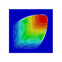
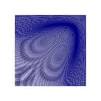
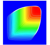
Fig. 1: Burgers equation. Left: ${\mathbb{Q}}_{1}$ FEM with 25 contours; Center left: Final ${\mathbb{Q}}_{1}$ mesh; Center right: ${\mathbb{P}}_{1}$ FEM with 25 contours; Right: Final ${\mathbb{P}}_{1}$ mesh.

6.2.3 Nonconvex flux

Our last scalar example is a nonlinear scalar conservation law with a non-convex flux

(61) $$\partial_{t}u+\nabla{\cdot}{\bm{f}}(u)=0,\quad u_{0}({\bm{x}})=3.25\pi\mathds{1}_{\|{\bm{x}}\|_{\ell^{2}}<1}+0.25\pi.$$

where ${\bm{f}}(u)=(\sin u,\cos u)^{\mathsf{T}}$.

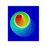
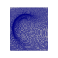
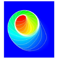
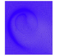
Fig. 2: KPP problem. Left: ${\mathbb{Q}}_{1}$ FEM with 25 contours; Center left: Final ${\mathbb{Q}}_{1}$ mesh; Center right: ${\mathbb{P}}_{1}$ FEM with 25 contours; Right: Final ${\mathbb{P}}_{1}$ mesh.

This test, henceforth referred to as KPP, was proposed in Kurganov et al. [26]. It is a challenging test for many high-order numerical schemes because the solution has a two-dimensional composite wave structure. The initial computational domain is $D^{0}=[-2.5,1.5]\times[-2.0,2.5]$. Note that the background velocity is constant and equal to ${\bm{\beta}}=(\frac{\sqrt{2}}{2},-\frac{\sqrt{2}}{2})^{\mathsf{T}}$. It can be shown that the computational domain keeps a rectangular shape in the time interval $(0,1)$. The computation is done up to time $T=1$ using ${\mathbb{Q}}_{1}$ and ${\mathbb{P}}_{1}$ finite elements on structured meshes $128\times 128$ with $CFL=0.1$. The results are shown in Figure 2

6.3 Compressible Euler equations

We finish the series of tests by solving the compressible Euler equations in $\mathbb{R}^{2}$

(62) $$\begin{cases}\partial_{t}\rho+\nabla{\cdot}(\rho{\bm{u}})&=0,\\ \partial_{t}(\rho{\bm{u}})+\nabla{\cdot}(\rho{\bm{u}}\otimes{\bm{u}}+p\mathds{I})&=0,\\ \partial_{t}E+\nabla{\cdot}({\bm{u}}(E+p))&=0,\end{cases}$$

with an ideal gas equation of state, $p=(\gamma-1)(E-\frac{1}{2}\rho\|{\bm{u}}\|_{\ell^{2}}^{2})$ where $\gamma>1$, and appropriate initial and boundary conditions. The motion of the mesh is done as described in (57) with ${\bm{a}}^{n+1}_{i,\mathrm{Lg}}={\bm{a}}^{n}_{i}+{\tau}{\bm{u}}_{h}^{n}({\bm{a}}_{i}^{n})$ where ${\bm{u}}_{h}^{n}$ is the approximate fluid velocity at time $t^{n}$.

6.3.1 Sod problem

We use the so-called Sod shocktube problem to test the convergence of our algorithm (version-1 only); it is a Riemann problem with the following initial data:

(63) $$\rho_{0}({\bm{x}})=1.0,\quad{\bm{u}}_{0}({\bm{x}})=0.0,\quad p_{0}({\bm{x}})=\mathds{1}_{x_{1}<0.5}+0.1\,\mathds{1}_{x_{1}>0.5}.$$

and $\gamma=1.4$, see e.g., Toro [34, §4.3.3]. The computational domain at the initial time is the unit square $(0,1)^{2}$. Dirichlet boundary conditions are enforced on the left and right sides of the domain and we do not enforce any boundary conditions on the upper and lower sides. The computation is done up to $T=0.2$. Since no wave reaches the left and the right boundaries in the time interval $0<t<T=0.2$, the computational domain remains a square for the whole duration of the simulation. The solution being one-dimensional, the convergence tests are done on five meshes with refinements made only along the $x_{1}$-direction. These meshes have $20{\times}4$, $40{\times}4$, $\ldots$, $1280{\times}4$ cells and are uniform at $t=0$. The results of the convergence test are shown in Table 3. We show in this table the $L^{1}$- and $L^{2}$-norm of the error on the density. The convergence orders are compatible with what is usually obtained in the literature for this problem.

Table 3: SOD problem, ALE, convergence test, $T=0.2$, $CFL=0.1$

	${\mathbb{Q}}_{1}$				${\mathbb{P}}_{1}$
​​# dofs	$L^{2}$-norm		$L^{1}$-norm		$L^{2}$-norm		$L^{1}$-norm
1605	2.47E-02	-	1.51E-02	-	2.82E-02	-	1.77E-02	-
3205	1.84E-02	0.43	9.99E-03	0.60	2.07E-02	0.45	1.15E-02	0.61
6405	1.36E-02	0.42	6.42E-03	0.64	1.56E-02	0.40	7.45E-03	0.63
12805	1.05E-02	0.39	4.07E-03	0.66	1.26E-02	0.32	4.82E-03	0.63

6.4 Noh problem

The last problem that we consider is the so-called Noh problem, see e.g., Caramana et al. [6, §5]. The computational domain at the initial time is $D^{0}=(-1,1)^{2}$ and the initial data is

(64) $$\rho_{0}({\bm{x}})=1.0,\quad{\bm{u}}_{0}({\bm{x}})=-\frac{{\bm{x}}}{\|{\bm{x}}\|_{\ell^{2}}},\quad p_{0}({\bm{x}})=10^{-15}.$$

A Dirichlet boundary condition is enforced on all the dependent variables at the boundary of the domain for the entire simulation. We use $\gamma=\frac{5}{3}$. The solution to this problem is known; for instance, the density is equal to

(65) $$\rho(t,{\bm{x}})=16\mathds{1}_{\{\|{\bm{x}}\|_{\ell^{2}}<\frac{t}{3}\}}+(1+\frac{t}{\|{\bm{x}}\|_{\ell^{2}}})\mathds{1}_{\{\|{\bm{x}}\|_{\ell^{2}}>\frac{t}{3}\}}.$$

The ALE velocity at the boundary of the computational domain is prescribed to be equal to the fluid velocity, i.e., the boundary moves inwards in the radial direction with speed $1$. The final time is chosen to be $T=0.6$ in order to avoid that the shockwave collides with the moving boundary of the computational domain which happens at $t=\frac{3}{4}$ since the shock moves radially outwards with speed $\frac{1}{3}$.

We show in Table 4 the $L^{1}$- and the $L^{2}$-norm of the error on the density for various meshes which are uniform at $t=0$: $30{\times}30$, $60{\times}60$, etc.

Table 4: Noh problem, convergence test, $T=0.6$, $CFL=0.2$

	${\mathbb{Q}}_{1}$				${\mathbb{P}}_{1}$
​​​# dofs	$L^{2}$-norm		$L^{1}$-norm		$L^{2}$-norm		$L^{1}$-norm
961	2.60E-01	-	1.44E-01	-	2.89E-01	-	1.71	-
3721	1.81E-01	0.52	8.45E-01	0.77	2.21E-01	0.39	1.09	0.64
14641	1.16E-01	0.64	4.21E-01	1.01	1.42E-01	0.64	5.15E-01	1.08
58081	7.66E-01	0.60	2.10E-01	0.99	9.39E-01	0.59	2.60E-01	0.99
​231361	5.21E-01	0.56	1.06E-01	0.98	6.33E-01	0.57	1.28E-01	1.02

Preserving the radial symmetry of the solution as best as possible on non-uniform meshes is an important property for Lagrangian hydrocodes in the context of the inertial confinement fusion project, which involves simulating implosion problems, see Caramana et al. [6]. In these problems, mesh-induced violation of the spherical symmetry may artificially trigger the Rayleigh-Taylor instability and thereby may hamper the understanding of the real dynamics of the implosion. We show in the top row of Figure 3 simulations that are done on a uniform mesh composed of $96{\times}96$ square cells for the ${\mathbb{Q}}_{1}$ approximation ($(2{\times}96){\times}(2{\times}96)$ triangular cells for the ${\mathbb{P}}_{1}$ approximation), and we compare them with simulations done on a nonuniform mesh constructed as follows: The initial square $D^{0}$ is divided in four quadrants; in the bottom left quadrant the mesh is composed of $32{\times}32$ square cells; in the top left quadrant the mesh is composed of $32{\times}64$ rectangular cells; in the top right quadrant the mesh is composed of $64{\times}64$ square cells; the bottom right quadrant is composed of $64{\times}32$ rectangular cells. This is a generic test for many Lagrangian hydrocodes, see e.g., Dobrev et al. [13, §8.4]. We notice a slight break of symmetry, but the solution does not develop any Rayleigh-Taylor-type instability as it is often the case for many other Lagrangian algorithms.

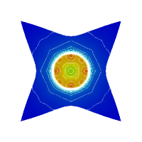
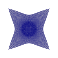
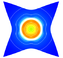
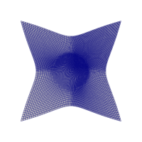
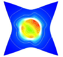
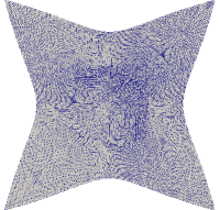
Fig. 3: Noh problem. Uniform meshes in top row, nonuniform meshes in bottom row. From left to right: density field with ${\mathbb{Q}}_{1}$ approximation (25 contour lines); mesh with ${\mathbb{Q}}_{1}$ approximation; density field with ${\mathbb{P}}_{1}$ approximation (25 contour lines); mesh with ${\mathbb{P}}_{1}$ approximation.

We show in Figure 4 a zoom around the center of the computational domain for both the ${\mathbb{Q}}_{1}$ and the ${\mathbb{P}}_{1}$ approximations. We notice a slight motion of the center, but there is no dramatic breakdown of the structure of the solution.

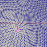
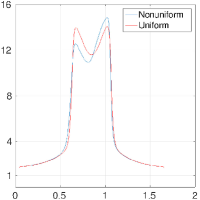
Fig. 4: Noh problem. From left to right: Zoom around the center of the nonuniform ${\mathbb{Q}}_{1}$ mesh at $T=0.6$ (notice the small displacement of the center); Cross section along the line connecting the points $(-1,-1)$ and $(1,1)$ for the ${\mathbb{Q}}_{1}$ solutions on the uniform mesh and on the nonuniform mesh; Zoom around the center of the nonuniform ${\mathbb{P}}_{1}$ mesh at $T=0.6$; Cross section along the line connecting the points $(-1,-1)$ and $(1,1)$ for the ${\mathbb{P}}_{1}$ solutions on the uniform mesh and on the nonuniform mesh;

7 Concluding remarks

In this paper we have developed a framework for constructing ALE algorithms using continuous finite elements. The method is invariant domain preserving on any mesh in arbitrary space dimension. The methodology applies to any hyperbolic system which has such intrinsic property. If the system at hand has an entropy pair, then the method also satisfies a discrete entropy inequality. The time accuracy of one of the methods (scheme 1) can be increased by using SSP time discretization techniques. This makes the method appropriate to use as a safeguard when constructing high-order accurate discretization of the system which may violate the invariant domain property. The equivalence between the conservative and non-conservative formulations implies the DGCL condition (preservation of constant states). The new methods have been tested on a series of benchmark problems and the observed convergence orders and numerical performance are compatible with what is reported in the literature.

References

- Ainsworth [2014] M. Ainsworth. Pyramid algorithms for Bernstein-Bézier finite elements of high, nonuniform order in any dimension. SIAM J. Sci. Comput., 36(2):A543–A569, 2014.
- Bangerth et al. [2007] W. Bangerth, R. Hartmann, and G. Kanschat. deal.II – a general purpose object oriented finite element library. ACM Trans. Math. Softw., 33(4):24/1–24/27, 2007.
- Barlow [2007] A. Barlow. A compatible finite element multi-material ALE hydrodynamics algorithm. Internat. J. Numer. Methods Fluids, 56:953–964, 2007.
- Boscheri and Dumbser [2014] W. Boscheri and M. Dumbser. A direct arbitrary-Lagrangian-Eulerian ADER-WENO finite volume scheme on unstructured tetrahedral meshes for conservative and non-conservative hyperbolic systems in 3D. J. Comput. Phys., 275:484–523, 2014.
- Bressan [2000] A. Bressan. Hyperbolic systems of conservation laws, volume 20 of Oxford Lecture Series in Mathematics and its Applications. Oxford University Press, Oxford, 2000. The one-dimensional Cauchy problem.
- Caramana et al. [1998] E. Caramana, M. Shashkov, and P. Whalen. Formulations of artificial viscosity for multi-dimensional shock wave computations. J. Comput. Phys., 144(1):70–97, 1998.
- Caramana and Loubère [2006] E. J. Caramana and R. Loubère. “Curl-”: a vorticity damping artificial viscosity for essentially irrotational Lagrangian hydrodynamics calculations. J. Comput. Phys., 215(2):385–391, 2006.
- Carré et al. [2009] G. Carré, S. Del Pino, B. Després, and E. Labourasse. A cell-centered Lagrangian hydrodynamics scheme on general unstructured meshes in arbitrary dimension. J. Comput. Phys., 228(14):5160–5183, 2009.
- Chen [2005] G.-Q. Chen. Euler equations and related hyperbolic conservation laws. In Evolutionary equations. Vol. II, Handb. Differ. Equ., pages 1–104. Elsevier/North-Holland, Amsterdam, 2005.
- Cheng and Shu [2014] J. Cheng and C.-W. Shu. Positivity-preserving Lagrangian scheme for multi-material compressible flow. J. Comput. Phys., 257(part A):143–168, 2014.
- Chueh et al. [1977] K. N. Chueh, C. C. Conley, and J. A. Smoller. Positively invariant regions for systems of nonlinear diffusion equations. Indiana Univ. Math. J., 26(2):373–392, 1977.
- Dafermos [2000] C. M. Dafermos. Hyperbolic conservation laws in continuum physics, volume 325 of Grundlehren der Mathematischen Wissenschaften [Fundamental Principles of Mathematical Sciences]. Springer-Verlag, Berlin, 2000.
- Dobrev et al. [2012] V. Dobrev, T. Kolev, and R. Rieben. High-order curvilinear finite element methods for Lagrangian hydrodynamics. SIAM J. Sci. Comput., 34(5):B606–B641, 2012.
- Farhat et al. [2001] C. Farhat, P. Geuzaine, and C. Grandmont. The discrete geometric conservation law and the nonlinear stability of ALE schemes for the solution of flow problems on moving grids. J. Comput. Phys., 174(2):669–694, 2001.
- Ferracina and Spijker [2005] L. Ferracina and M. N. Spijker. An extension and analysis of the Shu-Osher representation of Runge-Kutta methods. Math. Comp., 74(249):201–219, 2005.
- Frid [2001] H. Frid. Maps of convex sets and invariant regions for finite-difference systems of conservation laws. Arch. Ration. Mech. Anal., 160(3):245–269, 2001.
- Gastaldi [2001] L. Gastaldi. A priori error estimates for the Arbitrary Lagrangian Eulerian formulation with finite elements. J. Num. Math., 9(2):123–156, 2001.
- Gottlieb et al. [2009] S. Gottlieb, D. I. Ketcheson, and C.-W. Shu. High order strong stability preserving time discretizations. J. Sci. Comput., 38(3):251–289, 2009.
- Guermond and Popov [2015a] J.-L. Guermond and B. Popov. Fast estimation of the maximum wave speed in the Riemann problem for the euler equations. 2015a. arXiv:1511.02756, Submitted.
- Guermond and Popov [2015b] J.-L. Guermond and B. Popov. Invariant domains and first-order continuous finite element approximation for hyperbolic systems. 2015b. arXiv:1509.07461, Submitted.
- Guermond et al. [2016] J.-L. Guermond, B. Popov, and V. Tomov. Entropy-viscosity method for the single material euler equations in Lagrangian frame. Computer Methods in Applied Mechanics and Engineering, 300:402 – 426, 2016.
- Guillard and Farhat [2000] H. Guillard and C. Farhat. On the significance of the geometric conservation law for flow computations on moving meshes. Comput. Methods Appl. Mech. Engrg., 190(11-12):1467–1482, 2000.
- Higueras [2005] I. Higueras. Representations of Runge-Kutta methods and strong stability preserving methods. SIAM J. Numer. Anal., 43(3):924–948, 2005.
- Hoff [1985] D. Hoff. Invariant regions for systems of conservation laws. Trans. Amer. Math. Soc., 289(2):591–610, 1985.
- Kolev and Rieben [2009] T. Kolev and R. Rieben. A tensor artificial viscosity using a finite element approach. J. Comput. Phys., 228(22):8336–8366, 2009.
- Kurganov et al. [2007] A. Kurganov, G. Petrova, and B. Popov. Adaptive semidiscrete central-upwind schemes for nonconvex hyperbolic conservation laws. SIAM J. Sci. Comput., 29(6):2381–2401 (electronic), 2007.
- Lai and Schumaker [2007] M.-J. Lai and L. L. Schumaker. Spline functions on triangulations, volume 110 of Encyclopedia of Mathematics and its Applications. Cambridge University Press, Cambridge, 2007.
- Lax [1954] P. Lax. Weak solutions of nonlinear hyperbolic equations and their numerical computation. Comm. Pure Appl. Math., 7:159–193, 1954.
- Lax [1957] P. D. Lax. Hyperbolic systems of conservation laws. II. Comm. Pure Appl. Math., 10:537–566, 1957.
- Lipnikov and Shashkov [2010] K. Lipnikov and M. Shashkov. A framework for developing a mimetic tensor artificial viscosity for Lagrangian hydrocodes on arbitrary polygonal meshes. J. Comput. Phys., 229(20):7911–7941, 2010.
- Loubère et al. [2010] R. Loubère, P.-H. Maire, M. Shashkov, J. Breil, and S. Galera. ReALE: A reconnection-based arbitrary-Lagrangian-Eulerian method. Journal of Computational Physics, 229(12):4724 – 4761, 2010.
- Scovazzi et al. [2008] G. Scovazzi, E. Love, and M. Shashkov. Multi-scale Lagrangian shock hydrodynamics on Q1/P0 finite elements: Theoretical framework and two-dimensional computations. Comput. Methods Appl. Mech. Engrg., 197:1056–1079, 2008.
- Shashkov and Campbell [2001] M. Shashkov and J. Campbell. A tensor artificial viscosity using a mimetic finite difference algorithm. J. Comput. Phys., 172(2):739–765, 2001.
- Toro [2009] E. F. Toro. Riemann solvers and numerical methods for fluid dynamics. Springer-Verlag, Berlin, third edition, 2009. A practical introduction.
- Vilar et al. [2014] F. Vilar, P.-H. Maire, and R. Abgrall. A discontinuous Galerkin discretization for solving the two-dimensional gas dynamics equations written under total Lagrangian formulation on general unstructured grids. J. Comput. Phys., 276(0):188 – 234, 2014.
- Wells et al. [2005] B. Wells, M. Baines, and P. Glaister. Generation of Arbitrary Lagrangian-Eulerian (ALE) velocities, based on monitor functions, for the solution of compressible uid equations. Int. J. Numer. Meth. Fluids, 47:1375–1381, 2005.
- Yang and Mavriplis [2005] Z. Yang and D. J. Mavriplis. Unstructured dynamic meshes with higher-order time integration schemes for the unsteady Navier-Stokes equations. AIAA Paper 2005–1222, 2005.