Network Unfolding Map by Vertex-Edge Dynamics Modeling

Abstract

The emergence of collective dynamics in neural networks is a mechanism of the animal and human brain for information processing. In this paper, we develop a computational technique using distributed processing elements in a complex network, which are called particles, to solve semi-supervised learning problems. Three actions govern the particles’ dynamics: generation, walking, and absorption. Labeled vertices generate new particles that compete against rival particles for edge domination. Active particles randomly walk in the network until they are absorbed by either a rival vertex or an edge currently dominated by rival particles. The result from the model evolution consists of sets of edges arranged by the label dominance. Each set tends to form a connected subnetwork to represent a data class. Although the intrinsic dynamics of the model is a stochastic one, we prove there exists a deterministic version with largely reduced computational complexity; specifically, with linear growth. Furthermore, the edge domination process corresponds to an unfolding map in such way that edges “stretch” and “shrink” according to the vertex-edge dynamics. Consequently, the unfolding effect summarizes the relevant relationships between vertices and the uncovered data classes. The proposed model captures important details of connectivity patterns over the vertex-edge dynamics evolution, in contrast to previous approaches which focused on only vertex or only edge dynamics. Computer simulations reveal that the new model can identify nonlinear features in both real and artificial data, including boundaries between distinct classes and overlapping structures of data.

I Introduction

Semi-supervised learning (SSL) is one of the machine learning paradigms, which lies between the unsupervised and supervised learning paradigms. In SSL problems, both unlabeled and labeled data are taken into account in class or cluster formation and prediction processes [1, 2]. In real-world applications, we usually have partial knowledge on a given dataset. For example, we certainly do not know every movie actor except a few famous ones; in a large-scale social network, we just know some friends; in biological domain, we are far away from completely obtaining a figure of the functions of all genes, but we know the functions of some of them. Sometimes, although we have a complete or almost complete knowledge of a dataset, labeling it by hand is lengthy and expensive. So it is necessary to restrict the labeling scope. For these reasons, partially labeled datasets are often encountered. In this sense, supervised and unsupervised learning can be considered as extreme and special cases of semi-supervised learning. Many semi-supervised learning techniques have been developed, including generative models [3], discriminative models [4], clustering and labeling techniques [5], multi-training [6], low-density separation models [7], and graph-based methods [8, 9, 10]. Among the approaches listed above, graph-based SSL has triggered much attention. In this case, each data instance is represented by a vertex and is linked to other vertices according to a predefined affinity rule. The labels are propagated to the whole graph using a particular optimization heuristic [11].

Complex networks are large-scale graphs with nontrivial topology [12]. Such networks introduce a powerful tool to describe the interplay of topology, structure, and dynamics of complex systems [12, 13]. Therefore, they provide a groundbreaking mechanism to help us understand the behavior of many real systems. Networks also turn out to be an important mechanism for data representation and analysis [14]. Interpreting data sets as complex networks grant us to access the inter-relational nature of data items further. For this reason, we consider the network-based approach for SSL in this work. However, the above-mentioned network-based approach focuses on the optimization of the label propagation result and pays little attention to the detailed dynamics of the learning process itself. On the other hand, it is well-known that collective neural dynamics generate rich information, and such a redundant processing handles the adaptability and robustness of the learning process. Moreover, traditional graph-based techniques have high computational complexity, usually at cubic order [15]. A common strategy to overcome this disadvantage is using a set of sparse prototypes derived from the data [10]. However, such a sampling process usually loses information of the original data.

Taking into account the facts above, we study a new type of dynamical competitive learning mechanism in a complex network, called particle competition. Consider a network where several particles walk and compete to occupy as many vertices as possible while attempting to reject rival particles. Each particle performs a combined random and preferential walk by choosing a neighbor vertex to visit. Finally, it is expected that each particle occupies a subset of vertices, called a community of the network. In this way, community detection is a direct result of the particle competition. The particle competition model was originally proposed in [16] and extended for the data clustering task in [17]. Later, it has been applied to semi-supervised learning [18, 19] where the particle competition is formally represented by a nonlinear stochastic dynamical system. In all the models mentioned above, the authors concern vertex dynamics—how each vertex changes its state (the level of dominance of each particle). Intuitively, vertex dynamics is a rough modeling of a network because each vertex can have several edges. A problem with the data analysis in this approach is the overlapping nature of the vertices, where a data item (a vertex in the networked form) can belong to more than one class. Therefore, it is interesting to know how each edge changes its state in the competition process to acquire detailed knowledge of the dynamical system.

In this paper, we propose a transductive semi-supervised learning model that employs a vertex–edge dynamical system in complex networks. In this dynamical system, namely Labeled Component Unfolding system, particles compete for edges in a network. Subnetworks are generated with the edges grouped by class dominance. Here, we call each subnetwork an unfolding. The learning model employs the unfoldings to classify unlabeled data. The proposed model offers satisfactory performance on semi-supervised learning problems, in both artificial and real dataset. Also, it has shown to be suitable for detecting overlapping regions of data points by simply counting the edges dominated by each class of particles. Moreover, it has low computational complexity order.

In comparison to the original particle competition models and other graph-based semi-supervised learning techniques, the proposed one presents the following salient features:

Particle competition dynamics occurs on nodes as well as on edges

The inclusion of the edge domination model can give us more detailed information to capture connectivity pattern of the input data. This is because there are much more edges than vertices even in a sparse network. Consequently, the proposed model has the benefit of granting essential information concerning overlapping vertices. Computer simulations show the proposed technique achieves a good classification accuracy and it is suitable for situations with a small number of labeled samples.

In the proposed model, particles are continuously generated and removed from the system

Such a feature contrasts to previous particle competition models that incorporate a preferential walking mechanism where particles tend to avoid rival particles. As a consequence, the number of active particles in the system varies over time. It is worth noting that the elimination of preferential walking mechanism largely simplifies the dynamical rules of particle competition model. Now, the new model is characterized by the competition of only random walking particles, which, in turn, permits us to find out an equivalent deterministic version. The original particle competition model is intrinsically stochastic. Then, each run may generate a different result. Consequently, it has high computational cost. In this work, we find out a deterministic system with running time independent of the number of particles, and we demonstrate that it is mathematically equivalent to the stochastic model. Moreover, the deterministic model has linear time order and ensures stable learning. In other words, the model generates the same output for each run with the same input. Furthermore, the system is simpler and easier to be understood and implemented. Thus, the proposed model is more efficient than the original particle competition model.

There is no explicit objective function

In classical graph-based semi-supervised learning techniques, usually, an objective function is defined for optimization. Such function considers not only the label information, but also the semi-supervised assumptions of smoothness, cluster, or manifold. In particle competition models, we do not need to define an objective function. Instead, dynamical rules which govern the time evolution of particles and vertices (or edges) are defined. Those dynamical rules mimic the phenomena observed in some natural and social systems, such as resource competition among animals, territory exploration by humans (or animals), election campaigns, etc. In other words, the particle competition technique is typically inspired by nature. In such kind of technique, we have focused on behavior modeling instead of objective modeling. Certain objectives can be achieved if the corresponding behavioral rules are properly defined. In this way, we may classify classical graph-based semi-supervised learning techniques as objective-based design and the particle competition technique as behavior-based design.

The remainder of this paper is organized as follows. The proposed particle competition system is studied in Section II. Our transductive semi-supervised learning model is represented in Section III. In Section IV, results of computer simulations are shown to assess the proposed model performance on both artificial and real-world datasets. Finally, Section V concludes this paper.

II Labeled Component Unfolding system

In this section, we give an introduction to the Labeled Component Unfolding (LCU) system—a particle competition system for edge domination—explaining its basic design. Whenever pertinent, we go into detail for further clarification.

II-A Overview

We consider a complex network expressed by a simple, unweighted, undirected graph $G=(\mathcal{V},\mathcal{E})$, where $\mathcal{V}$ is the set of vertices and $\mathcal{E}\subseteq\mathcal{V}\times\mathcal{V}$ is the set of edges. If two vertices are considered similar, an edge connects them. The network contains $\left\lvert\mathcal{V}\right\rvert=l+u$ vertices that can be either labeled or unlabeled data points. The set $\mathcal{L}=\{v_{1},\dots,v_{l}\}$ contains the labeled vertices, where a vertex $v_{i}\in\mathcal{L}$ has a label $y_{i}\in\{1,\ldots,C\}$. We also use the terms label and class synonymously—if a vertex is labeled with $c$, we say this vertex belongs to class $c$. The set $\mathcal{U}=\{v_{l+1},\dots,v_{l+u}\}$ contains the unlabeled vertices. We suppose that $l\ll u$. Thus, we have that $\mathcal{L}\,\cap\,\mathcal{U}=\emptyset$ and $\mathcal{V}=\mathcal{L}\,\cup\,\mathcal{U}$. The network is represented by the adjacency matrix $A=(a_{ij})$ where $a_{ij}=a_{ji}=1$ if $v_{i}$ is connected to $v_{j}$. We denote $(i,j)$ as the edge between vertices $v_{i}$ and $v_{j}$. For practical reasons, we consider a connected network, and there is at least one labeled vertex of each class.

In this model, particles are objects that flow within the network while carrying a label. Labeled vertices are sources for particles of the same class and sinks for particles of other classes. After a particle is released, it randomly walks the network. There is equal probability among adjacent vertices to be chosen as the next vertex to be visited by the particle. Consider that a particle is in $v_{i}$, it decides to move to $v_{j}$ with probability

$$\frac{a_{ij}}{\operatorname{deg}{v_{i}}}$$

with $\operatorname{deg}{v_{i}}$ denoting the degree of $v_{i}$.

In each step, at the moment that a particle decides to move to a next vertex, it can be absorbed (removed from the system). If a particle is not absorbed, we say that it has survived and it remains active; and if it survives, then it continues walking. Otherwise, the particle is absorbed and ceases to affect the system. The absorption depends on the level of subordination and domination of a class against all other classes in the edges.

To determine the level of domination and subordination of each class in an edge, we take into account the active particles in the system. The current directed domination $\tilde{n}^{c}_{ij}(t)$ is the number of active particles belonging to class $c$ that decided to move from $v_{i}$ to $v_{j}$ at time $t$ and survived. Similarly, the current relative subordination $\tilde{\sigma}^{c}_{ij}$ is the fraction of active particles that do not belong to class $c$ and have successfully passed through edge $(i,j)$, regardless of direction, at time $t$. Mathematically, we define the latter as

$$\tilde{\sigma}^{c}_{ij}\coloneqq\begin{dcases*}1-\frac{\tilde{n}^{c}_{ij}+\tilde{n}^{c}_{ji}}{\sum_{q=1}^{C}{\tilde{n}^{q}_{ij}+\tilde{n}^{q}_{ji}}}&if $\sum_{q=1}^{C}{\tilde{n}^{q}_{ij}+\tilde{n}^{q}_{ji}}>0$,\\ 1-\frac{1}{C}&otherwise.\end{dcases*}$$

The survival of a particle depends on the current relative subordination of the edge and the destination vertex. If a particle decides to move into a sink, it will be absorbed with probability 1. If the destination vertex is not a sink, its survival probability is

$$1-\lambda\tilde{\sigma}^{c}_{ij}(t)$$

where $\lambda\in[0,1]$ is a parameter for characterizing the competition level.

A source generates particles according to its degree and the current number of active particles in the system. Let $\tilde{n}^{c}(t)$ be the number of active particles belonging to class $c$ in the system at time $t$, a source generates new particles if $\tilde{n}^{c}(t)<\tilde{n}^{c}(0)$.

Let $\mathcal{G}^{c}=\left\{v_{i}\middle|v_{i}\in\mathcal{L}\mbox{ and }y_{i}=c\right\}$ be the set of sources for particles that belong to class $c$, the number of newly generated particles belonging to class $c$ in $v_{i}$ at time $t$ follows the distribution

$$\begin{dcases*}\mathrm{B}\!\left(\tilde{n}^{c}(0)-\tilde{n}^{c}(t),~{}\rho^{c}_{i}\right)&if $\tilde{n}^{c}(0)-\tilde{n}^{c}(t)>0$,\\ \mathrm{B}(1,0)&otherwise,\end{dcases*}$$

where

$$\rho^{c}_{i}\coloneqq\begin{dcases*}\frac{\operatorname{deg}{v_{i}}}{\sum_{v_{j}\in\mathcal{G}^{c}}{\operatorname{deg}{v_{j}}}}&if $v_{i}\in\mathcal{G}^{c}$,\\ 0&otherwise,\end{dcases*}$$

and $\mathrm{B}(n,p)$ is a binomial distribution. In other words, if the number of active particles is fewer than the initial number of particles, $\tilde{n}^{c}(0)$, each source performs $\tilde{n}^{c}(0)-\tilde{n}^{c}(t)$ trials with probability $\rho^{c}_{i}$ of generating a new particle.

Therefore, the expected number of new particles belonging to class $c$ in $v_{i}$ at time $t$ is

$$\begin{dcases}\rho^{c}_{i}\left(\tilde{n}^{c}(0)-\tilde{n}^{c}(t)\right)&\mbox{if }\tilde{n}^{c}(0)-\tilde{n}^{c}(t)>0\mbox{,}\\ 0&\mbox{otherwise.}\end{dcases}$$

We are interested in the total number of visits of particles of each class to each edge. Thus, we introduce the cumulative domination $\tilde{\delta}^{c}_{ij}(t)$ that is the total number of particles belonging to class $c$ that passed through edge $(i,j)$ up to time $t$. Mathematically, this is defined as

$$\tilde{\delta}^{c}_{ij}(t)\coloneqq\sum_{\tau=1}^{t}{\tilde{n}^{c}_{ij}(\tau)\,\mbox{.}}$$ (1)

Using the cumulative domination, we can group the edges by class domination. For each class $c$, the subset $\mathcal{E}^{c}(t)\subseteq\mathcal{E}$ is

$$\mathcal{E}^{c}(t)\coloneqq\left\{\mbox{$(i,j)$}\middle|\operatorname*{arg\,max}_{q}\!{\left(\tilde{\delta}^{q}_{ij}(t)+\tilde{\delta}^{q}_{ji}(t)\right)=c}\right\}\mbox{.}$$

We define the subnetwork

$$G^{c}(t)\coloneqq\left(\mathcal{V},\mathcal{E}^{c}(t)\right)$$ (2)

as the unfolding of network $G$ according to class $c$ at time $t$. We interpret the unfolding as a subspace with the most relevant relationships for a given class. We use the available information in these subnetworks for the study of overlapping regions and for semi-supervised learning.

II-B An Illustrative Example

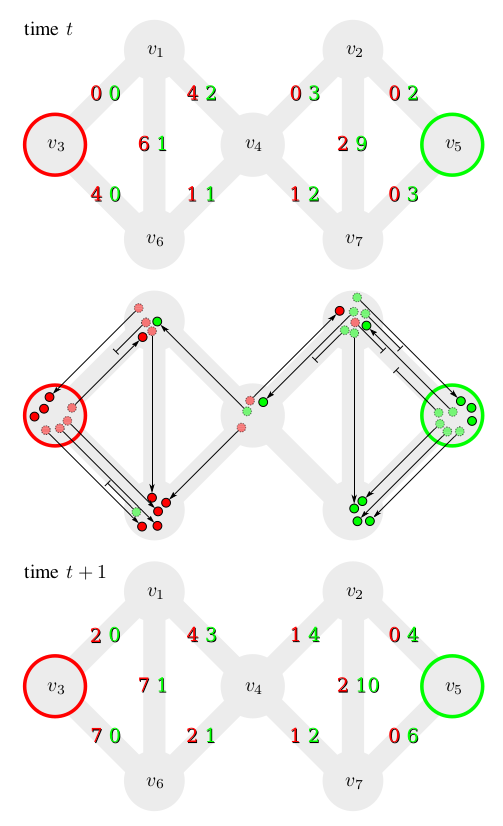
Figure 1: Illustration of one iteration of the system’s evolution. The network consists of 7 vertices and 10 edges; each color represents a label of a particle or a source. The first and the third networks depict the cumulative domination before and after the iteration. The cumulative domination is the number of visits of particles to an edge since the initial state. In the second network, particles are depicted in small circles. Active particles at time $t$ are depicted in dashed borders, whereas active particles at time $t+1$ are in full borders. An arrow indicates a particle movement, while an interrupted line indicates that the particle has been absorbed when trying to move through an edge. Particles without an adjacent arrow are generated by the sources at time $t+1$.

One iteration of the system’s evolution is illustrated by Figure 1. The considered system contains 22 active particles at time $t$ and 20 at time $t+1$. In an iteration, each particle moves to a neighbor vertex, without preference. The movement of a particle is indicated by an arrow. An interrupted line indicates an edge in which the coming particle is absorbed. A total of 6 particles are absorbed during this iteration, and the sources have generated 4 new particles.

At time $t$, for example, one of the red particles passing through edge $(1,3)$ is absorbed due to a current edge dominance of 0.5 in that edge (one red particle and one green particle). Conversely, all green particles that moved through edge $(5,7)$ remain active at time $t+1$. Since there is no rival particle (red particle) passing through this edge, the updated value of the current edge dominance is 1 and 0 for green and red classes, respectively.

In edge $(2,4)$, one red and two green particles chose to pass through. One green particle is absorbed without affecting the new current level of dominance. Since one particle of each class successfully passed through edge $(2,4)$, the new current level of dominance on this edge is 0.5. The same occurs for edge $(4,7)$ where no particles have passed through and, thus, the current level of dominance is set equally among all classes.

In edges $(2,5)$ and $(3,6)$, particles have tried to move into a source of rival particles (sinks). These particles are absorbed independently from the current level of dominance.

Our edge-centric system can measure the overlapping nature of the $v_{4}$ by counting the edges dominated by each class, while a vertex-centric approach would have lost such information.

II-C Mathematical Modeling

Formally, we define the Labeled Component Unfolding system as a dynamical system $\tilde{X}(t)$. The state of the system is

$$\tilde{X}(t)\coloneqq\begin{bmatrix}\mathbf{\tilde{n}}^{c}(t)=\big{[}\tilde{n}^{c}_{i}(t)\big{]}_{i}\\[7.22743pt] \tilde{\Delta}^{c}(t)=\big{(}\tilde{\delta}^{c}_{ij}(t)\big{)}_{i,j}\end{bmatrix}\,\mbox{,}$$ (3)

where $\mathbf{\tilde{n}}^{c}(t)$ is a vector, and each element $\tilde{n}^{c}_{i}(t)$ is the number of active particles belonging to class $c$ in $v_{i}$ at time $t$. Furthermore, $\tilde{\Delta}^{c}(t)$ is a matrix whose elements $\tilde{\delta}^{c}_{ij}(t)$ are given by Equation 1.

Let $\tilde{g}^{c}_{i}(t)$ and $\tilde{a}^{c}_{i}(t)$ be, respectively, the number of particles generated and absorbed by $v_{i}$ at time $t$. The evolution function $\tilde{\phi}$ of the dynamical system is

$$\tilde{\phi}:\begin{dcases}\tilde{n}^{c}_{i}(t+1)=\tilde{n}^{c}_{i}(t)+\sum_{j}{\left(\tilde{n}^{c}_{ji}(t+1)-\tilde{n}^{c}_{ij}(t+1)\right)}\\ \phantom{\tilde{n}^{c}_{i}(t+1)=\tilde{n}^{c}_{i}(t)}+\tilde{g}^{c}_{i}(t+1)-\tilde{a}_{i}^{c}(t+1)\,\mbox{.}\phantom{\sum_{j}{}}\\ \tilde{\delta}^{c}_{ij}(t+1)=\tilde{\delta}^{c}_{ij}(t)+\tilde{n}^{c}_{ij}(t+1)\,\mbox{.}\end{dcases}$$

Intuitively, the number $\tilde{n}^{c}_{i}$ of active particles that are in a vertex is the total number of particles arriving, $\tilde{n}^{c}_{ji}$, minus the number of particles leaving, $\tilde{n}^{c}_{ij}$, or being absorbed, $\tilde{a}_{i}^{c}$; additionally for labeled vertices, the number of generated particles, $\tilde{g}^{c}_{i}$. Moreover, to calculate the total number $\tilde{\delta}^{c}_{ij}$ of visits of particles to an edge, we simply add up the number $\tilde{n}^{c}_{ij}$ at each time. Values $\tilde{n}^{c}_{ij}$, $\tilde{g}^{c}_{i}$, and $\tilde{a}^{c}_{i}$ are obtained stochastically according to the dynamics of walking, absorption, and generation.

The initial state of the system is given by an arbitrary number $\tilde{n}^{c}_{i}(0)$ of initial active particles and

$$\begin{dcases}\tilde{n}^{c}_{ij}(0)=0\,\mbox{,}\\ \tilde{\delta}^{c}_{ij}(0)=0\,\mbox{.}\end{dcases}$$

To achieve the desirable network unfolding, it is necessary to average the results of several simulations of the system with a very large number of initial particles $\tilde{n}^{c}_{i}(0)$. Thus, the computational cost of such a simulation is very high. Conversely, we provide an alternative system $X(t)$ that achieves similar results in a deterministic manner. More details will follow.

II-D Alternative Mathematical Modeling

Consider the dynamical system

$$X(t)\coloneqq\begin{bmatrix}\mathbf{n}^{c}(t)=\big{[}n^{c}_{i}(t)\big{]}_{i}\\[7.22743pt] N^{c}(t)=\big{(}n^{c}_{ij}(t)\big{)}_{i,j}\\[7.22743pt] \Delta^{c}(t)=\big{(}\delta^{c}_{ij}(t)\big{)}_{i,j}\end{bmatrix}\,\mbox{,}$$ (4)

where $\mathbf{n}^{c}(t)$ is a row vector whose elements $n^{c}_{i}(t)$ give the population of particles with label $c$ in each vertex $v_{i}$ at time $t$. These values are associated to the number of active particles $\tilde{n}^{c}_{i}$ of system $\tilde{X}$. The elements $n^{c}_{ij}(t)$ and $\delta^{c}_{ij}(t)$ of the sparse matrices $N^{c}(t)$ and $\Delta^{c}(t)$ are related to the current directed domination, $\tilde{n}^{c}_{ij}$, and the cumulative domination, $\tilde{\delta}^{c}_{ij}$, respectively. In other words, $n^{c}_{ij}(t)$ gives the number of particles of class $c$ that moved from $v_{i}$ to $v_{j}$ at time $t$, while $\delta^{c}_{ij}(t)$ gives the total number up to time $t$.

The system $X$ is a nonlinear Markovian dynamical system with the deterministic evolution function

$$\phi\colon\begin{dcases}\mathbf{n}^{c}(t+1)=\mathbf{n}^{c}(t)\times P^{c}(X(t))+\mathbf{g}^{c}(X(t))\\ N^{c}(t+1)=\operatorname{diag}{\mathbf{n}^{c}(t)}\times P^{c}(X(t))\\ \Delta^{c}(t+1)=\Delta^{c}(t)+N^{c}(t+1)\,\mbox{,}\end{dcases}$$ (5)

where $\operatorname{diag}{\mathbf{v}}$ is a square matrix with the elements of vector $\mathbf{v}$ on the main diagonal and $\times$ stands for the vector-matrix product.

The function $P^{c}(X(t))$ of the system $X$ at time $t$ gives a square matrix whose elements are

where

$$\sigma^{c}_{ij}\!\left(X(t)\right)\coloneqq\begin{dcases*}1-\frac{n^{c}_{ij}(t)+n^{c}_{ji}(t)}{S}&if $S>0$,\\ 1-\frac{1}{C}&otherwise,\end{dcases*}\\ \mbox{with }S=\sum_{q=1}^{C}{n^{q}_{ij}(t)+n^{q}_{ji}(t)}\mbox{.}$$ (7)

Given that we know the initial state $X(0)$ of the system, the function $\mathbf{g}^{c}(X(t))$ of the system $X$ at time $t$ returns a row vector where the $i$-th element is

$$g^{c}_{i}(X(t))\coloneqq\rho^{c}_{i}\max\!\left\{0,\;\mathbf{1}\cdot\mathbf{n}^{c}(0)-\mathbf{1}\cdot\mathbf{n}^{c}(t)\right\}\mbox{,}$$ (8)

where $\mathbf{1}$ is a row vector whose elements are $1$, and $\cdot$ stands for the inner product between vectors.

The initial state of the system $X$ is given by an arbitrary population size $n^{c}_{i}(0)$ of initial active particles and

$$\begin{dcases}n^{c}_{ij}(0)=0\,\mbox{,}\\ \delta^{c}_{ij}(0)=0\,\mbox{.}\end{dcases}$$

If the initial number of particles in each vertex in system $\tilde{X}$ is proportional to the initial population size in system $X$, we provide evidence that the unfolding result tends to be the same for both systems—represented by Equation 3 and Equation 4, respectively—, as $\tilde{n}^{c}_{i}(0)\rightarrow\infty$ for all $c\in\{1,\dots,C\}$ and $i\in\{1,\dots,\left\lvert\mathcal{V}\right\rvert\}$.

II-E Mathematical Analysis

In the previous subsections, we modeled two possibly equivalent systems, $X$ and $\tilde{X}$. In this section, we present mathematical results that prove the equivalence of the two systems under certain assumptions.

Theorem 1.

Systems $X$ and $\tilde{X}$ are asymptotically equivalent if the following conditions hold:

$$\mathrm{E}\!\left[\tilde{\sigma}^{c}_{ij}(t)\right]\rightarrow 1-\frac{\mathrm{E}\!\left[\tilde{n}^{c}_{ij}(t)\right]+\mathrm{E}\!\left[\tilde{n}^{c}_{ji}(t)\right]}{\sum_{q=1}^{C}{\mathrm{E}\!\left[\tilde{n}^{q}_{ij}(t)\right]+\mathrm{E}\!\left[\tilde{n}^{q}_{ji}(t)\right]}}\mbox{ and}$$

$$\mathrm{E}\!\left[\tilde{g}^{c}_{i}(t+1)\right]\rightarrow\rho^{c}_{i}\max\!\left\{0,\;\tilde{n}^{c}(0)-\mathrm{E}\!\left[\tilde{n}^{c}(t)\right]\right\}\mbox{ as}$$

$$\tilde{n}^{c}_{i}(0)\rightarrow\infty\mbox{,}$$

for all $i,j\in\mathcal{V}$, $t>0$, and $c\in\{1,\dots,C\}$, we have

$$n^{c}_{i}(t)=\kappa\mathrm{E}\!\left[\tilde{n}^{c}_{i}(t)\right]\mbox{, }n^{c}_{ij}(t)=\kappa\mathrm{E}\!\left[\tilde{n}^{c}_{ij}(t)\right]\mbox{, and}$$

$$\delta^{c}_{ij}(t)=\kappa\mathrm{E}\!\left[\tilde{\delta}^{c}_{ij}(t)\right]\mbox{, }$$

for some $k>0$ constant.

In order to prove Theorem 1, we study the following mechanisms of the particle competition system:

II-E1 Particle motion and absorption

In the proposed system, each particle moves independently from the others. Particle’s movement through an edge affects the absorption of rival particles only in the next iteration. Such conditions are favorable to naturally regard the system’s evolution in terms of the distribution of particles over the network. Next, we present a formal model for particle movement.

Let $\mathrm{I}_{ij}(p,~{}t+1)$ be a discrete random variable that is 1 if particle $p$ was in $v_{i}$ at time $t$ and moved into $v_{j}$ at time $t+1$; and it is 0 otherwise. Since each particle in a vertex moves independently, we can write this probability in terms of a particle’s class; that is, $\mathrm{I}^{c}_{ij}(t+1)=\mathrm{I}_{ij}(p,~{}t+1)$ for any particle $p$ that belongs to class $c$ and is in $v_{i}$ at time $t$.

The probability $\Pr\!\left[\mathrm{I}^{c}_{ij}(t+1)=1\right]$ is affected by the movement decision of a particle and whether it was absorbed after the decision. By formulation, in dynamical system $\tilde{X}$ the conditional probability, given that $\tilde{\sigma}^{c}_{ij}(t)=\xi$, is

$$\Pr\!\left[\mathrm{I}^{c}_{ij}(t+1)=1\middle|\tilde{\sigma}^{c}_{ij}(t)=\xi\right]\\ =\begin{dcases*}0&if $v_{j}\in\mathcal{L}$ and $y_{j}\neq c\,$,\\ \frac{a_{ij}}{\operatorname{deg}{v_{i}}}\left(1-\lambda\cdot\xi\right)&otherwise.\end{dcases*}$$

That is, when a particle tries to move into a sink, the survival probability is zero. Otherwise, a particle only reaches $v_{j}$ if it chooses to move into the vertex and it is not absorbed.

Let $f_{\tilde{\sigma}^{c}_{ij}(t)}$ be the probability density function of the random variable $\tilde{\sigma}^{c}_{ij}$. Hence, the probability $\Pr\!\left[\mathrm{I}^{c}_{ij}(t+1)=1\right]$ is

$$\int_{-\infty}^{\infty}{\Pr\!\left[\mathrm{I}^{c}_{ij}(t+1)=1\middle|\tilde{\sigma}^{c}_{ij}(t)=\xi\right]f_{\tilde{\sigma}^{c}_{ij}(t)}(\xi)\mathop{}\!\mathrm{d}\xi}\\ =\int_{-\infty}^{\infty}{\frac{a_{ij}}{\operatorname{deg}{v_{i}}}\left(1-\lambda\cdot\xi\right)f_{\tilde{\sigma}^{c}_{ij}(t)}(\xi)\mathop{}\!\mathrm{d}\xi}\\ =\frac{a_{ij}}{\operatorname{deg}{v_{i}}}\left(\int_{-\infty}^{\infty}{f_{\tilde{\sigma}^{c}_{ij}(t)}(\xi)\mathop{}\!\mathrm{d}\xi}-\lambda\int_{-\infty}^{\infty}{\xi f_{\tilde{\sigma}^{c}_{ij}(t)}(\xi)\mathop{}\!\mathrm{d}\xi}\right)\\ =\frac{a_{ij}}{\operatorname{deg}{v_{i}}}\left(1-\lambda\mathrm{E}\!\left[\tilde{\sigma}^{c}_{ij}(t)\right]\right)\mbox{,}$$

if $v_{j}\in\mathcal{U}$ or $v_{j}\in\mathcal{L}\land y_{j}\neq c\,$. Otherwise, it is zero.

Furthermore, $\tilde{\sigma}^{c}_{ij}$ is convex with fixed values of $\tilde{n}^{q}_{ij},\tilde{n}^{q}_{ji}$ for all $q\neq c$. Thus, with the Jensen’s inequality [20], we have

$$\mathrm{E}\!\left[\tilde{\sigma}^{c}_{ij}(t)\right]\geq 1-\frac{\mathrm{E}\!\left[\tilde{n}^{c}_{ij}(t)\right]+\mathrm{E}\!\left[\tilde{n}^{c}_{ji}(t)\right]}{\sum_{q=1}^{C}{\mathrm{E}\!\left[\tilde{n}^{q}_{ij}(t)\right]+\mathrm{E}\!\left[\tilde{n}^{q}_{ji}(t)\right]}}\mbox{.}$$ (9)

II-E2 Particle generation

In dynamical system $\tilde{X}$ the expected number of particles belonging to class $c$ generated at $v_{i}$ at time $t+1$ is

$$\mathrm{E}\!\left[\tilde{g}^{c}_{i}(t+1)\right]=\sum_{\eta=0}^{\infty}{\mathrm{E}\!\left[\tilde{g}^{c}_{i}(t+1)\middle|\tilde{n}^{c}(t)=\eta\right]\Pr\!\left[\tilde{n}^{c}(t)=\eta\right]}\,\mbox{.}$$

The conditional expectation $\mathrm{E}\!\left[\tilde{g}^{c}_{i}(t+1)\middle|\tilde{n}^{c}(t)=\eta\right]$ is, by formulation,

$$\rho^{c}_{i}\cdot\max\!\left\{0,\;\tilde{n}^{c}(0)-\eta\right\}\mbox{,}$$

and thus, $\mathrm{E}\!\left[\tilde{g}^{c}_{i}(t+1)\right]$ is

$$\rho^{c}_{i}\sum_{\eta=0}^{\infty}{\max\!\left\{0,\;\tilde{n}^{c}(0)-\eta\right\}\Pr\!\left[\tilde{n}^{c}(t)=\eta\right]}\\ =\rho^{c}_{i}\,\mathrm{E}\!\left[\max\!\left\{0,\;\tilde{n}^{c}(0)-\tilde{n}^{c}(t)\right\}\right]\mbox{.}$$

Since $\max\!\left\{0,\;x\right\}$ is convex for all $x\in\mathbb{R}$ and according to Jensen’s inequality, we have

$$\mathrm{E}\!\left[\tilde{g}^{c}_{i}(t+1)\right]\geq\rho^{c}_{i}\max\!\left\{0,\;\tilde{n}^{c}(0)-\mathrm{E}\!\left[\tilde{n}^{c}(t)\right]\right\}\mbox{.}$$ (10)

II-E3 Expected edge domination

At the beginning of system $\tilde{X}$ we have

$$\tilde{\delta}^{c}_{ij}(0)=0$$

and, for $t\geq 0$,

$$\mathrm{E}\!\left[\tilde{\delta}^{c}_{ij}(t+1)\right]=\mathrm{E}\!\left[\tilde{\delta}^{c}_{ij}(t)+\tilde{n}^{c}_{ij}(t+1)\right]\\ =\mathrm{E}\!\left[\tilde{\delta}^{c}_{ij}(t)\right]+\mathrm{E}\!\left[\tilde{n}^{c}_{ij}(t+1)\right]\mbox{.}$$ (11)

Given that $\tilde{n}^{c}_{i}(t)=\eta$ is known and since each particle in a vertex moves independently, the number of particles that successfully reaches $v_{j}$ at time $t+1$ is

$$\tilde{n}^{c}_{ij}(t+1)=\sum_{k=1}^{\eta}{\mathrm{I}_{ij}(p_{k},~{}t+1)}\,\mbox{,}$$

where $p_{k}$ is a particle that belongs to class $c$ and is in $v_{i}$. Then, the expected value $\mathrm{E}\!\left[\tilde{n}^{c}_{ij}(t+1)\right]$ is

$$\sum_{\eta=0}^{\infty}{\mathrm{E}\!\left[\tilde{n}^{c}_{ij}(t+1)\middle|\tilde{n}^{c}_{i}(t)=\eta\right]\Pr\!\left[\tilde{n}^{c}_{i}(t)=\eta\right]}\\ =\sum_{\eta=0}^{\infty}{\Pr\!\left[\tilde{n}^{c}_{i}(t)=\eta\right]\cdot\sum_{k=1}^{\eta}{\mathrm{E}\!\left[\mathrm{I}_{ij}(p_{k},~{}t+1)\right]}}\\ =\sum_{\eta=0}^{\infty}{\Pr\!\left[\tilde{n}^{c}_{i}(t)=\eta\right]\cdot\sum_{k=1}^{\eta}{\Pr\!\left[\mathrm{I}_{ij}(p_{k},~{}t+1)=1\right]}}\\ =\sum_{\eta=0}^{\infty}{\eta\Pr\!\left[\tilde{n}^{c}_{i}(t)=\eta\right]\cdot\Pr\!\left[\mathrm{I}^{c}_{ij}(t)=1\right]}\,\mbox{.}$$

Finally,

$$\mathrm{E}\!\left[\tilde{n}^{c}_{ij}(t+1)\right]=\mathrm{E}\!\left[\tilde{n}^{c}_{i}(t)\right]\Pr\!\left[\mathrm{I}^{c}_{ij}(t)=1\right]$$ (12)

for all $t\geq 0$, $c=\{1,\dots,C\}$, and $i,j\in\{1,\dots,\left\lvert\mathcal{V}\right\rvert\}$.

II-E4 Expected number of particles

We know the number of particles at the beginning of system $\tilde{X}(t)$, so

$$\mathrm{E}\!\left[\tilde{n}^{c}_{i}(0)\right]=\tilde{n}^{c}_{i}(0)$$

and, for all $t\geq 0$, the expected value $\mathrm{E}\!\left[\tilde{n}^{c}_{i}(t+1)\right]$ is

$$\mathrm{E}\!\left[\tilde{n}^{c}_{i}(t)\right]+\sum_{j}{\left(\mathrm{E}\!\left[\tilde{n}^{c}_{ji}(t+1)\right]-\mathrm{E}\!\left[\tilde{n}^{c}_{ij}(t+1)\right]\right)}\\ {}+\mathrm{E}\!\left[\tilde{g}^{c}_{i}(t+1)\right]-\mathrm{E}\!\left[\tilde{a}^{c}_{i}(t+1)\right]\mbox{.}$$

However, the expected number of particles that were absorbed in $v_{i}$ is the expected number of particles in $v_{i}$ minus the expected number of particles that survived when moving away. Thus, $\mathrm{E}\!\left[\tilde{n}^{c}_{i}(t+1)\right]$ can be written as

$$\mathrm{E}\!\left[\tilde{n}^{c}_{i}(t)\right]+\sum_{j}{\left(\mathrm{E}\!\left[\tilde{n}^{c}_{ji}(t+1)\right]-\mathrm{E}\!\left[\tilde{n}^{c}_{ij}(t+1)\right]\right)}\\ {}+\mathrm{E}\!\left[\tilde{g}^{c}_{i}(t+1)\right]-\left(\mathrm{E}\!\left[\tilde{n}^{c}_{i}(t)\right]-\sum_{j}{\mathrm{E}\!\left[\tilde{n}^{c}_{ij}(t+1)\right]}\right)\mbox{.}$$

And, finally

$$\mathrm{E}\!\left[\tilde{n}^{c}_{i}(t+1)\right]=\sum_{j}{\mathrm{E}\!\left[\tilde{n}^{c}_{ji}(t+1)\right]}+\mathrm{E}\!\left[\tilde{g}^{c}_{i}(t+1)\right]\mbox{,}$$ (13)

for all $t\geq 0$, $c=\{1,\dots,C\}$, and $i\in\{1,\dots,\left\lvert\mathcal{V}\right\rvert\}$.

II-E5 Scale invariance

The unfolding $G^{c}(t)$ from system $X$ is invariant under real positive multiplication of the row vector $\mathbf{n}^{c}(0)$. In order to prove this property, consider the following lemma.

Lemma 1.

System $X$ has positive multiplicative scaling behavior of order 1. Given an arbitrary initial state $X_{0}$ of the system $X$, it means that

$$X(t)=X_{t}~{}|~{}X(0)=X_{0}\\ \iff X(t)=\kappa X_{t}~{}|~{}X(0)=\kappa X_{0}$$ (14)

for all $t>0$ and $\kappa>0$.

Proof:

First, we show that the functions $P^{c}$ are invariant to parameter scaling. Given an arbitrary system state $X(t)=X_{t}$ and $\kappa>0$,

$$p^{c}_{ij}(\kappa X_{t})=p^{c}_{ij}(X_{t})\\ =\begin{dcases*}0&if $v_{j}\in\mathcal{L}$ and $y_{j}\neq c\,$,\\ \frac{a_{ij}}{\operatorname{deg}{v_{i}}}\left(1-\lambda\sigma^{c}_{ij}(X_{t})\right)&otherwise,\end{dcases*}$$

since the term $\sigma^{c}_{ij}$ can be either

$$\sigma^{c}_{ij}(\kappa X_{t})=1-\frac{\kappa n^{c}_{ij}(t;X_{t})+\kappa n^{c}_{ji}(t;X_{t})}{\sum_{q=1}^{C}{\kappa n^{q}_{ij}(t;X_{t})+\kappa n^{q}_{ji}(t;X_{t})}}\\ =1-\frac{n^{c}_{ij}(t;X_{t})+n^{c}_{ji}(t;X_{t})}{\sum_{q=1}^{C}{n^{q}_{ij}(t;X_{t})+n^{q}_{ji}(t;X_{t})}}=\sigma^{c}_{ij}(X_{t})$$

or

$$\sigma^{c}_{ij}(\kappa X_{t})=\sigma^{c}_{ij}(X_{t})=1-\frac{1}{C}\text{.}$$

Now, consider two arbitrary initial states,

$$X_{0}=\begin{dcases}n^{c}_{i}(0)=\eta_{i}\\ n^{c}_{ij}(0)=0\\ \delta^{c}_{ij}(0)=0\end{dcases}\qquad\mbox{and}\qquad\kappa X_{0}=\begin{dcases}n^{c}_{i}(0)=\kappa\eta_{i}\\ n^{c}_{ij}(0)=0\\ \delta^{c}_{ij}(0)=0\end{dcases}\mbox{,}$$

for all $i,j,c$. We have that,

$$n^{c}_{ij}(1;\kappa X_{0})=n^{c}_{ij}(0;\kappa X_{0})p^{c}_{ij}(\kappa X_{0})\\ =\kappa n^{c}_{ij}(0;X_{0})p^{c}_{ij}(X_{0})=\kappa n^{c}_{ij}(1;X_{0})\,\mbox{,}$$

$$n^{c}_{i}(1;\kappa X_{0})=\sum_{j}{n^{c}_{ji}(1;\kappa X_{0})}+g^{c}_{i}\!\left(\kappa X_{0}\right)\\ =\kappa\sum_{j}{n^{c}_{ji}(1;X_{0})}+0=\kappa n^{c}_{i}(1;X_{0})\mbox{,}$$

and

$$\delta^{c}_{ij}(1;\kappa X_{0})=\delta^{c}_{ij}(0;\kappa X_{0})+n^{c}_{ij}(1;\kappa X_{0})=\\ 0+\kappa n^{c}_{ij}(1;X_{0})=\kappa\delta^{c}_{ij}(1;X_{0})$$

Thus, Relation (14) holds true for $t=1$.

Assuming that Relation (14) holds true for some time $t$, we show that the relation holds true for $t+1$:

$$n^{c}_{ij}(t+1;\kappa X_{0})=n^{c}_{ij}(t;\kappa X_{0})p^{c}_{ij}(\kappa X_{t})\\ =\kappa n^{c}_{ij}(t;X_{0})p^{c}_{ij}(X_{t})=\kappa n^{c}_{ij}(t+1;X_{0})$$

$$n^{c}_{i}(t+1;\kappa X_{0})=\sum_{j}{n^{c}_{ji}(t+1;\kappa X_{0})}+g^{c}_{i}\!\left(\kappa X_{t}\right)\\ =\kappa\sum_{j}{n^{c}_{ji}(t+1;X_{0})}+\kappa g^{c}_{i}\!\left(X_{t}\right)=\kappa n^{c}_{i}(t+1;X_{0})$$

since

$$g^{c}_{i}(\kappa X_{t})=\rho^{c}_{i}\max\!\left\{0,\;\kappa\mathbf{1}\cdot\mathbf{n}^{c}(0;X_{0})-\kappa\mathbf{1}\cdot\mathbf{n}^{c}(t;X_{t})\right\}\mbox{,}$$

and

$$\delta^{c}_{ij}(t+1;\kappa X_{0})=\delta^{c}_{ij}(t;\kappa X_{0})+n^{c}_{ij}(t+1;\kappa X_{0})\\ =\kappa\delta^{c}_{ij}(t;X_{0})+\kappa n^{c}_{ij}(t+1;X_{0})=\kappa\delta^{c}_{ij}(t+1;X_{0})$$

So Relation (14) indeed holds true for $t+1$.

Since both the basis and the inductive step have been performed, by mathematical induction, the lemma is proved for all $t\geq 0$ natural. ∎

Finally, using these studies, we may prove the theorem.

Proof:

By Equations 11, 12 and 13, we have

$$\begin{dcases*}\mathrm{E}\!\left[\tilde{n}^{c}_{i}(t+1)\right]=\sum_{j}{\mathrm{E}\!\left[\tilde{n}^{c}_{ji}(t+1)\right]}+\mathrm{E}\!\left[\tilde{g}^{c}_{i}(t+1)\right]\mbox{,}\\ \mathrm{E}\!\left[\tilde{n}^{c}_{ij}(t+1)\right]=\mathrm{E}\!\left[\tilde{n}^{c}_{i}(t)\right]\Pr\!\left[\mathrm{I}^{c}_{ij}(t)=1\right]\mbox{,}\phantom{\sum_{j}{}}\\ \mathrm{E}\!\left[\tilde{\delta}^{c}_{ij}(t+1)\right]=\mathrm{E}\!\left[\tilde{\delta}^{c}_{ij}(t)\right]+\mathrm{E}\!\left[\tilde{n}^{c}_{ij}(t+1)\right]\mbox{,}\end{dcases*}$$

which is system $X$ assuming that Inequalities (9) and (10) tend to equality when there is a large number of particles and $\kappa\tilde{n}^{c}_{i}(0)=n^{c}_{i}(0)$, for any $k>0$ constant (scale invariance property). ∎

Remark 1.

Even if the convergence of Inequalities (9) and (10) are not true, another property that possibly makes the two systems equivalent is the compensation over time. At the beginning, both systems are equal; however, in the next iteration both absorption probability (9) and generated particles (10) are underestimated. Consequently, particles that have survived may compensate the ones that were not generated. Furthermore, the lower the number of absorbed particles in an iteration, the higher the absorption probability in the next iteration. Likewise, the lower the number of generated particles in an iteration, the higher is the expected number of new particles in the next iteration.

III Semi-supervised Learning by Labeled Component Unfolding

Unfoldings generated by LCU system are incorpored in a semi-supervised learning model. Consider two sets $\mathcal{X}_{\text{labeled}}=\{x_{1},\dots,x_{l}\}$ and $\mathcal{X}_{\text{unlabeled}}=\{x_{l+1},\dots,x_{l+u}\}$ such that $x_{i}\in\mathbb{R}^{D}$ for all $i$. Each data point $x_{i}\in\mathcal{X}_{\text{labeled}}$ is associated to a label $y_{i}\in\{1,\dots,C\}$. In the semi-supervised learning setting, our goal is to correctly assign existing labels to the unlabeled data $\mathcal{X}_{\text{unlabeled}}$.

In short, the proposed learning model has three steps: a) a network is constructed based on a dataset composed of feature vectors, where vertices represent data points, and edges represent similarity relationship; b) LCU system is applied to obtain the unfoldings, that is, a distinct set of edges for each class of the dataset; and c) infer labels for every data point in $\mathcal{X}_{\text{unlabeled}}$.

Next, each step of the proposed learning model is presented in detail. Further to the model’s algorithm description, its computational complexity analysis is also presented.

Since the proposed dynamical system takes place on a complex network, the original dataset needs to be represented in a network structure. Therefore, the first step of our learning model is to obtain a network representation. Each data point is associated to a single vertex of the network. Moreover, the network must be sparse, undirected, and unweighted. Labeled vertices correspond to the set of points in $\mathcal{X}_{\text{labeled}}$, and unlabeled vertices to the set of points in $\mathcal{X}_{\text{unlabeled}}$. Two vertices are connected by an edge if they have a relationship of similarity, which is determined by some metric or by the particular problem. Any graph construction method that satisfies such conditions may be used in this step. The k-Nearest Neighbor (k-NN) graph construction method is one of them.

The second step is to run system $X$ defined by Equation 5 using the constructed complex network as its input. Two conditions are satisfied on the system initialization. First, no class should be privileged. Second, during the first iterations, all particles should be able to flow within the network with a small probability of absorption. Thus, the initial conditions of the system, for all $i$, $j$, and $c\in\{1,\dots,C\}$, are

$$\begin{split}n^{c}_{i}(0)&=\frac{\operatorname{deg}{v_{i}}}{2\left\lvert\mathcal{E}\right\rvert}\mbox{, }\\ n^{c}_{ij}(0)&=0\,\mbox{,}\\ \delta^{c}_{ij}(0)&=0\,\mbox{.}\end{split}$$ (15)

Since there are always particles in the system, the iteration of system $X$ should be stopped if the time limit has been reached. The time limit parameter $\tau$ controls the maximum number of iterations of the system.

At the last step, the networks $G^{c}(\tau)$ are used for vertex classification. We assign a label $y_{j}\in\{1,\dots,C\}$ for each unlabeled vertex $v_{j}\in\mathcal{U}$, with the information provided by the networks $G^{c}$. Label $y_{j}$ is assigned based on the density of edges in its neighborhood. Formally, the label for $v_{j}$ is

$$y_{j}=\operatorname*{arg\,max}_{c\in\{1,\dots,C\}}\!{\left\lvert\mathcal{E}(\mathcal{N}_{c,j})\right\rvert}\,\mbox{,}$$ (16)

where $\mathcal{N}_{c,j}$ is the neighborhood of $v_{j}$ in the unfolding $G^{c}(\tau)$. We denote the number of edges in this neighborhood as $\left\lvert\mathcal{E}(\mathcal{N}_{c,j})\right\rvert$.

III-A Algorithm

Algorithm 1 Semi-supervised Learning by LCU.

1:function Classifier($\mathcal{X}_{\text{labeled}}$, $\mathcal{X}_{\text{unlabeled}}$, $\lambda$, $\tau$)

2:     $G\leftarrow$ BuildNetwork($\mathcal{X}_{\text{labeled}}$, $\mathcal{X}_{\text{unlabeled}}$)

3:     subnetworks $\leftarrow$ Unfold($G$, $\lambda$, $\tau$)

4:     return Classify($\mathcal{X}_{\text{unlabeled}}$, subnetworks)

5:end function

Algorithm 2 Labeled Component Unfolding system.

1:function Unfold($G$, $\lambda$, $\tau$)

2:     for $c\in\{1,\dots,C\}$ do

3:         $\mathbf{n}^{c}\leftarrow$ $n_{0}$($G$, $c$) $\triangleright$ Equation 15

4:         $N^{c}\leftarrow$ $N_{0}$($G$, $c$)

5:         $\Delta^{c}\leftarrow$ $\Delta_{0}$($G$, $c$)

6:     end for

7:     for $t\in\{1,\dots,\tau\}$ do

8:         for $c\in\{1,\dots,C\}$ do

9:              $P^{c}\leftarrow$ $P$($G$, $N^{1}$, …, $N^{C}$, $\lambda$) $\triangleright$ Equation 6

10:              $\mathbf{g}^{c}\leftarrow$ $g$($G$, $\mathbf{n}^{c}$, $t$) $\triangleright$ Equation 8

11:              $N^{c}\leftarrow\operatorname{diag}{\mathbf{n}^{c}}\times P^{c}$

12:              $\mathbf{n}^{c}\leftarrow\mathbf{n}^{c}\times P^{c}+\mathbf{g}^{c}$

13:              $\Delta^{c}\leftarrow\Delta^{c}+N^{c}$

14:         end for

15:     end for

16:     return Subnetworks($G$, $\Delta^{c}$) $\triangleright$ Equation 2

17:end function

Algorithm 1 summarizes the steps of our learning model. The algorithm accepts the labeled dataset $\mathcal{X}_{\text{labeled}}$, the unlabeled dataset $\mathcal{X}_{\text{unlabeled}}$, and 2 user-defined parameters—the competition ($\lambda$) parameter of the system $X$ and the time limit parameter ($\tau$). Moreover, it is necessary to choose a network formation technique.

The first step of the learning model is mapping the original vector-formed data to a network using a chosen network formation technique. Afterward, we unfold the network as described in Algorithm 2. This algorithm iterates the LCU system to produce one subnetwork for each class. Steps 2–6 initialize the system state as indicated in Equation 15. Steps 7–15 iterate the system until $\tau$ using the evolution function $\phi$ (5). Step 16 calculates and returns the unfoldings for each class. Back to Algorithm 1, by using the produced unfoldings, the unlabeled data are classified as described in Equation 16.

III-B Computational Complexity and Running Time

Here, we provide the computational complexity analysis step by step.

The construction of the complex network from the input dataset depends on the chosen method. Since $\left\lvert\mathcal{V}\right\rvert=\left\lvert\mathcal{X}_{\text{labeled}}\right\rvert+\left\lvert\mathcal{X}_{\text{unlabeled}}\right\rvert$ is the number of data samples. The k-NN method, for example, has complexity order of $\mathcal{O}\!\left(D\left\lvert\mathcal{V}\right\rvert\log{\left\lvert\mathcal{V}\right\rvert}\right)$ using multidimensional binary search tree [21].

The second step is running system $X$ defined by Equation 5. Using sparse matrices, the system initialization, steps 2–6 of Algorithm 2, has complexity order of $\mathcal{O}\!\left(C\left\lvert\mathcal{V}\right\rvert+C\left\lvert\mathcal{E}\right\rvert\right)$. The system iteration calculates $\tau C$ times the evolution function $\phi$ (5) represented in steps 8–14. The time complexity of each part of the system evolution is presented below.

• Step 9, computation of the matrix $P^{c}$. This matrix has $\left\lvert\mathcal{E}\right\rvert$ non-zero entries. It is necessary to calculate $\sigma^{c}_{ij}$ for each non-zero entry. Hence, this step has complexity order of $\mathcal{O}\!\left(C\left\lvert\mathcal{E}\right\rvert\right)$. However, the denominator of Equation 7 is the same for all values of $c$.

• Step 10, computation of the vector $\mathbf{g}^{c}$. This vector has $\left\lvert\mathcal{L}\right\rvert$ non-zero entries. It is also necessary to calculate the total number of particles in the system. So, this calculation has time complexity order of $\mathcal{O}\!\left(\left\lvert\mathcal{L}\right\rvert+\left\lvert\mathcal{V}\right\rvert\right)$.

• Step 11, computation of the matrix $N^{c}$. The multiplication between a diagonal matrix and a sparse matrix with $\left\lvert\mathcal{E}\right\rvert$ non-zero entries has time complexity order of $\mathcal{O}\!\left(\left\lvert\mathcal{E}\right\rvert\right)$.

• Step 12, computation of the vector $\mathbf{n}^{c}$. Suppose that $\langle k\rangle$ is the average vertex degree of the input network; it follows that this can be performed in $\mathcal{O}\!\left(\left\lvert\mathcal{V}\right\rvert\langle k\rangle\right)=\mathcal{O}\!\left(\left\lvert\mathcal{E}\right\rvert\right)$.

• Step 13, computation of the matrix $\Delta^{c}$. This sparse matrix summation has complexity order of $\mathcal{O}\!\left(\left\lvert\mathcal{E}\right\rvert\right)$.

After the system evolution, the unfolding process performs $\mathcal{O}\!\left(C\left\lvert\mathcal{E}\right\rvert\right)$ operations. Thus, the total time complexity order of the system simulation is $\mathcal{O}\!\left(\tau C\left\lvert\mathcal{E}\right\rvert+\tau C\left\lvert\mathcal{V}\right\rvert\right)$. However, the value of $\tau$ is fixed and the value of $C$ is usually very small.

The vertex labeling step is the last step of the learning model. The time complexity of this step depends on the calculation of the number of edges in the neighborhood of each unlabeled vertex in each unfolding. It can be efficiently calculated by using one step of a breadth-first search in $G^{c}$. Hence, the order of the average-time complexity is $\mathcal{O}\!\left(C\left\lvert\mathcal{U}\right\rvert\langle k\rangle^{2}\right)\approx\mathcal{O}\!\left(C\left\lvert\mathcal{E}\right\rvert\right)$.

TABLE I: Time Complexity of Common Graph-based Techniques Disregarding the Graph Construction Step

Algorithm	Time Complexity
Transductive SVM [7]	$C\left\lvert\mathcal{V}\right\rvert^{3}$
Local and Global Consistency [22]	$\left\lvert\mathcal{V}\right\rvert^{3}$
Large Scale Transductive SVM [23]	$C\left\lvert\mathcal{V}\right\rvert^{2}$
Dynamic Label Propagation [24]	$\left\lvert\mathcal{V}\right\rvert^{2}$
Label Propagation [25]	$\left\lvert\mathcal{V}\right\rvert^{2}$
Original Particle Competition [17]	$C^{2}\left\lvert\mathcal{V}\right\rvert+C\left\lvert\mathcal{E}\right\rvert$
Labeled Component Unfolding	$C\left\lvert\mathcal{V}\right\rvert+C\left\lvert\mathcal{E}\right\rvert$
Minimum Tree Cut [26]	$\left\lvert\mathcal{V}\right\rvert$

In summary, considering the discussion above, our learning model runs in $\mathcal{O}\!\left(D\left\lvert\mathcal{V}\right\rvert\log{\left\lvert\mathcal{V}\right\rvert}+C\left\lvert\mathcal{E}\right\rvert+C\left\lvert\mathcal{V}\right\rvert\right)$ including the transformation from vector-based dataset to a network. Table I compares the time complexity of common graph-based techniques disregarding the graph construction step. Only the proposed LCU method and Minimum Tree Cut [26] have linear time, though the latter must either receive or construct a spanning tree. Consequently, the Minimum Tree Cut has a performance similar to the scalable version of traditional algorithms, such as those using subsampling practices.

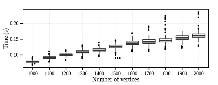
(a)

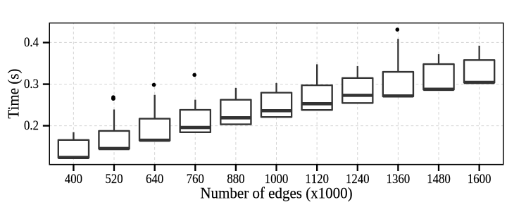
(b)

Figure 2: Running time in seconds of iterations of the system in random networks. (a) The input networks have 400 000 edges and many different numbers of vertices. (b) 2 000 vertices and many different numbers of edges.

Figure 2 depicts the running time of a single iteration of the system varying the number of vertices and edges, respectively. With 10 independent runs, we measure the time for 30 iterations, totalizing 300 samples for each network size. We set $\lambda=1$, two classes, and 5% of labeled vertices. Experiments were run on an Intel® Core™ i7 CPU 860 @ 2.80GHz with 16 GB RAM memory DDR3 @ 1333 MHz. This experiment shows that the system runs in linear time as a function of the number of vertices and edges, which conforms our theoretical analysis.

IV Computer Simulations

To study the stochastic system $\tilde{X}$ and the deterministic version $X$, we present experimental analyses that concern their equivalence. Additionally, we study the meaning of the parameters of our learning model. After that, we evaluate the model performance using both artificial and synthetic datasets. Then, we show the unfolding process and the learning model on synthetic data. Finally, we present the simulation results for a well-known benchmark dataset and for a real application on human activity and handwritten digits recognition.

IV-A Experimental Analysis

In this section, we present an experiment that assesses the equivalence between the unfolding results of both systems with an increasing initial number of particles in system $\tilde{X}$.

The networks used for the analysis are generated by the following model: a complex network $G(\mathbf{y},m,p)$ is constructed given a labeled vector $\mathbf{y}$, a number $m>0$ of edges by vertex, and a weight $p\in[0,1]$ that controls the preferential attachment between vertices of different classes. The resulting network contains $\left\lvert\mathbf{y}\right\rvert$ vertices. For each $v_{i}$, $m$ edges are randomly connected, with replacement. If $y_{i}=y_{j}$, the preferential attachment weight is $1-p$; otherwise, the weight is $p$. The parameter $p$ is proportional to the overlap between classes.

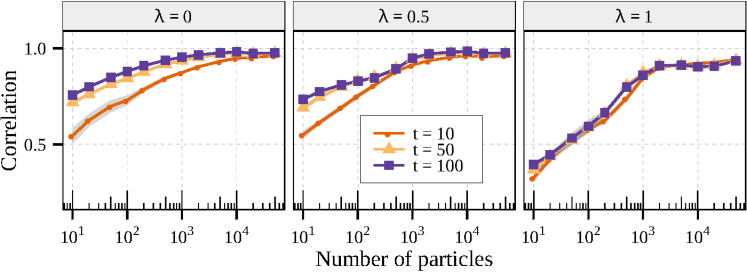
Figure 3: Proportionality simulation. Lines are the correlation measure between the cumulative domination matrices of systems $X$ and $\tilde{X}$, varying the initial number of active particles. Values close to 1 indicate that the cumulative domination matrices of both systems tend to be proportional.

If there exists a positive constant $\kappa$ such that

$$\tilde{\delta}^{c}_{ij}(t)=\kappa\delta^{c}_{ij}(t)\mbox{,}$$

both systems generate the same unfoldings. To assess this proportionality, both systems are simulated in 10 different networks $G(\mathbf{y},3,0.05)$, with $\left\lvert\mathbf{y}\right\rvert=200$ vertices arranged in two classes. The system’s parameter is discretized in $\lambda=\{0,0.5,1\}$. Varying the total number of initial particles, we set $\tilde{n}^{c}_{i}(0)=n^{c}_{i}(0)\sim\operatorname{deg}{v_{i}}$ for all $c\in\{0,\dots,C\}$ and $i\in\{1,\dots,\left\lvert\mathcal{V}\right\rvert\}$.

We consider the correlation between the cumulative domination matrices of systems $X$ and $\tilde{X}$. If the two matrices are proportional, then they must be correlated. Values of correlation close to 1 indicate the cumulative domination matrices are proportional. In Figure 3, the correlation is depicted. As the number of initial particles increases, the correlation approaches 1. This result suggests that both systems generate the same unfolding when the number of initial particles grows to infinity.

IV-B Parameter Analysis

The LCU model has two parameters apart from the network construction. In this section, we discuss their meaning. To do so, the learning model is applied in synthetic datasets whose data items are sampled from a three dimensional knot torus $\mathbf{v}(\theta)$ with parametric curve

$$\begin{split}x(\theta)&=r(\theta)\cos{3\theta},\\ y(\theta)&=r(\theta)\sin{3\theta},\\ z(\theta)&=-\sin{4\theta},\end{split}$$

where $\theta\in[0,2\pi]$ and $r(\theta)=2+\cos{4\theta}$.

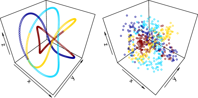
Figure 4: Three dimensional knot torus dataset with 500 samples without noise (left-hand side) and with noise (right-hand side). Colors are the classes.

We sampled 500 data items uniformly along the possible values of $\theta$. We randomly split the data items from 2 to 10 classes so that the samples with adjacent $\theta$ belongs to the same class. We also added to each sample a random noise in each dimension with distribution $\mathcal{N}(0,\sigma)$ with $\sigma=0.25$ and $0.35$. Figure 4 depicts an example of the dataset with 4 classes with and without noise. Since the dataset has a complex form, a small change of parameter value may generate different results. Therefore, it is suitable to study the sensitivity of parameters.

We run the LCU model with parameters $\lambda\in\{0.25,0.5,0.75,1\}$ and $\tau=500$. Finally, 30 unbiased sets of 40 labeled points are employed. The $k$-NN is used for the network construction with $k=\{4,5,\dots,10\}$.

Below, we discuss each parameter of the model.

IV-B1 Discussion about the network construction parameter

In our model, the input network must be simple (between any pair of vertices there must exist at most one edge), unweighted, undirected, and connected. Besides these requirements, two vertices must be connected if their data items are considered similar enough to the particular problem. In our experiments, we use k-NN graph with Euclidean distance since it is proved to approximate the low-dimensional manifold of point set [27]. The smaller the value of $k$, the better are the results.

IV-B2 Discussion about the system parameter

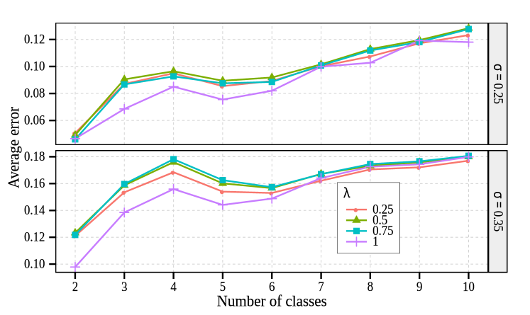
Figure 5: Average error of the proposed model for different numbers of classes in the problem. Colors and shapes indicate the values of parameter $\lambda$.

The LCU system has only one parameter: the competition parameter $\lambda$. This parameter defines the intensity of competition between particles. When $\lambda=0$, particles randomly walk the network, without competition. As $\lambda$ approaches to 1, particles are more likely to compete and, consequently, to be absorbed. Figure 5 depicts the average error of our method with different values of $\lambda$. Based on the figure, our model is not sensitive to $\lambda$. In general, we suggest setting $\lambda=1$ because of better and more consistent classification than other values.

IV-B3 Discussion about the system iteration stopping parameter

The time limit parameter $\tau$ controls when the simulation should stop; it must be at least as large as the diameter of the network. That way, it is guaranteed every edge to be visited by a particle. Since the network diameter is usually a small value, the simulation stops in few iterations.

IV-C Simulations on Artificial Datasets

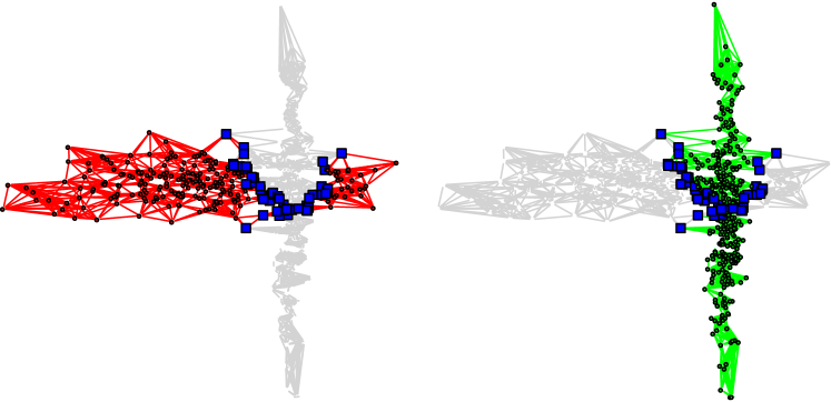
(a)

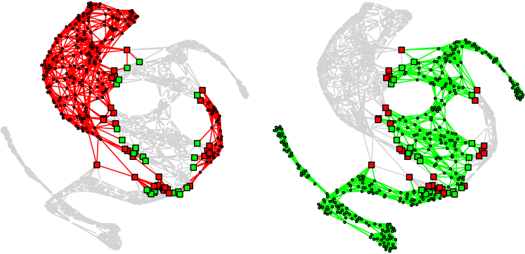
(b)

Figure 6: Unfoldings generated by the proposed system at time $t=100$ on Highleyman dataset. Edges are colored according to the dominating class at the time. Light gray edges stand for edges presented in the original network but not in the unfolding. (a) Vertex position is imposed by the original data points and blue squares represent vertices connected in both unfoldings. (b) Vertex position is not imposed by the original data points and color of the vertices are the result of the classification.

For better understanding the details of the LCU system, in this subsection we illustrate it using two synthetic datasets. Each dataset has a different class distribution—banana shape and Highleyman. (The datasets are generated using the PRTools framework [28].) The banana shape dataset is uniformly distributed along specific shape, and then superimposed on a normal distribution with the standard deviation of 1 along the axes. In Highleyman distribution, two classes are defined by bivariate normal distributions with different parameters. Because the datasets are not in a network representation, we use k-NN graph construction method to transform them into respective network form. In the constructed network, a vertex represents a datum, and it connects to its k nearest neighbors, determined by the Euclidean distance. We set $\lambda=1$ for the simulation.

Firstly, the technique is tested on the Highleyman dataset. Each class has 300 samples, of which 6 are labeled. (We set $k=10$ for the k-NN algorithm.) We can observe that the labeled data points of the green class form a barrier to samples of the red class. The unfoldings $G^{\text{red}}(100)$ and $G^{\text{green}}(100)$ are presented in 6a. In this figure, blue squares represent vertices that are connected by edges of both unfoldings. Besides of the labeled data of green class forming a barrier, the constructed subnetworks are still connected—there is a single component connecting all the vertices of the subnetwork. It is better visualized in 6b. In this figure, the same unfoldings are presented, but the positions of the vertices are not imposed by the original data. Furthermore, colors of vertices in the figure indicate the result of classification. The overlapping data can be identified by the vertices that belong to two or more unfoldings. This result reveals that the competition system in edges provide more information than the competition in vertices since it can identify the overlapping vertices as part of the system, that is, without special treatments or modifications.

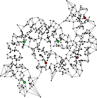
(a)

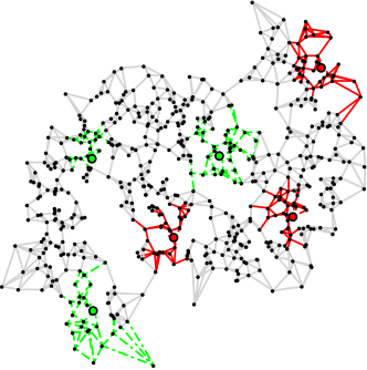
(b)

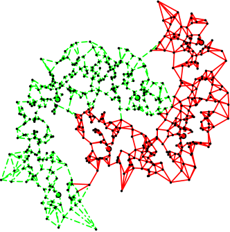
(c)

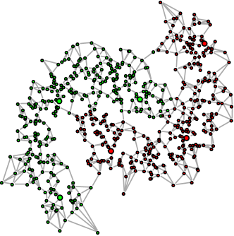
(d)

Figure 7: System evolution on a banana-shaped distribution dataset. Red and green colors represent the two classes. Unlabeled points are black ones; labeled vertices are represented by larger and colored points. Edges are colored according to the dominating class at current iteration, where a light gray point stands for a vertex, which is not dominated yet. (a) The network representation of the dataset at the beginning of the system. (b) and (c) System iteration at time 4 and 20, respectively. (d) The result of the dataset classification.

The last synthetic dataset has 600 samples equally split into two classes. In 7a, the initial state of the system is illustrated, where the dataset is represented by a network. (The network representation is obtained by setting $k=4$ for the k-NN–graph construction.) At this stage, the edges are not dominated by any of the classes. Starting from this state, labeled vertices (sources) generate particles that carry the label of the sources. Though the particles are not shown, 7b and 7c are snapshots of the system evolution—at time 4 and 20—where each edge is colored by its dominating class at that iteration. In these illustrations, a solid red line stands for an edge $(i,j)$ that $\delta^{\text{red}}_{ij}+\delta^{\text{red}}_{ji}>\delta^{\text{green}}_{ij}+\delta^{\text{green}}_{ji}$, while a dashed green line stands for the opposite. When $\delta^{\text{red}}_{ij}+\delta^{\text{red}}_{ji}=\delta^{\text{green}}_{ij}+\delta^{\text{green}}_{ji}$, an edge is drawn in a solid light gray line. As expected, edges close to sources are dominated initially, and farther edges are progressively dominated. At time 20, 7c, every edge has been dominated, and the edge domination does not change anymore. 7d shows dataset classification following the system result. In this example, with 1% of points in the labeled set, the technique can correctly identify the pattern formed by each class. Both results are satisfactory, reinforcing the ability of the technique of learning arbitrary class distributions.

IV-D Simulations on Benchmark Datasets

TABLE II: Test Errors (%) with Standard Deviation and the Best Parameters

10 labeled $k$ $\lambda$ 100 labeled $k$ $\lambda$ g241c 42.90 $\pm$ 4.33 10 0.25 30.03 $\pm$ 2.18 10 0.875 g241n 46.94 $\pm$ 3.93 9 0 36.08 $\pm$ 6.32 9 0 Digit1 4.93 $\pm$ 2.63 5 0.75 1.51 $\pm$ 0.31 6 0.625 USPS 15.65 $\pm$ 3.81 3 1 8.36 $\pm$ 2.92 3 1 COIL 59.96 $\pm$ 6.13 3 0.625 13.73 $\pm$ 2.91 3 0 BCI 47.56 $\pm$ 1.80 9 1 34.68 $\pm$ 2.26 3 0.25 Text 29.71 $\pm$ 3.53 9 0.875 22.41 $\pm$ 1.74 10 0.75

TABLE III: Test Errors (%) with 10 Labeled Training Points

g241c g241d Digit1 USPS COIL BCI Text Avg. Rank 1-NN 47.88 46.72 13.65 16.66 63.36 49.00 38.12 9.3 SVM 47.32 46.66 30.60 20.03 68.86 49.85 45.37 13.0 MVU + 1-NN 47.15 45.56 14.42 23.34 62.62 47.95 45.32 9.3 LEM + 1-NN 44.05 43.22 23.47 19.82 65.91 48.74 39.44 9.1 QC + CMR 39.96 46.55 9.80 13.61 59.63 50.36 40.79 6.9 Discrete Reg. 49.59 49.05 12.64 16.07 63.38 49.51 40.37 10.4 TSVM 24.71 50.08 17.77 25.20 67.50 49.15 31.21 10.0 Cluster–Kernel 48.28 42.05 18.73 19.41 67.32 48.31 42.72 10.1 LDS 28.85 50.63 15.63 17.57 61.90 49.27 27.15 8.0 Laplacian RLS 43.85 45.68 5.44 18.99 54.54 48.97 33.68 5.9 LGC 45.82 44.09 9.89 9.03 63.45 47.09 46.83 6.9 LP 42.61 41.93 11.31 14.83 55.82 46.37 49.53 5.1 LNP 47.82 46.24 8.58 17.87 55.50 47.65 41.06 7.1 Original Particle Competition 41.17 43.51 8.10 15.69 54.18 48.00 34.84 4.0 Labeled Component Unfolding 42.90 46.94 4.93 15.65 59.96 47.56 29.71 4.9

TABLE IV: Test Errors (%) with 100 Labeled Training Points

g241c g241d Digit1 USPS COIL BCI Text Avg. Rank 1-NN 43.93 42.45 3.89 5.81 17.35 48.67 30.11 11.4 SVM 23.11 24.64 5.53 9.75 22.93 34.31 26.45 8.1 MVU + 1-NN 43.01 38.20 2.83 6.50 28.71 47.89 32.83 10.6 LEM + 1-NN 40.28 37.49 6.12 7.64 23.27 44.83 30.77 10.9 QC + CMR 22.05 28.20 3.15 6.36 10.03 46.22 25.71 6.6 Discrete Reg. 43.65 41.65 2.77 4.68 9.61 47.67 24.00 7.1 TSVM 18.46 22.42 6.15 9.77 25.80 33.25 24.52 7.7 Cluster-Kernel 13.49 4.95 3.79 9.68 21.99 35.17 34.28 7.4 LDS 18.04 23.74 3.46 4.96 13.72 43.97 23.15 5.4 Laplacian RLS 24.36 26.46 2.92 4.68 11.92 31.36 23.57 4.4 LGC 41.64 40.08 2.72 3.68 45.55 43.50 56.83 9.3 LP 30.39 29.22 3.05 6.98 11.14 42.69 40.79 8.3 LNP 44.13 38.30 3.27 17.22 11.01 46.22 38.45 11.4 Original Particle Competition 21.41 25.85 3.11 4.82 10.94 41.57 27.92 5.3 Labeled Component Unfolding 30.03 36.08 1.51 8.36 13.73 34.68 22.41 6.0

We compare our model with 14 semi-supervised techniques tested on Chapelle’s benchmark [1]. The benchmark is formed by seven datasets that have 1500 data points, except for BCI that has 400 points. The datasets are described in [1].

For each dataset, 24 distinct, unbiased sets (splits) of labeled points are provided within the benchmark. Half of the splits are formed by 10 labeled points and the other half by 100 labeled points. The author of the benchmark ensured that each split contains at least one data point of each class. The result is the average test error—the proportion of data points incorrectly labeled—over the splits. We compare our results to the ones obtained by the following techniques: 1-Nearest Neighbors (1-NN), Support Vector Machines (SVM), Maximum variance unfolding (MVU + 1-NN), Laplacian eigenmaps (LEM + 1-NN), Quadratic criterion and class mass regularization (QC + CMR), Discrete regularization (Discrete reg.), Transductive support vector machines (TSVM), Cluster kernels (Cluster-Kernel), Low-density separation (LDS), Laplacian regularized least squares (Laplacian RLS), Local and global consistency (LGC), Label propagation (LP), Linear neighborhood propagation (LNP), and Network-Based Stochastic Semisupervised Learning (Vertex Domination), The simulation results are collected from [1], except for LGC, LP, LNP, and Original Particle Competition that are found in [17].

For the simulation of the LCU system, we discretize the interval of the parameter in $\lambda=\left\{0,0.125,\dots,1\right\}$. Also, we vary the k-NN parameter $k\in\left\{1,2,\dots,10\right\}$. We tested every combination of $k$ and $\lambda$. Moreover, we fix $\tau=1000$. In Table II, we present the results with the standard deviation over the splits along with the best combination of parameters that generated the best accuracy result.

The test error comparison for 10 labeled points are shown in Table III; comparison for 100 labeled points are in Table IV. Apart from each dataset, the last column is the average performance rank of a technique over the datasets. A ranking arranges the methods under comparison by test error rate in ascending order. For a single dataset, we assign rank 1 for the method with the lowest average test error on that dataset, then rank 2 for the method with the second lowest test error, and so on. The average ranking is the average value of the rankings of the method on all the datasets. The smaller the ranking score, the better the method has performed.

From the average rank column, the LCU technique is not the best ranked, but it is in the best group of techniques in both 10 labeled and 100 labeled cases.

We statistically compare the results presented in Tables III and IV. For all tests we set a significance level of $5\%$. First, we use a test based on the average rank of each method to evaluate the null hypothesis that all the techniques are equivalent. With the Friedman test [29], there is statistically significant difference between the rank of the techniques

Since the Friedman test result reports statistical significance, we use the Wilcoxon signed-rank test [29]. In this pairwise difference test, we test for the null hypothesis that the first technique has greater or equal error results than the second. If rejected at a 5% significance level, then we say the first technique is superior to the second. By analyzing results for 10 and 100 labeled points together, we conclude that our technique is superior to 1-NN, LEM + 1-NN, and MVU + 1-NN. Examining separately, for 10 labeled points, our method is also superior to discrete regularization, cluster kernel, and SVM. For 100 labeled points, it is also superior to LNP and LGC; whereas Laplacian RLS is superior to ours.

IV-E Simulations on Human Activity Dataset

TABLE V: Performance Comparison in the Human Activity Recognition Using Smartphones Dataset

Labeled Component Unfolding SVM 5% labeled 10% labeled 20% labeled $\approx$70% labeled [30] Precision Recall F Score Precision Recall F Score Precision Recall F Score Precision Recall F Score WK .984 $\pm$ .013 .941 $\pm$ .030 .962 $\pm$ .016 .992 $\pm$ .004 .985 $\pm$ .011 .989 $\pm$ .006 .994 $\pm$ .002 .997 $\pm$ .001 .995 $\pm$ .001 .957 .992 .974 WU .981 $\pm$ .009 .935 $\pm$ .026 .957 $\pm$ .015 .988 $\pm$ .008 .961 $\pm$ .013 .974 $\pm$ .008 .991 $\pm$ .003 .981 $\pm$ .006 .986 $\pm$ .004 .980 .958 .969 WD .987 $\pm$ .017 .901 $\pm$ .016 .942 $\pm$ .011 .994 $\pm$ .008 .918 $\pm$ .011 .955 $\pm$ .007 .998 $\pm$ .001 .945 $\pm$ .008 .971 $\pm$ .004 .988 .976 .982 ST .864 $\pm$ .034 .698 $\pm$ .049 .770 $\pm$ .022 .883 $\pm$ .015 .743 $\pm$ .039 .806 $\pm$ .020 .905 $\pm$ .014 .814 $\pm$ .015 .857 $\pm$ .006 .969 .880 .922 SD .840 $\pm$ .024 .842 $\pm$ .053 .839 $\pm$ .017 .870 $\pm$ .023 .844 $\pm$ .022 .856 $\pm$ .006 .896 $\pm$ .013 .872 $\pm$ .021 .884 $\pm$ .009 .901 .974 .936 LD .996 $\pm$ .002 .999 $\pm$ .000 .998 $\pm$ .001 .997 $\pm$ .001 .999 $\pm$ .000 .998 $\pm$ .000 .997 $\pm$ .001 .999 $\pm$ .000 .998 $\pm$ .000 1.000 1.000 1.000

The Human Activity Recognition Using Smartphones [30] dataset comprises of 10299 data samples. Each sample matches 561 features extracted from motion sensors attached to a person during a time window. Each person performed six activities which are target labels in the dataset—walking (WK), walking upstairs (WU), walking downstairs (WD), sitting (ST), standing (SD), and laying down (LD).

We use k-NN with $k=7$ for the dataset network representation once it is the smallest value that generates a connected network. The parameters are fixed in $\lambda=1$ and $\tau=1000$. We compare our results with the ones published in [30], splitting the problem into six binary classification tasks.

Table V summarises the results. For our technique, we provide the precision, recall and F Score using 5%, 10%, and 20% of labeled samples. We average the results of 10 independent labeled set for each configuration. We also provide the original results from [30] using SVM with approximately 70% of labeled samples. Our technique performs as well as SVM using far fewer labeled samples and using the suggested parameter set. Such a feature is quite attractive because it may represent a big saving in money or efforts when involving manually data labeling in semi-supervised learning.

IV-F Simulations on MNIST Dataset

TABLE VI: Test Errors (%) in the MNIST Dataset

Method	100 labeled	1000 labeled
LCU	$10.62\pm 1.91$	$6.31\pm 0.46$
TSVM* [23]	$16.81$	$5.65$
Embed NN* [31]	$16.86$	$8.52$
Embed CNN* [31]	$7.75$	$3.82$

• ^* The comparison is biased since the results from [23, 31] rely on a single and unique labeled set. See text for more details.

The MNIST dataset comprises 70,000 examples of handwritten digits. All digits have been size-normalized and centered in a fixed-size image. In a supervised learning setting, this dataset is split into two sets: 60,000 examples for training and 10,000 for testing.

To adapt the dataset to a semi-supervised learning problem, we use a setting similar to [23, 31]: the labeled input data items are selected from the training set, and the unlabeled ones from the test set. Although we do not use a validation set, [23] and [31] use an additional set of at least 1,000 labeled samples for parameter tuning.

The network representation is obtained from the images without preprocessing. We use the Euclidean distance between items and $k=3$ to construct the k-NN network. Similarly to the previous experiment, the value of $k$ is the smallest value that generates a connected network. The parameters are fixed in $\lambda=0.9$ and $\tau=500$.

Table VI compares the error rate of our method to other semi-supervised techniques. To the best of our knowledge, we could not find many papers with experiments under the same semi-supervised settings for the MNIST dataset. Due to such available results in the literature, we sought to carry our experiments with the input as similar as possible to the compared results. However, a single sampling with as less as 1,000 labeled samples out of a set of 60,000 images most probably results in a biased accuracy result, we opt to average results from 15 labeled sets for each parameter setting.

Our model performs well even without preprocessing and validation set. This result indicates that besides the simplicity of the constructed network, our learning system can obtain enough knowledge from data.

V Conclusion

We have presented a transductive semi-supervised learning technique based on a vertex-edge dynamical system on complex networks. First, the input data is mapped into a network. Then, the proposed Labeled Component Unfolding (LCU) system runs on this network. At this stage, particles compete for edges in the network. When a particle passes through an edge, it increases its class dominance over the edge while decreasing other classes’ dominance. Three dynamics—walking, absorption and production—provide a biologically inspired scenario of competition and cooperation. Then, labels are assigned according to the dominant class over the edges. As a result, the system unfolds the original network by grouping edges dominated by the same class. Finally, we employ the unfoldings to classify unlabeled data. Furthermore, rigorous studies have been done on the novel LCU system.

The deterministic system implementation brings advantages over its stochastic counterpart. The time complexity of the deterministic one does not depend on the number of particles, so we are benefited from better results when considering a continuously varying number of initial particles. Besides, the LCU system allows a stable transductive semi-supervised learning technique with a subquadratic order of complexity. Computer simulations show the proposed technique achieves a good classification accuracy and it is suitable for situations where a small number of labeled samples are available. Another interesting feature of the proposed model is that it directly provides the overlapping information of each vertex or a subset of vertices.

As future works, we would like to investigate the mathematical property of the LCU system on directed or weighted networks. Besides of this, it is interesting to improve the runtime further via network sampling methods or estimation methods. In this way, the model will be suitable to be applied to process large enough datasets or streaming data. Another interesting research is to treat the labels on edges instead of nodes in a semi-supervised learning environment.

References

- [1] O. Chapelle, B. Schölkopf, and A. Zien, Eds., Semi-Supervised Learning. Cambridge, MA: MIT Press, 2006.
- [2] X. Zhu and A. B. Goldberg, Introduction to Semi-Supervised Learning, 3rd ed. Morgan and Claypool Publishers, 2009.
- [3] K. Nigam, A. K. McCallum, S. Thrun, and T. Mitchell, “Text classification from labeled and unlabeled documents using EM,” Machine Learning, vol. 39, no. 2-3, pp. 103–134, 2000.
- [4] M. Loog and A. C. Jensen, “Semi-Supervised Nearest Mean Classification Through a Constrained Log-Likelihood,” IEEE Trans. Neural Netw. Learn. Syst., vol. 26, no. 5, pp. 995–1006, 2015.
- [5] K. Wagstaff, C. Cardie, S. Rogers, and S. Schroedl, “Constrained k-means clustering with background knowledge,” in Proc. of the 18th International Conference on Machine Learning, 2001, pp. 577–584.
- [6] Z.-H. Zhou and M. Li, “Tri-training: exploiting unlabeled data using three classifiers,” IEEE Trans. Knowl. Data Eng., vol. 17, no. 11, pp. 1529–1541, 2005.
- [7] V. N. Vapnik, Statitical learning theory. New York, NY: Wiley, 1998.
- [8] T. C. Silva and L. Zhao, “Semi-supervised learning guided by the modularity measure in complex networks,” Neurocomputing, vol. 78, no. 1, pp. 30–37, 2012.
- [9] L. Cheng and S. J. Pan, “Semi-supervised Domain Adaptation on Manifolds,” IEEE Trans. Neural Netw. Learn. Syst., vol. 25, no. 12, pp. 2240–2249, 2014.
- [10] K. Zhang, L. Lan, J. T. Kwok, S. Vucetic, and B. Parvin, “Scaling Up Graph-Based Semisupervised Learning via Prototype Vector Machines,” IEEE Trans. Neural Netw. Learn. Syst., vol. 26, no. 3, pp. 444–457, 2015.
- [11] M. Belkin, P. Niyogi, and V. Sindhwani, “Manifold regularization: A geometric framework for learning from labeled and unlabeled examples,” J. Mach. Learn. Res., vol. 7, pp. 2399–2434, 2006.
- [12] M. Newman, A.-L. Barabási, and D. J. Watts, The Structure and Dynamics of Networks: Princeton Studies in Complexity. Princeton University Press, 2006.
- [13] M. E. J. Newman, Networks: An Introduction, 1st ed. New York, NY: Oxford University Press, 2010.
- [14] T. C. Silva and L. Zhao, Machine Learning in Complex Networks, 1st ed. Springer, 2016.
- [15] X. Zhu, A. B. Goldberg, and T. Khot, “Some new directions in graph-based semi-supervised learning,” Proc. of the EEE International Conference on Multimedia and Expo, pp. 1504–1507, 2009.
- [16] M. G. Quiles, L. Zhao, R. L. Alonso, and R. A. F. Romero, “Particle competition for complex network community detection,” Chaos, vol. 18, no. 3, p. 033107, 2008.
- [17] T. C. Silva and L. Zhao, “Network-based stochastic semisupervised learning,” IEEE Trans. Neural Netw. Learn. Syst., vol. 23, no. 3, pp. 451–66, 2012.
- [18] ——, “Network-based stochastic semisupervised learning,” IEEE Trans. Neural Netw. Learn. Syst., vol. 23, no. 3, pp. 451–466, 2012.
- [19] ——, “Detecting and preventing error propagation via competitive learning,” Neural Networks, vol. 41, pp. 70–84, 2013.
- [20] J. Jensen, “Sur les fonctions convexes et les inégalités entre les valeurs moyennes,” Acta Mathematica, vol. 30, no. 1, pp. 175–193, 1906.
- [21] J. L. Bentley, “Multidimensional binary search trees used for associative searching,” Commun. ACM, vol. 18, no. 9, pp. 509–517, 1975.
- [22] D. Zhou, O. Bousquet, T. N. Lal, J. Weston, and B. Schölkopf, “Learning with local and global consistency,” in Advances in Neural Information Processing Systems 16, S. Thrun, L. Saul, and B. Schölkopf, Eds. MIT Press, 2004, pp. 321–328.
- [23] R. Collobert, F. Sinz, J. Weston, and L. Bottou, “Large Scale Transductive SVMs,” Journal of Machine Learning Research, vol. 7, no. 7, pp. 1687–1712, 2006.
- [24] B. Wang, Z. Tu, and J. K. Tsotsos, “Dynamic label propagation for semi-supervised multi-class multi-label classification,” Proc. of the IEEE International Conference on Computer Vision, pp. 425–432, 2013.
- [25] X. Zhu and Z. Ghahramani, “Learning from labeled and unlabeled data with label propagation,” School Comput Sci Carnegie Mellon Univ Pittsburgh PA Tech Rep, vol. 54, no. CMU-CALD-02-107, pp. 1–19, 2002.
- [26] Y. M. Zhang, K. Huang, G. G. Geng, and C. L. Liu, “MTC: A Fast and Robust Graph-Based Transductive Learning Method,” IEEE Trans Neural Netw Learn Syst, vol. 26, no. 9, pp. 1979–1991, 2014.
- [27] J. B. Tenenbaum, V. de Silva, and J. C. Langford, “A global geometric framework for nonlinear dimensionality reduction,” Science, vol. 290, no. 5500, p. 2319, 2000.
- [28] R. Duin, P. Juszczak, P. Paclík, E. Pekalska, D. de Ridder, D. Tax, and S. Verzakov, “PR-Tools4.1, a matlab toolbox for pattern recognition,” 2007.
- [29] M. Hollander and D. A. Wolfe, Nonparametric Statistical Methods, 2nd ed. Wiley-Interscience, 1999.
- [30] D. Anguita, A. Ghio, L. Oneto, X. Parra, and J. L. Reyes-Ortiz, “A Public Domain Dataset for Human Activity Recognition Using Smartphones,” in 21th European Symposium on Artificial Neural Networks, Computational Intelligence and Machine Learning, ESANN 2013, 2013.
- [31] J. Weston, F. Ratle, H. Mobahi, and R. Collobert, “Deep learning via semi-supervised embedding,” in In Neural Networks: Tricks of the Trade. Springer, 2012, pp. 639–655.