Read networks and k-laminar graphs

Abstract

In this paper we introduce k-laminar graphs a new class of graphs which extends the idea of Asteroidal triple free graphs. Indeed a graph is k-laminar if it admits a diametral path that is k-dominating. This bio-inspired class of graphs was motivated by a biological application dealing with sequence similarity networks of reads (called hereafter read networks for short). We briefly develop the context of the biological application in which this graph class appeared and then we consider the relationships of this new graph class among known graph classes and then we study its recognition problem. For the recognition of k-laminar graphs, we develop polynomial algorithms when k is fixed. For k=1, our algorithm improves a Deogun and Krastch’s algorithm (1999). We finish by an NP-completeness result when k is unbounded.

Keywords: diameter, asteroidal triple, diametral path graphs, k-dominating paths, k-laminar graphs, (meta)genomic sequences, reads, read networks.

1 Introduction and biological motivation

Roughly speaking a k-laminar graph has a spine and all others vertices are closed to the spine (a more formal definition will be given in the next section). The definition of this graph class was motivated by its appearance in reads similarity networks of genomics or metagenomics data [4] see Figure 1. In sequence similarity networks, vertices are biological sequences (either DNA or protein sequences) and two vertices are adjacent if the corresponding sequences are similar, meaning that the pair shows a high enough BLAST score [2] and matches over more than 90% of the longest sequence. Here, sequences come from a metagenomic project and are usually called reads. Basically, reads are raw sequences that come off a sequencing machine, they are random DNA fragments, roughly 300 characters long, coming from the various microbial genomes that are found in a given environment. In our multidisciplinary approach [3] we wonder if two species of lizards can be distinguished by the analysis of read networks sequenced from the microbial DNA (microbiome) present in their gastro enteric tract. These networks are useful to biologists because, in addition to allowing the visualization of the genetic diversity that is found in the microbes of a given environment, they offer an alternative to more classical approaches, like the building of contigs, where one tries to rebuild the original genomic sequences of each organism out of the fragments, after a step of binning. The step of binning is a process which clusters contigs or reads, generally based on their composition, and tries to assign them to Operational Taxonomic Units (OTUs - which is the most commonly used microbial diversity unit)[16]. Sequence similarity networks are indeed a relaxation of de Bruijn graphs [7], which are commonly used to build contigs, since they are undirected and, more importantly, since two sequences are adjacent if they show a high enough, but not necessarily exact, similarity. In particular, they allow for the quantification of the genetic diversity of an ensemble of reads. For example of such networks, see Figure 1.

When a subset of reads covers a contiguous part of a genome (or parts of the genomes which have the same origin (common ancestor) also called homologous parts), they assemble into a k-laminar graph in sequence similarity networks, thus defining a singular genomic context (e.g. a suite of genes) on which biologists can measure the genetic diversity of the community. However, some genetic sequences, like repeats or transposases, can be found in more than one genomic context (i.e. when copies of the same transposase are inserted in multiple distinct locations of a genome), effectively linking together k-laminar graphs in sequence similarity networks. Building contigs out of sequences from such connected components is an especially difficult task.

To sum it up, sequence similarity networks of reads are thus composed of k-laminar parts, corresponding to singular regions of the genomes of a given environment, joined together by groups of vertices corresponding to repetitions in the genomes of a given environment. Identifying k-laminar parts in such networks, and eventually achieving a k-laminar decomposition, is thus of major interest to biologists.

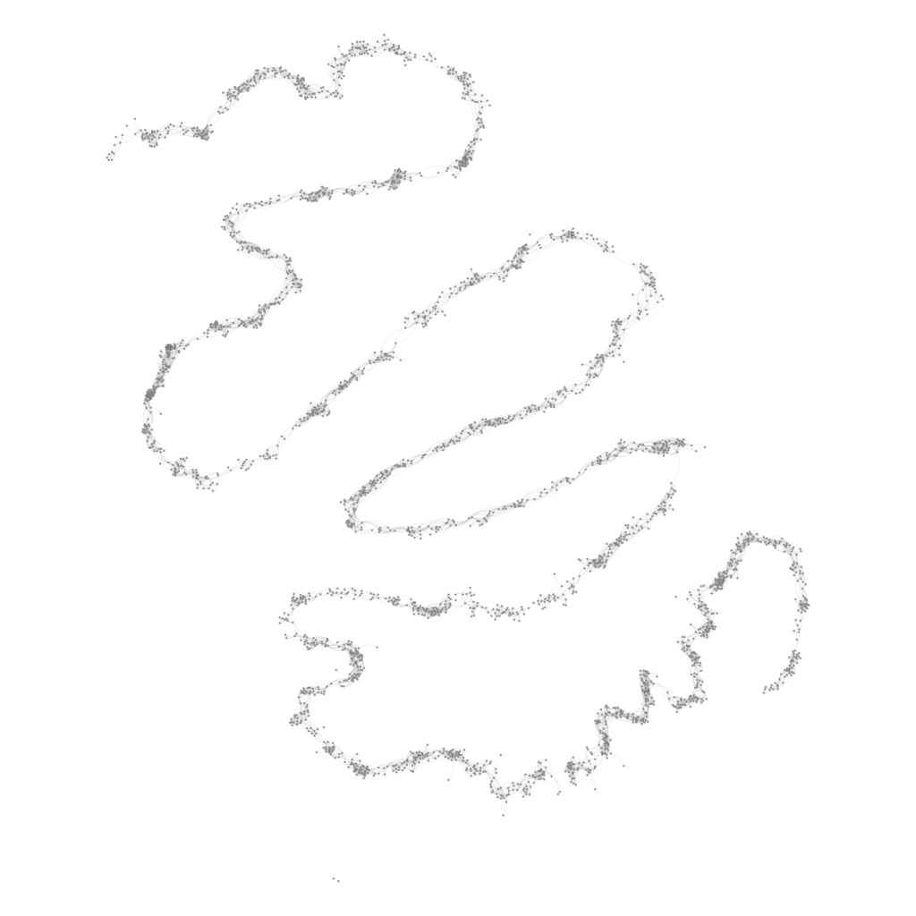
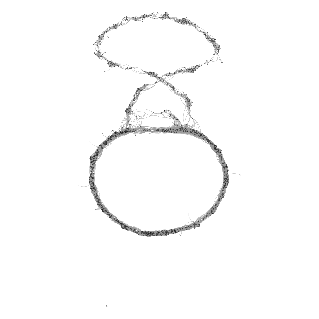
Figure 1: Two read graphs: the left one is a 4-laminar graph, the right one contains big cycles but can be decomposed into 4-laminars parts. Data used here comes from our project [3].

2 k-laminar graphs

The graphs considered here are finite, loopless and undirected. For a connected graph $G$, with vertex set $V(G)$ and edge set $E(G)$, we denote by $d(x,y)$ for $x,y\in V(G)$ the distance between two vertices, i.e., the length of a shortest path joining $x$ to $y$ in $G$. We will use also the notion of eccentricity of a vertex $x\in V(G)$: $ecc(x)=max_{y\neq x,y\in V(G)}d(x,y)$ and so the diameter is $diam(G)=max_{x\in V(G)}ecc(x)$, similarly the radius is defined as $radius(G)=min_{x\in V(G)}ecc(x)$. Furthermore let us denote by $MaxEcc(G)$ the set of all vertices of maximum eccentricity. When there is no ambiguity for a graph $G$ we will denote by $n,m$ respectively $|V(G)|,|E(G)|$.

We extend this notion to the distance of vertex to a path, namely $d(x,\mu)$, for some path $\mu$, is the smallest distance from $x$ to some vertex on $\mu$. $N(x)$ will be the standard neighborhood of a vertex and we use also the notation $N[x]=N(x)\cup\{x\}$ for the closed neighborhood.

Similarly $N^{k}(x)$ the k-neighborhood, i.e. the vertices with distance equal to k from $x$ or more formally $N^{k}(x):=\{y\ |\ d(x,y)=k\}$. We denote by $N^{k}[x]$ all vertices with distance less or equal to k, i.e. $N^{k}[x]:=\{y\ |\ d(x,y)\leq k\}$ called the closed k-neighborhood. When $G$ is connected, the maximum length of a path is called the diameter of $G$ and denoted by $diam(G)$.

In this section we recall some standard definitions on graphs and introduce the notion of laminar graphs and the practical motivations of such a definition.

Definition 1.

An asteroidal triple (AT) is a triple of vertices such that each pair is joined by a path that avoids the neighborhood of the third.

An AT-free graph is a graph that does not contain any AT. Intuitively if a graph does not contain any AT, then it cannot ”expand” in more than 2 directions. The following definition of laminar graphs introduced here, is to generalize this intuitive notion of linearity.

Definition 2.

A path $\mu$ of a graph $G$ is a diametral path if the length of $\mu$ is equal to $diam(G)$. Furthermore for every fixed integer $k$, a path $\mu$ in a graph $G$ is called a $k$-dominating path if $\forall x\in V(G)$ we have $d(x,\mu)\leq k$.

Definition 3.

A graph $G$ is called $k$-laminar (resp. strongly $k$-laminar) if $G$ has a $k$-dominating diametral path (resp. if every diametral path is $k$-dominating).

Proposition 4.

[8] AT-free graphs are 1-laminar.

Proof.

Corneil, Olariu and Stewart proved that AT-free graphs contain a dominating pair that achieves the diameter. Hence, AT-free graphs are 1-laminar. ∎

Definition 5.

A comparability graph is a graph $G$ whose edge set $E(G)$ can be transitively oriented. A cocomparability graph is simply the complement of a comparability graph.

It is well known that cocomparability graphs are AT-free [9]. Therefore also cocomparability graphs and interval graphs are 1-laminar.

Figure 2: $\mu=[a,b,c,d,h]$ is a dominating diametral path of $G_{1}$, and $(a,f,h)$ is an AT.

As shown by the graph $G_{1}$ of Figure 2, not all 1-laminar graphs are AT-free graphs. Thus AT-free graphs $\subsetneq$ 1-laminar. Furthermore AT-free are not always strongly 1-laminar as can be seen with the graph $G_{2}$ of Figure 3. To complete the picture, the class of AT-free graphs overlaps the class of 1-strongly laminar as can be seen with the graph $G_{3}$ of Figure 4.

Figure 3: $G_{2}$ is AT-free but $\mu=[a,b,c,d,e]$ is a non dominating diametral path of $G_{2}$.

Figure 4: $G_{3}$ is not AT-free, (g, i, d) is an AT, but $G_{3}$ is 1-strongly laminar.

The smallest k such that a graph is k-laminar is called the laminar index of $G$ and denoted by $Laminar(G)$. This invariant is well defined since obviously $Laminar(G)\leq diam(G)$ and furthermore if a center of the graph belongs to a diametral path: $Laminar(G)\leq radius(G)$. This paper is devoted to the study of (strongly) k-laminar graphs, their structure but also the existence of polynomial recognition algorithms. Since it is well known that a graph may have an exponential number of diametral paths (see for example the graph in Figure 6), at first glance we can only state that the recognition problem of strongly k-laminar paths is in co-NP. In [10], Deogun and Kratsch introduced a very similar graph class, namely the diametral path graphs.

Definition 6.

[10] A graph G is called a diametral path graph if every connected induced subgraph H of G has a dominating diametral path or equivalently $H$ is a 1-laminar graph using definition 3.

It is not hard to see that all diametral path graphs are 1-laminar. But 1-laminar graphs strictly contain diametral path graphs, as can be seen with the graph $G_{1}\setminus\{d\}$ which is no 1-laminar. Therefore $G_{1}\in$ 1-laminar graphs $\setminus$ diametral path graphs.

Using a polynomial time algorithm [10] for testing if a graph has a dominating diametral path, we know that the recognition of 1-laminar graphs is polynomial.

Moreover Deogun and Kratsch were able to prove that diametral path graphs that are trees or chordal graphs have simple forbidden subgraphs (polytime-recognizable). But to our knowledge it is still an open question whether diametral path graphs can be recognized in polynomial time.

Figure 5: Relationships among the main graph classes considered so far, including that AT-free $\subset$ Diametral Path Graphs as first noticed in [13].

The remaining part of the paper is organized as follows:

In section 3 we show that the recognition of strongly laminar graphs is polynomial, such as the recognition of k-laminar graphs when k is fixed. To this aim we improve an algorithm from [10] to recognize 1-laminar graphs and we generalize it for every fixed k.

In section 4 we present strong evidence that it is intractable to find the laminar index. In fact we present a reduction which proves that recognizing if a graph $G$ is $k$-laminar is NP-complete, for a given range of $k$ values in $O(\sqrt{|V(G)|})$.

3 Polynomial algorithms

The main contribution of this section is that we present a polynomial recognition algorithms for any fixed k for k-laminar (resp. strongly k-laminar) graphs. Let us begin with the strongly case.

3.1 Strongly k-laminar graphs

First we need an easy lemma.

Lemma 7.

Let $x\in MaxEcc(G)$ and $H$ be an induced subgraph of $G$ containing $x$. If $ecc_{H}(x)=diam(G)$ then there exists a shortest path $\mu=[x,y]$ in $H$ and $G$ of size $diam(G)$.

Proof.

We notice that $ecc_{G}(x)\leq ecc_{H}(x)$. In case of equality it yields that there exists a path $\mu=[x,y]$ in $H$ of length $diam(G)$. $\mu$ is still a shortest path with no shortcut in $G$, unless $x\in MaxEcc(G)$. ∎

Theorem 8.

The recognition of strongly k-laminar graphs can be done in $O(|MaxEcc(G)|nm)$ bounded by $O(n^{2}m)$ for every fixed $k$.

Proof.

If a graph is not strongly k-laminar then there exists some diametral path that does not pass through the k-neighborhood of some vertex $x$. It suffices therefore to verify that every diametral path passes through $N^{k}[x]$ $\forall x\in V$. This can easily be done by recalculating the distance matrix in $G\setminus N^{k}[x]$ for every $x$. We know that $diam(G\setminus N^{k}[x])\geq diam(G)$.

If for some vertex $x$ $d_{G\setminus N^{k}[x]}(a,b)=d_{G}(a,b)=diam(G)$, using lemma 7 we know there exsit some path $\mu$ in $G$ which is a diametral path that does not pass through $N^{k}[x]$ and therefore the strongly laminar condition is not satisfied.

We need for every vertex $x$ to compute $G^{\prime}=G\setminus N^{k}[x]$ which can be done $O(|V(G|+|E(G)|)$ using a BFS. But then we must compute the eccentricity of all $MaxEcc(G)$ vertices in $G^{\prime}$ which can be done in a naive way by processing $|MaxEcc(G)|$ BFS’s in $O(|V(G^{\prime})|.|E(G^{\prime})|)$.

Therefore for each $k$ this can be done in $O(|MaxEcc(G)|nm)$, i.e., in $O(n^{2}m)$. ∎

As an immediate consequence:

Corollary 9.

The computation of the smallest k for which a graph $G$ is k-strongly laminar is polynomial.

Proof.

Since $1\leq k\leq n-1$ and we can use a dichotomic process of the above algorithm, which yields a complexity of $O(log(n)n^{2}m)$. ∎

3.2 1-laminar graphs

Let us now describe an improved variation of the $O(n^{3}m)$ Deogun and Kratsch’s algorithm [10], searching for the existence of a dominating diametral path in $O(n^{2}m)$.

As a preprocessing, we can compute $ecc(x)$ for every vertex $x$ of $G$. Afterwards $\forall s\in MaxEcc(G)$, we process a BFS and let us denote by $T_{s}$ the associated BFS-tree. $L_{i}$ represent the different layers of the BFS-tree, i.e. by convention $L_{0}=\{s\}$ and $L_{i}$ is equal to the i-th neighborhood of $s$. Then $\forall v\in V(G)$, let us denote by $Level_{s}(v)$ its level in $T_{s}$. We can also preprocess in linear time : $\forall v\in V(G)$ and $\forall i$ such that $Level_{s}(v)$-$1\leq i\leq Level_{s}(v)+1$ we compute $N_{i}(v)=N(v)\cap L_{i}$.

Then we can use for every vertex $s\in MaxEcc(G)$ the following modified BFS, which is in fact a partial BFS since only the vertices that can be part of a dominating diametral path are explored.

Dominating-Diameter(G,s):

Data: a graph $G=(V,E)$ and a start vertex $s\in MaxEcc(G)$;

Result: YES / NO $G$ has a dominating diametral path starting at $s$;

Mark FEASIBLE all edges adjacent to $s$. Initialize Queue to $N(s)$;

while $Queue\neq\emptyset$ do

      dequeue $v$ from beginning of Queue;

       $h\leftarrow Level_{s}(v)$;

      

      for $\forall u\in N_{h-1}(v)$ with $uv$ marked FEASIBLE do

            

            $A(v)\leftarrow N_{h}(v)\cup N_{h}(u)$;

             if $h=diam(G)$ then

                  if $L_{h}=A(v)$ then

                         YES a dominating diametral path from $s$ to $v$ has been found STOP

                   end if

                  

             end if

            for  $\forall w\in N_{h+1}(v)$ do

                  

                  if $L_{h}$=$A(v)\cup N_{h}(w)$ then

                        

                        Mark $vw$ as FEASIBLE;

                         if $w$ is not already in Queue then

                               enqueue $w$ to the end of Queue

                         end if

                        

                   end if

                  

             end for

            

       end for

      

end while

NO $G$ has no dominating diametral path starting at $s$;

Algorithm 1 A modified Breadth First Search

Theorem 10.

Algorithm Dominating-Diameter(G,s) computes if a graph $G$ admits a dominating diametral path starting from $s$ in $O(nm)$.

Proof.

Any diametral path must go sequentially through the all the layers of $H_{i}$. Furthermore using the BFS-tree structure any edge $xy\in V(G)$ satisfies $|Level_{s}(x)-Level_{s}(y)|\leq 1$.

In order to prove the modified BFS algorithm we need to prove that for every vertex $s$ of maximal eccentricity it is enough to check that the following easy invariant s:

Invariant 11.

For all i, $1\leq i\leq Diam(G)$, and for every $v\in L_{i}(s)$ If $v\in Queue$, then there exists a path from $s$ to $v$ in $G$, that dominates the first $i-1$ layers. Moreover all these dominating paths reach $v$ with an edge marked FEASIBLE.

Complexity analysis: The preprocessing time, i.e., computing all eccentricities can be done in a naive way by processing $n$ Breadth First searches (BFS) in $O(nm)$.

Let us consider a BFS search starting at some $s\in MaxEcc(G)$ and its BFS numbering $\tau$ (the visiting ordering of the vertices during the BFS), one can easily sort all the neighborhood lists of all the vertices according to $\tau$ in linear time. Then for every vertex $x\in L_{h}$, $N_{h-1}(x),N_{h}(x)$ and $N_{h+1}(x)$ can be extracted from $N(x)$ in $O(1)$. Therefore for each BFS before using the modified BFS, the preprocessing requires $O(n+m)$. The structure of the modified BFS, i.e., the while loop, is a partial BFS visiting only vertices that can still belong to a dominating path. Let us now consider the inside instructions.

For every edge $uv$ the test $L_{h}$=$A(v)\cup N_{h}(w)$ can be done by computing $A(v)\cap N_{h}(w)$ in $O(|A(v)|+|N_{h}(w)|)$ since they are encoded as sorted lists and then comparing the sizes $|A(v)\cap N_{h}(w)|$ and $|L_{h}|$ in $O(1)$.

For every vertex $v\in L_{h}$, in the whole : $N_{h}(v)$ is used at most $|N_{h-1}(v)|+|N_{h+1}(v)|$ times.

Therefore for all $v$ it is bounded by $\Sigma_{v}|N_{h}(v)|(|N_{h-1}(v)|+|N_{h+1}(v)|)$. Bounding $|N_{h-1}(v)|+|N_{h+1}(v)|$ by $n$ we obtain: $n.\Sigma_{v}d(v)\in O(n.m)$ Therefore the overall time complexity of this algorithm is $O(nm)$. ∎

Corollary 12.

The recognition of 1-laminar graphs can be done in $O(|MaxEcc(G)|.nm)$ bounded by $O(n^{2}m)$.

Proof.

To recognize if a graph is 1-laminar, it is enough to process for every $s\in MaxEcc(G)$ the algorithm Dominating-Diameter(G,s). Including the preprocessing and the computation of all eccentricities in $G$ in $O(nm)$, the overall time complexity is $O(|MaxEcc(G)|.nm)$ bounded by $O(n^{2}m)$. ∎

This algorithm can be easily adapted to compute a 1-dominating diametral path and generalized for every fixed integer $k$, and this yields :

Theorem 13.

The recognition of k-laminar graphs can be done in $O(n^{2k+1})$.

For a proof the reader is referred to the Appendix.

4 NP-completeness

In this section we give a reduction from 3SAT to the recognition of $k$-laminar graphs. It is therefore NP-hard to compute $Laminar(G)$. The reader is encouraged to look at figure 6 for an better understanding of the reduction. In this section $n$ denotes the number of variables in a satisfiability formula and $N$ the number of vertices in a graph. Capital letters are used to denote vertices and small letters to denote variables.

Given a 3SAT formula $\phi$ made up with $m$ clauses $C_{j}$, $1\leq j\leq m$, on $n$ boolean variables $x_{i}$ $1\leq i\leq n$.

We construct a graph $G(\phi)$ and we will prove that: $G(\phi)$ is $(\frac{n}{2}+1)$-laminar iff $\phi$ is satisfiable.

Let us first detail the construction of $G(\phi)$. For each literal $x_{i}$ (resp. $\overline{x_{i}}$) we associate a vertex $X_{i}$ (resp. $\overline{X_{i}}$). We put an edge between a variable and its negation. Moreover we connect the vertices $X_{i}$ and $\overline{X_{i}}$ with $X_{i-1},\overline{X_{i-1}},X_{i+1},\overline{X_{i+1}}$ if existent. We add a pending chain $V_{1},\dots V_{n}$ to $X_{1}$ and $\overline{X_{1}}$. The same is done symmetrically with a pending chain $V_{n+1},\dots V_{2n}$ attached to $X_{n}$ and $\overline{X_{n}}$. Up to now we have $2^{n}$ shortest paths of length $3n+2$ going from $V_{1}$ to $V_{2n}$. Now for every clause $C_{i}$, $1\leq j\leq m$, we add a vertex $C_{i}$. Every $C_{i}$ is connected by a chain of length $\frac{n}{2}+1$ to every vertex associated to a litteral that appears in the clause $C_{i}$. Note that here for sake of simplicity $n$ is supposed to be even, otherwise we would add a dummy variable.

Suppose for now that the diametral path starts and ends from the end vertices of the two chains respectively ($V_{1}$ and $V_{2n})$. Such a diametral path will never pass through $X_{i}$ and $\overline{X_{i}}$ because it would either need to use an edge $X_{i}\overline{X_{i}}$ or do some detour which would mean that the length of the path is greater than the diameter $3n+2$.

The graph $G(\phi)$ contains exactly $4n+m_{\phi}(\frac{n}{2}+1)=|V(G)|$ vertices, where $m_{\phi}$ is the total number of variables in the clauses $C_{j}$.

Lemma 14.

$diam(G(\phi))=3n+2$

Proof.

For any pair of clauses : $C_{j},C_{j^{\prime}}$ , $d(C_{j},C_{j^{\prime}})\leq 2(\frac{n}{2}+1)+n\leq 3n$

Furthermore: Let $p$ (resp. $q$) be the minimum (resp. maximum) index of a literal in $C_{j}$.

Then $ecc(C_{j})=max\{n-p+n+1,n+1+q\}=max\{2n-p+1,n+q+1\}\leq 2n+1.$

We already have seen that : $ecc(V_{1})\leq 3n+2$, using a path going only through the $X_{i}$’s up to $V_{2n}$. Moreover no $C_{j}$ can provide a shortcut to this path. Thus $ecc(V_{1})=3n+2=ecc(V_{2n})$

∎

Figure 6: An example of graph $G(\phi)$

Theorem 15.

$G(\phi)$ is a $(\frac{n}{2}+1)$-laminar graph iff $\phi$ is satisfiable.

Proof.

Suppose $\phi$ is satisfiable and let $\mathbb{A}$ be some satisfying truth assignment of the variables. Consider a path $\mu$ from $V_{1}$ to $V_{2n}$ forced to visit the vertex $X_{i}$ if the variable is set to true in $\mathbb{A}$ and $\overline{X_{i}}$ otherwise.

$\mu$ is obviously a diametral path. Since $\mathbb{A}$ is a truth assigment every clause $C_{j}$ of $\phi$ has a true literal which belongs to $\mu$ and therefore $d(C_{j},\mu)\leq\frac{n}{2}+1$. All other vertices either belongs to $\mu$ are at distance 1. Therefore $\mu$ is ($\frac{n}{2}+1$)-dominating diametral path.

Conversely, suppose $G(\phi)$ is $(\frac{n}{2}+1)$-laminar, hence using Lemma 14 there exists a diametral path $\mu$ of length $3n+2$ such that a every vertex is at distance $\frac{n}{2}+1$ from $\mu$. As explained above $X_{i}$ and $\overline{X_{i}}$ can not be both on a diametral path. We set the variable $x_{i}$ to be true if $\mu$ passes through the vertex $X_{i}$ to false otherwise. Every clause $C_{j}$ must be satisfied because there is at least one variable vertex $X_{j}$ at distance $\frac{n}{2}+1$ from it. Therefore this ($\frac{n}{2}+1$)-dominating diametral path provides a truth assignment for $\phi$. ∎

It is obvious that the transformation can be computed in polynomial time. Let us consider the following decision problem :

Name: Laminarity

Data: A graph $G$ and $k$ an integer such that $k\in[\frac{\sqrt{|V(G)|}}{4},\frac{\sqrt{|V(G)|}}{2}]$

Question: Is $G$ $k$-laminar ?

Corollary 16.

Laminarity is an NP-complete problem.

Proof.

If we consider the 3SAT NP-complete variant in which every variable occurs at most 3 times [14]. The relationship between the number of variables $n$ of such an instance and its number of clauses $m$ is :

$2n\leq m_{\phi}\leq 3n$ where $m_{\phi}$ denotes the total number of occurences of variables in clauses. This inequalities just say that each variable has 2 or 3 occurences in the clauses, since we can get rid of the cases where a variable occurs only in one clause.

Considering the first inequalities we deduce:

$4n+2n(\frac{n}{2}+1)\leq|V(G)|\leq 4n+3n(\frac{n}{2}+1)$, which gives : $n^{2}+6n\leq|V(G)|\leq 3\frac{n^{2}}{2}+7n$.

Replacing $n$ by $2k-1$ we obtain : $4k^{2}+8k-5\leq|V(G)|\leq 12k^{2}+2K-4$.

Therefore : $4k^{2}\leq|V(G)|\leq 16k^{2}$

If we consider the range $[\frac{\sqrt{|V(G)|}}{4},\frac{\sqrt{|V(G)|}}{2}]$ for $k$, using the construction described above we can encode all instances of a NP-complete variant of 3SAT. ∎

5 Conclusion and perspectives

It would be interesting to improve the running time for the recognition of k-laminar graphs (especially for 1-laminar ones). But it should be noticed that for graphs having a constant number of extremal vertices (i.e., $|MaxEcc(G)|$ is bounded by this constant) then the complexity of the algorithms proposed here in theorems 8,10 goes down to $O(nm)$ which could be optimal, see [5, 1]. In particular when dealing with read networks their laminar parts seem to have a bounded number of extremal vertices.

One of the few theoretical results on clustering for restricted graph classes is presented in [12] and proposes an approximation algorithm for 1-laminar graphs. Therefore we think that these bio-inspired k-laminar graphs are worth to be studied further. As for example, searching for diameter computations in linear time using a constant number of BFSs as in [6] and may have other applications not only in bioinformatics.

Perhaps the k-laminar class of graphs is too large to capture all properties of read networks. The good notion could be k-diametral path graphs with its recursive definition for all induced subgraphs. Unfortunately there is no polynomial recognition algorithm for this class. A good algorithmic compromise would be to add some connectivity requirements, i.e., k-laminar and h-connected. It would be interesting to develop a robust decomposition method of read networks into their k-laminar parts. In other words we want to find a skeleton of a read network that captures most of its biological properties. Such a decomposition could provide an interesting alternative process to analyze the biodiversity of read networks.

Acknowledgements: The authors wish to thank Anthony Herrel for many discussions on the project and for having selected the lizards on which this study is based.

6 Appendix

6.1 k-laminar recognition algorithm

We first notice that every graph $G$ is trivially $diam(G)$-laminar, and let us now generalize the previous recognition algorithm 1 to any fixed integer $k$ such that : $k<diam(G)$.

Theorem 17.

For every fixed $k\geq 2$ such that $k<diam(G)$, the algorithm k-Dominating-Diameter(G,s) finds a k-dominating diametral path starting form $s$ if some exists in $O(n^{2k})$.

Proof.

To generalize Dominating-Diameter(G,s) algorithm, we will proceed similarly from a given vertex $s\in MaxEcc(G)$, by considering all the paths of length $k$ starting at $s$ and then make them grow layer by layer keeping only those which are potential extendable to a k-dominating diametral path.

We keep the same preprocessing as for the recognition of 1-laminar graphs, namely: we can compute $ecc(x)$ for every vertex $x$ of $G$. Afterwards $\forall s\in MaxEcc(G)$, we process a BFS and let us denote by $T_{s}$ the associated BFS-tree. $L_{i}$ represent the different layers of the BFS-tree, i.e. by convention $L_{0}=\{s\}$ and $L_{i}$ is equal to the i-th neighborhood of $s$. Then $\forall v\in V(G)$, let us denote by $Level_{s}(v)$ its level in $T_{s}$. We can also preprocess in the same time : $\forall v\in V(G)$ and $\forall i$ such that $Level_{s}(v)$-$k\leq i\leq Level_{s}(v)+k$ we compute $N^{k}_{i}(v)=N^{k}(v)\cap L_{i}$. Since $k$ is fixed, the sets $N^{k}_{i}(v)$ can be computed in $O(nm)$ also.

k-Dominating-Diameter(G,s):

Data: a graph $G=(V,E)$ and a start vertex $s\in MaxEcc(G)$, an integer $k\geq 2$;

Result: YES / NO $G$ has a k-dominating diametral path starting at $s$;

Initialisations:

Initialize a queue Queue with all different pairs $(v,P)$ such that $P$ is a path of length $k$ starting at $s$ in the BFS-tree, and $v$ its last vertex. This list is supposed to be lexicographically ordered accordingly to the layer orderings.

while $Queue\neq\emptyset$ do

      dequeue $(v,P)$ from beginning of Queue;

      

      $p\leftarrow Level_{s}(v)$ ;

       $q\leftarrow p-k+2$ ;

       $A(v)\leftarrow\bigcup_{u\in P,q-k+1\leq Level_{s}(u)\leq p}N^{k}_{q}(u)$;

      

      if $p=diam(G)$ then

            if $\forall i$, $q\leq i\leq p$, $L_{i}=\bigcup_{u\in P,i-k+1\leq Level_{s}(u)\leq i+k}N^{k}_{i}(u)$ then

                   YES ”a k-dominating diametral path from $s$ to $v$ has been found”STOP

             end if

            

       end if

      for  $\forall x\in N_{p+1}(v)$ do

            

            if $L_{q}$=$A(v)\cup N^{k}_{q}(x)$ then

                  

                  $P^{\prime}\leftarrow P+x$ ;

                   enqueue $(x,P^{\prime})$ to the end of Queue ;

                  

             end if

            

       end for

      

end while

NO ”$G$ has no k-dominating diametral path starting at $s$”;

Algorithm 2

Invariant: If the pair $(v,P)$ with $P=[s,\dots v]$ belongs to Queue, and if $p=Level_{s}(v)$ then $P$ a path k-dominating the first $p-k+1$ layers.

This invariant is clearly satisfied with the initializations of Queue. Then During the While loop a new pair $(v,P)$ is only inserted if it satisfies this property.

Complexity Analysis: The initialisation step may costs $O(n^{k})$ since we could have $\prod_{i=1}^{h}|L_{i}|$ different pairs $(v,P)$. The queue data structure forces the vertices to be visited in a breadth first way, giving an $O(n+m)$ to the managment of the while loop. During this while loop:

For every vertex $v$ the set $A(v)$ is used at most $|N_{p+1}(v)|$ times, so in the whole it is bounded by $O(nm)$. But to compute the sets $A(v)$ we have to maintain paths of length 2k. Unfortunately there could be $n^{2k}$ such paths. This yields a polynomial algorithm in $O(n^{2k})$.

∎

Corollary 18.

k-laminar graphs can be recognized in $O(|MaxEcc(G)|.n^{2k})$ or $O(n^{2k+1})$.

Proof.

First we have to compute all eccentricites in $G$ in $O(nm)$ and then it is enough to repeat this Algorithm 2 for every $x\in MaxEcc(G)$, this provides an algorithm running $O(|MaxEcc(G)|.n^{2k})$.

∎

References

- [1] A. Abdoud, V.V. Williams, J. Wang, Approximation and Fixed parameter subquadratic algorithms Radius and Diameter, in Proceedings of the twenty-seventh annual ACM-SIAM symposium on Discrete Algorithms, p. 377-391, SIAM, 2016.
- [2] S. F. Altschul, W. Gish, W. Miller, E. W. Myers, D. J. Lipman, Basic local alignment search tool, Journal of molecular biology, vol. 3, p. 403-410, 2015.
- [3] E. Bapteste, M. Habib, A. Herrel, P. Lopez, C. Vigliotti, Projet Evolézards, Défi ENVIROMICS, Mission Interdisciplinarité CNRS, 2014.
- [4] E. Boon, S. Halary, E. Bapteste, M. Hijri, Studying genome heterogeneity within the arbuscular mycorrhizal fungal cytoplasm, Genome Biol Evol. Jan 7;7(2): 505-521, 2015.
- [5] M. Borassi, P. Crescenzi, M. Habib, Into the Square - On the Complexity of Quadratic-Time Solvable Problems, CoRR, abs/1407.4972, 2014.
- [6] M. Borassi, P. Crescenzi, M. Habib, W. A. Kosters, A. Marino, F. W. Takes, Fast diameter and radius BFS-based computation in (weakly connected) real-world graphs: With an application to the six degrees of separation games, Theor. Comput. Sci., Vol 586, p. 59-80, 2015.
- [7] Phillip E C Compeau, Pavel A Pevzner , Glenn Tesler, How to apply de Bruijn graphs to genome assembly, Nature Biotechnology 29, p. 987-991, 2011
- [8] D.G. Corneil, S. Olariu, L. Stewart, Asteroidal triple-free graphs, SIAM J. Discrete Math., Vol 10, No. 3, p. 399-430, 1997.
- [9] M.C. Golumbic, C.L. Monma, W.T. Trotter, Tolerance graphs, Disc. Applied Math. 9, p. 157-170, 1997.
- [10] J.S. Deogun, D. Kratsch, Diametral Path Graphs, Graph Theoretic Concepts in CS, p. 344-357, 1999.
- [11] J.S. Deogun, D. Kratsch, Dominating Pair Graphs, SIAM J. Discrete Math., Vol. 15, No. 3, p. 353-366, 2002.
- [12] J.S. Deogun, D. Kratsch, G. Steiner, An approximation algorithm for clustering graphs with dominating diametral path, Information Processing Leters, 61, p. 121-127,1997.
- [13] D. Kratsch, The structure of graphs and the design of efficient algorithms, Habilitation Thesis, Friedrich-Schiller-Universität, Jena, 1995.
- [14] C. H. Papadimitriou, Computational Complexity, 1994, Addison-Welsey.
- [15] Y. Peng, Henry C. Leung, S.M. Yu, F.Y. L. Chin, IBDA-UD a de novo assembler for single-cell and metagenomic sequencing data with highly uneven depth, Bioinformatics, Volume 28, Issue 11, p. 1420-1428, 2012.
- [16] J. H. Saw, A. Spang, K. Zaremba-Niedzwiedzka, L. Juzokaite, J. A. Dodsworth, S. K. Murugapiran, D. R. Colman, C. Takacs-Vesbach, B. P. Hedlund, L. Guy and T. J. Ettema, Exploring microbial dark matter to resolve the deep archaeal ancestry of eukaryotes. Philos Trans R Soc Lond B Biol Sci 370(1678): 20140328 (2015).