Time-Dependent Density Functional Theory Beyond Kohn-Sham Slater Determinants

Abstract

When running time-dependent density functional theory (TDDFT) calculations for real-time simulations of non-equilibrium dynamics, the user has a choice of initial Kohn-Sham state, and typically a Slater determinant is used. We explore the impact of this choice on the exchange-correlation potential when the physical system begins in a 50:50 superposition of the ground and first-excited state of the system. We investigate the possibility of judiciously choosing a Kohn-Sham initial state that minimizes errors when adiabatic functionals are used. We find that if the Kohn-Sham state is chosen to have a configuration matching the one that dominates the interacting state, this can be achieved for a finite time duration for some but not all such choices. When the Kohn-Sham system does not begin in a Slater determinant, we further argue that the conventional splitting of the exchange-correlation potential into exchange and correlation parts has limited value, and instead propose a decomposition into a “single-particle” contribution that we denote $v_{\scriptscriptstyle\rm XC}^{\scriptscriptstyle\rm S}$, and a remainder. The single-particle contribution can be readily computed as an explicit orbital-functional, reduces to exchange in the Slater determinant case, and offers an alternative to the adiabatic approximation as a starting point for TDDFT approximations.

I Introduction and Motivation

Time-Dependent Density Functional Theory (TDDFT) Ullrich (2011); Marques et al. (2012); Runge and Gross (1984) is increasingly being used beyond linear response applications, to study fully non-equilibrium dynamics of electronic systems in real-time. Although TDDFT has had much success in the linear response regime in calculations of spectra, it is perhaps a more enticing tool for real-time dynamics when the system is driven far from its ground-state, because of the computational challenges in describing such dynamics for more than two electrons with alternative wavefunction-based methods. TDDFT presents an attractive possibility due to its system-size scaling, arising from its description of the dynamics in terms of a non-interacting system of electrons evolving in a single-particle potential. In practise the many-body effects hidden in this potential, termed the exchange-correlation (xc) potential, must be approximated. The Runge-Gross and the van Leeuwen van Leeuwen (1999) theorems reassure us that there exists an exact xc potential for which the time-dependent one-body density of the interacting system is exactly predicted. It is therefore of much interest what the features of this exact xc potential look like in order to develop approximations that build in these features.

The exact xc potential at a given time $t$ is known to depend on the density not just at time $t$ but also on its history, and it additionally depends on the initial wavefunction of the physical system $\Psi(0)$, as well as the choice of initial Kohn-Sham wavefunction $\Phi(0)$: $v_{\scriptscriptstyle\rm XC}[n;\Psi(0),\Phi(0)]$. Typically however, in real-time TDDFT simulations adiabatic approximations are used which depend only on the instantaneous density: $v_{\scriptscriptstyle\rm XC}^{A}[n;\Psi(0),\Phi(0)]=v_{\scriptscriptstyle\rm XC}^{\rm g.s.}[n(t)]$. That is, they insert the instantaneous density into a ground-state approximation. This approximation has provided useful results for the interpretation and prediction of electron-dynamics in a range of situations, including photovoltaic design Rozzi et al. (2013), high-harmonic generation in molecules Penka Fowe and Bandrauk (2011), coherent phonon generation Shinohara et al. (2012), ultrafast demagnetization of solids Elliott et al. (2016). However, in some cases there are complete failures, e.g. Refs. Raghunathan and Nest (2011, 2012); Habenicht et al. (2014), and studies on model systems have revealed that there are large non-adiabatic features in the exact xc potential that are missing in the approximations. These include step and peak features that evolve in time Ramsden and Godby (2012); Hodgson et al. (2013, 2014); Elliott et al. (2012); Fuks et al. (2013); Luo et al. (2014, 2013). These dynamical features appear generically when the system has been pushed out of equilibrium, whether or not there is an external field present. They have been analyzed in terms of the local acceleration across the system Elliott et al. (2012) and in terms of a decomposition into kinetic and interaction xc components Luo et al. (2014). The latter generalizes a concept from the ground-state that was pioneered by Evert Jan Baerends and his group Buijse et al. (1989); Gritsenko et al. (1994, 1996); Gritsenko and Baerends (1996), which had provided valuable insight into analyzing the structure of the ground-state xc potential in atoms and molecules.

In this paper, we will focus on the initial-state dependence of these non-adiabatic features, and on the xc potential in general. The initial interacting state $\Psi(0)$ is given by the problem at hand, but one has a choice of initial Kohn-Sham state $\Phi(0)$ in which to begin the non-interacting Kohn-Sham evolution. The only restriction is that $\Phi(0)$ must have the same initial density and first time-derivative of the density as that of $\Psi(0)$. Almost always, an initial single Slater determinant (SSD) of orbitals is chosen, even when the initial interacting state is far from an SSD. For example, in simulating photo-induced dynamics, where the true state is a singlet single excitation of the molecule, a typical practise is simply to raise one electron from the Kohn-Sham HOMO and place it in a virtual orbital; spin-adaptation is done after the dynamics is run. The true initial state on the other hand requires at least two Slater determinants for a minimal description. The exact xc potential for model systems with different choices of initial Kohn-Sham states can vary significantly, and so the question arises: Is there an optimal choice of Kohn-Sham initial state, for which the exact xc potential has minimal non-adiabatic features, such that propagating this state using an adiabatic functional yields the smallest errors?

Preliminary investigations considered initial stationary excited states, and suggested the “best” Kohn-Sham initial state when using an adiabatic approximation has a configuration similar to the initial interacting state Elliott and Maitra (2012). That work was limited to studying the exact xc potentials compared with the adiabatic ones at the initial time, while time-propagation was considered only using common adiabatic approximations, since to find the exact xc potential for a Kohn-Sham state that has more than one occupied orbital is very demanding. Refs. Nielsen et al. (2013, 2014), on the other hand, used the recently introduced global fixed-point iteration method Ruggenthaler and van Leeuwen (2011); Ruggenthaler et al. (2012); Penz and Ruggenthaler (2011); Nielsen et al. (2013); Ruggenthaler et al. (2015); Nielsen et al. (2014) to find the exact xc potential in time for different choices of Kohn-Sham initial state for a given density of two particles interacting via a cosine interaction on a ring.

In this paper we go further, returning to the more physical soft-Coulomb interaction used in Ref. Elliott and Maitra (2012), and investigate the exact xc potential for different choices of Kohn-Sham initial states as a function of time using the iteration procedure of Ref. Nielsen et al. (2013, 2014), for field-free dynamics of a superposition state. We compare with the adiabatically-exact (AE) approximation, which is defined as the exact ground-state xc potential evaluated on the exact density Thiele et al. (2008). This is the best possible adiabatic approximation, and is what the intensive efforts in building increasingly sophisticated approximations for ground-state problems strive towards. We find that although the AE approximation is a better approximation for some choices of Kohn-Sham initial state than others, at least for short times, it is not particularly good for any of them for the strongly non-equilibrium dynamics considered here. We expect therefore the AE propagation to be inaccurate. Instead we introduce a different starting point for TDDFT approximations, based on the time-dependent xc hole of the Kohn-Sham wavefunction. This is motivated by the decomposition of Refs. Ruggenthaler and Bauer (2009); Luo et al. (2014), where the Kohn-Sham wavefunction is used to evaluate the interaction term, and yields an explicit orbital functional. We denote this approximation $v_{\scriptscriptstyle\rm XC}^{\scriptscriptstyle\rm S}$, and it contains some non-adiabatic contributions. The exact xc potential is decomposed as $v_{\scriptscriptstyle\rm XC}=v_{\scriptscriptstyle\rm XC}^{\scriptscriptstyle\rm S}+v_{\scriptscriptstyle\rm XC}^{\scriptscriptstyle\rm NS}$, which we propose as the basis for a new approximation strategy which is particularly promising in the case of initial Kohn-Sham states that resemble the initial interacting state, going beyond the usual Kohn-Sham SSD.

II Model System and Different Initial States

The soft-Coulomb interaction Javanainen et al. (1988) has been used extensively in strong-field physics as well as in density-functional theory as it captures much of the physics of real atoms and molecules. The particular Hamiltonian we choose represents a model of the Helium atom prepared in a superposition state. We place two soft-Coulomb interacting electrons in a one-dimensional (1D) soft-Coulomb well (atomic units are used throughout),

$$\hat{H}=\sum_{i=1,2}\left(-\frac{1}{2}\frac{d^{2}}{dx_{i}^{2}}-\frac{2}{\sqrt{x_{i}^{2}+1}}\right)+\frac{1}{\sqrt{|x_{1}-x_{2}|^{2}+1}},$$ (1)

prepared in a 50:50 superposition state of the ground and first-excited singlet state of the interacting system, that is then allowed to evolve freely:

$$\Psi(0)=\frac{1}{\sqrt{2}}\left(\Psi_{0}+\Psi_{1}\right),$$ (2)

where $\Psi_{i}=\Psi_{i}(x_{1},x_{2})$ denote the many-body eigenstates of Hamiltonian (1). The dynamics of the density,

$$n(x,t)=2\int dx^{\prime}|\Psi(x,x^{\prime},t)|^{2}\;,$$ (3)

therefore is a periodic sloshing inside the well, with period $2\pi/(E_{1}-E_{0})=11.788$ a.u. We place the system in a box with infinite walls at $x=\pm L/2=7.5$au, giving zero boundary conditions at $\pm L/2$.

II.1 Different choices of initial Kohn-Sham state

We will study the features of the exact xc potential evaluated at this many-body density when different initial Kohn-Sham states are propagated. First, we define

$$\Phi^{(a)}(0)\equiv\frac{1}{\sqrt{1+a^{2}}}\left(\Phi_{0}+a\Phi_{1}\right)$$ (4)

where

$$\Phi_{0}(x_{1},x_{2})=\Phi^{\rm g.s.}=\phi_{0}^{(a)}(x_{1})\phi_{0}^{(a)}(x_{2})$$ (5)

is the non-interacting ground-state of an ($(a)$-dependent) potential and

$$\Phi_{1}(x_{1},x_{2})=\frac{1}{\sqrt{2}}\left(\phi_{0}^{(a)}(x_{1})\phi_{1}^{(a)}(x_{2})+\phi_{1}^{(a)}(x_{1})\phi_{0}^{(a)}(x_{2})\right)$$ (6)

is the first non-interacting singlet single-excitation of that same potential; $\phi_{0}^{(a)}$ and $\phi_{1}^{(a)}$ are the ground and first-excited orbitals of this potential. Clearly the orbitals and potential depend on the parameter $a$, but such that in all cases $\Phi^{(a)}$ reproduces the same initial density and zero current-density as $\Psi(0)$. We will consider different values for $a$, focussing particularly on:

(i) $\Phi(0)=\Phi^{a=0}$. By requiring the initial density and zero current-density match, we immediately obtain $\phi_{0}^{a=0}=\sqrt{n(x,0)/2}$. This is the conventional choice for TDDFT, an SSD. The exact xc potential in this case, $v_{\scriptscriptstyle\rm XC}[n;\Psi(0),\Phi^{a=0}]$ was studied before for this problem in Refs. Elliott et al. (2012); Luo et al. (2014), and large non-adiabatic step and peak features were observed. They are missing in all adiabatic approximations, and even the exact ground-state xc potential i.e. the AE, looks completely different than the exact. A point of the present paper is to explore whether a different choice of initial Kohn-Sham state can reduce these non-adiabatic features.

(ii) $\Phi(0)=\Phi^{a=1}$, which is a non-interacting analog of the form of the true interacting state. Unlike in case (i), there are many possible pairs of orbitals with this form that reproduce a given density and current-density. The reason is that here we do not consider a ground state and hence do not have the Hohenberg-Kohn uniqueness theorem. Our choice here has a relatively large overlap with the interacting state. See also (iii).

(iii) $\Phi(0)=\widetilde{\Phi}^{a=1}$, has the same form of (ii) but with a different pair of orbitals that are eigenstates of quite a different potential, and with a significantly smaller overlap with the true interacting state.

(iv) $\Phi(0)=\Psi(0)$; the initial Kohn-Sham state is chosen identical to the initial interacting state.

In addition to the four states above, we will also show some results for other $a$ but will not study these situations in so much detail.

In Figure 1, we plot the orbitals of these states, and the potentials in which they are eigenstates. While in the case $a=0$ we know the form of the initial Kohn-Sham orbitals and the corresponding Kohn-Sham potential analytically as a density-functional,

$$v_{\scriptscriptstyle\rm S}^{\rm g.s.}[n](x)=\frac{1}{2}\frac{\partial_{x}^{2}\sqrt{n(x)}}{\sqrt{n(x)}},$$ (7)

for $a\neq 0$ we use an iterative method along the lines of Ref. van Leeuwen and Baerends (1994). An exposition of the method is given in appendix A.

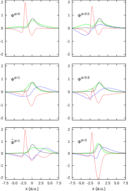
Figure 1: Non-interacting potential $v$ (red, solid) for which the $\phi_{0}^{(a)}$ (green, long-dashed) and $\phi_{1}^{(a)}$ (blue, short-dashed) that form the initial KS wavefunction $\Phi^{(a)}(0)$, Eq. (4), are eigenstates. In black, dotted, the initial density $n(x,0)$ is plotted.

Any of these states may be used to initiate a time-dependent Kohn-Sham calculation. If the exact xc potential was used, then propagating using $h^{\scriptscriptstyle\rm S}$,

$$h^{\scriptscriptstyle\rm S}=\sum_{i=1,2}\Big{(} -\frac{1}{2}\frac{d^{2}}{dx_{i}^{2}}-\frac{2}{\sqrt{x_{i}^{2}+1}}+v_{\scriptscriptstyle\rm H}[n](x_{i},t)\Big{)}$$ (8)

$$+v_{\scriptscriptstyle\rm XC}[n;\Psi(0),\Phi(0)](x_{i},t)\Big{)}$$

where $v_{\scriptscriptstyle\rm H}[n](x_{i},t)=\int dx^{\prime}n(x^{\prime},t)/\sqrt{(x_{i}-x^{\prime})^{2}+1}$ and $v_{\scriptscriptstyle\rm XC}$ is different for each choice of initial Kohn-Sham state, then the exact time evolving density of the interacting system Eq. (3) is reproduced. In practise, the exact xc potential is unknown. How closely the approximate functionals, in particular, adiabatic ones that depend only on the instantaneous density, approximate the exact xc potential gives an indication of how accurately the approximate functional reproduces the density. Since adiabatic functionals neglect all initial-state dependence (and dependence on the density’s history), then when evaluated on a given density, it gives the same potential for any of the choices of the Kohn-Sham initial state, unlike the exact xc potential.

In the next section we explain how we find the exact xc potential for a given choice of initial Kohn-Sham state.

III Finding the Exact xc Potential via the Global Fixed-Point Method

To find the exact xc potential for a given physical density evolution is generally a non-trivial task. One must effectively find a one-body potential in which non-interacting electrons evolve yielding the exact physical density of the interacting system at each instant in time; even whether, or when, such a potential exists is not a completely closed question Ruggenthaler et al. (2015). The non-adiabatic step and peak features that have been highlighted in Refs. Elliott et al. (2012); Fuks et al. (2013); Luo et al. (2014) involve a particularly simple case: two electrons in 1D, where the Kohn-Sham initial state is taken to be a doubly-occupied orbital (as in (i) in the previous section), that evolves as $\phi(x,t)=|\phi(x,t)|e^{i\alpha(x,t)}$. The amplitude of this orbital is fixed from requiring the instantaneous density is reproduced, $n(x,t)=2|\phi(x,t)|^{2}$, while its phase follows from use of the continuity equation in 1D: $\partial_{t}n(x,t)=-\partial_{x}j$ where $j$ is the one-body current, $j(x,t)=n(x,t)\partial_{x}\alpha(x,t)$. Thus the exact Kohn-Sham orbital can be readily reconstructed from knowledge of $n(x,t)$, and the Kohn-Sham equation inverted to find the Kohn-Sham potential; subtracting the external and Hartree potentials yields the exact xc potential. Despite the simple procedure (see also Ruggenthaler et al. (2013) for the periodic case), the resulting xc potential displays a wealth of interesting non-adiabatic features, absent in ground-state potentials. For more electrons and more dimensions, a numerical iteration scheme is required instead, and has been performed for quasiparticle propagation in a model one-dimensional 20-electron nano-wire Ramsden and Godby (2012) and for two electrons along a two-dimensional ringNielsen et al. (2014). Sometimes lattice models can soothe the computational cost Schmitteckert et al. (2013); Fuks and Maitra (2014); Karlsson et al. (2011); Verdozzi et al. (2011).

III.1 Global Fixed Point Iteration Method

Even for two electrons in 1D, the inversion to explore different possibilities for Kohn-Sham initial states becomes non-trivial. As soon as more than one Kohn-Sham orbital is involved, one must guarantee not only that the time-dependent density is reproduced at each instant in time from the sum-square of these orbitals, but also that each orbital is evolving consistently in the same one-body potential. In this work, we utilize the global fixed point iteration method recently introduced in Refs. Ruggenthaler and van Leeuwen (2011); Ruggenthaler et al. (2012); Penz and Ruggenthaler (2011); Nielsen et al. (2013, 2014); Ruggenthaler et al. (2015) to find the exact Kohn-Sham potential for the different choices of initial Kohn-Sham states. This method uses the fundamental equation of TDDFT, which is employed in the founding papers Runge and Gross (1984); van Leeuwen (1999) and describes the divergence of the local forces (here in 1D for simplicity)

$$\partial_{t}^{2}n(x,t)=\partial_{x}\left(n(x,t)\partial_{x}v_{\scriptscriptstyle\rm S}(x,t)\right)-\partial_{x}Q_{\scriptscriptstyle\rm S}(x,t),$$ (9)

where $Q_{\scriptscriptstyle\rm S}(x,t)=\langle\Phi(t)|\hat{Q}_{\scriptscriptstyle\rm S}(x)\Phi(t)\rangle$ is the internal force density of the Kohn-Sham system due to the momentum-stress forces $\hat{Q}_{\scriptscriptstyle\rm S}(x)=-i[\hat{j}(x),{\hat{T}}]$ Tokatly (2005). In the case of the physical, interacting, system the internal force density also contains a contribution from the interaction forces, i.e., $\hat{Q}(x)=-i[\hat{j}(x),{\hat{T}}+\hat{W}]$ Tokatly (2005). If we prescribe the density $n(x,t)$ and fix an initial Kohn-Sham state $\Phi(0)$, then Eq. (9) becomes a non-linear equation for the external potential $v_{\scriptscriptstyle\rm S}[n;\Phi(0)](x,t)$ that reproduces $n(x,t)$. The solution to this equation can then be found by an iteration procedure of the form

$$-\partial_{x}\left(n(x,t)\partial_{x}v_{\scriptscriptstyle\rm S}^{k+1}(x,t)\right) = \partial^{2}_{t}(n^{k}(x,t)-n(x,t))$$

$$- \partial_{x}\left(n^{k}(x,t)\partial_{x}v_{\scriptscriptstyle\rm S}^{k}(x,t)\right),$$

where we used Eq. (9) to express $\partial_{x}Q_{\scriptscriptstyle\rm S}^{k}(x,t)$ in terms of $v_{\scriptscriptstyle\rm S}^{k}(x,t)$ and $n^{k}(x,t)$, the density produced by propagating $\Phi(0)$ with $v_{\scriptscriptstyle\rm S}^{k}(x,t)$. In the case of zero boundary conditions on the wave functions we then solve for $v_{\scriptscriptstyle\rm S}^{k+1}(x,t)$ by imposing that the potential needs to be even about the boundaries $x=\pm L/2$ Nielsen et al. (2013, 2014); Ruggenthaler et al. (2015). We then iterate until convergence. [The actual numerical implementation uses a slightly different form of Eq. (III.1) that also contains the current density and iterates for each individual time step. In this way numerical errors can be suppressed. For a detailed discussion of the algorithm the reader is refered to Nielsen et al. (2014)]. This then allows us to determine the xc potential from

$$v_{\scriptscriptstyle\rm XC}[n;\Psi(0),\Phi(0)]=v_{\scriptscriptstyle\rm S}[n;\Phi(0)]-v-v_{\scriptscriptstyle\rm H}[n],$$ (11)

where $v=-2/\sqrt{x^{2}+1}$ is explicitly given by the problem at hand. (As a functional $v=v[n;\Psi(0)]$, the potential that generates the prescribed density from $\Psi(0)$ in the interacting system, but we do not directly utilize this functional dependence.)

IV Results: The exact time-dependent xc potential

Ref. Elliott et al. (2012) showed that for the Kohn-Sham non-interacting system to exactly reproduce the density dynamics of the 50:50 superposition state when an SSD is used, the exact xc potential develops large step and peak like features that are completely missed by any adiabatic approximation, even the “best” adiabatic approximation, the AE. Can these features be reduced if the Kohn-Sham system is allowed to go beyond an SSD?

In Figures 2 and 3 we show the exact xc potential $v_{\scriptscriptstyle\rm XC}[n;\Psi(0),\Phi(0)](x,t)$ at various times for the different choices of Kohn-Sham initial state detailed in Section II. The SSD case, $\Phi^{a=0}$ is shown in both plots as reference. The evolution of the xc potential for longer times is shown in Figures 4, 5, and 6, for the KS initial state choices $a=0$, $a=1$ and $\Phi(0)=\Psi(0)$ respectively.

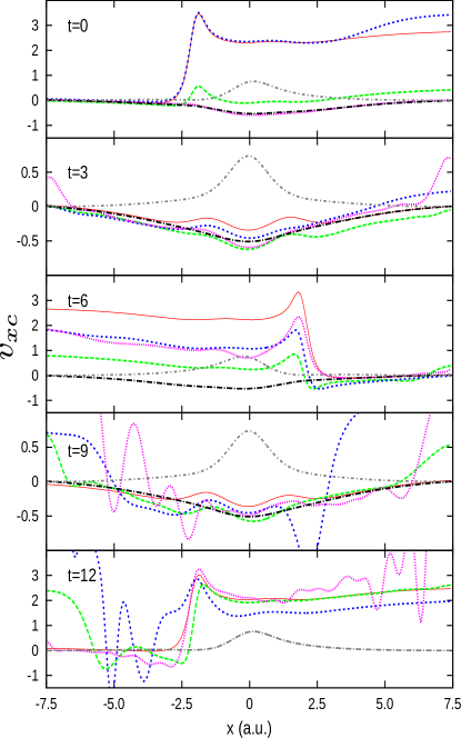
Figure 2: $v_{\scriptscriptstyle\rm XC}(x,t)$ for the different choices of KS initial state: $\Phi(0)={\Phi}^{a=0}$ (red, solid), $\Phi(0)={\Phi}^{a=1}$ (green, long-dashed), $\Phi(0)=\widetilde{\Phi}^{a=1}$ (blue, short-dashed), $\Phi(0)=\Psi(0)$ (pink, dotted) and the adiabatically-exact $v_{\scriptscriptstyle\rm XC}^{AE}$ (black, long-dashed-dot). The periodicity of the density $n(x,t)$, plotted as a guide in grey, short-dashed-dot, is $T=11.788$ a.u. The oscillations seen in the potentials at longer times are a feature of our system, and not a numerical artifact; they are converged with respect to spacing and time-step. Please note the $y$-scale changes in each plot.

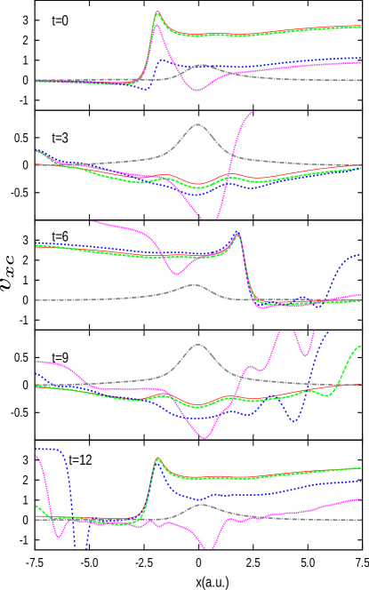
Figure 3: $v_{\scriptscriptstyle\rm XC}(x,t)$ for the different choices of KS initial state: $\Phi(0)={\Phi}^{a=0}$ (red, solid), $\Phi(0)={\Phi}^{a=0.5}$ (green, long-dashed), $\Phi(0)={\Phi}^{a=0.8}$ (blue, short-dashed), $\Phi(0)=\Phi^{a=3}$ (pink,dotted). The density $n(x,t)$ is plotted in grey, short-dashed-dot.

We observe that the exact xc potential is hugely dependent on the choice of initial state. The prominent step feature at $t=0$ seen when an SSD is used ($a=0$), which requires a non-adiabatic functional to be captured, can be significantly reduced when other choices of initial Kohn-Sham state are used. Note that although at $t=12$, in the middle region the step structure might appear more similar for several different choices of initial Kohn-Sham state than at earlier times, at later times they again become quite different, as clear in Figs 4, 5, and 6.

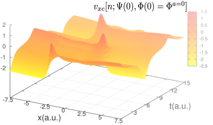
Figure 4: $v_{\scriptscriptstyle\rm XC}(x,t)$ for the SSD choice $\Phi(0)=\Phi^{a=0}$, shown up to time 15 a.u..

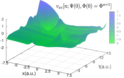
Figure 5: $v_{\scriptscriptstyle\rm XC}(x,t)$ for the choice $\Phi(0)=\Phi^{a=1}$, shown up to time 15 a.u..

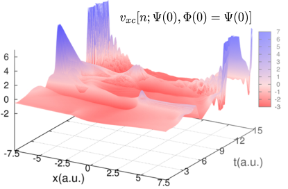
Figure 6: $v_{\scriptscriptstyle\rm XC}(x,t)$ for the choice $\Phi(0)=\Psi(0)$, shown up to time 15 a.u..

Observations for $\Phi^{a=1}$ Out of the few-determinant states (i.e. all except for the $\Phi(0)=\Psi(0)$ case), the smallest xc effects are observed at short times with state $\Phi^{a=1}$ which mimics most closely the form of the interacting initial state with non-interacting orbitals. The non-adiabatic features are smaller at short times, although still present, as can be seen by comparing with the AE plotted over the first period (since the density is periodic, and the AE depends only on the instantaneous density, the AE also just repeats over subsequent periods). For longer times though, the non-adiabatic features can get large for $\Phi^{a=1}$, where at $t=12$ au, for example, we see large oscillations in the tails and a step feature about the same size as that of the SSD case.

Observations for $\widetilde{\Phi}^{a=1}$ However, simply having the right configuration is clearly not enough: at $t=0$ the potential for the state $\widetilde{\Phi}^{a=1}$ has just as prominent a step as the SSD (${\Phi}^{a=0}$) case and a very similar shape overall, especially on the left, with small gentle differences on the right except in the right-hand tail of the density where they differ more. Looking back to Fig. 1, the potentials in which the orbitals of $\widetilde{\Phi}^{a=1}$ and ${\Phi}^{a=0}$ are eigenstates are almost identical until the initial density gets quite small on the right; in particular, they both possess a relatively sharp barrier near the minimum of the density on the left. The $\widetilde{\Phi}^{a=1}$ orbitals are trapped between this large peak and the boundary at $L/2=7.5$ (see Fig. 1). The occupied orbital of $v^{a=0}(x)$ (see upper left figure in Fig. 1) is bound but with an energy lying close to the small barrier on its right, giving it a large tunneling tail. On the other hand, $v^{a=1}(x)$ binds its lowest orbital more tightly to the position of its well, deeper than the cases of $v^{a=0}(x)$ and $\widetilde{v}^{a=1}$. Yet, these states all have the same one-particle density (Eq. 3). Returning now to the xc potential that keeps the states evolving with the same density at the initial time, Fig. 2 top panel, we observe that the step feature on the left-hand-side is also very similar for the two states $\widetilde{\Phi}^{a=1}$ and $\Phi^{a=0}$. This implies that the orbitals have a very similar local acceleration in that region Elliott et al. (2012), which is not a priori obvious. These two KS initial states have a very different nature, and their overlaps with the initial interacting state are also very different, $\langle\Psi(0)|\Phi^{a=0}(0)\rangle=0.9202$ while $\langle\Psi(0)|\widetilde{\Phi}^{a=1}(0)\rangle=0.7819$. (In fact $\langle\Psi(0)|\Phi^{a=1}(0)\rangle=0.9935$, much closer to $\langle\Psi(0)|\Phi^{a=0}(0)\rangle$, yet the resulting xc potential at the initial time is very different). At longer times, the potentials do begin to differ significantly though as expected. The large step in the potential for $\Phi^{a=0}$ dynamically oscillates in a periodic manner, while the potential for $\widetilde{\Phi}^{a=1}$ gets rather unruly quite quickly. Note that the periodicity of the density carries over to the potential for the single-orbital case ($\Phi(0)=\Phi^{a=0}$) and the AE potential, due to the fact that the single Kohn-Sham orbital depends simply and directly only on the density and its first time-derivative (see Sec III). This is not the case for the other Kohn-Sham initial states, and their periodicity is more complicated. Another striking example can be found in Nielsen et al. (2013), where the Kohn-Sham potential for a static density but with the interacting wave function as initial Kohn-Sham state is considered. The Kohn-Sham potential is strongly time-dependent since it needs to keep the static form of the density despite the rapidly changing (multi-determinantal) Kohn-Sham wave function.

Observations for the other few-determinant states The potentials for the other few-determinant states in Fig. 3 all have significant step features at the initial time and develop large oscillatory features quite quickly. The $\Phi^{a=0.5}$ case remains relatively close to the SSD case on the scale shown, while the xc potential for $\Phi^{a=3}$ has large wells and barriers throughout. The case of $\Phi^{a=0.8}$ is the one closest to the “best” few-determinant state $\Phi^{a=1}$ shown on the left for short times, but develops already a large step after half a period.

Observations for $\Phi(0)=\Psi(0)$ The choice of the (many-determinant) state $\Phi(0)=\Psi(0)$ yields a potential strikingly smaller than all the other potentials at $t=0$, which is very close to the AE potential. After already half a period however, the potential, grows for this case too, along with steps and peaks. Note that the oscillations seen after half a period are a feature of our system, and not numerical artifacts; they are converged with respect to numerical parameters.

At this point we wish to stress that it is not that we necessarily are striving to find the smallest xc potential; rather, we are trying to find one with either the smallest non-adiabatic features such that the usual adiabatic approximations would work best, or that is in some other way somehow amenable to practical approximations. Of course, the latter is not a very clearly-defined goal, however we discuss a few approaches in the next section. For now, regarding the AE approximation, we see that it is a very poor approximation for most the choices of initial state we have studied, the exception being the case $\Phi(0)=\Psi(0)$ at very short times (within a quarter of a period). We will in fact find an even better approximation to the potential for $\Phi(0)=\Psi(0)$ for very short times in the next section.

V Decompositions and Approximations of the xc potential

Often when considering approximations, it is natural to decompose the exact xc potential into parts that could be treated at different levels of approximation. We will discuss here four different types of decompositions.

Exchange and Correlation The first is the common decomposition into exchange and correlation, as has been traditionally done in ground-state density functional theory (DFT) and electronic structure theory in general. Exchange implies interaction effects beyond Hartree that account only for the Pauli exclusion principle; it arises very naturally therefore in any theory that utilizes an SSD reference, since an SSD takes care of the antisymmetry but does not introduce any other interaction effects. For example, the ground-state DFT (or Hartree-Fock) exchange energy is defined exactly as the expectation value of the electron-electron operator in the Kohn-Sham (or Hartree-Fock) SSD minus the Hartree energy. This decomposition has affected the development of functional approximations. The exchange energy is known exactly, is self-interaction-free, and dominates over correlation for atomic and molecular ground-states at equilibrium geometries. Because of this, some developers argue the exact exchange energy should be used Görling (1999), while others Baerends and Gritsenko (2005) make the case that exchange and correlation should be approximated together to make use of error cancellation, especially for the electron-pair bond in molecules where correlation becomes large. Now, in the time-dependent theory a new element arises: the possibility of using Kohn-Sham states that are not SSDs throws into question the relevance of this separation into exchange and correlation. If we were to define exchange via interaction effects beyond Hartree introduced by considering the interaction operator on a Kohn-Sham state that is not an SSD, then clearly this includes more than just the effects from the Pauli exclusion principle. If we preserve the meaning of exchange as representing Pauli exclusion then, for two electrons in a spin-singlet as we have, $v_{\scriptscriptstyle\rm X}=-v_{\scriptscriptstyle\rm H}/2$, independent of the choice of the initial Kohn-Sham state. The exchange potential therefore for any two-electron singlet dynamics is adiabatic and has the shape of a simple well “under” the density, with all the more interesting structure seen in Figs 2 and 3 appearing in the correlation potential.

Adiabatic and Non-Adiabatic The second decomposition we discuss is the usual one made in TDDFT: into adiabatic (A) and non-adiabatic (NA) (also termed dynamical) components, defined as

$$v_{\scriptscriptstyle\rm XC}[n;\Psi(0),\Phi(0)]=v_{\scriptscriptstyle\rm XC}^{\rm A}[n(t)]+v_{\scriptscriptstyle\rm XC}^{\rm NA}[n;\Psi(0),\Phi(0)]\;,$$ (12)

where

$$v_{\scriptscriptstyle\rm XC}^{\rm A}[n]=v_{\scriptscriptstyle\rm XC}^{\rm g.s.}[n]=v_{\scriptscriptstyle\rm S}^{\rm g.s.}[n]-v^{\rm g.s.}[n]-v_{\scriptscriptstyle\rm H}[n].$$ (13)

If the exact ground-state xc potential is used in Eq. (13), this defines the AE potential, which we plotted in Fig.  2 and discussed in previous section. In our specific case we have given $v_{\scriptscriptstyle\rm S}^{\rm g.s.}[n]$ explicitly in Eq. (7). For $v^{\rm g.s.}[n]$ we employed the iteration method outlined in appendix A. In practise, most calculations in TDDFT use an adiabatic approximation, setting $v_{\scriptscriptstyle\rm XC}^{\rm NA}=0$ and choosing one of the myriad approximations developed for the ground-state on the right-hand-side of Eq. (13). Given that the “best” adiabatic approximation, the AE, is not close to the exact xc potential for any of the choices of initial Kohn-Sham state except at very short times for the $\Phi(0)=\Psi(0)$ choice, it is unlikely that any adiabatic approximation will propagate accurately for this dynamics.

Kinetic and Interaction A third decomposition is in terms of kinetic and interaction components van Leeuwen (1999); Ruggenthaler and Bauer (2009); Luo et al. (2014), which has only recently been studied to understand better the nature of the xc potential, in particular the non-adiabatic step and peak features that appear in non-equilibrium dynamics Elliott et al. (2012); Luo et al. (2014). A similar decomposition was pioneered by Evert Jan Baerends and his group for the ground-state case Buijse et al. (1989); Gritsenko et al. (1994, 1996); Gritsenko and Baerends (1996), where it provided an insightful analysis of step and peak features in ground-state potentials of atoms and molecules. The ground-state xc potential is expressed in terms of kinetic, hole, and response components. The kinetic and response components display peak and step features in intershell regions in atoms, bonding regions in molecules, becoming especially prominent at large bond-lengths, where they tend to be an indication of static correlation. In the time-dependent case, we define the interaction (W) and kinetic (T) terms

$$v_{\scriptscriptstyle\rm XC}=v_{\scriptscriptstyle\rm XC}^{W}+v_{\scriptscriptstyle\rm C}^{T}$$ (14)

via Eq. (9)

$$-\partial_{x}\left(n(x,t)\partial_{x}v_{\scriptscriptstyle\rm C}^{T}(x,t)\right)= \partial_{x}\langle\Psi(t)|\hat{Q}_{\scriptscriptstyle\rm S}(x)\Psi(t)\rangle$$ (15)

$$-\partial_{x}\langle\Phi(t)|\hat{Q}_{\scriptscriptstyle\rm S}(x)\Phi(t)\rangle$$

$$-\partial_{x}\left(n(x,t)\partial_{x}v_{\scriptscriptstyle\rm XC}^{W}(x,t)\right) -\partial_{x}\left(n(x,t)\partial_{x}v_{\scriptscriptstyle\rm H}(x,t)\right)$$ (16)

$$=-i\partial_{x}\langle\Psi(t)|[\hat{j}(x),\hat{W}]\Psi(t)\rangle$$

which can be solved for as

$$v_{\scriptscriptstyle\rm XC}^{W} = \int^{x}dx^{\prime\prime}\int n_{\scriptscriptstyle\rm XC}(x^{\prime},x^{\prime\prime},t)\frac{\partial}{\partial x^{\prime\prime}}w(|x^{\prime}-x^{\prime\prime}|)dx^{\prime}$$ (17)

$$v_{\scriptscriptstyle\rm C}^{T} = \int^{x}\frac{1}{4n(x^{\prime\prime},t)}\left(\frac{d}{dx^{\prime}}-\frac{d}{dx^{\prime\prime}}\right)\left(\frac{d^{2}}{dx^{\prime\prime 2}}-\frac{d^{2}}{dx^{\prime 2}}\right)$$

$$\left(\rho_{1}(x^{\prime},x^{\prime\prime},t)-\rho_{1,S}(x^{\prime},x^{\prime\prime},t)\right)|_{x^{\prime}=x^{\prime\prime}}dx^{\prime\prime}$$

where $n_{\scriptscriptstyle\rm XC}$ is the xc hole, defined via the pair density, $P(x^{\prime},x,t)=N(N-1)\sum_{\sigma_{1}..\sigma_{N}}\int|\Psi(x^{\prime}\sigma_{1},x\sigma_{2},x_{3}\sigma_{3}..x_{N}\sigma_{N};t)|^{2}dx_{3}..dx_{N}=n(x,t)\left(n(x^{\prime},t)+n_{\scriptscriptstyle\rm XC}(x^{\prime},x,t)\right)$, and $\rho_{1}(x^{\prime},x,t)=N\sum_{\sigma_{1}..\sigma_{N}}\!\!\int dx_{2}...dx_{N}\Psi^{*}(x^{\prime}\sigma_{1},x_{2}\sigma_{2}...x_{N}\sigma_{N};t)\times\\ \Psi(x\sigma_{1},x_{2}\sigma_{2}\dots x_{N}\sigma_{N};t)$ is the spin-summed one-body density-matrix, and analogously for the Kohn-Sham system. The equations are written for the 1D case for simplicity. In Ref. Luo et al. (2014) it was shown that for the SSD choice of Kohn-Sham initial state, $\Phi^{a=0}$, both $v_{\scriptscriptstyle\rm C}^{T}$ and $v_{\scriptscriptstyle\rm XC}^{W}$ display step structure although often that in $v_{\scriptscriptstyle\rm C}^{T}$ dominates. It was found in Ref. Luo et al. (2014) that the error made by the adiabatic approximation to $v_{\scriptscriptstyle\rm C}^{T}$ is very large, typically larger than that made to $v_{\scriptscriptstyle\rm XC}^{W}$; the latter can be decomposed into the Coulomb potential of the xc hole and a correction, where the AE approximation does a fair job for the former. Although $v_{\scriptscriptstyle\rm XC}^{W}$ is independent of the choice of initial Kohn-Sham state, $v_{\scriptscriptstyle\rm C}^{T}$ is heavily dependent on it. Figure 7 plots $v_{\scriptscriptstyle\rm XC}^{W}$ and $v_{\scriptscriptstyle\rm C}^{T}$ for Kohn-Sham initial state choices $\Phi^{a=0},\Phi^{a=1},\widetilde{\Phi}^{a=1},\Psi(0)$ at several times. We see again that for the few-determinant states, $v_{\scriptscriptstyle\rm C}^{T}$ dominates the potential at the initial time and at half period ($t\sim 6$). For the choice $\Phi(0)=\Psi(0)$, $v_{\scriptscriptstyle\rm C}^{T}$ is identically zero at $t=0$; the entire xc potential is initially in the interaction term $v_{\scriptscriptstyle\rm XC}^{W}$, which is small. At later times however, $v_{\scriptscriptstyle\rm C}^{T}$ becomes large also for this choice of KS initial state.

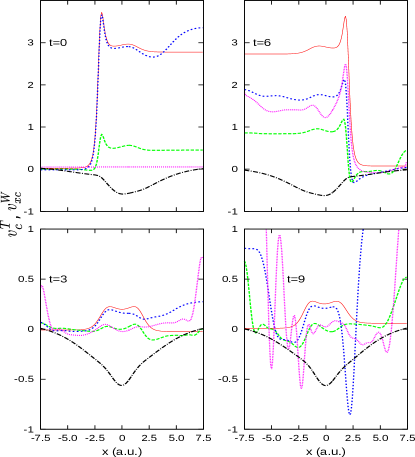
Figure 7: $v_{\scriptscriptstyle\rm C}^{T}$ for the different choices of Kohn-Sham initial state: $\Phi(0)={\Phi}^{a=0}$ (red, solid), $\Phi(0)={\Phi}^{a=1}$ (green, long-dashed), $\Phi(0)=\widetilde{\Phi}^{a=1}$ (blue, short-dashed), $\Phi(0)=\Psi(0)$ (pink, dotted). $v_{\scriptscriptstyle\rm XC}^{W}$ is independent of the choice of initial Kohn-Sham state, shown in black (dashed-dot).

Single-particle and Remainder From the previous decomposition, a natural question then arises: if we approximate $v_{\scriptscriptstyle\rm XC}^{W}$ by inserting the instantaneous Kohn-Sham xc hole on the right-hand-side of Eq (LABEL:eq:vxcW), then how well does it do? If we made the analogous approximation to $v_{\scriptscriptstyle\rm C}^{T}$, approximating the true density-matrix by the Kohn-Sham one, it would yield zero, so such an approach would have to be used either if some other approximation for $v_{\scriptscriptstyle\rm C}^{T}$ was used in conjunction, or if $v_{\scriptscriptstyle\rm C}^{T}$ itself is very small. Indeed the latter occurs when $\Phi(0)=\Psi(0)$ for very short times. At the initial time, it is clear from Eq. (V) that when $\Psi(0)=\Phi(0)$, $v_{\scriptscriptstyle\rm XC}^{T}=0$ and $v_{\scriptscriptstyle\rm XC}=v_{\scriptscriptstyle\rm XC}^{W}$. This observation motivates therefore a fourth decomposition:

$$v_{\scriptscriptstyle\rm XC}=v_{\scriptscriptstyle\rm XC}^{\scriptscriptstyle\rm S}+v_{\scriptscriptstyle\rm XC}^{\scriptscriptstyle\rm NS}$$ (19)

where the $v_{\scriptscriptstyle\rm XC}^{\scriptscriptstyle\rm S}$ represents the “single-particle” contribution

$$v_{\scriptscriptstyle\rm XC}^{\scriptscriptstyle\rm S}=\int^{x}dx^{\prime\prime}\int n_{\scriptscriptstyle\rm XC}^{\scriptscriptstyle\rm S}(x^{\prime},x^{\prime\prime},t)\frac{\partial}{\partial x^{\prime\prime}}w(|x^{\prime}-x^{\prime\prime}|)dx^{\prime}$$ (20)

where $n_{\scriptscriptstyle\rm XC}^{\scriptscriptstyle\rm S}(x^{\prime},x^{\prime\prime},t)$ is defined via $P^{\scriptscriptstyle\rm S}(x^{\prime},x,t)\equiv N(N-1)\sum_{\sigma_{1}..\sigma_{N}}\int|\Phi(x^{\prime}\sigma_{1},x\sigma_{2},x_{3}\sigma_{3}...x_{N}\sigma_{N};t)|^{2}dx_{3}..dx_{N}=n(x,t)\left(n(x^{\prime},t)+n_{\scriptscriptstyle\rm XC}^{\scriptscriptstyle\rm S}(x^{\prime},x,t)\right)$ and $v_{\scriptscriptstyle\rm XC}^{\scriptscriptstyle\rm NS}$ represents the remainder, the non-single-particle component. In fact, $v_{\scriptscriptstyle\rm XC}^{\scriptscriptstyle\rm S}$, which may be viewed as an orbital-dependent functional Ruggenthaler and Bauer (2009), is relatively simple to compute and to propagate with, so if $v_{\scriptscriptstyle\rm XC}^{\scriptscriptstyle\rm S}$ is a good approximation to $v_{\scriptscriptstyle\rm XC}$, then this would represent a promising new direction for functional development. Clearly, whether it is a good approximation or not depends strongly on the choice of the Kohn-Sham initial state. If an SSD is chosen, $v_{\scriptscriptstyle\rm XC}^{\scriptscriptstyle\rm S}$ reduces to the time-dependent exact-exchange approximation. In the general case, it includes some correlation. Our previous plots suggest that, for the field-free evolution of the 50:50 superposition state with the chosen Kohn-Sham initial states we are studying at present, although $v_{\scriptscriptstyle\rm XC}^{\scriptscriptstyle\rm S}$ may be a reasonable approximation to $v_{\scriptscriptstyle\rm XC}^{W}$ it will be a poor approximation to $v_{\scriptscriptstyle\rm XC}$ because of the dominating $v_{\scriptscriptstyle\rm XC}^{T}$ component, except for the case $\Psi(0)=\Phi(0)$ where it will be very good at short times but likely not good at longer times.

Figures 8 and 9 verify this. Figure 8 shows that $v_{\scriptscriptstyle\rm XC}^{\scriptscriptstyle\rm S}$ is an excellent approximation to $v_{\scriptscriptstyle\rm XC}^{W}$ for the case $\Phi(0)=\Psi(0)$, especially at earlier times. It is also not a bad approximation for the other initial state choices. Figure 9 compares then the approximation $v_{\scriptscriptstyle\rm XC}^{\scriptscriptstyle\rm S}$ to the full $v_{\scriptscriptstyle\rm XC}$ for the cases in which $v_{\scriptscriptstyle\rm C}^{T}$ is the smallest, $\Phi(0)=\Psi(0)$ and $\Phi(0)=\Phi^{a=1}$, along with the AE xc potential, and bears out the expectations of the previous paragraph.

The integrated nature of $v_{\scriptscriptstyle\rm XC}^{W}$ (see Eq. LABEL:eq:vxcW) makes it much more forgiving to approximate xc holes, than the $v_{\scriptscriptstyle\rm C}^{T}$ is to the density-matrix; the high number of derivatives in Eq. V make $v_{\scriptscriptstyle\rm C}^{T}$ very sensitive.

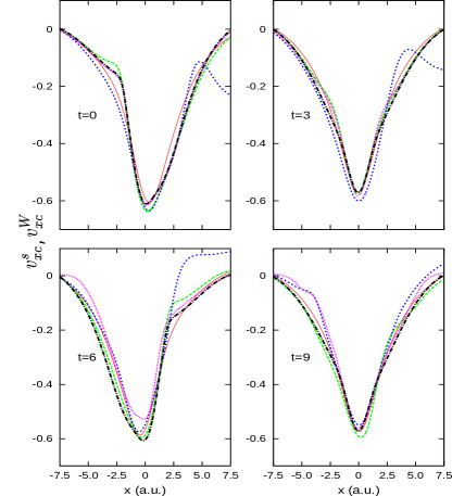
Figure 8: $v_{\scriptscriptstyle\rm XC}^{\scriptscriptstyle\rm S}$ for the different choices of Kohn-Sham initial state: $\Phi(0)={\Phi}^{a=0}$ (red, solid), $\Phi(0)={\Phi}^{a=1}$ (green, long-dashed), $\Phi(0)=\widetilde{\Phi}^{a=1}$ (blue, short-dashed), $\Phi(0)=\Psi(0)$ (pink , dotted) versus $v_{\scriptscriptstyle\rm XC}^{W}$ (black, dashed-dot). Notice that $v_{\scriptscriptstyle\rm XC}^{\scriptscriptstyle\rm S}$ approximates well $v_{\scriptscriptstyle\rm XC}^{W}$ for all choices of KS initial state, especially for the choice $\Phi(0)=\Psi(0)$ at early times.

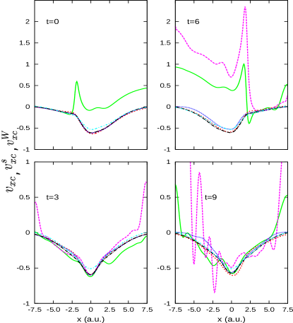
Figure 9: $v_{\scriptscriptstyle\rm XC}$ and $v_{\scriptscriptstyle\rm XC}^{\scriptscriptstyle\rm S}$ for the choices of KS initial state: $\Phi(0)={\Phi}^{a=1}$ (green solid; red short-dashed),$\Phi(0)=\Psi(0)$ (pink long-dashed; blue dotted) along with the AE xc potential (light-blue, dot-dashed) and $v_{\scriptscriptstyle\rm XC}^{W}$ (black, dot-long-dashed).

VI Conclusions and Outlook

Initial-state dependence is a subtle aspect of the exact xc potential of TDDFT that has no precedent in ground-state DFT. Here we have explored the possibility of exploiting it to ease the job of the xc functional, i.e. to investigate whether, for a given initial state of the interacting problem, there is a “most suitable” Kohn-Sham initial state to use such that features of the xc functional are simpler to approximate. We note that most calculations today assume an SSD for the Kohn-Sham system, but the theory has no such restriction. We have focussed only on one case, field-free evolution of a 50:50 superposition of a ground and first-excited state of a two-electron problem. This is, arguably, one of the most difficult cases for conventional approximations in TDDFT, given the extreme non-equilibrium nature of the dynamics. At the same time, although the results here are discussed specifically for this particular evolution, they have consequences also for dynamics driven by external fields when beginning in the ground state, since such superpositions can be reached in the interacting system, yet the Kohn-Sham state at all times is restricted to whatever configuration it began in.

Earlier work had shown that if an SSD is chosen as the Kohn-Sham state, large dynamical features, such as steps and peaks, appear in the potential from the very onset of the dynamics. These are completely missed by any adiabatic approximation and have a dependence on the density that is non-local in space and time. It has remained so far a challenge to derive approximate density-functionals with memory that incorporate these features, and so adds much motivation to the complementary path we investigate here, whether one can exploit initial-state dependence to reduce their size.

We have found that if the Kohn-Sham state is chosen to also have the form of a 50:50 superposition state, then one can find such a state for which the non-adiabatic step and peak features are small at short times. But at longer times (in our case, within one period of the dynamics), the non-adiabatic features can get large, as large as the SSD choice. However simply having the right configuration is not enough; other initial states with this configuration can be found for which the non-adiabatic features are again large even at short times. Having said that, perhaps there is another Kohn-Sham state of this form that we just did not find, that has actually smaller non-adiabatic features. If we instead consider the correlated many-body interacting state as the initial Kohn-Sham state, then we find that at very short times, the adiabatic approximation becomes a very accurate approximation to the xc potential, however even after half a period, dynamical step and peak features reappear that are larger than the best few-determinant choice. We can conclude that for very short times, the choice of $\Phi(0)=\Psi(0)$ is best if one must use an adiabatic approximation, while at longer but still short times (on the time-scale of the dynamics), a judicious choice of a Kohn-Sham initial state with the same configuration as the interacting state is likely a better choice. This particular conclusion is not universally true, e.g. if the initial interacting state is a ground state, then the adiabatic approximation works best at short times if the Kohn-Sham state is a non-interacting ground-state, and the AE becomes then exact at the initial time Elliott and Maitra (2012).

We propose a new direction for developing approximations for the xc potential in cases where the Kohn-Sham state is chosen generally (i.e. not restricted to an SSD). This is based on decomposing the exact expression for the xc potential arising from the force-balance equation of TDDFT into a single-particle component and the remainder. One can express the exact xc potential as two contributions, one is a kinetic term, and the other is an interaction term. The single-particle component, $v_{\scriptscriptstyle\rm XC}^{\scriptscriptstyle\rm S}$ has only terms arising from the interaction, but evaluated using the Kohn-Sham xc hole; it reduces therefore to exchange in the SSD limit, but in the general case, includes correlation components too. It is straightforward to compute as an orbital functional, and we found that, for initial Kohn-Sham states judiciously chosen as discussed above, it gives an extremely good approximation to the exact interaction term, and a very good approximation to the full xc potential for short times. At longer times, the kinetic term becomes important and $v_{\scriptscriptstyle\rm XC}^{\scriptscriptstyle\rm S}$ becomes inaccurate. Future work involves focussing then on developing new approximations for the kinetic component of the xc potential while utilizing $v_{\scriptscriptstyle\rm XC}^{\scriptscriptstyle\rm S}$ for the interaction component.

Appendix A Finding adiabatic potentials and eigenstates for a given density and current

To find a potential $v(x)$ for a given form of the Hamiltonian, i.e., interacting or non-interacting, that has an eigenstate which reproduces a given density $n(x)$ and current density $j(x)=0$, we employ an iterative method along the lines of van Leeuwen van Leeuwen and Baerends (1994). The iteration steps read

$$v_{k+1}(x)=v_{k}(x)+\delta\left(\frac{n_{k}(x)}{n(x)}-1\right),$$ (21)

where $n_{k}(x)$ is the density of the eigenstate of $v_{k}(x)$ and we choose $\delta>0$ small enough. We see that the procedure in each iteration simply increases the potential where the density is too large, to push away density, and decreases the potential where the density is too small, to collect more density. If we prescribe a ground-state density (no nodes) and use the ground-state density $n_{k}(x)$ of $v_{k}(x)$ in each iteration then, if the procedure converges, the solution is a unique ground-state due to the Hohenberg-Kohn uniqueness theorem. In this way we can determine the ground-state potentials $v^{\rm g.s.}[n](x)$ (see Eq. (13) and discussion thereafter) in the interacting case. This would also work in the non-interacting case, but in our two-particle spin-singlet case the ground-state potential in the non-interacting case is known explicitly and hence we can directly use Eq. (7).
On the other hand, if we restrict the form of our Kohn-Sham wave function $\Phi^{(a\neq 0)}$ in the above iteration scheme and thus have

$$n^{(a)}(x)=\frac{(2+a^{2})\phi_{0}(x)^{2}+2\sqrt{2}a\phi_{0}(x)\phi_{1}(x)+a^{2}\phi_{1}(x)^{2}}{(1+a^{2})},$$ (22)

we are constructing an excited state of a non-interacting problem. Hence, if we converge, we can no longer rely on the Hohenberg-Kohn uniqueness theorem and consequently we can find several solutions, such as in the case $a=1$ (see cases (ii) and (iii) in section II).

References

- Ullrich (2011) C. A. Ullrich, Time-dependent density-functional theory: concepts and applications (Oxford University Press, 2011).
- Marques et al. (2012) M. A. Marques, N. T. Maitra, F. M. Nogueira, E. K. Gross, and A. Rubio, eds., Fundamentals of time-dependent density functional theory, Vol. 837 (Springer, 2012).
- Runge and Gross (1984) E. Runge and E. K. U. Gross, Phys. Rev. Lett. 52, 997 (1984).
- van Leeuwen (1999) R. van Leeuwen, Phys. Rev. Lett. 82, 3863 (1999).
- Rozzi et al. (2013) C. A. Rozzi, S. M. Falke, N. Spallanzani, A. Rubio, E. Molinari, D. Brida, M. Maiuri, G. Cerullo, H. Schramm, J. Christoffers, et al., Nature Communications 4, 1602 (2013).
- Penka Fowe and Bandrauk (2011) E. Penka Fowe and A. D. Bandrauk, Phys. Rev. A 84, 035402 (2011).
- Shinohara et al. (2012) Y. Shinohara, S. Sato, K. Yabana, J.-I. Iwata, T.Otobe, and G. F. Bertsch, J. Chem. Phys 137, 22A527 (2012).
- Elliott et al. (2016) P. Elliott, K. Krieger, J. K. Dewhurst, S. Sharma, and E. K. U. Gross, New Journal of Physics 18, 013014 (2016).
- Raghunathan and Nest (2011) S. Raghunathan and M. Nest, J. Chem. Theory and Comput. 7, 2492 (2011).
- Raghunathan and Nest (2012) S. Raghunathan and M. Nest, J. Chem. Theory and Comput. 8, 806 (2012).
- Habenicht et al. (2014) B. F. Habenicht, N. P. Tani, M. R. Provorse, and C. M. Isborn, J. Chem. Phys. 141, 184112 (2014).
- Ramsden and Godby (2012) J. Ramsden and R. Godby, Phys. Rev. Lett. 109, 036402 (2012).
- Hodgson et al. (2013) M. J. P. Hodgson, J. D. Ramsden, J. B. J. Chapman, P. Lillystone, and R. W. Godby, Phys. Rev. B 88, 241102 (2013).
- Hodgson et al. (2014) M. J. P. Hodgson, J. D. Ramsden, T. R. Durrant, and R. W. Godby, Phys. Rev. B 90, 241107 (2014).
- Elliott et al. (2012) P. Elliott, J. I. Fuks, A. Rubio, and N. T. Maitra, Phys. Rev. Lett. 109, 266404 (2012).
- Fuks et al. (2013) J. I. Fuks, P. Elliott, A. Rubio, and N. T. Maitra, J. Phys. Chem. Lett. 4, 735 (2013).
- Luo et al. (2014) K. Luo, J. I. Fuks, E. D. Sandoval, P. Elliott, and N. T. Maitra, J. Chem. Phys 140, 18A515 (2014).
- Luo et al. (2013) K. Luo, P. Elliott, and N. T. Maitra, Phys. Rev. A 88, 042508 (2013).
- Buijse et al. (1989) M. A. Buijse, E. J. Baerends, and J. G. Snijders, Phys. Rev. A 40, 4190 (1989).
- Gritsenko et al. (1994) O. V. Gritsenko, R. van Leeuwen, and E. J. Baerends, The Journal of Chemical Physics 101, 8955 (1994).
- Gritsenko et al. (1996) O. V. Gritsenko, R. van Leeuwen, and E. J. Baerends, The Journal of Chemical Physics 104, 8535 (1996).
- Gritsenko and Baerends (1996) O. V. Gritsenko and E. J. Baerends, Phys. Rev. A 54, 1957 (1996).
- Elliott and Maitra (2012) P. Elliott and N. T. Maitra, Phys. Rev. A 85, 052510 (2012).
- Nielsen et al. (2013) S. Nielsen, M. Ruggenthaler, and R. van Leeuwen, Europhys. Lett. 101, 33001 (2013).
- Nielsen et al. (2014) S. Nielsen, M. Ruggenthaler, and R. van Leeuwen, arXiv preprint arXiv:1412.3794 (2014).
- Ruggenthaler and van Leeuwen (2011) M. Ruggenthaler and R. van Leeuwen, EPL (Europhysics Letters) 95, 13001 (2011).
- Ruggenthaler et al. (2012) M. Ruggenthaler, K. Giesbertz, M. Penz, and R. van Leeuwen, Physical Review A 85, 052504 (2012).
- Penz and Ruggenthaler (2011) M. Penz and M. Ruggenthaler, Journal of Physics A: Mathematical and Theoretical 44, 335208 (2011).
- Ruggenthaler et al. (2015) M. Ruggenthaler, M. Penz, and R. van Leeuwen, Journal of Physics: Condensed Matter 27, 203202 (2015).
- Thiele et al. (2008) M. Thiele, E. K. U. Gross, and S. Kümmel, Phys. Rev. Lett. 100, 153004 (2008).
- Ruggenthaler and Bauer (2009) M. Ruggenthaler and D. Bauer, Physical Review A 80, 052502 (2009).
- Javanainen et al. (1988) J. Javanainen, J. H. Eberly, and Q. Su, Phys. Rev. A 38, 3430 (1988).
- van Leeuwen and Baerends (1994) R. van Leeuwen and E. J. Baerends, Phys. Rev. A 49, 2421 (1994).
- Ruggenthaler et al. (2013) M. Ruggenthaler, S. E. B. Nielsen, and R. Van Leeuwen, Physical Review A 88, 022512 (2013).
- Schmitteckert et al. (2013) P. Schmitteckert, M. Dzierzawa, and P. Schwab, Phys. Chem. Chem. Phys. 15, 5477 (2013).
- Fuks and Maitra (2014) J. I. Fuks and N. T. Maitra, Phys. Chem. Chem. Phys. 16, 14504 (2014).
- Karlsson et al. (2011) D. Karlsson, A. Privitera, and C. Verdozzi, Phys. Rev. Lett. 106, 116401 (2011).
- Verdozzi et al. (2011) C. Verdozzi, D. Karlsson, M. P. von Friesen, C.-O. Almbladh, and U. von Barth, Chemical Physics 391, 37 (2011), open problems and new solutions in time dependent density functional theory.
- Tokatly (2005) I. V. Tokatly, Phys. Rev. B 71, 165104 (2005).
- Görling (1999) A. Görling, Phys. Rev. Lett. 83, 5459 (1999).
- Baerends and Gritsenko (2005) E. J. Baerends and O. V. Gritsenko, The Journal of Chemical Physics 123, 062202 (2005), http://dx.doi.org/10.1063/1.1904566.