Constraining the physical structure of the inner few 100 AU scales of deeply embedded low-mass protostars.

Abstract

Context. The physical structure of deeply embedded low-mass protostars (Class 0) on scales of less than 300 AU is still poorly constrained. While molecular line observations demonstrate the presence of disks with Keplerian rotation toward a handful of sources, others show no hint of rotation. Determining the structure on small scales (a few 100 AU) is crucial for understanding the physical and chemical evolution from cores to disks.

Aims. We determine the presence and characteristics of compact, disk-like structures in deeply embedded low-mass protostars. A related goal is investigating how the derived structure affects the determination of gas-phase molecular abundances on hot-core scales.

Methods. Two models of the emission, a Gaussian disk intensity distribution and a parametrized power-law disk model, are fitted to subarcsecond resolution interferometric continuum observations of five Class 0 sources, including one source with a confirmed Keplerian disk. Prior to fitting the models to the de-projected real visibilities, the estimated envelope from an independent model and any companion sources are subtracted. For reference, a spherically symmetric single power-law envelope is fitted to the larger scale emission ($\sim$1000 AU) and investigated further for one of the sources on smaller scales.

Results. The radii of the fitted disk-like structures range from $\sim 90-170$ AU, and the derived masses depend on the method. Using the Gaussian disk model results in masses of $54-556\times 10^{-3}$ $M_{\rm\sun}$, and using the power-law disk model gives $9-140\times 10^{-3}$ $M_{\rm\sun}$. While the disk radii agree with previous estimates the masses are different for some of the sources studied. Assuming a typical temperature distribution ($r^{-0.5}$), the fractional amount of mass in the disk above 100 K varies from 7% to 30%.

Conclusions. A thin disk model can approximate the emission and physical structure in the inner few 100 AU scales of the studied deeply embedded low-mass protostars and paves the way for analysis of a larger sample with ALMA. Kinematic data are needed to determine the presence of any Keplerian disk. Using previous observations of p-H${}_{2}^{18}$O, we estimate the relative gas phase water abundances relative to total warm H₂ to be $6.2\times 10^{-5}$ (IRAS 2A), $0.33\times 10^{-5}$ (IRAS 4A-NW), $1.8\times 10^{-7}$ (IRAS 4B), and $<2\times 10^{-7}$ (IRAS 4A-SE), roughly an order of magnitude higher than previously inferred when both warm and cold H₂ were used as reference. A spherically symmetric single power-law envelope model fails to simultaneously reproduce both the small- and large-scale emission.

1 Introduction

A gravitationally collapsing core of gas and dust marks the beginning of the star formation process in molecular clouds. These infall-dominated pre-stellar cores evolve into envelope dominated, Class 0 sources with well-collimated bipolar outflows (André et al. 2000), hinting at the presence of a disk. Once the accretion has progressed enough, the source is classified as a disk dominated Class I source, characterized by a more tenuous envelope and a rotating circumstellar disk (e.g., Jørgensen et al. 2009; Beckwith et al. 1989; Beckwith & Sargent 1993; ALMA Partnership et al. 2015). In the subsequent Class II stage (T Tauri source), the envelope has almost completely dissipated and the disk is characterized by Keplerian rotation and may have developed cavities (Guilloteau & Dutrey 1994; Qi et al. 2003; Simon et al. 2000; Williams & Cieza 2011; Espaillat et al. 2014). Although there is evidence for disks at all stages of protostellar evolution, they have not yet been characterized in the earliest stages. Early simulations of collapsing rotating clouds show that large-scale ($\sim 1000$ AU) flattened infalling envelopes with small-scale ($\sim 100$ AU) disks are expected to form (e.g., Cassen & Moosman 1981; Terebey et al. 1984; Galli & Shu 1993). Tracing the evolution of disks through the entire star formation process will make it possible to determine when and how disks form and evolve. The physical characteristics of this early structure therefore mark the starting point of disk evolution studies.

Interferometric observations of deeply embedded low-mass protostars taken with a resolution of few arcseconds have revealed unresolved compact components on scales $<300$ AU (e.g., Hogerheijde et al. 1999; Looney et al. 2003; Harvey et al. 2003; Jørgensen et al. 2005b), and these structures are not fit well by standard envelope models. Rotating disks with sizes of $R<50\sim 200$ AU have been found for a few Class 0 sources based on kinematical analysis on the molecular lines (e.g., Tobin et al. 2012; Murillo et al. 2013b; Ohashi et al. 2014; Lindberg et al. 2014; Lee et al. 2014). This raises the questions of how early such disks form after collapse and how common they are. High-resolution C¹⁸O observations toward other Class 0 sources show velocity gradients perpendicular to the outflow toward some sources (Yen et al. 2015), but not necessarily in a rotationally supported disk (Brinch et al. 2009; Maret et al. 2014). Thus, the physical conditions (i.e., density, temperature, mass) of deeply embedded low-mass protostars on small scales are poorly constrained.

The density and temperature structure on small scales also affect the chemistry and derived abundances. Some low-mass protostars show strong lines of complex organic molecules that are thought to originate from regions where the dust temperature exceeds 100 K and all ices have been sublimated (e.g., van Dishoeck & Blake 1998; Bottinelli et al. 2004; Herbst & van Dishoeck 2009; Öberg et al. 2014). These “hot core” or “hot corino” regions are small (radii less than 100 AU), and abundances with respect to H₂ are often inferred through comparison with a spherically symmetric power-law envelope structure, with all material inside the 100 K radius assumed to contain sublimated ice material. However, in a disk-like structure some fraction of this dust on a small scale may be much cooler than 100 K (e.g., Harsono et al. 2014, 2015). This means that the abundances of species that are only thought to exist in regions $>$100 K may have been underestimated. A prominent example is water itself: lines of H${}_{2}^{18}$O have been imaged in low-mass protostars on subarcsecond scales but inferred hot core abundances are more than an order of magnitude lower than expected from water ice sublimation (e.g., Jørgensen & van Dishoeck 2010a; Persson et al. 2012, 2013; Visser et al. 2013). Water, in turn, controls available reaction routes for other species (e.g., H₂O destroying HCO⁺; Jørgensen et al. 2013).

The temperature and density structures of the envelope on larger scales (several 1000 AU) is relatively well characterized through modeling of the spectral energy distribution and the single-dish submillimeter continuum spatial structure (e.g., Jørgensen et al. 2002; Kristensen et al. 2012) and through extinction mapping at infrared wavelengths (e.g., Tobin et al. 2010). To what extent continuum observations can be used to probe the small-scale structures, and the related transition from the large-scale envelope, is not yet clear.

With the increased sensitivity of interferometric data, it is now possible to routinely obtain subarcsecond resolution continuum interferometric observations at mm wavelengths. Here we analyze such data for five deeply embedded low-mass protostars (Class 0), including one source for which the presence of a Keplerian rotating disk has been established from kinematic data. After removing any large-scale envelope contribution, two different models are fitted to the de-projected binned real visibility amplitudes, a Gaussian intensity distribution, and a parametrized disk model. Although this analysis cannot determine whether rotationally supported disks are present, it can constrain the basic parameters of any flattened, compact disk-like structure such as radius and mass. The method presented here is intended as a proof of concept that such structures can indeed be characterized and that they have consequences for inferred abundances of species such as water. These methods can subsequently be extended and applied to current/future ALMA observations of a large sample of low-mass protostars and to additional molecules.

2 Sample and observations

Five sources were considered in this study, the four protostars IRAS 2A, IRAS 4A-NW, IRAS 4A-SE, and IRAS 4B in the NGC 1333 star forming region (235 pc, Hirota et al. 2008) and VLA 1623 in the $\rho$ Ophiuchus star forming region (120 pc, Loinard et al. 2008). The last source has a confirmed Keplerian disk with a radius of $\sim$150 AU as inferred from high-resolution C¹⁸O data (Murillo et al. 2013b).

Observational data come from several programs. The continuum toward NGC 1333 IRAS 2A and 4B at 203.4 GHz has been obtained with the Plateau de Bure Interferometer (PdBI) by Jørgensen & van Dishoeck (2010a) and Persson et al. (2012). One track ($\sim$8 hours) of complimentary A configuration (extended) data were obtained for IRAS 4B on 2 February 2011. Phase and amplitude were calibrated on the quasar 0333+321, and the absolute flux on the blazar 3C454.3. The calibration and imaging was done in IRAM GILDAS. The observations of IRAS 4B cover (projected) baselines from 12–515 $k\lambda$ (21″–0$\aas@@fstack{\prime\prime}$5), and for IRAS 2A they cover 10.5–307 $k\lambda$ (23″-0$\aas@@fstack{\prime\prime}$8). IRAS 4A was observed with the Submillimeter Array (SMA) at 335 GHz (Lai et al. in prep). The observations of IRAS 4A cover baselines from 10–510 $k\lambda$ (25″–0$\aas@@fstack{\prime\prime}$5). Finally, the ALMA Cycle 2 VLA 1623 data are from Murillo et al. (2015) at 219.0 GHz and cover baselines from 13.8–796.6 $k\lambda$ (18″–0$\aas@@fstack{\prime\prime}$3). The various source parameters are summarized in Table 1 and the sensitivity, beam, and peak fluxes for the observations are listed in Table 2.

Table 1: Parameters for the studied sources.

Source	$L_{\mathrm{bol}}$	$M_{\mathrm{env}}$	$T_{\mathrm{bol}}$	$d$
	($L_{\odot}$)	($M_{\odot}$)	($K$)	(pc)
IRAS 2A	$35.7$	$5.1$	$50$	235
IRAS 4A	$9.1$	$5.6$	$33$	235
IRAS 4B	$4.4$	$3.0$	$28$	235
VLA 1623 A	$1.1$	$0.22$	$10$	120

The resulting continuum maps from standard imaging (natural weighting, Hogbom CLEAN algorithm) are shown in Fig. 1. IRAS 4A is a resolved binary system (Looney et al. 2000; Reipurth et al. 2002; Girart et al. 2006), separated by 1$\aas@@fstack{\prime\prime}$8 where both components are relatively strong (NW and SE). VLA 1623 is a triple system in the $\rho$ Ophiuchus star forming region where one of the sources (source A) is the Class 0 object with a known Keplerian disk (Murillo & Lai 2013a; Murillo et al. 2013b); the closest companion is $\sim 1$″ away (source B) and the second, which is significantly weaker at mm wavelengths, is $\sim 10$″ to the east (source W).

Toward IRAS 2A, Codella et al. (2014) reported two secondary continuum sources that are 2″ and 2.4″ away, one along the blueshifted outflow and one southwest of the main component. Tobin et al. (2015a) show that IRAS 2A is a binary on 0$\aas@@fstack{\prime\prime}$6 scales from high sensitivity VLA observations at mm and cm wavelengths, confirming earlier speculations based on the quadruple outflow (Jørgensen et al. 2004). The two secondary continuum sources (with $>$5$\sigma$ peak) found by Codella et al. at 2^′′ offset (sensitivity of 1.5 mJy/beam) are also not seen in our high-sensitivity PdBI data (1.6 mJy/beam). Our spatial resolution and sensitivity are not high enough to confirm the close companion found by Tobin et al. This unresolved companion is significantly weaker than the main source ($<3$% at 1.3 mm, i.e., 1.65$\sigma$); therefore, it will modify the amplitude in a well-behaved manner (a very low constant value).

The continuum observations of IRAS 4B are dynamic range limited, the peak flux is $128\sigma_{\mathrm{RMS}}$, and the limit for PdBI is at $\sim 80\sigma_{\mathrm{RMS}}$ (depending on $\mathit{u}$-$\mathit{v}$ coverage, for example). This causes the low-flux compact deconvolution artifacts surrounding the continuum peak. This is not a problem since the analysis is conducted in the $\mathit{u}$-$\mathit{v}$-plane.

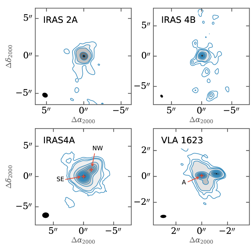
Figure 1: Maps of the continuum toward IRAS 2A (PdBI), IRAS 4B (PdBI), IRAS 4A (SMA), and VLA 1623 (ALMA). Contours start at 3$\sigma_{\mathrm{RMS}}$ in steps of 3$\sigma_{\mathrm{RMS}}$ until 9$\sigma_{\mathrm{RMS}}$, then in steps of 20$\sigma_{\mathrm{RMS}}$ ($\sigma_{\mathrm{RMS}}$ in Table 2). We note the absence of any 2″ triple toward IRAS 2A. The observations of IRAS 4B are dynamic range limited, causing convolution artifacts to appear around the compact continuum peak; these artifacts are not real (see text).

Table 2: Parameters for the continuum observations.

Source	$\sigma_{\mathrm{RMS}}$	Peak	Beam
	(mJy/beam)	($\times\sigma_{\mathrm{RMS}}$)	($\arcsec$)
IRAS 2A	1.6	55	$0.7\times 0.9$ (63∘)
IRAS 4A	10	221	$1.1\times 1.3$ (90∘)
IRAS 4B	2	128	$0.5\times 0.6$ (37∘)
VLA 1623 A	0.6	140	$0.3\times 0.5$ (92∘)

3 Models

Images from radio interferometers combine the information obtained from all baselines (scales) into one image. Thus, analyzing an image of a small-scale structure whose emission constitutes only a fraction of the total is not optimal. Visibilities provide a better starting point for taking advantage of the full information of emission on different size scales. This way the large-scale envelope can be disentangled from emission on small scales. A large-scale, roughly spherical envelope model and possible companion source(s) are subtracted (and the data de-projected), then two different models are fitted to the residuals to study the small-scale structure in these five sources. The two fitted models are an intensity distribution consisting of a Gaussian plus a point source, and an analytical equation of the visibilities given by a passively heated thin disk. Simple power-law models to the visibilities without subtracting any large-scale envelope components are provided for comparison in Sect. 5.3 for NGC 1333 IRAS 2A and in the Appendix for the rest of the sources.

3.1 Envelope model

Class 0 sources are deeply embedded in their surrounding envelope whose emission makes a non-negligible contribution to the total flux. The envelope contribution to the flux falls off with decreasing scale probed.

To analyze the smallest scales where the emission deviates from a smooth symmetric structure, we first need to remove the larger scale envelope contribution. This is done by simulating observations of model images of already published models for the envelopes of the studied sources and then subtracting them from the observations (see Fig. 2 for an example and Appendix A for all sources). The envelope models are taken to be spherically symmetric and constrained by a simultaneous fit to the SED and millimeter continuum radial profiles obtained with single-dish observations, probing scales of thousands of AU (Jørgensen et al. 2002; Kristensen et al. 2012). The most recent models include far-infrared measurements from Herschel to constrain the peak of the SED (Karska et al. 2013). The density profile is a power law given as

$$\rho_{\mathrm{env}}(r)=\rho_{\mathrm{in}}\left(\dfrac{r}{r_{\mathrm{in}}}\right)^{-p_{\mathrm{env}}},$$ (1)

where $\rho_{\mathrm{in}}=n_{\mathrm{in}}\,\mu_{\mathrm{H_{2}}}m_{p}$ and $\mu_{\mathrm{H_{2}}}\ =2.8$ (H₂, H, He, and 2% metals; Kauffmann et al. 2008, Appendix A.1), $m_{p}$ the mass of a proton and $n_{\mathrm{in}}$ the number density at $r_{\mathrm{in}}$, the inner radius of the envelope.

Instead of interpolating the density and temperature to a finer grid from the published envelope models, a model image of the envelope was created from scratch for use in simulating the visibilities appropriate for the resolution of the interferometric observations. For a best-fit density distribution, we calculate the dust temperature self-consistently at each radius of the envelope for the observed luminosity using the dust continuum radiative transfer code TRANSPHERE (Dullemond et al. 2002). The dust density and temperature structure is then input to the Monte Carlo radiative transfer code RATRAN (Hogerheijde & van der Tak 2000) to produce the model image of the continuum (assuming a gas-to-dust ratio of $\Delta_{g/d}=100$). The opacities are taken from Ossenkopf & Henning (1994). This opacity at 203.4 and 219 GHz is 0.899 cm²g^-1 and 2.57 at 335 GHz.

Because the envelope model is subtracted from the observational data, the center position of the large-scale envelope needs to be determined. This is assumed to be the continuum peak position in the interferometric data or, if there are nearby companions, the center of the large-scale emission of the system. This large-scale emission is determined from the short $\mathit{u}$-$\mathit{v}$ distances and is characterized by a Gaussian, the center of which is assumed to give the center of mass of the large-scale envelope.

The resulting model image from the radiative transfer code is then input, together with the shifted observed visibility data, to the GILDAS routine uv_fmodel. The routine simulates observations of the model image by sampling the same $\mathit{u}$-$\mathit{v}$ coverage as the observations. This envelope model is then subtracted from the observed visibilities. What is left is the contribution to the flux that cannot be attributed to such a spherical envelope alone, assuming that the envelope is optically thin.

3.2 Gaussian intensity distribution

As a first characterization of the visibilities after envelope subtraction, a Gaussian intensity distribution with an unresolved point source is fitted. The model corresponds to the emission from an embedded disk where the added unresolved point source is needed to reproduce the emission on the longest baselines. Most of the emission ($95\%$) of a Gaussian is emitted within $\pm 1\sigma\sim 0.85\times\theta_{\mathrm{FWHM}}$. From the fit we can then get an estimate of the radius of the disk/compact structure, which is taken as $r_{c}=R=0.42\times\theta_{\mathrm{FWHM}}$. Expressing the FWHM ($\theta_{FWHM}$) in arcseconds and the $\mathit{u}$-$\mathit{v}$ distance ($r_{uv}=\sqrt{u^{2}+v^{2}}$) in wavelengths, the function to fit a Gaussian intensity distribution with amplitude $F_{G}$ takes the form

$$F_{\mathrm{re}}(r_{uv})=F_{ps}+F_{G}\exp\left[-\dfrac{\left(\dfrac{\pi}{180}\dfrac{\pi\theta_{\mathrm{FWHM}}r_{uv}}{60^{2}}\right)^{2}}{4\ln 2}\right].$$ (2)

The point source flux ($F_{ps}$) is simply a constant across all $\mathit{u}$-$\mathit{v}$ distances (i.e., Fourier transform of a Dirac delta function at the origin). This assumes that the structure is circularly symmetric and the center of mass is at the phase center, so the expected imaginary amplitude is zero for all baselines.

The gas mass of the structure at a distance $d$ is calculated as

$$M=\dfrac{F_{\nu}\ d^{2}}{\kappa_{\nu}B_{\nu}\left(T\right)}\Delta_{\mathrm{g/d}},$$ (3)

where $F_{\nu}$ is the flux, $B_{\nu}(T)$ the Planck function at frequency $\nu$ and temperature $T$, $\kappa_{\nu}$ the opacity at frequency $\nu$, and $\Delta_{\mathrm{g/d}}$ the gas-to-dust-ratio. The mass is calculated using the flux of the Gaussian and point source, i.e., $F_{ps}+F_{G}$, and assumes an average temperature of 30 K. This temperature could be lower, which would increase the mass (e.g., Jørgensen et al. 2009; Dunham et al. 2014)

3.3 Power-law disk

The Gaussian model described above approximates the intensity distribution from a disk. Except for an estimate of the radius and the mass of such a disk, it does not fit any physical structure. It is possible to calculate the visibilities corresponding to an inclined circular disk with a power-law density and temperature profile (Berger & Segransan 2007). Thus, the fit will be sensitive to the physical conditions provided that such a disk is a good enough approximation of the physical structure. We note, however, that fitting observations at only one frequency is essentially a fit of $p+q$, i.e., the temperature and density together. To break the degeneracy, a temperature or density profile needs to be assumed or constrained by other means.

The model of the disk is at the phase center making the imaginary visibilities zero. A vertical disk structure is not included in the model. The radius of the disk, $r_{c}$, comes from the Gaussian fit previously described and the inner radius is set to 0.1 AU.

The temperature in the disk is given by

$$T(r)=T_{0}\left(\dfrac{r}{r_{T_{0}}}\right)^{-q},$$ (4)

where $T_{0}$ is taken to be $1500$ K at $r_{T_{0}}=0.1$ AU. We assume $q=0.5$ for all modeled disks. This is a reasonable value given both analytical studies and observations. A model of a radiative, passive circumstellar disk in hydrostatic equilibrium gives $q=0.5$ (Chiang et al. 2001, extended model of Chiang & Goldreich 1997). Observations of more evolved disks (i.e., T Tauri disks) show $0.4<q<0.75$ (Andrews & Williams 2005) confirming that $q=0.5$ is a reasonable value. This means that the 100 K radius is $r_{100\leavevmode\nobreak\ \mathrm{K}}=r_{T_{0}}(100/T_{0})^{1/-q}$, i.e., 22.5 AU for the sources in this study. Such a large value of the water snowline is consistent with 2D radiative transfer models that explicitly include the accretional heating due to high mass accretion rates expected in Class 0 systems (Harsono et al. 2015). The lowest temperature allowed in the disk is $T_{\mathrm{min}}=10$ K. This is set by the external radiation field which heats the outer envelope to similar temperatures. The surrounding envelope at $r=300$ AU is roughly $T=20-50$ K, given by the envelope models of the sources (see Sect. 3.1 and Sect. 4.2). A lower disk temperature compared to the envelope at similar radii could be explained by the expected shielding of the disk mid-plane. However, $q$ has not been accurately determined in these systems, and is not necessarily constant with radius (e.g., Whitney et al. 2003a).

The surface (dust) density as a function of radius in the disk is given by

$$\Sigma_{\mathrm{disk}}(r)=\dfrac{\Sigma_{0}}{\Delta_{\mathrm{g/d}}}\left(\dfrac{r}{r_{0}}\right)^{-p}\qquad r<r_{c},$$ (5)

$$\Sigma_{\mathrm{taper}}(r)=\dfrac{\Sigma_{c}}{\Delta_{\mathrm{g/d}}}\exp{\left[-\left(\dfrac{r}{r_{c}}\right)^{2-p}\right]}\qquad r\geq r_{c},$$ (6)

where $r_{0}$ is the reference radius and $\Sigma_{0}$ (gas density) is expressed, and $\Sigma_{c}=\Sigma_{\mathrm{disk}}(r_{c})\Delta_{g/d}$ beyond the disk critical radius $r_{c}$. The optical depth $\tau$ is given by the surface dust density multiplied with the opacity $\kappa_{\nu}$ and divided by the inclination $\cos i$, i.e., $\tau(r)=\Sigma(r)\kappa_{\nu}/\cos i$. The visibility for a given $\mathit{u}$-$\mathit{v}$ distance of such a disk can be calculated by integrating thin circular rings, each with a temperature and optical depth assuming blackbody emission (Berger & Segransan 2007),

$$V(r_{uv})=\int\dfrac{2\pi{r}}{D^{2}}B_{\nu}(T(r))\ \cos i\ \left(1-e^{-\tau(r)}\right)\ J_{0}(\dfrac{2\pi r_{uv}r}{D})\ dr,$$ (7)

where $r_{uv}$ is the projected baseline expressed in wavelengths (cf. $\theta=1.22\lambda/D$, where D is the baseline length), and all terms are expressed in cgs units. The taper can be seen as an approximation of the density of the disk-envelope interface, which could be due to many different factors, for example viscous spreading, non-spherical envelope contribution (i.e., flattened inner envelope), and other relatively uncertain parameters. The free parameters in fitting this power-law disk are those for the surface density, $p$ and $\Sigma_{0}$.

The gas mass of the disk (from radius $r_{1}$ to $r_{2}$) is calculated as

$$M_{\mathrm{disk}}(r_{\mathrm{in}},r_{\mathrm{disk}})=\dfrac{2\pi r_{0}^{p}\Sigma_{0}}{(2-p)}\left[r_{\mathrm{in}}^{2-p}-r_{\mathrm{disk}}^{2-p}\right].$$ (8)

We note that the taper is excluded in the estimate.

After fitting the power-law disk, it is possible to estimate the mid-plane density of such a passively heated structure, which is needed in order to discuss the disk chemistry and for comparison with the envelope model. We note that we do not fit the vertical structure. For a passively heated vertically isothermal disk, the scale height is given as

$$h(r)=\sqrt{\dfrac{k_{\mathrm{B}}T(r)r^{3}}{GM_{*}m_{\mathrm{p}}\mu_{\mathrm{H_{2}}}}}.$$ (9)

The density is then calculated for a central source of $M_{\star}=0.05\leavevmode\nobreak\ M_{\odot}$ for all sources except VLA 1623 A, where 0.2 $M_{\rm\sun}$ is used (Murillo et al. 2013b). Thus, the mid-plane density and density at one scale height are given by

$$\rho_{\mathrm{midp}}(r)=\dfrac{\Sigma_{\mathrm{disk}}(r)}{\sqrt{2\pi}h(r)}$$ (10)

$$\rho_{\mathrm{surf}}=\rho_{\mathrm{midp}}(r)\ \mathrm{e}^{-\nicefrac{{1}}{{2}}}$$ (11)

With these assumptions it is possible to look at how the density transitions to the envelope. Given no evidence of sharp edges in the visibility curve, the emitting surface should be smooth as well. The central stellar mass is not well constrained except for VLA 1623. However, increasing the stellar mass to 0.3 $M_{\rm\sun}$, for example, instead of the assumed 0.05 $M_{\rm\sun}$ for the relevant sources gives a higher midplane density by a factor of $\sqrt{6}\approx 2.5$; this will not affect the conclusions drawn in this study.

3.4 Application of models to data

The analysis of the data is performed on the binned visibilities alone to avoid an additional uncertainty that the imaging methods can introduce (i.e., gridding and cleaning). Imaging was done to confirm phase shifts and companion subtraction. The size of the visibility bins was taken as the $\mathit{u}$-$\mathit{v}$ distance corresponding to the individual antenna diameter.

Before fitting any structures to the observations the data are prepared in a few steps (illustrated for IRAS 4A-SE in Fig. 2 and in Appendix A for the rest of the sources):

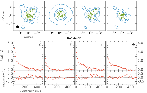
Figure 2: Images and visibilities of data preparation steps for IRAS 4A-SE. Top: imaged data; bottom: binned real and imaginary visibilities. From left to right: a) raw data, b) envelope model, c) raw data with envelope subtracted, d) raw data with envelope and companion subtracted. The contours start at 3$\sigma$, then in steps of 7$\sigma$ until 31$\sigma,$ and then in steps of 31$\sigma$, where $\sigma$=10 mJy (5 mJy for envelope model image).

1. A spherically symmetric model of the envelope is constructed. The model is subtracted from the observational visibilities (see Sect. 3.1 for details).

2. A Gaussian and a point source are fitted to all components and those corresponding to companion(s) are subtracted from the visibilities. Visual inspection of the residual image confirms the success of the subtraction.

3. The phase center is shifted so that the continuum peak of the source of interest is at the center (relevant for companion systems).

At this point, the visibility data of all sources consist primarily of emission not reproducible with the spherical envelope models and free of resolved close companion sources. IRAS 4A-SE/NW and VLA 1623 A both have nearby companions that are resolved and need to be subtracted. IRAS 4B has a weak companion at $\sim 10$″ directly east, but due to its weak nature and distance from the main source it should not contribute any real flux; however, it was subtracted before analysis. For IRAS 4A, where both sources have been analyzed and are relatively strong, there is a risk of left-over structure from the subtracted companion. However, the spatial scales involved in the fitting are smaller than the separation, and thus any structure left over should not affect the results.

The structure remaining after the envelope subtraction is assumed to be flattened and inclined with respect to the plane of the sky. Since the Gaussian and power-law disk models assume a face-on viewing angle when calculating the visibilities (circular Gaussian and face-on disk) the observational data need to be de-projected to be aligned with the plane of the sky. Since the minimization is done on the observations subtracted by the model, it is easier to de-project the data rather than the model. To de-project the model more calculation steps need to be performed to compare it with the observations because they need to be compared in the same $\mathit{u}$-$\mathit{v}$ coordinates, which change when the visibilities are de-projected (see Appendix B.2). Assuming that the remaining compact axisymmetric structure is aligned approximately perpendicular to the large-scale outflow, the visibilities can be de-projected using the best estimates of the position angle (PA, measured east of north) and inclination. A face-on disk has an inclination of 0^∘ and an edge-on disk 90^∘. Subsequently, the real amplitudes of the visibilities are analyzed, first by fitting an intensity distribution consisting of a circular Gaussian together with a point source. This provides an estimate of the radius and a mass of the compact structure. The estimate of the radius is then used in the fitting of the physical power-law disk model as the disk radius ($r_{c}$). The models are fitted to the data using the Levenberg-Marquardt algorithm through the SciPy.optimize module (Jones et al. 2001).

The de-projection is performed on the visibilities using the same approach as given in Hughes et al. (2007), some details are given in Appendix B.2. If there are previous estimates of the PA and inclination (e.g., from gas tracers showing rotation) these values are used. Otherwise it is assumed that $\mathrm{PA}_{\mathrm{disk}}=\mathrm{PA}_{\mathrm{outflow}}+90^{\circ}$. Furthermore, for all sources except VLA 1623 A and IRAS 2A, there are no reliable estimates for the inclination angle, which is then assumed to be $60^{\circ}$. However, changes in the inclination of 15^∘ are run to assess the effects of inclination (45^∘and 75^∘). Current best estimates of the PA and inclination from literature, where applicable, are listed in Table 3. We note that inclinations close to edge-on, i.e., 90^∘ are not easily constrained with this method ($\lim\limits_{i\to 90}\cos^{-1}i\to\infty$).

Table 3: Adopted position angle and inclination of compact component.

Source	PAdisk	inc	Ref.
IRAS 2A	$110^{\circ}$	$58.5^{\circ}\pm 15$	1
IRAS 4A-SE/NW	$100^{\circ}$	$60^{\circ}\pm 15$	2
IRAS 4B	$90^{\circ}$	$60^{\circ}\pm 15$	2
VLA 1623	$35^{\circ}\pm 5$	$55^{\circ}\pm 5$	3

4 Results

4.1 Gaussian intensity distribution

The results of fitting a Gaussian intensity distribution plus point source are shown in Figure 3. The parameters of the best fits are presented in Table 4. The radius is calculated from 0.42 $\times\theta_{\rm FWHM}$.

In fitting a point source it is assumed that the most compact structure is not resolved. The data of IRAS 2A and IRAS 4A-SE/-NW are represented well by the fit function. However, for these sources information on the longest baselines, as available for VLA 1623 A and IRAS 4B, is missing. Furthermore, the data for IRAS 4A-NW/-SE have a lower signal-to-noise ratio. IRAS 4B has a jump in real amplitude around 280 $k\lambda$; the reason for this is unclear. Toward the longest baselines, the IRAS 4B amplitude seems to go below zero, signifying that perhaps the compact structure has a sharp edge or that the center of mass is slightly offset from the phase center; longer baseline data could shed light on this. For VLA 1623 A, the non-zero values out to long $\mathit{u}$-$\mathit{v}$ distances show that a compact structure is probably present. The Gaussian plus point source fit is worse in the range $70\sim 250$ $k\lambda$ for VLA 1623 A.

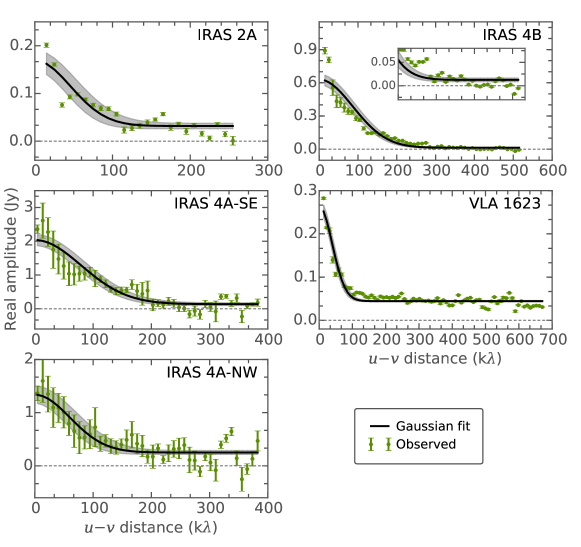
Figure 3: Best-fit Gaussian model with added point source where applicable. The green points are the envelope subtracted and de-projected data with the variance from the binning as uncertainty, while the black line and gray area show the best fit and the 1$\sigma$ region (changing the fitted parameters by $\pm$1$\sigma$).

Table 4: Parameters from Gaussian fits, with uncertainty in the values reflecting changes in inclination by $15^{\circ}$.

Source	$F_{G}$	$\theta_{\mathrm{FWHM}}$		$F_{\mathrm{PS}}$	$R$ (=$r_{c}$)	$M_{\mathrm{gas}}$
	[mJy]	[$\arcsec$]	[AU]	[mJy]	[AU]	[$\times 10^{-3}M_{\odot}$]
IRAS 2A	$140$$\begin{subarray}{c}+40\\ -20\end{subarray}$	$1.7$$\begin{subarray}{c}+0.6\\ -0.2\end{subarray}$	$396$$\begin{subarray}{c}+150\\ -50\end{subarray}$	$30\pm 10$	$167$$\begin{subarray}{c}+63\\ -21\end{subarray}$	$155$$\begin{subarray}{c}+46\\ -27\end{subarray}$
IRAS 4B	$600$$\begin{subarray}{c}+60\\ -40\end{subarray}$	$0.9\pm 0.1$	$210\pm 15$	$\leq 10$	$88\pm 6$	$556$$\begin{subarray}{c}+55\\ -46\end{subarray}$
IRAS 4A-SE	$1900\pm 100$	$0.98$$\begin{subarray}{c}+0.32\\ -0.26\end{subarray}$	$230$$\begin{subarray}{c}+75\\ -60\end{subarray}$	$100$$\begin{subarray}{c}+100\\ -60\end{subarray}$	$96$$\begin{subarray}{c}+32\\ -25\end{subarray}$	$262$$\begin{subarray}{c}+26\\ -21\end{subarray}$
VLA 1623	$220\pm 16$	$2.0$$\begin{subarray}{c}+0.9\\ -0.4\end{subarray}$	$237$$\begin{subarray}{c}+105\\ -46\end{subarray}$	$40\pm 2$	$100$$\begin{subarray}{c}+44\\ -20\end{subarray}$	$54\pm 4$
IRAS 4A-NW	$1100\pm 160$	$1.3$$\begin{subarray}{c}+0.2\\ -0.1\end{subarray}$	$303$$\begin{subarray}{c}+92\\ -41\end{subarray}$	$300$$\begin{subarray}{c}+40\\ -100\end{subarray}$	$127\pm 18$	$183$$\begin{subarray}{c}+26\\ -34\end{subarray}$

4.2 Power-law disk

The resulting best-fit power-law disk model to the envelope subtracted and de-projected real visibility amplitude curves for each source are presented in Figure 4. The best-fit parameters are summarized in Table 5. For $r_{c}$, the best-fit value from the Gaussian fit is taken. We note that the power-law disk fits the temperature multiplied with the density, i.e., $p+q$, with $q$ fixed to 0.5 before fitting $\Sigma$ and $p$. The density fall-off in the taper is significantly steeper and this is reflected in the increase in intensity in the visibilities. The values for the density power-law index, $p$ is similar for all sources ($\sim 1$) except IRAS 4B. The gas surface density varies between 2.4 and 51 g cm^-2 at $r_{0}=50$ AU.

IRAS 2A and IRAS 4A-NW/-SE are well represented with the disk model, with similar constraints on the disk parameters. The fit is worse in the range $70\sim 200$ $k\lambda$ for VLA 1623 A and IRAS 4B. This is partly because of the addition of a taper, whose radial density decrease depends on the disk density (i.e., $2-p$). While not ideal, it should not have a significant effect on the estimated disk parameters and the subsequent discussion on the derived physical conditions.

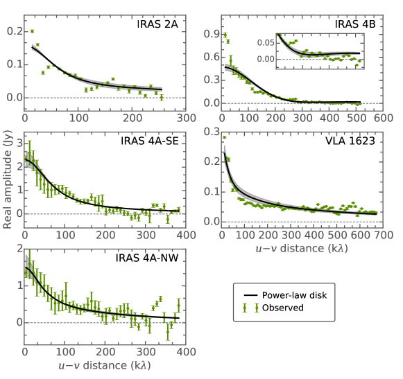
Figure 4: Resulting best-fit power-law disk for the sources. The green points are the envelope subtracted and de-projected data with the variance from the binning as uncertainty, while the black line and gray area show the best fit and the 1$\sigma$ region (changing the fitted parameters by $\pm$1$\sigma$).

The corresponding best-fit density and temperature as a function of radius for each source are shown in Figures 5 and 6. The largest jump in density between the disk and envelope is seen in IRAS 4B where the interface between them is not smooth. The disk derived for IRAS 4B is small and has a shallow density profile. As noted, the vertical disk structure is not fitted in this study, so the mid-plane disk density connects with the envelope through the taper. The continuum $\tau=1$ radius at 1.5 mm lies within $R\sim 10$ AU for all sources and will not affect our results for the larger scales.

The midplane temperature profile does not align well with the envelope for IRAS 2A (Fig. 6), but does merge smoothly for the other sources. Disk shadowing will affect both temperature and density, for example, lowering the temperature just behind the disk, which could explain the jump in temperature and density in some of the disk-envelope interfaces shown here (e.g., Murillo et al. 2015). It is important to note again here that the midplane gas volume density is derived using a combination of fitted and fixed parameters and it should be kept in mind when interpreting the results. The midplane density depends on the scale height, which is a function of the temperature profile (which is fixed, see Sect. 3.3).

Table 5: Parameters from power-law disk fitting; the ranges reflect changes in the assumed $r_{\mathrm{c}}$, inclination, and PA from the fitting of a Gaussian and point source (see section 4.1).

Source	$p$	$\Sigma_{0}$	$M_{\mathrm{disk}}$	min($T>100$ K)
		[g cm-2]	[$\times 10^{-3}M_{\odot}$]	%
IRAS 2A	$0.8$$\begin{subarray}{c}+0.4\\ -0.2\end{subarray}$	$6.7$$\begin{subarray}{c}+1.2\\ -0.4\end{subarray}$	$42$$\begin{subarray}{c}+9\\ -5\end{subarray}$	$9$$\begin{subarray}{c}+6\\ -3\end{subarray}$
IRAS 4B	$\leq 0.1$$\begin{subarray}{c}+1.1\\ -\end{subarray}$	$51$$\begin{subarray}{c}+15\\ -5\end{subarray}$	$140$$\begin{subarray}{c}+105\\ -15\end{subarray}$	$7.4$$\begin{subarray}{c}+26\\ -0.3\end{subarray}$
IRAS 4A-SE	$1.0\pm 0.1$	$26\pm 3$	$90$$\begin{subarray}{c}+34\\ -20\end{subarray}$	$25$$\begin{subarray}{c}+12\\ -6\end{subarray}$
VLA 1623	$1.2\pm 0.2$	$2.4\pm 0.5$	$9\pm 1$	$30\pm 3$
IRAS 4A-NW	$1.1$$\begin{subarray}{c}+0.1\\ -0.2\end{subarray}$	$11.3$$\begin{subarray}{c}+2\\ -1.2\end{subarray}$	$52$$\begin{subarray}{c}+11\\ -4\end{subarray}$	$22$$\begin{subarray}{c}+1\\ -2\end{subarray}$

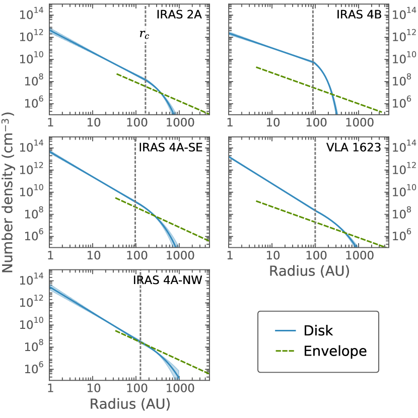
Figure 5: Midplane gas volume density of the disk (blue) and the envelope (dashed green) as a function of radius. The blue shaded area shows the uncertainty in the number density varying parameters $\pm 1\sigma$. The volume density at the disk surface is a factor of $e^{-\nicefrac{{1}}{{2}}}\sim 0.6$ lower.

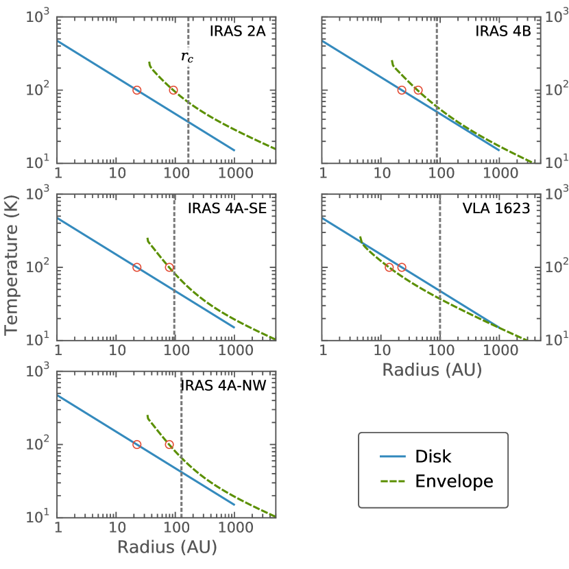
Figure 6: Midplane temperature of the disk (blue) and the envelope (dashed green). The red circles mark where $T=100$ K and the vertical dashed line indicates the radius of the compact component ($r_{c}$).

5 Discussion

In this study, the de-projected continuum interferometric visibilities of five deeply embedded low-mass protostars are fitted with two different models, a Gaussian disk intensity distribution and a parametrized analytical expression of a vertically isothermal thin disk model. Before fitting the disk models, the current best model of the surrounding large-scale envelope and possible companion sources were subtracted.

5.1 Method uncertainties

There are various uncertainties related to the analysis which should be re-iterated before an in-depth discussion of the results.

The analyzed envelope subtracted residual visibilities depend on the envelope model used. The most recent models by Kristensen et al. (2012) and Jørgensen et al. (2002) are used to minimize this source of uncertainty. The models use both the observed SED and radial profile of the millimeter emission to constrain the envelope density and temperature profile.

The disk mass estimate, Equation (3), assumes an average temperature of the disk, which is the same for all sources. For simple cases this should be a good enough approximation, and facilitates easy comparison with results from other studies of the same or similar sources where the same method was used.

The assumed stellar mass and temperature profile of the power-law disk will affect the derived midplane density, and to some extent the surface density profile (i.e., $p$) given the degeneracies of calculating the visibilities (i.e., $p+q$ is fitted). The effect of the stellar mass on the derived midplane density is small. The assumed temperature profile also affects the midplane density, in the opposite way from mass. Increasing both the stellar mass and disk temperature by a factor of two will not have any effect on the derived midplane density. However, the assumed temperature profile has an impact on the amount of material above 100 K and thus the derived molecular abundances. As discussed in Sect. 3.3 we have assumed a temperature profile that is reasonable and in agreement with other studies. Future higher sensitivity and higher resolution observations of molecular lines sensitive to the temperature structure can potentially improve the constraints.

5.2 Disk radii and masses

The derived range of radii of the disk-like structures, $90-170$ AU, are plausible and are marginally resolved in these data sets. The disk diameter ($2{\times}r_{c}$) corresponds to the scale where there is a sharp increase in flux.

For the one source, VLA 1623 A, for which the radius of the Keplerian disk has been determined from kinematics of C¹⁸O line emission, a value of $R=150$ AU (rotationally supported to $R=180$ AU) has been found by Murillo et al. (2013b). The radius derived in this study is $r_{c}=100^{+44}_{-20}$ AU, which is somewhat smaller but in agreement within the uncertainties. In more mature disks, the mm dust continuum has been found to be more centrally concentrated than the gas due to radial drift (e.g., Andrews et al. 2012). This could be happening in VLA 1623 even at this early stage.

The inferred masses vary between the sources, and are different depending on the method. The mass estimates using the Gaussian intensity distribution are generally higher ($54-556\times 10^{-3}$ $M_{\rm\sun}$) than for the power-law disks ($9-140\times 10^{-3}$ $M_{\rm\sun}$). While the mass estimates for the power-law disk use the fitted disk parameters put into Equation (8), the mass from the Gaussian intensity distribution is simply the Gaussian with the point source flux added put into Equation (3).

Jørgensen et al. (2005b) fitted a Gaussian intensity distribution together with a point source to 350 GHz SMA continuum observations of IRAS 2A covering baselines between 18 and 164 $k\lambda$. They found a radius of this compact emission of $100-200$ AU and a mass of 0.1 $M_{\rm\sun}$ (for $T_{\mathrm{avg}}=30$ K and flux of $\mathit{u}$-$\mathit{v}$ dist $>50$ $k\lambda$). Our disk radius and mass derived from the Gaussian intensity distribution agree with this estimate.

In IRAS 4B the relatively high mass derived with the power-law disk shows a small disk with a flat density distribution and a high surface density. Choi & Lee (2011) argue from the extent of the 1.3 cm continuum emission toward IRAS 4B that the radius of the compact disk-like structure is $R=25$ AU, roughly 1/3 of the disk size derived here. Larger grains, similar to those responsible for the emission at these wavelengths, are affected by radial drift to a higher extent (e.g., Birnstiel et al. 2010), and the cm emission is thus expected to be more compact, in agreement with these results. However, Choi et al. (2010) derived a radius of at least 220 AU from kinematic analysis of ammonia emission at 24 GHz (1.3 cm).

Jørgensen et al. (2009) estimated the mass of the compact components toward IRAS 2A ($56\times 10^{-3}$ $M_{\rm\sun}$), IRAS 4A-SE ($460\times 10^{-3}$ $M_{\rm\sun}$) and IRAS 4B ($240\times 10^{-3}$ $M_{\rm\sun}$). This was done by using a combination of the interferometric flux on 50 $k\lambda$ scales and single-dish flux at 850 $\mu$m. The masses derived from the power-law disk in this study agree for IRAS 2A and within a factor of 2 for IRAS 4B, but the disk mass derived for IRAS 4A-SE is five times lower. The gas masses derived from the Gaussian intensity distribution are about a factor of 2-3 higher than that of Jørgensen et al. for IRAS 2A and IRAS 4B, but for IRAS 4A-SE it is roughly half. The generally higher masses derived using the Gaussian intensity distribution comes from the fact that Jørgensen et al. uses the flux at 50 $k\lambda$ to derive the disk mass and a steeper power-law envelope profile; Fig. 3 shows that this flux is still not the total flux of the compact component left after subtracting the spherically symmetric envelope contribution.

The fitted density power laws show that there is a significant amount of material at large radii. This is important for fragmentation. Numerical studies have shown that if the ratio of disk to stellar mass ($M_{\mathrm{disk}}/M_{*}$) goes above $\sim 0.25$ the disk can be prone to gravitational instabilities (e.g., Lodato & Rice 2004; Dong et al. 2015). It has been suggested that any gravitational instabilities may induce the formation of multiple star systems (e.g., Kratter et al. 2010). These instabilities can only form in disks more massive than in the Class II stage (i.e., higher $M_{disk}/M_{*}$), thus more likely in the earlier protostellar stages when the stellar mass is still low. Given that about half of all solar analogs are found in multiple systems (Raghavan et al. 2010), determining the physical conditions in the early stages of disk formation is of great importance for the understanding of the formation of multiple star and planetary systems. For VLA 1623, where the stellar mass was determined previously, the $M_{\mathrm{disk}}/M_{*}$ ratio is $0.009/0.20=0.045$, indicating a gravitationally stable disk. All the other sources have values higher than $M_{\mathrm{disk}}/M_{*}=0.25$, assuming $M_{*}=0.05$. With $M_{*}=0.2$ as for VLA 1623, the disks have ratios close to or higher than $0.25$, indicating that the disks may be gravitationally unstable even in this scenario.

For all sources, the envelope is relatively well characterized on large scales, since both radial profiles and the SED were used to model the large-scale envelope. It is not clear whether the added taper, which is frequently used in similar studies for more evolved disks (i.e., Class II disks) (Andrews & Williams 2008), is a good representation of the disk-to-envelope interface for these sources. However, it is also important to characterize this interface region that is not fitted by spherical envelope models. For some of the sources in the study there are no observations with longer baseline coverage, thus adding degeneracy to the fitting

It is clear from the various data sets used here that it is important to cover longer $\mathit{u}$-$\mathit{v}$ distances to constrain the disk. Of all the observations, only the ALMA data on VLA 1623 A cover baselines that fully resolve the disk-like structure, the observations of the other sources should still be sensitive to the structure but to a less extent. For more robust models of the radial structure, higher resolution observations are needed.

5.3 Envelope-only model

Recently, Maury et al. (2014) fitted the 1.3 mm continuum visibility amplitudes of IRAS 2A obtained with PdBI (baselines 14 to 557 $k\lambda$, 8″-0$\aas@@fstack{\prime\prime}$35) with a power-law intensity distribution, representing a single spherical envelope. The intensity as a function of $\mathit{u}$-$\mathit{v}$ distance for an envelope with $T\propto{r^{-q}}$ and $\rho\propto{r^{-p}}$ is $V\propto{b^{a}}$, where $a=(p+q-3)$. To compare to these results, such a power-law envelope was fitted to the visibilities of IRAS 2A in this study. It is important to note that the two companions that Maury et al. subtract prior to envelope-fitting do not exist in our data (see Sect. 2 for references), so we do not subtract any companion sources for this analysis.

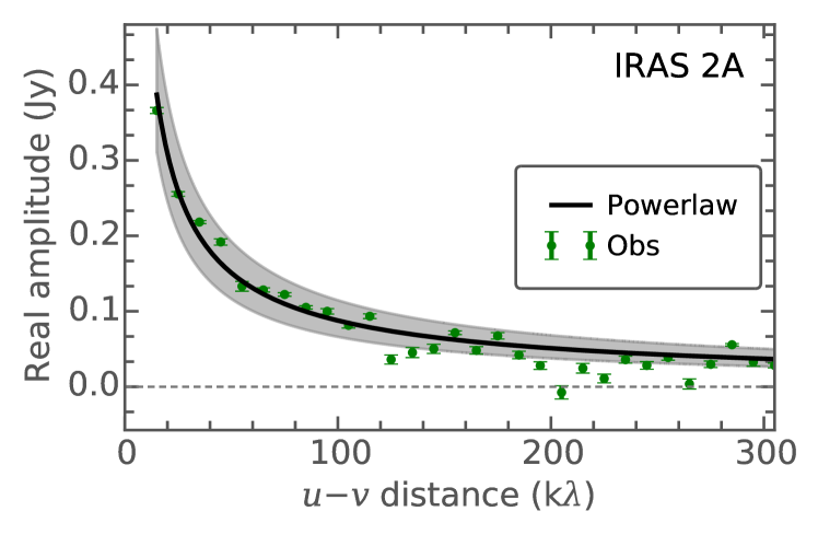
Figure 7: IRAS 2A envelope power-law model, $V=Cb^{a}$, applied to the IRAS 2A data without subtraction of our envelope model. Here $a=-0.78\pm 0.03$, $C=3.2\pm 0.4$, and $b$ is in units of k$\lambda$.

The resulting power-law envelope fit is shown in Fig. 7, and the fit coefficients are $a=-0.78\pm 0.03$ ($V=C{b^{a}}$, where $C=3.2\pm 0.4$ if $b$ is in k$\lambda$). This implies $p+q=2.22$, and for comparison, Maury et al. presented $a=-0.45\pm 0.05$, i.e., $p+q=2.55$. The envelope-only power-law fits for the rest of the sources in this study are presented in Appendix 18 and Table 7.

While the modified power-law envelope model can reproduce the interferometric visibilities, it does not mean that the entire envelope is reproduced with this model alone. Modifying the envelope model by Kristensen et al. to fit the visibility amplitudes gives the results shown in Fig. 8. The model that best reproduces the interferometric visibility amplitude is where the volume number density is increased by a factor of 5 from $4.9\times 10^{8}$ to $25\times 10^{8}$ cm^-3 and the power law steepened from $p=-1.7$ to $-2.0$. This essentially represents moving more of the mass inward to accommodate the flux on longer baselines, i.e., smaller scales. The wiggles at large baselines are due to the sharp edge introduced at the inner radius.

With this modified model the analytical prediction of the temperature slope ($q$) from the single powerlaw envelope fit of Maury et al. would be $2.55-2.0=0.55$. The resulting temperature profile from TRANSPHERE is roughly approximated by $q=0.5$. This shows that the modified model of the envelope is consistent with that of Maury et al. on these aspects.

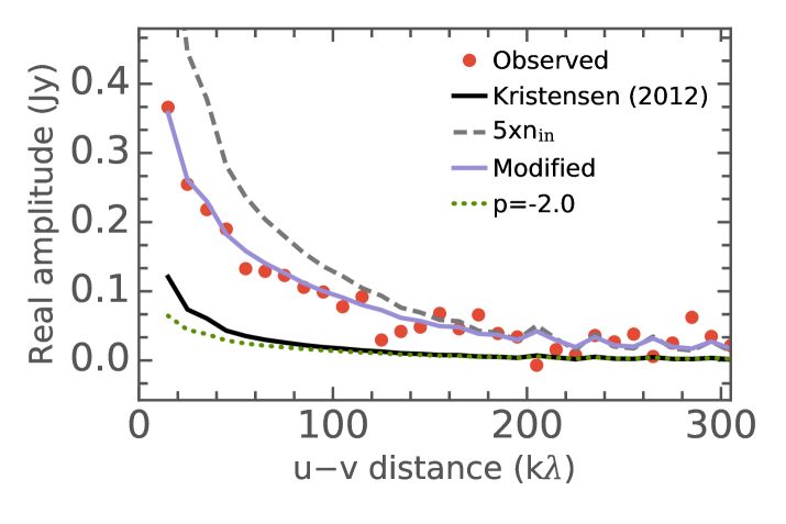
Figure 8: Modified envelope-only models from Kristensen et al. (2012) in comparison to the observed interferometric visibilities of IRAS 2A. The non-modified model of Kristensen et al. is shown as a black line; the by eye best-fitting modified model, with $5\times$ higher number density ($n_{\mathrm{in}}$) at the inner radius and $p=-2.0$ is shown in purple.

The observed flux at 219 GHz given by Maury et al. (2014) (scaled from Motte & André 2001), is 0.86 Jy. The total flux at 219 GHz after convolving with the 11″ beam is 1.02 Jy for the Kristensen et al. model and 1.25 Jy for the modified interferometric model. Given a typical absolute flux uncertainty in single-dish observations of about 20%, the modified model is higher by $45\%$, while the Kristensen et al. model is higher by $19\%$. The modified model is higher by a significant amount, although not enough to discard it. Thus the modified single power-law envelope can reproduce the interferometric visibilities and almost the total flux.

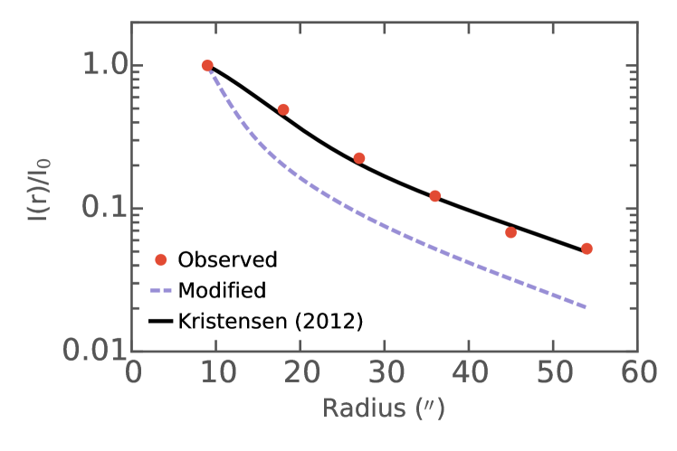
Figure 9: Radial profile at 850 $\mu$m for IRAS 2A (red dots, FWHM${}_{\mathrm{beam}}=$ 19$\aas@@fstack{\prime\prime}$5) with the power-law envelope model of Kristensen et al. (2012) (black line), and the modified Kristensen et al. model (purple dashes, $5\times n_{\mathrm{in}}$ and $p=-2.0$).

The envelope models of Kristensen et al. and Jørgensen et al. (2002) are not only constrained by the total flux (SED), but also by the radial profile of the large-scale emission. The radial profiles of the two envelope models are shown in Fig. 9 together with observations at 850 $\mu$m for IRAS 2A.

While the model of Kristensen et al. fits the radial profile, on scales larger than about 20″ the modified model is at least 5 times lower than the observations. This is not surprising since much of the mass has been moved inward to fit the compact component of the emission. Thus, the single power-law envelope cannot reproduce the interferometric visibilities and the large-scale emission at the same time. Additionally, the morphology of IRAS 2A shows non-circular symmetric structures already at scales of 2″ in 1.3mm observations (Tobin et al. 2015b), demonstrating that simply modifying the inner radial density distribution of the power-law envelope is not enough. Thus, a compact structure, possibly disk-like, together with an extended envelope provides the best fit to the total observed emission.

5.4 Mass above 100 K

The percentage of the material that is above 100 K for each radius of the disk is computed based on the best-fit power-law disk model. Figure 10 presents the mass enclosed for each radius compared with the mass where $T\geq 100$ K. The radius where $T=100$ K is the same for all sources, given the assumption that $q=0.5$ and a fixed $r_{T_{0}}$ (effectively fixed $L_{*}$). The different sizes and densities of the disk then change the percentage of the warm material at a certain radius. The $\sim 20\%$ limit lies between $50\sim 150$ AU for the sources except for VLA 1623 A, which never goes below 30%. In Table 5 the percentage at the disk radius ($r_{c}$) is listed for the studied sources. The percentage can be relatively large, up to 30% (VLA 1623 A) and as low as 7% (IRAS 4A-SE). Changing the temperature structure such that the 100 K radius is at 5 AU but leaving everything else the same lowers the percentage to 9% for VLA 1623 A and to 0.5% for IRAS 4A-SE.

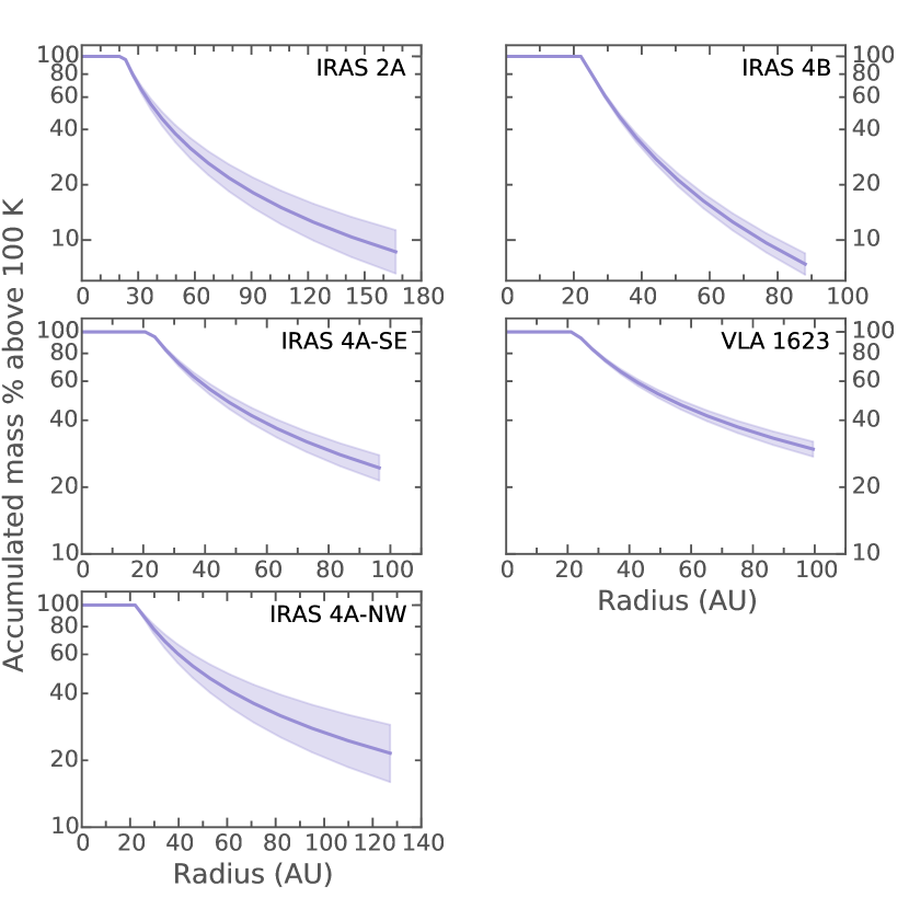
Figure 10: Percentage of cumulative mass that is above 100 K as a function of radius for the sources studied. The shaded area reflects the mass introduced by the uncertainty in the fitted disk parameters with $\pm 1\sigma$ ( i.e., $\Sigma,p$).

5.5 Water abundance

As mentioned in the introduction, the assumed physical structure affects the abundance estimates. The amount of material with dust temperatures above $\sim 100$ K is particularly important since this is the temperature above which water ice sublimates and any complex molecules locked into the ice are released (Fraser et al. 2001) (the specific temperature depends on density, see Harsono et al. 2015).

Persson et al. (2012) estimate gas phase water abundances to total (cold+warm) H₂ densities for four of the sources observed in this study by using masses derived by Jørgensen et al. (2009) from the 850 $\mu$m continuum in the same beam. In Fig. 11 these values, and new estimates derived using the masses from this study are shown. The largest difference is seen for IRAS 4B and the upper limit of IRAS 4A-SE. With the new total disk/compact masses the warm-water abundance is slightly different. However, it is expected that the whole structure will not have temperatures above 100 K, thus the fractional abundance using the total mass inferred from the power-law and Gaussian disk can be seen as a lower limit to the relative gas phase abundance of water.

Correcting for the amount of material in the disk above 100 K increases the fractional abundances with up to almost two orders of magnitude. However, as shown by Harsono et al. (2015), part of the warm water emission could originate in the envelope surrounding the disk, i.e., the hot corino, thus making the fractional abundances for $T>100$ K material upper limits. This part of the model is not captured in the modeling of the disk, which focuses on the cold dense region. We note that the power-law disk model does not include any vertical structure. A temperature gradient along the vertical direction of the disk could increase the amount of warm gas ($T>100$ K), thus decreasing the abundance of gas phase water.

Given the models used in this study, correcting for the material with $T>100$ K gives relative water abundances as high as $6.2\times 10^{-5}$ for IRAS 2A, comparable to what is expected from sublimated ices ($10^{-4}$). For the rest of the sources studied, the same abundances are lower by $1\sim 3$ orders of magnitude from this high value in IRAS 2A. The disk in IRAS 4B is compact and dense (flat profile and high surface density), this causes the very low relative abundance of water. The envelope power-law is also flatter than the other sources. These results show that disks are not as dry as previously stated, but are not “wet” either.

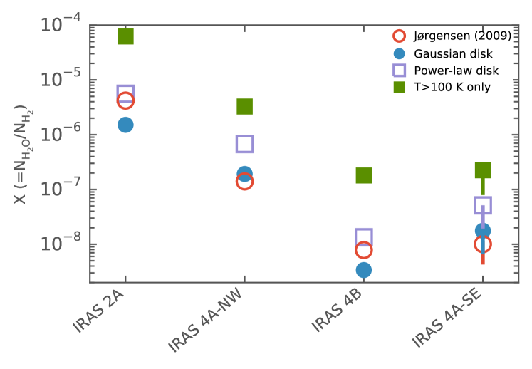
Figure 11: Relative abundance of gas-phase water derived from observations of p-H${}_{2}^{18}$O by (Persson et al. 2012) and continuum (for estimating the H₂ abundance) for different methods of estimating the disk gas mass. The values of the mass by Jørgensen et al. (2009) used by Persson et al. (2012) are drawn as red open circles. The size of the symbols reflects the uncertainty; for IRAS 4A-SE the values are upper-limits.

Table 6: Derived relative water abundance ($\times 10^{-7}$) for the various models shown in Fig. 11. A corresponds to abundance derived from Jørgensen et al. (2009) (red open circle, Fig. 11), B from the Gaussian disk derived in this study (blue filled circle), C from the power-law disk (open purple square), and D from material in the power-law disk with only with T¿100 K (green filled square).

Source	A	B	C	D
IRAS 2A	$42$	$15$	$56$	$620$
IRAS 4A-NW	$1.4$	$2$	$6.76$	$33$
IRAS 4B	$0.1$	$0.03$	$0.1$	$1.8$
IRAS 4A-SE	$<0.1$	$<0.2$	$<0.5$	$<2$

6 Summary and outlook

The deeply embedded nature of Class 0 sources adds to the difficulty of determining the physical structure on small, sub-300 AU, scales. Several parameters need to be determined. On small scales, a thin-disk model can approximate the emission and make it possible to constrain the radial density profile, assuming a fixed temperature distribution. For the five Class 0 sources studied here, the derived disk radii are similar ($90-170$ AU), and masses from fitting a power-law disk range from $9-140\times 10^{-3}$ $M_{\rm\sun}$. Most of the derived power-law disk masses agree with previous estimates using other methods. The gas surface density varies between $2.4-51$ g cm^-2 (at $r_{0}=50$ AU). The temperature and density profiles have a smooth transition to the envelope in general.

The inferred disk/compact masses are high, comparable to or higher than the assumed stellar mass of 0.05 $M_{\rm\sun}$. VLA 1623 is the only source in this study where a stellar mass of 0.2 $M_{\rm\sun}$ has been determined. The ratio between the disk and stellar mass determines when disk instabilities may develop. At ratios higher than 0.25 the disk becomes prone to gravitational instabilities (e.g., Lodato & Rice 2004; Dong et al. 2015), which would apply to most of our disks up to $M_{*}\approx 0.3$$M_{\rm\sun}$.

The fractional amount of material above 100 K in the whole disk varies between $9-30$ %, with an assumed temperature profile of $q=0.5$ (see Sect. 3.3 for choice of $q$). A lower $q$ would increase the percentages, and a higher $q$ decrease. The main assumption is that the compact structure is indeed a disk that can be described with this power-law model. Using previous observations of p-H${}_{2}^{18}$O, we estimate relative gas phase water abundances to total H₂ densities and for H₂ warmer than 100 K. The relative water abundance in the warm gas ($>$100 K) of these disks are $6.2\times 10^{-5}$ (IRAS 2A), $0.33\times 10^{-5}$ (IRAS 4A-NW), $1.8\times 10^{-8}$ (IRAS 4B), and $<2\times 10^{-8}$ (IRAS 4A-SE). Thus, the gas-phase water abundance can be as high as the expected value for sublimated ice of $10^{-4}$ (as in IRAS 2A), but are lower for the other sources studied.

The techniques developed here can be applied to large samples of sources. The next step is to image both the continuum and molecular line tracers at higher angular resolution with ALMA and with good $uv$ coverage on all scales to constrain any disk-like structure as well as the transition to the larger scale envelope.

Appendix A Output from the various analysis steps

The output (image, real, and imaginary visibility amplitude) of each step of the data preparation, i.e., envelope and companion subtraction, are shown in Figures 12 to 14. In each figure, the raw data, envelope model, envelope subtracted data, and companion subtracted data are shown. For VLA 1623 A the companion subtraction makes a clear difference, which can be seen even in the visibilities.

Figure 12: Images and visibilities of data preparation steps for IRAS 2A. From left to right: raw data, envelope model, raw data with envelope subtracted. The images start at 3$\sigma$, in steps of 3$\sigma$ until 9$\sigma$ where it is in steps of 9$\sigma$, $\sigma$=1.6 mJy ($\sigma$=0.2 mJy for envelope model image).

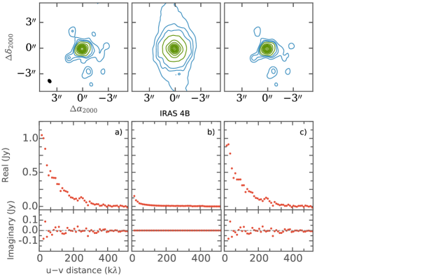
Figure 13: Images and visibilities of data preparation steps for IRAS 4B. From left to right: raw data, envelope model, raw data with envelope subtracted. The images start at 3$\sigma$, in steps of 3$\sigma$ until 15$\sigma$ where it is in steps of 15$\sigma$, $\sigma$=2 mJy ($\sigma$=0.13 mJy for envelope model image). As pointed out in the text, the observations of IRAS 4B are dynamic range limited, which causes the compact emission around the main continuum peak seen in the images above; these are convolution artifacts and are not real.

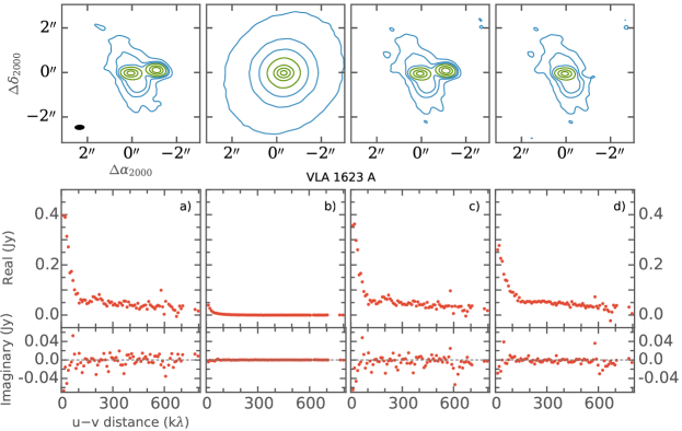
Figure 14: Images and visibilities of data preparation steps for VLA 1623 A. Top: imaged data; bottom: binned real and imaginary visibilities. From left to right; a) raw data, b) envelope model, c) raw data with envelope subtracted, d) raw data with envelope and companion subtracted. The contours start at 3$\sigma$ then insteps of 7$\sigma$ until 30$\sigma$ and then in steps of 30$\sigma$, $\sigma$=0.6 mJy (0.02 mJy for envelope model image).

Appendix B Working with visibilities

B.1 Binning visibilities - vector averaging

The visibilities are binned in annuli around the origin of the $\mathit{u}$-$\mathit{v}$ plane. In the following equations, $N_{p}$ is the number of points in the bin, $re_{i}$ the real part of each visibility, and $Re$ the binned real amplitude in each bin; the same notation holds for $im_{i}$ and $Im$:

$$Re=\dfrac{\sum^{N_{p}}_{i=0}re_{i}}{N_{p}};Im=\dfrac{\sum^{N_{p}}_{i=0}im_{i}}{N_{p}}$$ (12)

$$\sigma_{Re}=\sqrt{\dfrac{\sum_{i=0}^{N_{p}}re^{2}_{i}-N_{p}Re^{2}}{N_{p}-1}};\sigma_{Im}=\sqrt{\dfrac{\sum_{i=0}^{N_{p}}im^{2}_{i}-N_{p}Im^{2}}{N_{p}-1}}$$ (13)

The combined amplitude is simply the square root of the sum of the squared real and imaginary amplitudes (i.e., $A=\sqrt{Re^{2}+Im^{2}}$), the standard deviation is then the error propagation of the individual errors of the real and imaginary parts.

$$\sigma_{A}=\sqrt{\dfrac{\left(\dfrac{Re\sigma_{Re}}{A}\right)^{2}+\left(\dfrac{Im\sigma_{Im}}{A}\right)^{2}}{N_{p}-2}}$$ (14)

B.2 Rotation and inclination

Each u and v coordinate is rotated $PA$ degrees and inclined $i$ degrees. This is accomplished by first calculating the $\mathit{u}$-$\mathit{v}$ distances from the origin

$$r_{uv}=\sqrt{u^{2}+v^{2}}$$ (15)

and the angle of the new point by subtracting the position angle from the current direction of the point (measured east of north):

$$\gamma=\arctan\left(\frac{v}{u}\right)-PA.$$ (16)

Calculating the rotated and inclined (along the rotated u-axis) coordinate system, we get new u and v coordinates

$$u^{\prime}=r_{uv}\sin\gamma\cos i$$ (17)

$$v^{\prime}=r_{uv}\sin\gamma$$ (18)

with the new $\mathit{u}$-$\mathit{v}$ distance naturally given by $r^{\prime}_{uv}=\sqrt{u^{\prime 2}+v^{\prime 2}}$.

Appendix C Envelope-only results

This section presents the results of the envelope-only fitting of the interferometric visibilities. As shown in Section 5, these models do not necessarily fit the large-scale emission. For IRAS 4A-SE two fits were performed, one including all visibilities and one with only visibilties with $\mathit{u}$-$\mathit{v}$ distances shorter than 150 $k\lambda$ to minimize interference from the binary source.

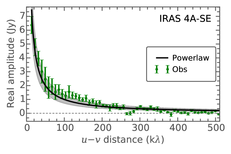
Figure 15: Power-law envelope model fit to IRAS 4A-SE data. All the $\mathit{u}$-$\mathit{v}$ distances were fit.

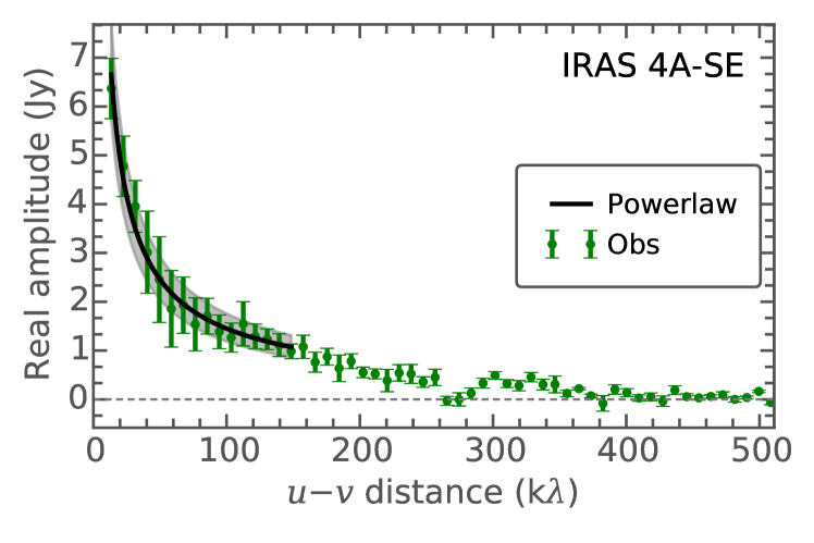
Figure 16: Power-law envelope model fit to IRAS 4A-SE data. Only $\mathit{u}$-$\mathit{v}$ distances shorter than 150 $k\lambda$ were fit to make sure the model is not contaminated by the companion source. The parameters for the fit are $C=48\pm 4$ and $a=-0.76\pm 0.02$.

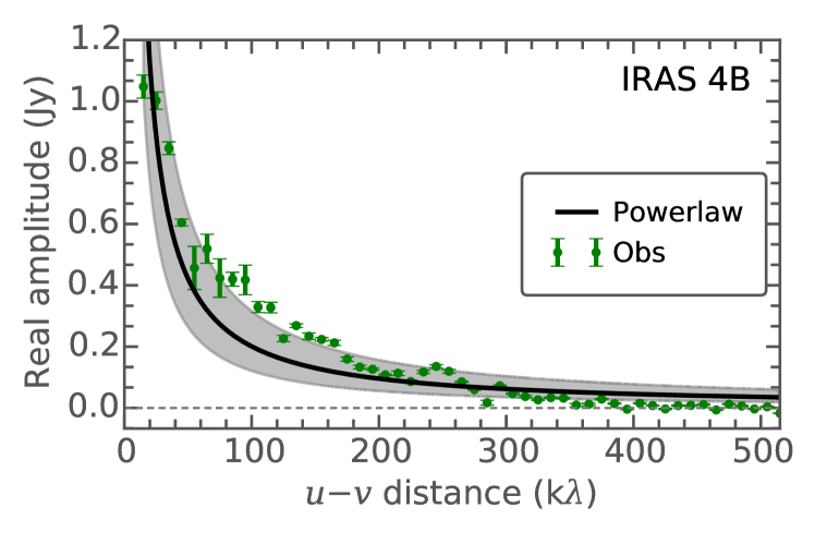
Figure 17: Power-law envelope model fit to IRAS 4B.

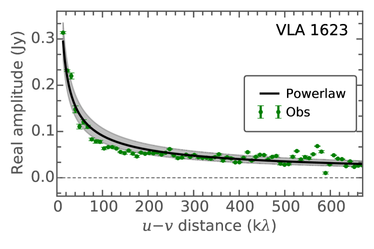
Figure 18: Power-law envelope model fit to VLA 1623.

Table 7: Parameters for the envelope-only models from a fit $V(b)=Cb^{a}$.

Source	$C$	$a$
IRAS 2A	$3.2\pm 0.4$	$-0.78\pm 0.03$
IRAS 4B	$28\pm 6$	$-1.07\pm 0.05$
IRAS 4A-SE	$102\pm 15$	$-1.01\pm 0.04$
VLA 1623	$1.4\pm 0.1$	$-0.59\pm 0.02$

Appendix D Envelope parameters

Table 8: Parameters used for the envelope models.

Source	$p_{\mathrm{env}}$	$r_{\mathrm{in}}$ [AU]	$r_{\mathrm{out}}$ [AU]	$n_{\mathrm{in}}$ (cm-3)
IRAS 2A	1.7	35.9	17950	$4.9\times 10^{8}$
IRAS 4A	1.8	33.5	33500	$3.1\times 10^{9}$
IRAS 4B	1.4	15.0	12000	$2.0\times 10^{9}$
VLA 1623	1.4	4.3	10320	$1.6\times 10^{9}$