Clique decompositions of multipartite graphs and completion of Latin squares

Abstract.

Our main result essentially reduces the problem of finding an edge-decomposition of a balanced $r$-partite graph of large minimum degree into $r$-cliques to the problem of finding a fractional $r$-clique decomposition or an approximate one. Together with very recent results of Bowditch and Dukes as well as Montgomery on fractional decompositions into triangles and cliques respectively, this gives the best known bounds on the minimum degree which ensures an edge-decomposition of an $r$-partite graph into $r$-cliques (subject to trivially necessary divisibility conditions). The case of triangles translates into the setting of partially completed Latin squares and more generally the case of $r$-cliques translates into the setting of partially completed mutually orthogonal Latin squares.

1. Introduction

A $K_{r}$-decomposition of a graph $G$ is a partition of its edge set $E(G)$ into cliques of order $r$. If $G$ has a $K_{r}$-decomposition, then certainly $e(G)$ is divisible by $\binom{r}{2}$ and the degree of every vertex is divisible by $r-1$. A classical result of Kirkman [19] asserts that, when $r=3$, these two conditions ensure that $K_{n}$ has a triangle decomposition (i.e. Steiner triple systems exist). This was generalized to arbitrary $r$ (for large $n$) by Wilson [29] and to hypergraphs by Keevash [17]. Recently, there has been much progress in extending this from decompositions of complete host graphs to decompositions of graphs which are allowed to be far from complete (see the final paragraphs in Section 1.1). In this paper, we investigate this question in the $r$-partite setting. This is of particular interest as it implies results on the completion of partial Latin squares and more generally partial mutually orthogonal Latin squares.

1.1. Clique decompositions of $r$-partite graphs

Our main result (Theorem 1.1) states that if $G$ is (i) balanced $r$-partite, (ii) satisfies the necessary divisibility conditions and (iii) its minimum degree is at least a little larger than the minimum degree which guarantees an approximate decomposition into $r$-cliques, then $G$ in fact has a decomposition into $r$-cliques. (Here an approximate decomposition is a set of edge-disjoint copies of $K_{r}$ which cover almost all edges of $G$.) To state this result precisely, we need the following definitions.

We say that a graph or multigraph $G$ on $(V_{1},\dots,V_{r})$ is $K_{r}$-divisible if $G$ is $r$-partite with vertex classes $V_{1},\dots,V_{r}$ and for all $1\leq j_{1},j_{2}\leq r$ and every $v\in V(G)\setminus(V_{j_{1}}\cup V_{j_{2}})$,

$$d(v,V_{j_{1}})=d(v,V_{j_{2}}).$$

Note that in this case, for all $1\leq j_{1},j_{2},j_{3},j_{4}\leq r$ with $j_{1}\neq j_{2}$, $j_{3}\neq j_{4}$, we automatically have $e(V_{j_{1}},V_{j_{2}})=e(V_{j_{3}},V_{j_{4}})$. In particular, $e(G)$ is divisible by $e(K_{r})=\binom{r}{2}$.

Let $G$ be an $r$-partite graph on $(V_{1},\dots,V_{r})$ with $|V_{1}|=\dots=|V_{r}|=n$. Let

$$\hat{\delta}(G):=\min\{d(v,V_{j}):1\leq j\leq r,\;v\in V(G)\setminus V_{j}\}.$$

An $\eta$-approximate $K_{r}$-decomposition of $G$ is a set of edge-disjoint copies of $K_{r}$ covering all but at most $\eta n^{2}$ edges of $G$. We define $\hat{\delta}^{\eta}_{K_{r}}(n)$ to be the infimum over all $\delta$ such that every $K_{r}$-divisible graph $G$ on $(V_{1},\dots,V_{r})$ with $|V_{1}|=\dots=|V_{r}|=n$ and $\hat{\delta}(G)\geq\delta n$ has an $\eta$-approximate $K_{r}$-decomposition. Let $\hat{\delta}^{\eta}_{K_{r}}:=\limsup_{n\rightarrow\infty}\hat{\delta}^{\eta}_{K_{r}}(n)$. So if ${\varepsilon}>0$ and $G$ is sufficiently large, $K_{r}$-divisible and $\hat{\delta}(G)>(\hat{\delta}^{\eta}_{K_{r}}+{\varepsilon})n$, then $G$ has an $\eta$-approximate $K_{r}$-decomposition. Note that it is important here that $G$ is $K_{r}$-divisible. Take, for example, the complete $r$-partite graph with vertex classes of size $n$ and remove $\lceil\eta n\rceil$ edge-disjoint perfect matchings between one pair of vertex classes. The resulting graph $G$ satisfies $\hat{\delta}(G)=n-\lceil\eta n\rceil$, yet has no $\eta$-approximate $K_{r}$-decomposition whenever $r\geq 3$.

Theorem 1.1.

For every $r\geq 3$ and every ${\varepsilon}>0$ there exists an $n_{0}\in\mathbb{N}$ and an $\eta>0$ such that the following holds for all $n\geq n_{0}$. Suppose $G$ is a $K_{r}$-divisible graph on $(V_{1},\dots,V_{r})$ with $|V_{1}|=\dots=|V_{r}|=n$. If $\hat{\delta}(G)\geq(\hat{\delta}^{\eta}_{K_{r}}+{\varepsilon})n$, then $G$ has a $K_{r}$-decomposition.

By a result of Haxell and Rödl [15], the existence of an approximate decomposition follows from that of a fractional decomposition. So together with very recent results of Bowditch and Dukes [5] as well as Montgomery [22] on fractional decompositions into triangles and cliques respectively, Theorem 1.1 implies the following explicit bounds. We discuss this derivation in Section 1.3.

Theorem 1.2.

For every $r\geq 3$ and every ${\varepsilon}>0$ there exists an $n_{0}\in\mathbb{N}$ such that the following holds for all $n\geq n_{0}$. Suppose $G$ is a $K_{r}$-divisible graph on $(V_{1},\dots,V_{r})$ with $|V_{1}|=\dots=|V_{r}|=n$.

• If $r=3$ and $\hat{\delta}(G)\geq\left(\frac{24}{25}+{\varepsilon}\right)n$, then $G$ has a $K_{3}$-decomposition.

• If $r\geq 4$ and $\hat{\delta}(G)\geq\left(1-\frac{1}{10^{6}r^{3}}+{\varepsilon}\right)n$, then $G$ has a $K_{r}$-decomposition.

If $G$ is the complete $r$-partite graph, this corresponds to a theorem of Chowla, Erdős and Straus [7]. A bound of $(1-1/(10^{16}r^{29}))n$ was claimed by Gustavsson [14]. The following conjecture seems natural (and is implicit in [14]).

Conjecture 1.3.

For every $r\geq 3$ there exists an $n_{0}\in\mathbb{N}$ such that the following holds for all $n\geq n_{0}$. Suppose $G$ is a $K_{r}$-divisible graph on $(V_{1},\dots,V_{r})$ with $|V_{1}|=\dots=|V_{r}|=n$. If $\hat{\delta}(G)\geq(1-1/(r+1))n$, then $G$ has a $K_{r}$-decomposition.

A construction which matches the lower bound in Conjecture 1.3 is described in Section 3.1 (this construction also gives a similar lower bound on $\hat{\delta}^{\eta}_{K_{r}}$). In the non-partite setting, the triangle case is a long-standing conjecture by Nash-Williams [23] that every graph $G$ on $n$ vertices with minimum degree at least $3n/4$ has a triangle decomposition (subject to divisibility conditions). Barber, Kühn, Lo and Osthus [3] recently reduced its asymptotic version to proving an approximate or fractional version. Corresponding results on fractional triangle decompositions were proved by Yuster [30], Dukes [10], Garaschuk [11] and Dross [9].

More generally [3] also gives results for arbitrary graphs, and corresponding fractional decomposition results have been obtained by Yuster [30], Dukes [10] as well as Barber, Kühn, Lo, Montgomery and Osthus [2]. Further results on $F$-decompositions of non-partite graphs (leading on from [3]) have been obtained by Glock, Kühn, Lo, Montgomery and Osthus [12]. Amongst others, for any bipartite graph $F$, they asymptotically determine the minimum degree threshold which guarantees an $F$-decomposition. Finally, Glock, Kühn, Lo and Osthus [13] gave a new (combinatorial) proof of the existence of designs. The results in [13] generalize those in [17], in particular, they imply a resilience version and a decomposition result for hypergraphs of large minimum degree.

1.2. Mutually orthogonal Latin squares and $K_{r}$-decompositions of $r$-partite graphs

A Latin square $\mathcal{T}$ of order $n$ is an $n\times n$ grid of cells, each containing a symbol from $[n]$, such that no symbol appears twice in any row or column. It is easy to see that $\mathcal{T}$ corresponds to a $K_{3}$-decomposition of the complete tripartite graph $K_{n,n,n}$ with vertex classes consisting of the rows, columns and symbols.

Now suppose that we have a partial Latin square; that is, a partially filled in grid of cells satisfying the conditions defining a Latin square. When can it be completed to a Latin square? This natural question has received much attention. For example, a classical theorem of Smetaniuk [25] as well as Anderson and Hilton [1] states that this is always possible if at most $n-1$ entries have been made (this bound is best possible). The case $r=3$ of Conjecture 1.3 implies that, provided we have used each row, column and symbol at most $n/4$ times, it should also still be possible to complete a partial Latin square. This was conjectured by Daykin and Häggkvist [8]. (For a discussion of constructions which match this conjectured bound, see Wanless [28].) Note that the conjecture of Daykin and Häggkvist corresponds to the special case of Conjecture 1.3 when $r=3$ and the condition of $G$ being $K_{r}$-divisible is replaced by that of $G$ being obtained from $K_{n,n,n}$ by deleting edge-disjoint triangles.

More generally, we say that two Latin squares $R$ (red) and $B$ (blue) drawn in the same $n\times n$ grid of cells are orthogonal if no two cells contain the same combination of red symbol and blue symbol. In the same way that a Latin square corresponds to a $K_{3}$-decomposition of $K_{n,n,n}$, a pair of orthogonal Latin squares corresponds to a $K_{4}$-decomposition of $K_{n,n,n,n}$ where the vertex classes are rows, columns, red symbols and blue symbols. More generally, there is a natural bijection between sequences of $r-2$ mutually orthogonal Latin squares (where every pair from the sequence are orthogonal) and $K_{r}$-decompositions of complete $r$-partite graphs with vertex classes of equal size. Sequences of mutually orthogonal Latin squares are also known as transversal designs. Theorem 1.2 can be used to show the following (see Section 3.2 for details).

Theorem 1.4.

For every $r\geq 3$ and every ${\varepsilon}>0$ there exists an $n_{0}\in\mathbb{N}$ such that the following holds for all $n\geq n_{0}$. Let

$$c_{r}:=\begin{cases}\frac{1}{25}&\text{if}\ r=3,\\ \frac{9}{10^{7}r^{3}}&\text{if}\ r\geq 4.\end{cases}$$

Let $\mathcal{T}_{1},\dots,\mathcal{T}_{r-2}$ be a sequence of mutually orthogonal partial $n\times n$ Latin squares (drawn in the same $n\times n$ grid). Suppose that each row and each column of the grid contains at most $(c_{r}-{\varepsilon})n$ non-empty cells and each coloured symbol is used at most $(c_{r}-{\varepsilon})n$ times. Then $\mathcal{T}_{1},\dots,\mathcal{T}_{r-2}$ can be completed to a sequence of mutually orthogonal Latin squares.

Here, by a non-empty cell we mean a cell containing at least one symbol (in at least one of the colours). The best previous bound for the triangle case $r=3$ is due to Bartlett [4], who obtained a minimum degree bound of $(1-10^{-4})n$. This improved an earlier bound of Chetwynd and Häggkvist [6] as well as the one claimed by Gustavsson [14]. We are not aware of any previous upper or lower bounds for $r\geq 4$.

1.3. Fractional and approximate decompositions

A fractional $K_{r}$-decomposition of a graph $G$ is a non-negative weighting of the copies of $K_{r}$ in $G$ such that the total weight of all the copies of $K_{r}$ containing any fixed edge of $G$ is exactly $1$. Fractional decompositions are of particular interest to us because of the following result of Haxell and Rödl, of which we state only a very special case (see [31] for a shorter proof).

Theorem 1.5 (Haxell and Rödl [15]).

For every $r\geq 3$ and every $\eta>0$ there exists an $n_{0}\in\mathbb{N}$ such that the following holds. Let $G$ be a graph on $n\geq n_{0}$ vertices that has a fractional $K_{r}$-decomposition. Then $G$ has an $\eta$-approximate $K_{r}$-decomposition.

We define $\hat{\delta}^{*}_{K_{r}}(n)$ to be the infimum over all $\delta$ such that every $K_{r}$-divisible graph $G$ on $(V_{1},\dots,V_{r})$ with $|V_{1}|=\dots=|V_{r}|=n$ and $\hat{\delta}(G)\geq\delta n$ has a fractional $K_{r}$-decomposition. Let $\hat{\delta}^{*}_{K_{r}}:=\limsup_{n\rightarrow\infty}\hat{\delta}^{*}_{K_{r}}(n)$. Theorem 1.5 implies that, for every $\eta>0$, $\hat{\delta}^{\eta}_{K_{r}}\leq\hat{\delta}^{*}_{K_{r}}$. Together with Theorem 1.1, this yields the following.

Corollary 1.6.

For every $r\geq 3$ and every ${\varepsilon}>0$ there exists an $n_{0}\in\mathbb{N}$ such that the following holds for all $n\geq n_{0}$. Suppose $G$ is a $K_{r}$-divisible graph on $(V_{1},\dots,V_{r})$ with $|V_{1}|=\dots=|V_{r}|=n$. If $\hat{\delta}(G)\geq(\hat{\delta}^{*}_{K_{r}}+{\varepsilon})n$, then $G$ has a $K_{r}$-decomposition.

In particular, to prove Conjecture 1.3 asymptotically, it suffices to show that $\hat{\delta}^{*}_{K_{r}}\leq 1-1/(r+1)$. Similarly, improved bounds on $\hat{\delta}^{*}_{K_{r}}$ would lead to improved bounds in Theorem 1.4 (see Corollary 3.2).

For triangles, the best bound on the ‘fractional decomposition threshold’ is due to Bowditch and Dukes [5].

Theorem 1.7 (Bowditch and Dukes [5]).

$\hat{\delta}^{*}_{K_{3}}\leq\frac{24}{25}$.

For arbitrary cliques, Montgomery obtained the following bound. Somewhat weaker bounds (obtained by different methods) are also proved in [5].

Theorem 1.8 (Montgomery [22]).

For every $r\geq 3$, $\hat{\delta}^{*}_{K_{r}}\leq 1-\frac{1}{10^{6}r^{3}}$.

Note that together with Corollary 1.6, these results immediately imply Theorem 1.2.

This paper is organised as follows. In Section 2 we introduce some notation and tools which will be used throughout this paper. In Section 3 we give extremal constructions which support the bounds in Conjecture 1.3 and we provide a proof of Theorem 1.4. Section 4 outlines the proof of Theorem 1.1 and guides the reader through the remaining sections in this paper.

2. Notation and tools

Let $G$ be a graph and let $\mathcal{P}=\{U^{1},\dots,U^{k}\}$ be a partition of $V(G)$. We write $G[U^{1}]$ for the subgraph of $G$ induced by $U^{1}$ and $G[U^{1},U^{2}]$ for the bipartite subgraph of $G$ induced by the vertex classes $U^{1}$ and $U^{2}$. We will also sometimes write $G[U^{1},U^{1}]$ for $G[U^{1}]$. We write $G[\mathcal{P}]:=G[U^{1},\dots,U^{k}]$ for the $k$-partite subgraph of $G$ induced by the partition $\mathcal{P}$. We write $U^{<i}$ for $U^{1}\cup\dots\cup U^{i-1}$. We say the partition $\mathcal{P}$ is equitable if its parts differ in size by at most one. Given a set $U\subseteq V(G)$, we write $\mathcal{P}[U]$ for the restriction of $\mathcal{P}$ to $U$.

Let $G$ be a graph and let $U,V\subseteq V(G)$. We write $N_{G}(U,V):=\{v\in V:xv\in E(G)\text{ for all }x\in U\}$ and $d_{G}(U,V):=|N_{G}(U,V)|$. For $v\in V(G)$, we write $N_{G}(v,V)$ for $N_{G}(\{v\},V)$ and $d_{G}(v,V)$ for $d_{G}(\{v\},V)$. If $U$ and $V$ are disjoint, we let $e_{G}(U,V):=e(G[U,V])$.

Let $G$ and $H$ be graphs. We write $G-H$ for the graph with vertex set $V(G)$ and edge set $E(G)\setminus E(H)$. We write $G\setminus H$ for the subgraph of $G$ induced by the vertex set $V(G)\setminus V(H)$. We call a vertex-disjoint collection of copies of $H$ in $G$ an $H$-matching. If the $H$-matching covers all vertices in $G$, we say that it is perfect.

Throughout this paper, we consider a partition $V_{1},\dots,V_{r}$ of a vertex set $V$ such that $|V_{j}|=n$ for all $1\leq j\leq r$. Given a set $U\subseteq V$, we write

$$U_{j}:=U\cap V_{j}.$$

A $k$-partition of $V$ is a partition $\mathcal{P}=\{U^{1},\dots,U^{k}\}$ of $V$ such that the following hold:

1. for each $1\leq j\leq r$, $\{U^{i}_{j}:1\leq i\leq k\}$ is an equitable partition of $V_{j}$;

2. for each $1\leq i\leq k$, $|U^{i}_{1}|=\dots=|U^{i}_{r}|$.

If $G$ is an $r$-partite graph on $(V_{1},\dots,V_{r})$, we sometimes also refer to a $k$-partition of $G$ (instead of a $k$-partition of $V(G)$). We write $K_{r}(k)$ for the complete $r$-partite graph with vertex classes of size $k$. We say that an $r$-partite graph $G$ on $(V_{1},\dots,V_{r})$ is balanced if $|V_{1}|=\dots=|V_{r}|$.

We use the symbol $\ll$ to denote hierarchies of constants, for example $1/n\ll a\ll b<1$, where the constants are chosen from right to left. The notation $a\ll b$ means that there exists an increasing function $f$ for which the result holds whenever $a\leq f(b)$.

Let $m,n,N\in\mathbb{N}$ with $m,n<N$. The hypergeometric distribution with parameters $N$, $n$ and $m$ is the distribution of the random variable $X$ defined as follows. Let $S$ be a random subset of $\{1,2,\dots,N\}$ of size $n$ and let $X:=|S\cap\{1,2,\dots,m\}|$. We will frequently use the following bounds, which are simple forms of Hoeffding’s inequality.

Lemma 2.1 (see [16, Remark 2.5 and Theorem 2.10]).

Let $X\sim B(n,p)$ or let $X$ have a hypergeometric distribution with parameters $N,n,m$. Then $\mathbb{P}(|X-\mathbb{E}(X)|\geq t)\leq 2e^{-2t^{2}/n}$.

Lemma 2.2 (see [16, Corollary 2.3 and Theorem 2.10]).

Suppose that $X$ has binomial or hypergeometric distribution and $0<a<3/2$. Then $\mathbb{P}(|X-\mathbb{E}(X)|\geq a\mathbb{E}(X))\leq 2e^{-a^{2}\mathbb{E}(X)/3}$.

3. Extremal graphs and completion of Latin squares

3.1. Extremal graphs

The following proposition shows that the minimum degree bound conjectured in Conjecture 1.3 would be best possible. It also provides a lower bound on the approximate decomposition threshold $\hat{\delta}^{\eta}_{K_{r}}$ (and thus on the fractional decomposition threshold $\hat{\delta}^{*}_{K_{r}}$).

Proposition 3.1.

Let $r\in\mathbb{N}$ with $r\geq 3$ and let $\eta>0$. For infinitely many $n$, there exists a $K_{r}$-divisible graph $G$ on $(V_{1},\dots,V_{r})$ with $|V_{1}|=\dots=|V_{r}|=n$ and $\hat{\delta}(G)=\lceil(1-1/(r+1))n\rceil-1$ which does not have a $K_{r}$-decomposition. Moreover, $\hat{\delta}^{\eta}_{K_{r}}\geq 1-1/(r+1)-\eta$.

Proof. Let $m\in\mathbb{N}$ with $1/m\ll\eta$ and let $n:=(r-1)m$. Let $\{U^{1},\dots,U^{r-1}\}$ be a partition of $V_{1}\cup\dots\cup V_{r}$ such that, for each $1\leq i\leq r-1$ and each $1\leq j\leq r$, $U^{i}_{j}=U^{i}\cap V_{j}$ has size $m$.

Let $G_{0}$ be the intersection of the complete $r$-partite graph on $(V_{1},\ldots,V_{r})$ and the complete $(r-1)$-partite graph on $(U^{1},\ldots,U^{r-1})$. For each $1\leq q\leq m$ and each $1\leq i\leq r-1$, let $H^{i}_{q}$ be a graph formed by starting with the empty graph on $U^{i}$ and including a $q$-regular bipartite graph with vertex classes $(U^{i}_{j_{1}},U^{i}_{j_{2}})$ for each $1\leq j_{1}<j_{2}\leq r$. Let $H_{q}:=H^{1}_{q}\cup\cdots\cup H^{r-1}_{q}$ and let $G_{q}:=G_{0}\cup H_{q}$. Observe that $G_{q}$ is regular, $K_{r}$-divisible and

$$\hat{\delta}(G_{q})=(r-2)m+q.$$

Now $G_{0}$ is $(r-1)$-partite, so every copy of $K_{r}$ in $G_{q}$ contains at least one edge of $H_{q}$. Therefore, any collection of edge-disjoint copies of $K_{r}$ in $G$ will leave at least

$$\ell(G_{q}):=e(G_{q})-e(H_{q})\binom{r}{2} =\big{(}(r-2)m+q-\binom{r}{2}q\big{)}\binom{r}{2}n$$

$$=(m-(r+1)q/2)(r-2)\binom{r}{2}n$$

edges of $G_{q}$ uncovered. Let $q_{0}:=\lceil 2m/(r+1)\rceil-1$. Then $\ell(G_{q_{0}})>0$, so $G_{q_{0}}$ does not have a $K_{r}$-decomposition. Also,

$$\hat{\delta}(G_{q_{0}})=(r-2)m+\lceil 2m/(r+1)\rceil-1=\lceil(1-1/(r+1))n\rceil-1.$$

Now let $q_{\eta}:=\lceil 2m/(r+1)-\eta n\rceil$. We have $\hat{\delta}(G_{q_{\eta}})\geq(1-1/(r+1)-\eta)n$ and

$$\ell(G_{q_{\eta}}) \geq(m-(2m/(r+1)-\eta n+1)(r+1)/2)(r-2)\binom{r}{2}n$$

$$=(\eta n-1)(r+1)(r-2)r(r-1)n/4\geq 6(\eta n-1)n>\eta n^{2}.$$

Thus, $\hat{\delta}^{\eta}_{K_{r}}\geq 1-1/(r+1)-\eta$.        $\square$

3.2. Completion of mutually orthogonal Latin squares

In this section, we give a proof of Theorem 1.4. We also discuss how better bounds on the fractional decomposition threshold would immediately lead to better bounds on $c_{r}$. For any $r$-partite graph $H$ on $(V_{1},\dots,V_{r})$, we let $\overline{H}$ denote the $r$-partite complement of $H$ on $(V_{1},\dots,V_{r})$.

Proof of Theorem 1.4. By making ${\varepsilon}$ smaller if necessary, we may assume that ${\varepsilon}\ll 1$. Let $n_{0}\in\mathbb{N}$ be such that $1/n_{0}\ll{\varepsilon},1/r$. Use $\mathcal{T}_{1},\dots,\mathcal{T}_{r-2}$ to construct a balanced $r$-partite graph $G$ with vertex classes $V_{j}=[n]$ for $1\leq j\leq r$ as follows. For each $1\leq i,j,k\leq n$ and each $1\leq m\leq r-2$, if in $\mathcal{T}_{m}$ the cell $(i,j)$ contains the symbol $k$, include a $K_{3}$ on the vertices $i\in V_{r-1}$, $j\in V_{r}$ and $k\in V_{m}$. (If the cell $(i,j)$ is filled in different $\mathcal{T}_{m}$, this leads to multiple edges between $i\in V_{r-1}$ and $j\in V_{r}$, which we disregard.) For each $1\leq i,j,k,k^{\prime}\leq n$ and each $1\leq m<m^{\prime}\leq r-2$ such that the cell $(i,j)$ contains symbol $k$ in $\mathcal{T}_{m}$ and symbol $k^{\prime}$ in $\mathcal{T}_{m^{\prime}}$, add an edge between the vertices $k\in V_{m}$ and $k^{\prime}\in V_{m^{\prime}}$.

If $r=3$, then $G$ is an edge-disjoint union of copies of $K_{3}$, so $G$ is $K_{3}$-divisible. Then $\overline{G}$ is also $K_{3}$-divisible and $\hat{\delta}(\overline{G})\geq(24/25+{\varepsilon})n$. So we can apply Theorem 1.2 to find a $K_{3}$-decomposition of $\overline{G}$ which we can then use to complete $\mathcal{T}_{1}$ to a Latin square.

Suppose now that $r\geq 4$. Observe that $G$ consists of an edge-disjoint union of cliques $H_{1},\dots,H_{q}$ such that, for each $1\leq i\leq q$, $H_{i}$ contains an edge of the form $xy$ where $x\in V_{r-1}$ and $y\in V_{r}$. We have $q\leq(c_{r}-{\varepsilon})n^{2}$. We now show that we can extend $G$ to a graph of small maximum degree which can be decomposed into $q$ copies of $K_{r}$. We will do this by greedily extending each $H_{i}$ in turn to a copy $H_{i}^{\prime}$ of $K_{r}$. Suppose that $1\leq p\leq q$ and we have already found edge-disjoint $H_{1}^{\prime},\dots,H_{p-1}^{\prime}$. Given $v\in V(G)$, let $s(v,p-1)$ be the number of graphs in $\{H_{1}^{\prime},\dots,H_{p-1}^{\prime}\}\cup\{H_{p},\dots,H_{q}\}$ which contain $v$. Suppose inductively that $s(v,p-1)\leq 10(c_{r}-{\varepsilon}^{2})n/9$ for all $v\in V(G)$. (This holds when $p=1$ by our assumption that each row and each column of the grid contains at most $(c_{r}-{\varepsilon})n$ non-empty cells and each coloured symbol is used at most $(c_{r}-{\varepsilon})n$ times.) For each $1\leq j\leq r$, let $B_{j}:=\{v\in V_{j}:s(v,p-1)\geq 10(c_{r}-{\varepsilon})n/9\}$. We have

(3.1) $$|B_{j}|\leq\frac{q}{10(c_{r}-{\varepsilon})n/9}\leq\frac{9n}{10}.$$

Let $G_{p-1}:=G\cup\bigcup_{i=1}^{p-1}(H_{i}^{\prime}-H_{i})$. Note that

(3.2) $$\hat{\delta}(\overline{G}_{p-1})\geq(1-10(c_{r}-{\varepsilon}^{2})/9)n,$$

by our inductive assumption. We will extend $H_{p}$ to a copy of $K_{r}$ as follows. Let $\{j_{1},\dots,j_{m}\}=\{j:1\leq j\leq r\text{ and }V(H_{p})\cap V_{j}=\emptyset\}$. For each $j_{i}$ in turn, starting with $j_{1}$, choose one vertex $x_{j_{i}}$ from the set $N_{\overline{G}_{p-1}}(V(H_{p})\cup\{x_{j_{1}},\dots,x_{j_{i-1}}\},V_{j_{i}}\setminus B_{j_{i}})$. This is possible since (3.1) and (3.2) imply

$$d_{\overline{G}_{p-1}}(V(H_{p})\cup\{x_{j_{1}},\dots,x_{j_{i-1}}\},V_{j_{i}}\setminus B_{j_{i}})\geq(1/10-(r-1)10(c_{r}-{\varepsilon}^{2})/9)n>0.$$

Let $H_{p}^{\prime}$ be the copy of $K_{r}$ with vertex set $V(H_{p})\cup\{x_{j}:1\leq j\leq r\text{ and }V(H_{p})\cap V_{j}=\emptyset\}$. By construction, for every $v\in V(G)$, the number $s(v,p)$ of graphs in $\{H_{1}^{\prime},\dots,H_{p}^{\prime}\}\cup\{H_{p+1},\dots,H_{q}\}$ which contain $v$ satisfies $s(v,p)\leq 10(c_{r}-{\varepsilon}^{2})n/9$.

Continue in this way to find edge-disjoint $H_{1}^{\prime},\dots,H_{q}^{\prime}$ such that $s(v,q)\leq 10(c_{r}-{\varepsilon}^{2})n/9$. Let $G_{q}:=\bigcup_{1\leq i\leq q}H_{i}^{\prime}$. We have $\hat{\delta}(\overline{G}_{q})\geq(1-10(c_{r}-{\varepsilon}^{2})/9)n=(1-1/10^{6}r^{3}+10{\varepsilon}^{2}/9)n$ and, since $G_{q}$ is an edge-disjoint union of copies of $K_{r}$, we know that $\overline{G}_{q}$ is $K_{r}$-divisible. So we can apply Theorem 1.2 to find a $K_{r}$-decomposition $\mathcal{F}$ of $\overline{G}_{q}$. Note that $\mathcal{F}^{\prime}:=\mathcal{F}\cup\bigcup_{1\leq i\leq q}H_{i}^{\prime}$ is a $K_{r}$-decomposition of the complete $r$-partite graph. Since $H_{i}\subseteq H_{i}^{\prime}$ for each $1\leq i\leq q$, we can use $\mathcal{F}^{\prime}$ to complete $\mathcal{T}_{1},\dots,\mathcal{T}_{r-2}$ to a sequence of mutually orthogonal Latin squares.        $\square$

The proof of Theorem 1.4 also shows how better bounds for the fractional decomposition threshold $\hat{\delta}^{*}_{K_{r}}$ lead to better bounds on $c_{r}$. More precisely, by replacing the ‘10/9’ in the above inductive upper bound on $s(v,p-1)$ by ‘2’ and making the obvious adjustments to the calculations we obtain the following result.

Corollary 3.2.

For all $r\geq 3$ and $n\in\mathbb{N}$, define $\beta_{r}(n)$ to be the supremum over all $\beta$ so that the following holds: Let $\mathcal{T}_{1},\dots,\mathcal{T}_{r-2}$ be a sequence of mutually orthogonal partial $n\times n$ Latin squares (drawn in the same $n\times n$ grid). Suppose that each row and each column of the grid contains at most $\beta n$ non-empty cells and each coloured symbol is used at most $\beta n$ times. Then $\mathcal{T}_{1},\dots,\mathcal{T}_{r-2}$ can be completed to a sequence of mutually orthogonal Latin squares.

Let $\beta_{r}:=\liminf_{n\to\infty}\beta_{r}(n)/n$. Also, for every $r\geq 3$, let

$$\beta^{\prime}_{r}:=\begin{cases}1-\hat{\delta}^{*}_{K_{3}}&\text{if}\ r=3,\\ (1-\hat{\delta}^{*}_{K_{r}})/4&\text{if}\ r\geq 4.\end{cases}$$

Then $\beta_{r}\geq\beta_{r}^{\prime}$.

If, in addition, we know that, for each $1\leq i,j\leq n$, the entry $(i,j)$ of the grid is either filled by a symbol of every colour or it is empty, we can omit the factor $4$ in the definition of $\beta^{\prime}_{r}$ for each $r\geq 4$. We obtain this stronger result since the graph $G$ obtained from $\mathcal{T}_{1},\dots,\mathcal{T}_{r-2}$ will automatically be $K_{r}$-decomposable.

4. Proof Sketch

Our proof of Theorem 1.1 builds on the proof of the main results of [3], but requires significant new ideas. In particular, the $r$-partite setting involves a stronger notion of divisibility (the non-partite setting simply requires that $r-1$ divides the degree of each vertex of $G$ and that $\binom{r}{2}$ divides $e(G)$) and we have to work much harder to preserve it during our proof. This necessitates a delicate ‘balancing’ argument (see Section 10). In addition, we use a new construction for our absorbers, which allows us to obtain the best possible version of Theorem 1.1. (The construction of [3] would only achieve $1-1/3(r-1)$ in place of $1-1/(r+1)$.)

The idea behind the proof is as follows. We are assuming that we have access to a black box approximate decomposition result: given a $K_{r}$-divisible graph $G$ on vertex classes of size $n$ with $\hat{\delta}(G)\geq(\hat{\delta}^{\eta}_{K_{r}}+{\varepsilon})n$ we can obtain an approximate $K_{r}$-decomposition that leaves only $\eta n^{2}$ edges uncovered. We would like to obtain an exact decomposition by ‘absorbing’ this small remainder. By an absorber for a $K_{r}$-divisible graph $H$ we mean a graph $A_{H}$ such that both $A_{H}$ and $A_{H}\cup H$ have a $K_{r}$-decomposition. For any fixed $H$ we can construct an absorber $A_{H}$. But there are far too many possibilities for the remainder $H$ to allow us to reserve individual absorbers for each in advance.

To bridge the gap between the output of the approximate result and the capabilities of our absorbers, we use an iterative absorption approach (see also [3] and [20]). Our guiding principle is that, since we have no control on the remainder if we apply the approximate decomposition result all in one go, we should apply it more carefully. More precisely, we begin by partitioning $V(G)$ at random into a large number of parts $U^{1},\ldots,U^{k}$. Since $k$ is large, $G[U^{1},\ldots,U^{k}]$ still has high minimum degree, and, since the partition is random, each $G[U^{i}]$ also has high minimum degree. We first reserve a sparse and well structured subgraph $J$ of $G[U^{1},\ldots,U^{k}]$, then we obtain an approximate decomposition of $G[U^{1},\ldots,U^{k}]-J$ leaving a sparse remainder $H$. We then use a small number of edges from the $G[U^{i}]$ to cover all edges of $H\cup J$ by copies of $K_{r}$. Let $G^{\prime}$ be the subgraph of $G$ consisting of those edges not yet used in the approximate decomposition. Then all edges of $G^{\prime}$ lie in some $G^{\prime}[U^{i}]$, and each $G^{\prime}[U^{i}]$ has high minimum degree, so we can repeat this argument on each $G^{\prime}[U^{i}]$. Suppose that we can iterate in this way until we obtain a partition $W_{1}\cup\cdots\cup W_{m}$ of $V(G)$ such that each $W_{i}$ has size at most some constant $M$ and all edges of $G$ have been used in the approximate decomposition except for those contained entirely within some $W_{i}$. Then the remainder is a vertex-disjoint union of graphs $H_{1},\ldots,H_{m}$, with each $H_{i}$ contained within $W_{i}$. At this point we have already achieved that the total leftover $H_{1}\cup\dots\cup H_{m}$ has only $O(n)$ edges. More importantly, the set of all possibilities for the graphs $H_{i}$ has size at most $2^{M^{2}}m=O(n)$, which is a small enough number that we are able to reserve special purpose absorbers for each of them in advance (i.e. right at the start of the proof).

The above sketch passes over one genuine difficulty. Recall that $H\subseteq G[U^{1},\ldots,U^{k}]$ denotes the sparse remainder obtained from the approximate decomposition, which we aim to ‘clean up’ using a well structured graph $J$ set aside at the beginning of the proof, i.e. we aim to cover all edges of $H\cup J$ with copies of $K_{r}$ by using a few additional edges from the $G[U^{i}]$. So consider any vertex $v\in U_{1}^{1}$ (recall that $U^{i}_{j}=U^{i}\cap V_{j}$). In order to cover the edges in $H\cup J$ between $v$ and $U^{2}$, we would like to find a perfect $K_{r-1}$-matching in $N(v)\cap U^{2}$. However, for this to work, the number of neighbours of $v$ inside each of $U^{2}_{2},\dots,U^{2}_{r}$ must be the same, and the analogue must hold with $U^{2}$ replaced by any of $U^{3},\dots,U^{k}$. (This is in contrast to [3], where one only needs that the number of leftover edges between $v$ and any of the parts $U^{i}$ is divisible by $r$, which is much easier to achieve.) We ensure this balancedness condition by constructing a ‘balancing graph’ which can be used to transfer a surplus of edges or degrees from one part to another. This ‘balancing graph’ will be the main ingredient of $J$. Another difficulty is that whenever we apply the approximate decomposition result, we need to ensure that the graph is $K_{r}$-divisible. This means that we need to ‘preprocess’ the graph at each step of the iteration.

The rest of this paper is organised as follows. In Section 5, we present general purpose embedding lemmas that allow us to find a wide range of desirable structures within our graph. In Section 6, we detail the construction of our absorbers. In Section 7, we prove some basic properties of random subgraphs and partitions. In Section 8, we show how we can assume that our approximate decomposition result produces a remainder with low maximum degree rather than simply a small number of edges. In Section 9, we clean up the edges in the remainder using a few additional edges from inside each part of the current partition. However, we assume in this section that our remainder is balanced in the sense described above. In Section 10, we describe the balancing operation which ensures that we can make this assumption. Finally, in Section 11 we put everything together to prove Theorem 1.1.

5. Embedding lemmas

Let $G$ be an $r$-partite graph on $(V_{1},\dots,V_{r})$ and let $\mathcal{P}=\{U^{1},U^{2},\dots,U^{k}\}$ be a partition of $V(G)$. Recall that $U^{i}_{j}:=U^{i}\cap V_{j}$ for each $1\leq i\leq k$ and each $1\leq j\leq r$. We say that a graph (or multigraph) $H$ is $\mathcal{P}$-labelled if:

1. every vertex of $H$ is labelled by one of: $\{v\}$ for some $v\in V(G)$; $U^{i}_{j}$ for some $1\leq i\leq k$, $1\leq j\leq r$ or $V_{j}$ for some $1\leq j\leq r$;

2. the vertices labelled by singletons (called root vertices) form an independent set in $H$, and each $v\in V(G)$ appears as a label $\{v\}$ at most once;

3. for each $1\leq j\leq r$, the set of vertices $v\in V(H)$ such that $v$ is labelled $L$ for some $L\subseteq V_{j}$ forms an independent set in $H$.

Any vertex which is not a root vertex is called a free vertex. Throughout this paper, we will always have the situation that all the sets $U^{i}_{j}$ are large, so there will be no ambiguity between the labels of the form $\{v\}$ and $U^{i}_{j}$ in (b).

Let $H$ be a $\mathcal{P}$-labelled graph and let $H^{\prime}$ be a copy of $H$ in $G$. We say that $H^{\prime}$ is compatible with its labelling if each vertex of $H$ gets mapped to a vertex in its label.

Given a graph $H$ and $U\subseteq V(H)$ with $e(H[U])=0$, we define the degeneracy of $H$ rooted at $U$ to be the least $d$ for which there is an ordering $v_{1},\ldots,v_{b}$ of the vertices of $H$ such that

• there is an $a$ such that $U=\{v_{1},\ldots,v_{a}\}$ (the ordering of $U$ is unimportant);

• for $a<j\leq b$, $v_{j}$ is adjacent to at most $d$ of the $v_{i}$ with $1\leq i<j$.

The degeneracy of a $\mathcal{P}$-labelled graph $H$ is the degeneracy of $H$ rooted at $U$, where $U$ is the set of root vertices of $H$.

In the proof of Lemma 10.9, we use the following special case of Lemma 5.1 from [3] to find copies of labelled graphs inside a graph $G$, provided their degeneracy is small. Moreover, this lemma allows us to assume that the subgraph of $G$ used to embed these graphs has low maximum degree.

Lemma 5.1.

Let $1/n\ll\eta\ll{\varepsilon},1/d,1/b\leq 1$ and let $G$ be a graph on $n$ vertices. Suppose that:

1. for each $S\subseteq V(G)$ with $|S|\leq d$, $d_{G}(S,V(G))\geq{\varepsilon}n$.

Let $m\leq\eta n^{2}$ and let $H_{1},\ldots,H_{m}$ be labelled graphs such that, for every $1\leq i\leq m$, every vertex of $H_{i}$ is labelled $\{v\}$ for some $v\in V(G)$ or labelled by $V(G)$ and that property (b) above holds for $H_{i}$. Moreover, suppose that:

1. for each $1\leq i\leq m$, $|H_{i}|\leq b$;

2. for each $1\leq i\leq m$, the degeneracy of $H_{i}$ (rooted at the set of vertices labelled by singletons) is at most $d$;

3. for each $v\in V(G)$, there are at most $\eta n$ graphs $H_{i}$ with some vertex labelled $\{v\}$.

Then there exist edge-disjoint embeddings $\phi(H_{1}),\ldots,\phi(H_{m})$ of $H_{1},\ldots,H_{m}$ compatible with their labellings such that the subgraph $H:=\bigcup_{i=1}^{m}\phi(H_{i})$ of $G$ satisfies $\Delta(H)\leq{\varepsilon}n$.

We will also use the following partite version of the lemma to find copies of $\mathcal{P}$-labelled graphs in an $r$-partite graph $G$. We omit the proof since it is very similar to the proof of Lemma 5.1 in [3]. (See [27, Lemma 4.5.2] for a complete proof.)

Lemma 5.2.

Let $1/n\ll\eta\ll{\varepsilon},1/d,1/b,1/k,1/r\leq 1$ and let $G$ be an $r$-partite graph on $(V_{1},\dots,V_{r})$ where $|V_{1}|=\dots=|V_{r}|=n$. Let $\mathcal{P}=\{U^{1},\dots,U^{k}\}$ be a $k$-partition of $V(G)$. Suppose that:

1. for each $1\leq i\leq k$ and each $1\leq j\leq r$, if $S\subseteq V(G)\setminus V_{j}$ with $|S|\leq d$ then $d_{G}(S,U^{i}_{j})\geq{\varepsilon}|U^{i}_{j}|$.

Let $m\leq\eta n^{2}$ and let $H_{1},\dots,H_{m}$ be $\mathcal{P}$-labelled graphs such that the following hold:

1. for each $1\leq i\leq m$, $|H_{i}|\leq b$;

2. for each $1\leq i\leq m$, the degeneracy of $H_{i}$ is at most $d$;

3. for each $v\in V(G)$, there are at most $\eta n$ graphs $H_{i}$ with some vertex labelled $\{v\}$.

Then there exist edge-disjoint embeddings $\phi(H_{1}),\dots,\phi(H_{m})$ of $H_{1},\dots,H_{m}$ in $G$ which are compatible with their labellings such that $H:=\bigcup_{1\leq i\leq m}\phi(H_{i})$ satisfies $\Delta(H)\leq{\varepsilon}n$. ∎

6. Absorbers

Let $H$ be any $r$-partite graph on the vertex set $V=(V_{1},\dots,V_{r})$. An absorber for $H$ is a graph $A$ such that both $A$ and $A\cup H$ have $K_{r}$-decompositions.

Our aim is to find an absorber for each small $K_{r}$-divisible graph $H$ on $V$. The construction develops ideas in [3]. In particular, we will build the absorber in stages using transformers, introduced below, to move between $K_{r}$-divisible graphs.

Let $H$ and $H^{\prime}$ be vertex-disjoint graphs. An $(H,H^{\prime})_{r}$-transformer is a graph $T$ which is edge-disjoint from $H$ and $H^{\prime}$ and is such that both $T\cup H$ and $T\cup H^{\prime}$ have $K_{r}$-decompositions. Note that if $H^{\prime}$ has a $K_{r}$-decomposition, then $T\cup H^{\prime}$ is an absorber for $H$. So the idea is that we can use a transformer to transform a given $H$ into a new graph $H^{\prime}$, then into $H^{\prime\prime}$ and so on, until finally we arrive at a graph which has a $K_{r}$-decomposition.

Let $V=(V_{1},\dots,V_{r})$. Throughout this section, given two $r$-partite graphs $H$ and $H^{\prime}$ on $V$, we say that $H^{\prime}$ is a partition-respecting copy of $H$ if there is an isomorphism $f:H\rightarrow H^{\prime}$ such that $f(v)\in V_{j}$ for every vertex $v\in V(H)\cap V_{j}$.

Given $r$-partite graphs $H$ and $H^{\prime}$ on $V$, we say that $H^{\prime}$ is obtained from $H$ by identifying vertices if there exists a sequence of $r$-partite graphs $H_{0},\dots,H_{s}$ on $V$ such that $H_{0}=H$, $H_{s}=H^{\prime}$ and the following holds. For each $0\leq i<s$, there exists $1\leq j_{i}\leq r$ and vertices $x_{i},y_{i}\in V(H_{i})\cap V_{j_{i}}$ satisfying the following:

1. $N_{H_{i}}(x_{i})\cap N_{H_{i}}(y_{i})=\emptyset$.

2. $H_{i+1}$ is the graph which has vertex set $V(H_{i})\setminus\{y_{i}\}$ and edge set $E(H_{i}\setminus\{y_{i}\})\cup\{vx_{i}:vy_{i}\in E(H_{i})\}$ (i.e., $H_{i+1}$ is obtained from $H_{i}$ by identifying the vertices $x_{i}$ and $y_{i}$).

Condition (i) ensures that the identifications do not produce multiple edges. Note that if $H$ and $H^{\prime}$ are $r$-partite graphs on $V$ and $H^{\prime}$ is a partition-respecting copy of a graph obtained from $H$ by identifying vertices then there exists a graph homomorphism $\phi:H\rightarrow H^{\prime}$ that is edge-bijective and maps vertices in $V_{j}$ to vertices in $V_{j}$ for each $1\leq j\leq r$.

In the following lemma, we find a transformer between a pair of $K_{r}$-divisible graphs $H$ and $H^{\prime}$ whenever $H^{\prime}$ can be obtained from $H$ by identifying vertices.

Lemma 6.1.

Let $r\geq 3$ and $1/n\ll\eta\ll 1/s\ll{\varepsilon},1/b,1/r\leq 1$. Let $G$ be an $r$-partite graph on $V=(V_{1},\dots,V_{r})$ with $|V_{1}|=\dots=|V_{r}|=n$. Suppose that $\hat{\delta}(G)\geq(1-1/(r+1)+{\varepsilon})n$. Let $H$ and $H^{\prime}$ be vertex-disjoint $K_{r}$-divisible graphs on $V$ with $|H|\leq b$. Suppose further that $H^{\prime}$ is a partition-respecting copy of a graph obtained from $H$ by identifying vertices. Let $B\subseteq V$ be a set of at most $\eta n$ vertices. Then $G$ contains an $(H,H^{\prime})_{r}$-transformer $T$ such that $V(T)\cap B\subseteq V(H\cup H^{\prime})$ and $|T|\leq s^{2}$.

In our proof of Lemma 6.1, we will use the following multipartite asymptotic version of the Hajnal–Szemerédi theorem.

Theorem 6.2 ([18] and [21]).

Let $r\geq 2$ and let $1/n\ll{\varepsilon},1/r$. Suppose that $G$ is an $r$-partite graph on $(V_{1},\dots,V_{r})$ with $|V_{1}|=\dots=|V_{r}|=n$ and $\hat{\delta}(G)\geq(1-1/r+{\varepsilon})n$. Then $G$ contains a perfect $K_{r}$-matching.

Proof of Lemma 6.1. Let $\phi:H\to H^{\prime}$ be a graph homomorphism from $H$ to $H^{\prime}$ that is edge-bijective and maps vertices in $V_{j}$ to $V_{j}$ for each $1\leq j\leq r$.

Let $T$ be any graph defined as follows:

1. For each $xy\in E(H)$, $Z^{xy}:=\{z_{j}^{xy}:1\leq j\leq r\text{ and }x,y\notin V_{j}\}$ is a set of $r-2$ vertices. For each $x\in V(H)$, let $Z^{x}:=\bigcup_{y\in N_{H}(x)}Z^{xy}$.

2. For each $x\in V(H)$, $S^{x}$ is a set of $(r-1)s$ vertices.

3. For all distinct $e,e^{\prime}\in E(H)$ and all distinct $x,x^{\prime}\in V(H)$, the sets $Z^{e}$, $Z^{e^{\prime}}$, $S^{x}$, $S^{x^{\prime}}$ and $V(H\cup H^{\prime})$ are disjoint.

4. $V(T):=V(H)\cup V(H^{\prime})\cup\bigcup_{e\in E(H)}Z^{e}\cup\bigcup_{x\in V(H)}S^{x}$.

5. $E_{H}:=\{xz:x\in V(H)$ and $z\in Z^{x}\}$.

6. $E_{H^{\prime}}:=\{\phi(x)z:x\in V(H)$ and $z\in Z^{x}\}$.

7. $E_{Z}:=\{wz:e\in E(H)\text{ and }w,z\in Z^{e}\}$.

8. $E_{S}:=\{xv:x\in V(H)\text{ and }v\in S^{x}\}$.

9. $E_{S}^{\prime}:=\{\phi(x)v:x\in V(H)\text{ and }v\in S^{x}\}$.

10. For each $x\in V(H)$, $F^{x}_{1}$ is a perfect $K_{r-1}$-matching on $S^{x}\cup Z^{x}$.

11. For each $x\in V(H)$, $F^{x}_{2}$ is a perfect $K_{r-1}$-matching on $S^{x}$.

12. For each $x\in V(H)$, $F^{x}_{1}$ and $F^{x}_{2}$ are edge-disjoint.

13. For each $x\in V(H)$, $Z^{x}$ is independent in $F^{x}_{1}$.

14. $E(T):=E_{H}\cup E_{H^{\prime}}\cup E_{Z}\cup E_{S}\cup E_{S}^{\prime}\cup\bigcup_{x\in V(H)}E(F^{x}_{1}\cup F^{x}_{2})$.

Then

$$|T|=|H|+|H^{\prime}|+\sum_{e\in E(H)}|Z^{e}|+\sum_{x\in V(H)}|S^{x}|=|H|+|H^{\prime}|+(r-2)e(H)+(r-1)s|H|\leq s^{2}.$$

Let $T_{1}$ be the subgraph of $T$ with edge set $E_{H}\cup E_{H^{\prime}}\cup E_{Z}$ and let $T_{2}:=T-T_{1}$. So $E(T_{2})=E_{S}\cup E_{S}^{\prime}\cup\bigcup_{x\in V(H)}E(F^{x}_{1}\cup F^{x}_{2})$. In what follows, we will often identify certain subsets of the edge set of $T$ with the subgraphs of $T$ consisting of these edges. For example, we will write $E_{S}[\{x\},S^{x}]$ for the subgraph of $T$ consisting of all the edges in $E_{S}$ between $x$ and $S^{x}$. Note that there are several possibilities for $T$ as we have several choices for the perfect $K_{r-1}$-matchings in (j) and (k).

Lemma 6.1 will follow from Claims 1 and 2 below.

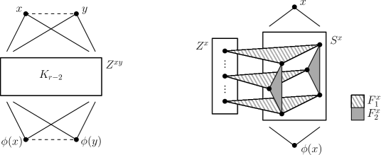
Figure 1. Left: Subgraph of $T_{1}$ associated with $xy\in E(H)$. Right: Subgraph of $T_{2}$ associated with $x\in V(H)$ in the case when $r=4$.

Claim 1: If $T$ satisfies (a)–(n), then $T$ is an $(H,H^{\prime})_{r}$-transformer.

Proof of Claim 1. Note that $H\cup E_{H}\cup E_{Z}$ can be decomposed into $e(H)$ copies of $K_{r}$, where each copy of $K_{r}$ has vertex set $\{x,y\}\cup Z^{xy}$ for some edge $xy\in E(H)$. Similarly, $H^{\prime}\cup E_{H^{\prime}}\cup E_{Z}$ can be decomposed into $e(H)$ copies of $K_{r}$.

For each $x\in V(H)$, note that $(E_{H^{\prime}}\cup E_{S}^{\prime})[\{\phi(x)\},S^{x}\cup Z^{x}]\cup F^{x}_{1}$ and $E_{S}[\{x\},S^{x}]\cup F^{x}_{2}$ are edge-disjoint and have $K_{r}$-decompositions. Since

$$T_{2}\cup E_{H^{\prime}}=\bigcup_{x\in V(H)}\big{(}(E_{H^{\prime}}\cup E_{S}^{\prime})[\{\phi(x)\},S^{x}\cup Z^{x}]\cup F^{x}_{1}\big{)}\cup\bigcup_{x\in V(H)}\big{(}E_{S}[\{x\},S^{x}]\cup F^{x}_{2}\big{)},$$

it follows that $T_{2}\cup E_{H^{\prime}}$ has a $K_{r}$-decomposition. Similarly, for each $x\in V(H)$, $(E_{H}\cup E_{S})[\{x\},S^{x}\cup Z^{x}]\cup F^{x}_{1}$ and $E_{S}^{\prime}[\{\phi(x)\},S^{x}]\cup F^{x}_{2}$ are edge-disjoint and have $K_{r}$-decompositions, so $T_{2}\cup E_{H}$ has a $K_{r}$-decomposition.

To summarise, $H\cup E_{H}\cup E_{Z}$, $H^{\prime}\cup E_{H^{\prime}}\cup E_{Z}$, $T_{2}\cup E_{H}$ and $T_{2}\cup E_{H^{\prime}}$ all have $K_{r}$-decompositions. Therefore, $T\cup H=(H\cup E_{H}\cup E_{Z})\cup(T_{2}\cup E_{H^{\prime}})$ has a $K_{r}$-decomposition, as does $T\cup H^{\prime}=(H^{\prime}\cup E_{H^{\prime}}\cup E_{Z})\cup(T_{2}\cup E_{H})$. Hence $T$ is an $(H,H^{\prime})_{r}$-transformer.

Claim 2: $G$ contains a graph $T$ satisfying (a)–(n) such that $V(T)\cap B\subseteq V(H\cup H^{\prime})$.

Proof of Claim 2. We begin by finding a copy of $T_{1}$ in $G$. It will be useful to note that, for any graph $T$ which satisfies (a)–(n), $T_{1}$ is $r$-partite with vertex classes $(V(H\cup H^{\prime})\cap V_{j})\cup\{z^{xy}_{j}:xy\in E(H)\text{ and }x,y\notin V_{j}\}$ where $1\leq j\leq r$. Also, $T[V(H\cup H^{\prime})]$ is empty and every vertex $z\in V(T_{1})\setminus V(H\cup H^{\prime})$ satisfies

(6.1) $$d_{T_{1}}(z)=2+(r-3)+2=r+1.$$

So $T_{1}$ has degeneracy $r+1$ rooted at $V(H\cup H^{\prime})$. Since $\hat{\delta}(G)\geq(1-1/(r+1)+{\varepsilon}/2)n+|B|$, we can find a copy of $T_{1}$ in $G$ such that $V(T_{1})\cap B\subseteq V(H\cup H^{\prime})$.

We now show that, after fixing $T_{1}$, we can extend $T_{1}$ to $T$ by finding a copy of $T_{2}$. Consider any ordering $x_{1},\dots,x_{|H|}$ on the vertices of $H$. Suppose we have already chosen $S^{x_{1}},\dots,S^{x_{q-1}}$, $F^{x_{1}}_{1},\dots,F^{x_{q-1}}_{1}$ and $F^{x_{1}}_{2},\dots,F^{x_{q-1}}_{2}$ and we are currently embedding $S^{x_{q}}$. Let $B^{\prime}:=B\cup V(T_{1})\cup\bigcup_{i=1}^{q-1}S^{x_{i}}$; that is, $B^{\prime}$ is the set of vertices that are unavailable for $S^{x_{q}}$, either because they have been used previously or they lie $B$. Note that $|B^{\prime}|\leq|T|+|B|\leq 2\eta n$. We will choose suitable vertices for $S^{x_{q}}$ in the common neighbourhood of $x_{q}$ and $\phi(x_{q})$.

To simplify notation, we write $x:=x_{q}$ and assume that $x\in V_{1}$ (the argument is identical in the other cases). Choose a set $V^{\prime}\subseteq(N_{G}(x)\cap N_{G}(\phi(x)))\setminus B^{\prime}$ which is maximal subject to $|V_{2}^{\prime}|=\dots=|V_{r}^{\prime}|$ (recall that $V_{j}^{\prime}=V^{\prime}\cap V_{j}$). Note that for each $2\leq j\leq r$, we have

$$|V_{j}^{\prime}|\geq(1-1/(r+1)+{\varepsilon})n-(1/(r+1)-{\varepsilon})n-|B^{\prime}|\geq(1-2/(r+1))n.$$

Let $n^{\prime}:=|V_{2}^{\prime}|$. For every $2\leq j\leq r$ and every $v\in V(G)\setminus V_{j}$, we have

(6.2) $$d_{G}(v,V_{j}^{\prime})\geq n^{\prime}-(1/(r+1)-{\varepsilon})n\geq(1-1/(r-1)+{\varepsilon})n^{\prime}.$$

Roughly speaking, we will choose $S^{x}$ as a random subset of $V^{\prime}$. For each $2\leq j\leq r$, choose each vertex of $V_{j}^{\prime}$ independently with probability $p:=(1+{\varepsilon}/8)s/n^{\prime}$ and let $S_{j}^{\prime}$ be the set of chosen vertices. Note that, for each $j$, $\mathbb{E}(|S_{j}^{\prime}|)=n^{\prime}p=(1+{\varepsilon}/8)s$. We can apply Lemma 2.2 to see that

$$\mathbb{P}(||S_{j}^{\prime}|-(1+{\varepsilon}/8)s|\geq{\varepsilon}s/8) \leq\mathbb{P}(||S_{j}^{\prime}|-(1+{\varepsilon}/8)s|\geq{\varepsilon}\mathbb{E}(|S_{j}^{\prime}|)/10)$$

(6.3) $$\leq 2e^{-{\varepsilon}^{2}s/300}\leq 1/4(r-1).$$

Given a vertex $v\in V(G)$ and $2\leq j\leq r$ such that $v\notin V_{j}$, note that

$$\mathbb{E}(d_{G}(v,S^{\prime}_{j}))\stackrel{{\scriptstyle(\ref{eq:V'deg})}}{{\geq}}(1-1/(r-1)+{\varepsilon})n^{\prime}p>(1-1/(r-1)+{\varepsilon})s.$$

We will say that a vertex $v\in V(G)$ is bad if there exists $2\leq j\leq r$ such that $v\notin V_{j}$ and $d_{G}(v,S^{\prime}_{j})<(1-1/(r-1)+3{\varepsilon}/4)s$, that is, the degree of $v$ in $S^{\prime}_{j}$ is lower than expected. We can again apply Lemma 2.2 to see that

$$\mathbb{P}(d_{G}(v,S^{\prime}_{j})\leq(1-1/(r-1)+3{\varepsilon}/4)s) \leq\mathbb{P}(|d_{G}(v,S^{\prime}_{j})-\mathbb{E}(d_{G}(v,S^{\prime}_{j}))|\geq{\varepsilon}s/4)$$

$$\leq\mathbb{P}(|d_{G}(v,S^{\prime}_{j})-\mathbb{E}(d_{G}(v,S^{\prime}_{j}))|\geq{\varepsilon}\mathbb{E}(d_{G}(v,S^{\prime}_{j}))/10)$$

$$\leq 2e^{-{\varepsilon}^{2}s/600}.$$

So $\mathbb{P}(v\text{ is bad})\leq 2(r-1)e^{-{\varepsilon}^{2}s/600}\leq e^{-s^{1/2}}$. Let $S^{\prime}:=\bigcup_{j=2}^{r}S^{\prime}_{j}$. We say that the set $S^{\prime}$ is bad if $S^{\prime}\cup Z^{x}$ contains a bad vertex. We have

$$\mathbb{P}(S^{\prime}\text{ is bad}) \leq\sum_{v\in V^{\prime}}\mathbb{P}(v\in S^{\prime}\text{ and }v\text{ is bad})+\sum_{v\in Z^{x}}\mathbb{P}(v\text{ is bad})$$

$$=\sum_{v\in V^{\prime}}\mathbb{P}(v\in S^{\prime})\mathbb{P}(v\text{ is bad})+\sum_{v\in Z^{x}}\mathbb{P}(v\text{ is bad})$$

(6.4) $$\leq(n^{\prime}p+(b-1)(r-2))e^{-s^{1/2}}\leq 2se^{-s^{1/2}}\leq 1/4.$$

We apply (6.3) and (6.4) to see that with probability at least $1/2$, the set $S^{\prime}$ chosen in this way is not bad and, for each $2\leq j\leq r$, we have $s\leq|S_{j}^{\prime}|\leq(1+{\varepsilon}/4)s$. Choose one such set $S^{\prime}$. Delete at most ${\varepsilon}s/4$ vertices from each $S_{j}^{\prime}$ to obtain sets $S^{x}_{j}$ satisfying $|S^{x}_{2}|=\dots=|S^{x}_{r}|=s$. Let $S^{x}:=\bigcup_{j=2}^{r}S^{x}_{j}$. Since $S^{\prime}$ was not bad, for each $2\leq j\leq r$ and each vertex $v\in(S^{x}\cup Z^{x})\setminus V_{j}$,

(6.5) $$d_{G}(v,S^{x}_{j})\geq(1-1/(r-1)+3{\varepsilon}/4)s-{\varepsilon}s/4=(1-1/(r-1)+{\varepsilon}/2)s.$$

We now show that we can find $F^{x}_{1}$ and $F^{x}_{2}$ satisfying (j)–(m). Let $G^{x}:=G[Z^{x}\cup S^{x}]-G[Z^{x}]$. Note that $G^{x}$ is a balanced $(r-1)$-partite graph with vertex classes of size $n_{x}$ where $s\leq n_{x}\leq s+(r-2)(b-1)/(r-1)<s+b$. Using (6.5), we see that

$$\hat{\delta}(G^{x})\geq(1-1/(r-1)+{\varepsilon}/2)s\geq(1-1/(r-1)+{\varepsilon}/3)n_{x}.$$

So, using Theorem 6.2, we can find a perfect $K_{r-1}$-matching $F^{x}_{1}$ in $G^{x}$. Finally, let $G^{\prime}:=G-F^{x}_{1}$ and use (6.5) to see that

$$\hat{\delta}(G^{\prime}[S^{x}])\geq(1-1/(r-1)+{\varepsilon}/3)s.$$

So we can again apply Theorem 6.2, to find a perfect $K_{r-1}$-matching $F^{x}_{2}$ in $G^{\prime}[S^{x}]$. In this way, we find a copy of $T$ satisfying (a)–(n) such that $V(T)\cap B\subseteq V(H\cup H^{\prime})$.

This completes the proof of Lemma 6.1.        $\square$

We now construct our absorber by combining several suitable transformers.

Let $H$ be an $r$-partite multigraph on $(\tilde{V}_{1},\dots,\tilde{V}_{r})$ with $\tilde{V}_{i}\subset V_{i}$ for each $1\leq i\leq r$, and let $xy\in E(H)$. A $K_{r}$-expansion of $xy$ is defined as follows. Consider a copy $F_{xy}$ of $K_{r}$ on vertex set $\{u_{1},\dots,u_{r}\}$ such that $u_{j}\in V_{j}\setminus V(H)$ for all $1\leq j\leq r$. Let $j_{1},j_{2}$ be such that $x\in V_{j_{1}}$ and $y\in V_{j_{2}}$. Delete $xy$ from $H$ and $u_{j_{1}}u_{j_{2}}$ from $F_{xy}$ and add edges joining $x$ to $u_{j_{2}}$ and joining $y$ to $u_{j_{1}}$. Let $H_{\text{exp}}$ be the graph obtained by $K_{r}$-expanding every edge of $H$, where the $F_{xy}$ are chosen to be vertex-disjoint for different edges $xy\in E(H)$.

Fact 6.3.

Suppose that the graph $H^{\prime}$ is obtained from a graph $H$ by $K_{r}$-expanding the edge $xy\in E(H)$ as above. Then the graph obtained from $H^{\prime}$ by identifying $x$ and $u_{j_{1}}$ is $H$ with a copy of $K_{r}$ attached to $x$.

Let $h\in\mathbb{N}$. We define a graph $M_{h}$ as follows. Take a copy of $K_{r}$ on $V$ (consisting of one vertex in each $V_{j}$) and replace each edge by $h$ multiedges. Let $M$ denote the resulting multigraph. Let $M_{h}:=M_{\text{exp}}$ be the graph obtained by $K_{r}$-expanding every edge of $M$. We have $|M_{h}|=r+hr\binom{r}{2}$. Note that $M_{h}$ has degeneracy $r-1$. To see this, list all vertices in $V(M)$ (in any order) followed by the vertices in $V(M_{h}\setminus M)$ (in any order).

We will now apply Lemma 6.1 twice in order to find an $(H,M_{h})_{r}$-transformer in $G$.

Lemma 6.4.

Let $r\geq 3$ and $1/n\ll\eta\ll 1/s\ll{\varepsilon},1/b,1/r\leq 1$. Let $G$ be an $r$-partite graph on $V=(V_{1},\dots,V_{r})$ with $|V_{1}|=\dots=|V_{r}|=n$. Suppose that $\hat{\delta}(G)\geq(1-1/(r+1)+{\varepsilon})n$. Let $H$ be a $K_{r}$-divisible graph on $V$ with $|H|\leq b$. Let $h:=e(H)/\binom{r}{2}$. Let $M^{\prime}_{h}$ be a partition-respecting copy of $M_{h}$ on $V$ which is vertex-disjoint from $H$. Let $B\subseteq V$ be a set of at most $\eta n$ vertices. Then $G$ contains an $(H,M^{\prime}_{h})_{r}$-transformer $T$ such that $V(T)\cap B\subseteq V(H\cup M^{\prime}_{h})$ and $|T|\leq 3s^{2}$.

Proof. We construct a graph $H_{\text{att}}$ as follows. Start with the graph $H$. For each edge of $H$, arbitrarily choose one of it endpoints $x$ and attach a copy of $K_{r}$ (found in $G\setminus((V(H\cup M^{\prime}_{h})\cup B)\setminus\{x\})$) to $x$. The copies of $K_{r}$ should be chosen to be vertex-disjoint outside $V(H)$. Write $H_{\text{att}}$ for the resulting graph. Let $H_{\text{exp}}^{\prime}$ be a partition-respecting copy of $H_{\text{exp}}$ in $G\setminus(V(H_{\text{att}}\cup M^{\prime}_{h})\cup B)$. Note that we are able to find these graphs since both have degeneracy $r-1$ and $\hat{\delta}(G)\geq(1-1/(r+1)+{\varepsilon})n$.

By Fact 6.3, $H_{\text{att}}$ is a partition-respecting copy of a graph obtained from $H_{\text{exp}}^{\prime}$ by identifying vertices, and this is also the case for $M^{\prime}_{h}$. To see the latter, for each $1\leq j\leq r$, identify all vertices of $H_{\text{exp}}^{\prime}$ lying in $V_{j}$. (We are able to do this since these vertices are non-adjacent with disjoint neighbourhoods.)

Apply Lemma 6.1 to find an $(H_{\text{exp}}^{\prime},H_{\text{att}})_{r}$-transformer $T^{\prime}$ in $G-M^{\prime}_{h}$ such that $V(T^{\prime})\cap B\subseteq V(H)$ and $|T^{\prime}|\leq s^{2}$. Then apply Lemma 6.1 again to find an $(H_{\text{exp}}^{\prime},M^{\prime}_{h})_{r}$-transformer $T^{\prime\prime}$ in $G-(H_{\text{att}}\cup T^{\prime})$ such that $V(T^{\prime\prime})\cap B\subseteq V(M^{\prime}_{h})$ and $|T^{\prime\prime}|\leq s^{2}$.

Let $T:=T^{\prime}\cup T^{\prime\prime}\cup H_{\text{exp}}^{\prime}\cup(H_{\text{att}}-H)$. Then $T$ is edge-disjoint from $H\cup M^{\prime}_{h}$. Note that

$$T\cup H=(T^{\prime}\cup H_{\text{att}})\cup(T^{\prime\prime}\cup H_{\text{exp}}^{\prime})\hskip 6.0pt\text{ and}$$

$$T\cup M^{\prime}_{h}=(T^{\prime}\cup H_{\text{exp}}^{\prime})\cup(T^{\prime\prime}\cup M^{\prime}_{h})\cup(H_{\text{att}}-H),$$

both of which have $K_{r}$-decompositions. Therefore $T$ is an $(H,M^{\prime}_{h})_{r}$-transformer. Moreover, $|T|\leq 3s^{2}$. Finally, observe that $V(T)\cap B=V(T^{\prime}\cup T^{\prime\prime}\cup H_{\text{att}})\cap B\subseteq V(H\cup M^{\prime}_{h})$.        $\square$

We now have all of the necessary tools to find an absorber for $H$ in $G$.

Lemma 6.5.

Let $r\geq 3$ and let $1/n\ll\eta\ll 1/s\ll{\varepsilon},1/b,1/r\leq 1$. Let $G$ be an $r$-partite graph on $V=(V_{1},\dots,V_{r})$ with $|V_{1}|=\dots=|V_{r}|=n$. Suppose that $\hat{\delta}(G)\geq(1-1/(r+1)+{\varepsilon})n$. Let $H$ be a $K_{r}$-divisible graph on $V$ with $|H|\leq b$. Let $B\subseteq V$ be a set of at most $\eta n$ vertices. Then $G$ contains an absorber $A$ for $H$ such that $V(A)\cap B\subseteq V(H)$ and $|A|\leq s^{3}$.

Proof. Let $h:=e(H)/\binom{r}{2}$. Let $G^{\prime}:=G\setminus(V(H)\cup B)$. Write $hK_{r}$ for the graph consisting of $h$ vertex-disjoint copies of $K_{r}$. Since $\hat{\delta}(G^{\prime})\geq(1-1/(r+1)+{\varepsilon}/2)n$, we can choose vertex-disjoint (partition-respecting) copies of $M_{h}$ and $hK_{r}$ in $G^{\prime}$ (and call these $M_{h}$ and $hK_{r}$ again). Use Lemma 6.4 to find an $(H,M_{h})_{r}$-transformer $T^{\prime}$ in $G-hK_{r}$ such that $V(T^{\prime})\cap B\subseteq V(H)$ and $|T^{\prime}|\leq 3s^{2}$. Apply Lemma 6.4 again to find an $(hK_{r},M_{h})_{r}$-transformer $T^{\prime\prime}$ in $G-(H\cup T^{\prime})$ which avoids $B$ and satisfies $|T^{\prime\prime}|\leq 3s^{2}$. It is easy to see that $T:=T^{\prime}\cup T^{\prime\prime}\cup M_{h}$ is an $(H,hK_{r})_{r}$-transformer.

Let $A:=T\cup hK_{r}$. Note that both $A$ and $A\cup H=(T\cup H)\cup hK_{r}$ have $K_{r}$-decompositions. So $A$ is an absorber for $H$. Moreover, $V(A)\cap B\subseteq V(T^{\prime})\cap B\subseteq V(H)$ and $|A|\leq s^{3}$.        $\square$

6.1. Absorbing sets

Let $\mathcal{H}$ be a collection of graphs on the vertex set $V=(V_{1},\dots,V_{r})$. We say that $\mathcal{A}$ is an absorbing set for $\mathcal{H}$ if $\mathcal{A}$ is a collection of edge-disjoint graphs and, for every $H\in\mathcal{H}$ and every $K_{r}$-divisible subgraph $H^{\prime}\subseteq H$, there is a distinct $A_{H^{\prime}}\in\mathcal{A}$ such that $A_{H^{\prime}}$ is an absorber for $H^{\prime}$.

Lemma 6.6.

Let $r\geq 3$ and $1/n\ll\eta\ll{\varepsilon},1/b,1/r\leq 1$. Let $G$ be an $r$-partite graph on $V=(V_{1},\dots,V_{r})$ with $|V_{1}|=\dots=|V_{r}|=n$. Suppose that $\hat{\delta}(G)\geq(1-1/(r+1)+{\varepsilon})n$. Let $m\leq\eta n^{2}$ and let $\mathcal{H}$ be a collection of $m$ edge-disjoint graphs on $V=(V_{1},\dots,V_{r})$ such that each vertex $v\in V$ appears in at most $\eta n$ of the elements of $\mathcal{H}$ and $|H|\leq b$ for each $H\in\mathcal{H}$. Then $G$ contains an absorbing set $\mathcal{A}$ for $\mathcal{H}$ such that $\Delta(\bigcup\mathcal{A})\leq{\varepsilon}n$.

We repeatedly use Lemma 6.5 and aim to avoid any vertices which have been used too often.

Proof. Enumerate the $K_{r}$-divisible subgraphs of all $H\in\mathcal{H}$ as $H_{1},\dots,H_{m^{\prime}}$. Note that each $H\in\mathcal{H}$ can have at most $2^{e(H)}\leq 2^{\binom{b}{2}}$ $K_{r}$-divisible subgraphs so $m^{\prime}\leq 2^{\binom{b}{2}}\eta n^{2}$. For each $v\in V(G)$ and each $0\leq j\leq m^{\prime}$, let $s(v,j)$ be the number of indices $1\leq i\leq j$ such that $v\in V(H_{i})$. Note that $s(v,j)\leq 2^{\binom{b}{2}}\eta n$.

Let $s\in\mathbb{N}$ be such that $\eta\ll 1/s\ll{\varepsilon},1/b,1/r$. Suppose that we have already found absorbers $A_{1},\dots,A_{j-1}$ for $H_{1},\dots,H_{j-1}$ respectively such that $|A_{i}|\leq s^{3}$, for all $1\leq i\leq j-1$, and, for every $v\in V(G)$,

(6.6) $$d_{G_{j-1}}(v)\leq\eta^{1/2}n+(s(v,j-1)+1)s^{3},$$

where $G_{j-1}:=\bigcup_{1\leq i\leq j-1}A_{i}$. We show that we can find an absorber $A_{j}$ for $H_{j}$ in $G-G_{j-1}$ which satisfies (6.6) with $j$ replacing $j-1$.

Let $B:=\{v\in V(G):d_{G_{j-1}}(v)\geq\eta^{1/2}n\}$. We have

$$|B|\leq\frac{2e(G_{j-1})}{\eta^{1/2}n}\leq\frac{2m^{\prime}\binom{s^{3}}{2}}{\eta^{1/2}n}\leq\frac{2^{\binom{b}{2}+1}\eta n^{2}s^{6}}{\eta^{1/2}n}\leq\eta^{1/3}n.$$

We have

$$\hat{\delta}(G-G_{j-1}) \stackrel{{\scriptstyle\mathclap{\eqref{eq:emb1'}}}}{{\geq}}(1-1/(r+1)+{\varepsilon})n-\eta^{1/2}n-(s(v,j-1)+1)s^{3}$$

$$\geq(1-1/(r+1)+{\varepsilon})n-\eta^{1/2}n-(2^{\binom{b}{2}}\eta n+1)s^{3}>(1-1/(r+1)+{\varepsilon}/2)n.$$

So we can apply Lemma 6.5 (with ${\varepsilon}/2$, $\eta^{1/3}$, $G-G_{j-1}$ and $H_{j}$ playing the roles of ${\varepsilon}$, $\eta$, $G$ and $H$) to find an absorber $A_{j}$ for $H_{j}$ in $G-G_{j-1}$ such that $V(A_{j})\cap B\subseteq V(H_{j})$ and $|A_{j}|\leq s^{3}$.

We now check that (6.6) holds with $j$ replacing $j-1$. If $v\in V(G)\setminus B$, this is clear. Suppose then that $v\in B$. If $v\in V(A_{j})$, then $v\in V(H_{j})$ and $s(v,j)=s(v,j-1)+1$. So in all cases,

$$d_{G_{j}}(v)\leq\eta^{1/2}n+(s(v,j)+1)s^{3},$$

as required.

Continue in this way until we have found an absorber $A_{i}$ for each $H_{i}$. Then $\mathcal{A}:=\{A_{i}:1\leq i\leq m^{\prime}\}$ is an absorbing set. Using (6.6),

$$\Delta\big{(}\bigcup\mathcal{A}\big{)}=\Delta(G_{m^{\prime}})\leq\eta^{1/2}n+(2^{\binom{b}{2}}\eta n+1)s^{3}\leq{\varepsilon}n,$$

as required.        $\square$

7. Partitions and random subgraphs

In this section we consider a sequence $\mathcal{P}_{1},\dots,\mathcal{P}_{\ell}$ of successively finer partitions which will underlie our iterative absorption process. We will also construct corresponding sparse quasirandom subgraphs $R_{i}$ which will be used to ‘smooth out’ the leftover from the approximate decomposition in each step of the process.

Recall from Section 2 that a $k$-partition is a partition satisfying (Pa1) and (Pa2). Let $G$ be an $r$-partite graph on $(V_{1},\dots,V_{r})$. An $(\alpha,k,\delta)$-partition for $G$ on $(V_{1},\dots,V_{r})$ is a $k$-partition $\mathcal{P}=\{U^{1},\dots,U^{k}\}$ of $V(G)$ such that in the following hold:

1. for each $v\in V(G)$, each $1\leq i\leq k$ and each $1\leq j\leq r$,

   $$|d_{G}(v,U^{i}_{j})-d_{G}(v,V_{j})/k|<\alpha|U^{i}_{j}|;$$

2. for each $1\leq i\leq k$, each $1\leq j\leq r$ and each $v\notin V_{j}$, $d_{G}(v,U^{i}_{j})\geq\delta|U^{i}_{j}|$.

The following proposition guarantees a $(n^{-1/3}/2,k,\delta-n^{-1/3}/2)$-partition of any sufficiently large balanced $r$-partite graph $G$ with $\hat{\delta}(G)\geq\delta n$. To prove this result, it suffices to consider an equitable partition $U^{1}_{j},U^{2}_{j},\dots,U^{k}_{j}$ of $V_{j}$ chosen uniformly at random (with $|U^{1}_{j}|\leq\dots\leq|U^{k}_{j}|$).

Proposition 7.1.

Let $k,r\in\mathbb{N}$. There exists $n_{0}$ such that if $n\geq n_{0}$ and $G$ is any $r$-partite graph on $(V_{1},\dots,V_{r})$ with $|V_{1}|=\dots=|V_{r}|=n$ and $\hat{\delta}(G)\geq\delta n$, then $G$ has a $(\nu,k,\delta-\nu)$-partition, where $\nu:=n^{-1/3}/2$.∎

We say that $\mathcal{P}_{1},\mathcal{P}_{2},\dots,\mathcal{P}_{\ell}$ is an $(\alpha,k,\delta,m)$-partition sequence for $G$ on $(V_{1},\dots,V_{r})$ if, writing $\mathcal{P}_{0}:=\{V(G)\}$,

1. for each $1\leq i\leq\ell$, $\mathcal{P}_{i}$ refines $\mathcal{P}_{i-1}$;

2. for each $1\leq i\leq\ell$ and each $W\in\mathcal{P}_{i-1}$, $\mathcal{P}_{i}[W]$ is an $(\alpha,k,\delta)$-partition for $G[W]$;

3. for each $1\leq i\leq\ell$, all $1\leq j_{1},j_{2},j_{3}\leq r$ with $j_{1}\neq j_{2},j_{3}$, each $W\in\mathcal{P}_{i-1}$, each $U\in\mathcal{P}_{i}[W]$ and each $v\in W_{j_{1}}$,

   $$|d_{G}(v,U_{j_{2}})-d_{G}(v,U_{j_{3}})|<\alpha|U_{j_{1}}|;$$

4. for each $U\in\mathcal{P}_{\ell}$ and each $1\leq j\leq r$, $|U_{j}|=m$ or $m-1$.

Note that (S2) and (Pa2) together imply that $|U_{j_{1}}|=|U_{j_{2}}|$ for each $1\leq i\leq\ell$, each $U\in\mathcal{P}_{i}$ and all $1\leq j_{1},j_{2}\leq r$.

By successive applications of Proposition 7.1, we immediately obtain the following result which guarantees the existence of a suitable partition sequence (for details see [27]).

Lemma 7.2.

Let $k,r\in\mathbb{N}$ with $k\geq 2$ and let $0<\alpha<1$. There exists $m_{0}$ such that, for all $m^{\prime}\geq m_{0}$, any $K_{r}$-divisible graph $G$ on $(V_{1},\dots,V_{r})$ with $|V_{1}|=\dots=|V_{r}|=n\geq km^{\prime}$ and $\hat{\delta}(G)\geq\delta n$ has an $(\alpha,k,\delta-\alpha,m)$-partition sequence for some $m^{\prime}\leq m\leq km^{\prime}$. ∎

Suppose that we are given a $k$-partition $\mathcal{P}$ of $G$. The following proposition finds a quasirandom spanning subgraph $R$ of $G$ so that each vertex in $R$ has roughly the expected number of neighbours in each set $U\in\mathcal{P}$. The proof is an easy application of Lemma 2.1.

Proposition 7.3.

Let $1/n\ll\alpha,\rho,1/k,1/r\leq 1$. Let $G$ be an $r$-partite graph on $(V_{1},\dots,V_{r})$ with $|V_{1}|=\dots=|V_{r}|=n$. Suppose that $\mathcal{P}$ is a $k$-partition for $G$. Let $\mathcal{S}$ be a collection of at most $n^{2}$ subsets of $V(G)$. Then there exists $R\subseteq G[\mathcal{P}]$ such that for all $1\leq j\leq r$, all distinct $x,y\in V(G)$, all $U\in\mathcal{P}$ and all $S\in\mathcal{S}$:

• $|d_{R}(x,U_{j})-\rho d_{G[\mathcal{P}]}(x,U_{j})|<\alpha|U_{j}|$;

• $|d_{R}(\{x,y\},U_{j})-\rho^{2}d_{G[\mathcal{P}]}(\{x,y\},U_{j})|<\alpha|U_{j}|$;

• $|d_{G}(y,N_{R}(x,U_{j}))-\rho d_{G}(y,N_{G[\mathcal{P}]}(x,U_{j}))|<\alpha|U_{j}|$;

• $|d_{R}(y,S_{j})-\rho d_{G[\mathcal{P}]}(y,S_{j})|<\alpha n$. ∎

We need to reserve some quasirandom subgraphs $R_{i}$ of $G$ at the start of our proof, whilst the graph $G$ is still almost balanced with respect to the partition sequence. We will add the edges of $R_{i}$ back after finding an approximate decomposition of $G[\mathcal{P}_{i}]$ in order to assume the leftover from this approximate decomposition is quasirandom. The next lemma gives us suitable subgraphs for $R_{i}$.

Lemma 7.4.

Let $1/m\ll\alpha\ll\rho,1/k,1/r\leq 1$. Let $G$ be an $r$-partite graph on $(V_{1},\dots,V_{r})$ with $|V_{1}|=\dots=|V_{r}|$. Suppose that $\mathcal{P}_{1},\dots,\mathcal{P}_{\ell}$ is a $(1,k,0,m)$-partition sequence for $G$. Let $\mathcal{P}_{0}:=\{V(G)\}$ and, for each $0\leq q\leq\ell$, let $G_{q}:=G[\mathcal{P}_{q}]$. Then there exists a sequence of graphs $R_{1},\dots,R_{\ell}$ such that $R_{q}\subseteq G_{q}-G_{q-1}$ for each $q$ and the following holds. For all $1\leq q\leq\ell$, all $1\leq j\leq r$, all $W\in\mathcal{P}_{q-1}$, all distinct $x,y\in W$ and all $U\in\mathcal{P}_{q}[W]$:

1. $|d_{R_{q}}(x,U_{j})-\rho d_{G_{q}}(x,U_{j})|<\alpha|U_{j}|$;

2. $|d_{R_{q}}(\{x,y\},U_{j})-\rho^{2}d_{G_{q}}(\{x,y\},U_{j})|<\alpha|U_{j}|$;

3. $d_{G_{q+1}^{\prime}}(y,N_{R_{q}}(x,U_{j}))\geq\rho d_{G_{q+1}}(y,N_{G_{q}}(x,U_{j}))-3\rho^{2}|U_{j}|$, where $G_{q+1}^{\prime}:=G_{q+1}-R_{q+1}$ if $q\leq\ell-1$, $G_{\ell+1}^{\prime}:=G$ and $G_{\ell+1}:=G$.

Proof. For $1\leq q\leq\ell$, we say that the sequence of graphs $R_{1},\ldots,R_{q}$ is good if $R_{i}\subseteq G_{i}-G_{i-1}$ and for all $1\leq i\leq q$, all $1\leq j\leq r$, all $W\in\mathcal{P}_{i-1}$, all distinct $x,y\in W$ and all $U\in\mathcal{P}_{i}[W]$:

1. (i) and (ii) hold (with $q$ replaced by $i$);

2. $|d_{G_{i+1}}(y,N_{R_{i}}(x,U_{j}))-\rho d_{G_{i+1}}(y,N_{G_{i}}(x,U_{j}))|<\alpha|U_{j}|$;

3. if $i\leq q-1$, $d_{R_{i+1}}(y,N_{R_{i}}(x,U_{j}))<\rho d_{G_{i+1}}(y,N_{R_{i}}(x,U_{j}))+\alpha|U_{j}|$.

Suppose $1\leq q\leq\ell$ and we have found a good sequence of graphs $R_{1},\ldots,R_{q-1}$. We will find $R_{q}$ such that $R_{1},\dots,R_{q}$ is good. Let $W\in\mathcal{P}_{q-1}$, let $\mathcal{S}_{1}$ be the empty set and, if $q\geq 2$, let $W^{\prime}\in\mathcal{P}_{q-2}$ be such that $W\subseteq W^{\prime}$ and let $\mathcal{S}_{q}:=\{N_{R_{q-1}}(x,W):x\in W^{\prime}\}$. Apply Proposition 7.3 (with $|W|/r$, $G_{q+1}[W]$, $\mathcal{P}_{q}[W]$ and $\mathcal{S}_{q}$ playing the roles of $n$, $G$, $\mathcal{P}$ and $\mathcal{S}$) to find $R_{W}\subseteq G_{q+1}[W][\mathcal{P}_{q}[W]]=G_{q}[W]$ such that:

$$|d_{R_{W}}(x,U_{j})-\rho d_{G_{q}}(x,U_{j})|<\alpha|U_{j}|,$$

$$|d_{R_{W}}(\{x,y\},U_{j})-\rho^{2}d_{G_{q}}(\{x,y\},U_{j})|<\alpha|U_{j}|,$$

$$|d_{G_{q+1}}(y,N_{R_{W}}(x,U_{j}))-\rho d_{G_{q+1}}(y,N_{G_{q}}(x,U_{j}))|<\alpha|U_{j}|,$$

(7.1) $$|d_{R_{W}}(y,S_{j})-\rho d_{G_{q}}(y,S_{j})|<\alpha|W_{j}|,$$

for all $1\leq j\leq r$, all distinct $x,y\in W$, all $U\in\mathcal{P}_{q}[W]$ and all $S\in\mathcal{S}_{q}$. Set $R_{q}:=\bigcup_{W\in\mathcal{P}_{q-1}}R_{W}$. It is clear that $R_{1},\dots,R_{q}$ satisfy (a) and (b). We now check that (c) holds when $1\leq i=q-1$. Let $1\leq j\leq r$, $W\in\mathcal{P}_{q-2}$, $x,y\in W$ be distinct and $U\in\mathcal{P}_{q-1}[W]$. If $y\notin U$, then $d_{R_{q}}(y,U_{j})=0$ and so (c) holds. If $y\in U$, then $d_{R_{q}}(y,N_{R_{q-1}}(x,U))=d_{R_{U}}(y,N_{R_{q-1}}(x,U))$ and (c) follows by replacing $W$ and $S$ by $U$ and $N_{R_{q-1}}(x,U)$ in property (7.1). So $R_{1},\dots,R_{q}$ is good.

So $G$ contains a good sequence of graphs $R_{1},\dots,R_{\ell}$. We will now check that this sequence also satisfies (iii). If $q=\ell$, this follows immediately from (b). Let $1\leq q<\ell$, $1\leq j\leq r$, $W\in\mathcal{P}_{q-1}$, $x,y\in W$ be distinct and $U\in\mathcal{P}_{q}[W]$. We have

$$d_{R_{q+1}}(y,N_{R_{q}}(x,U_{j})) \stackrel{{\scriptstyle\mathclap{\eqref{item:c}}}}{{<}}\rho d_{G_{q+1}}(y,N_{R_{q}}(x,U_{j}))+\alpha|U_{j}|$$

$$\stackrel{{\scriptstyle\mathclap{\eqref{item:b}}}}{{<}}\rho^{2}d_{G_{q+1}}(y,N_{G_{q}}(x,U_{j}))+(\alpha\rho+\alpha)|U_{j}|\leq 2\rho^{2}|U_{j}|.$$

Therefore,

$$d_{G_{q+1}^{\prime}}(y,N_{R_{q}}(x,U_{j})) =d_{G_{q+1}}(y,N_{R_{q}}(x,U_{j}))-d_{R_{q+1}}(y,N_{R_{q}}(x,U_{j}))$$

$$\stackrel{{\scriptstyle\mathclap{\eqref{item:b}}}}{{\geq}}\rho d_{G_{q+1}}(y,N_{G_{q}}(x,U_{j}))-3\rho^{2}|U_{j}|.$$

So $R_{1},\dots,R_{\ell}$ satisfy (i)–(iii).        $\square$

We apply Lemma 7.4 when $\mathcal{P}_{1},\dots,\mathcal{P}_{\ell}$ is an $(\alpha,k,1-1/r+{\varepsilon},m)$-partition sequence for $G$ to obtain the following result. For details of the proof, see [27].

Corollary 7.5.

Let $1/m\ll\alpha\ll\rho,1/k\ll{\varepsilon},1/r\leq 1$. Let $G$ be a $K_{r}$-divisible graph on $(V_{1},\dots,V_{r})$ with $|V_{1}|=\dots=|V_{r}|$. Suppose that $\mathcal{P}_{1},\dots,\mathcal{P}_{\ell}$ is an $(\alpha,k,1-1/r+{\varepsilon},m)$-partition sequence for $G$. Let $\mathcal{P}_{0}:=\{V(G)\}$ and $G_{q}:=G[\mathcal{P}_{q}]$ for $0\leq q\leq\ell$. There exists a sequence of graphs $R_{1},\dots,R_{\ell}$ such that $R_{q}\subseteq G_{q}-G_{q-1}$ for each $1\leq q\leq\ell$ and the following holds. For all $1\leq q\leq\ell$, all $1\leq j,j^{\prime}\leq r$, all $W\in\mathcal{P}_{q-1}$, all distinct $x,y\in W$ and all $U,U^{\prime}\in\mathcal{P}_{q}[W]$:

1. $d_{R_{q}}(x,U_{j})<\rho d_{G_{q}}(x,U_{j})+\alpha|U_{j}|$;

2. $d_{R_{q}}(\{x,y\},U_{j})<(\rho^{2}+\alpha)|U_{j}|$;

3. if $x\notin U\cup U^{\prime}\cup V_{j}\cup V_{j^{\prime}}$, $|d_{R_{q}}(x,U_{j})-d_{R_{q}}(x,U^{\prime}_{j^{\prime}})|<3\alpha|U_{j}|$;

4. if $x\notin U$, $y\in U$ and $x,y\notin V_{j}$, then

   $$d_{G_{q+1}^{\prime}}(y,N_{R_{q}}(x,U_{j}))\geq\rho(1-1/(r-1))d_{G_{q}}(x,U_{j})+\rho^{5/4}|U_{j}|,$$

   where $G_{q+1}^{\prime}:=G_{q+1}-R_{q+1}$ if $q\leq\ell-1$ and $G_{\ell+1}^{\prime}:=G$. ∎

8. A remainder of low maximum degree

The aim of this section is to prove the following lemma which lets us assume that the remainder of $G$ after finding an $\eta$-approximate decomposition has small maximum degree.

Lemma 8.1.

Let $1/n\ll\alpha\ll\eta\ll\gamma\ll{\varepsilon}<1/r<1$. Let $G$ be an $r$-partite graph on $(V_{1},\dots,V_{r})$ with $|V_{1}|=\dots=|V_{r}|=n$ and $\hat{\delta}(G)\geq(\hat{\delta}^{\eta}_{K_{r}}+{\varepsilon})n$. Suppose also that, for all $1\leq j_{1},j_{2}\leq r$ and every $v\notin V_{j_{1}}\cup V_{j_{2}}$,

(8.1) $$|d_{G}(v,V_{j_{1}})-d_{G}(v,V_{j_{2}})|<\alpha n.$$

Then there exists $H\subseteq G$ such that $G-H$ has a $K_{r}$-decomposition and $\Delta(H)\leq\gamma n$.

Our strategy for the proof of Lemma 8.1 is as follows. We first remove a sparse random subgraph $H_{1}$ from $G$. We will then remove a further graph $H_{2}$ of small maximum degree from $G-H_{1}$ to achieve that $G-(H_{1}\cup H_{2})$ is $K_{r}$-divisible. (The existence of such a graph $H_{2}$ is shown in Proposition 8.9.) The definition of $\delta^{\eta}_{K_{r}}$ then ensures that $G-(H_{1}\cup H_{2})$ has an $\eta$-approximate $K_{r}$-decomposition. We now consider the graph $R$ obtained from $G-H_{2}$ by deleting all edges in the copies of $K_{r}$ in this decomposition. Suppose that $v$ is a vertex whose degree in $R$ is too high. Our aim will be to find a $K_{r-1}$-matching in $H_{1}$ whose vertex set is the neighbourhood of $v$ in $G$. If $\rho$ denotes the edge-probability for the random subgraph $H_{1}$, then each vertex in $H_{1}$ is, on average, joined to at most $\rho d_{G}(v)/(r-1)\ll(1-1/(r-1)+{\varepsilon})d_{G}(v)/(r-1)$ vertices in each other part, so Theorem 6.2 alone is of no use. But Theorem 6.2 can be combined with the Regularity lemma in order to find the desired $K_{r-1}$-matching in $H_{1}$ (see Proposition 8.8).

8.1. Regularity

In this section, we introduce a version of the Regularity lemma which we will use to prove Lemma 8.1.

Let $G$ be a bipartite graph on $(A,B)$. For non-empty sets $X\subseteq A$, $Y\subseteq B$, we define the density of $G[X,Y]$ to be $d_{G}(X,Y):=e_{G}(X,Y)/|X||Y|$. Let ${\varepsilon}>0$. We say that $G$ is ${\varepsilon}$-regular if for all sets $X\subseteq A$ and $Y\subseteq B$ with $|X|\geq{\varepsilon}|A|$ and $|Y|\geq{\varepsilon}|B|$ we have

$$|d_{G}(A,B)-d_{G}(X,Y)|<{\varepsilon}.$$

The following simple result follows immediately from this definition.

Proposition 8.2.

Suppose that $0<\varepsilon\leq\alpha\leq 1/2$. Let $G$ be a bipartite graph on $(A,B)$. Suppose that $G$ is ${\varepsilon}$-regular with density $d$. If $A^{\prime}\subseteq A,B^{\prime}\subseteq B$ with $|A^{\prime}|\geq\alpha|A|$ and $|B^{\prime}|\geq\alpha|B|$ then $G[A^{\prime},B^{\prime}]$ is ${\varepsilon}/\alpha$-regular and has density greater than $d-\varepsilon$.∎

Proposition 8.2 shows that regularity is robust, that is, it is not destroyed by deleting even quite a large number of vertices. The next observation allows us to delete a small number of edges at each vertex and still maintain regularity. The proof again follows from the definition.

Proposition 8.3.

Let $n\in\mathbb{N}$ and let $0<\gamma\ll\varepsilon\leq 1$. Let $G$ be a bipartite graph on $(A,B)$ with $|A|=|B|=n$. Suppose that $G$ is ${\varepsilon}$-regular with density $d$. Let $H\subseteq G$ with $\Delta(H)\leq\gamma n$ and let $G^{\prime}:=G-H$. Then $G^{\prime}$ is $2{\varepsilon}$-regular and has density greater than $d-\varepsilon/2$. ∎

The following proposition takes a graph $G$ on $(V_{1},\dots,V_{r})$ where each pair of vertex classes induces an ${\varepsilon}$-regular pair and allows us to find a $K_{r}$-matching covering most of the vertices in $G$. Part (i) follows from Proposition 8.2 and the definition of regularity. For (ii), apply (i) repeatedly until only $\lceil{\varepsilon}^{1/r}n\rceil$ vertices remain uncovered in each $V_{j}$.

Proposition 8.4.

Let $1/n\ll{\varepsilon}\ll d,1/r\leq 1$. Let $G$ be an $r$-partite graph on $(V_{1},\dots,V_{r})$ with $|V_{1}|=\dots=|V_{r}|=n$. Suppose that, for all $1\leq j_{1}<j_{2}\leq r$, the graph $G[V_{j_{1}},V_{j_{2}}]$ is ${\varepsilon}$-regular with density at least $d$.

1. For each $1\leq j\leq r$, let $W_{j}\subseteq V_{j}$ with $|W_{j}|=\lceil{\varepsilon}^{1/r}n\rceil$. Then $G[W_{1},\dots,W_{r}]$ contains a copy of $K_{r}$.

2. The graph $G$ contains a $K_{r}$-matching which covers all but at most $2r{\varepsilon}^{1/r}n$ vertices of $G$.∎

We will use a version of Szemerédi’s Regularity lemma [26] stated for $r$-partite graphs. It is proved in the same way as the non-partite degree version.

Lemma 8.5 (Degree form of the $r$-partite Regularity lemma).

Let $0<{\varepsilon}<1$ and $k_{0},r\in\mathbb{N}$. Then there is an $N=N({\varepsilon},k_{0},r)$ such that the following holds for every $0\leq d<1$ and for every $r$-partite graph $G$ on $(V_{1},\dots,V_{r})$ with $|V_{1}|=\dots=|V_{r}|=n\geq N$. There exists a partition $\mathcal{P}=\{U^{0},\dots,U^{k}\}$ of $V(G)$, $m\in\mathbb{N}$ and a spanning subgraph $G^{\prime}$ of $G$ satisfying the following:

1. $k_{0}\leq k\leq N$;

2. for each $1\leq j\leq r$, $|U^{0}_{j}|\leq{\varepsilon}n$;

3. for each $1\leq i\leq k$ and each $1\leq j\leq r$, $|U^{i}_{j}|=m$;

4. for each $1\leq j\leq r$ and each $v\in V(G)$, $d_{G^{\prime}}(v,V_{j})>d_{G}(v,V_{j})-(d+{\varepsilon})n$;

5. for all but at most ${\varepsilon}k^{2}$ pairs $U^{i_{1}}_{j_{1}},U^{i_{2}}_{j_{2}}$ where $1\leq i_{1},i_{2}\leq k$ and $1\leq j_{1}<j_{2}\leq r$, the graph $G^{\prime}[U^{i_{1}}_{j_{1}},U^{i_{2}}_{j_{2}}]$ is ${\varepsilon}$-regular and has density either $0$ or $>d$.

We define the reduced graph $R$ as follows. The vertex set of $R$ is the set of clusters $\{U^{i}_{j}:1\leq i\leq k\text{ and }1\leq j\leq r\}$. For each $U,U^{\prime}\in V(R)$, $UU^{\prime}$ is an edge of $R$ if the subgraph $G^{\prime}[U,U^{\prime}]$ is ${\varepsilon}$-regular and has density greater than $d$. Note that $R$ is a balanced $r$-partite graph with vertex classes $W_{j}:=\{U^{i}_{j}:1\leq i\leq k\}$ for $1\leq j\leq r$. The following simple proposition relates the minimum degree of $G$ and the minimum degree of $R$.

Proposition 8.6.

Suppose that $0<2{\varepsilon}\leq d\leq c/2$. Let $G$ be an $r$-partite graph on $(V_{1},\dots,V_{r})$ with $|V_{1}|=\dots=|V_{r}|=n$ and $\hat{\delta}(G)\geq cn$. Suppose that $G$ has a partition $\mathcal{P}=\{U^{0},\dots,U^{k}\}$ and a subgraph $G^{\prime}\subseteq G$ as given by Lemma 8.5. Let $R$ be the reduced graph of $G$. Then $\hat{\delta}(R)\geq(c-2d)k$.∎

8.2. Degree reduction

At the beginning of our proof of Lemma 8.1, we will reserve a random subgraph $H_{1}$ of $G$. Proposition 8.8 below ensures that we can partition the neighbourhood of each vertex so that $H_{1}$ induces ${\varepsilon}$-regular graphs between these parts. In our proof of Proposition 8.8, we will use the following well-known result for which we omit the proof.

Proposition 8.7.

Let $1/n\ll{\varepsilon}\ll d,\rho\leq 1$. Let $G$ be a bipartite graph on $(A,B)$ with $|A|=|B|=n$. Suppose that $G$ is ${\varepsilon}$-regular with density at least $d$. Let $H$ be a graph formed by taking each edge of $G$ independently with probability $\rho$. Then, with probability at least $1-1/n^{2}$, $H$ is $4{\varepsilon}$-regular with density at least $\rho d/2$.∎

Proposition 8.8.

Let $1/n\ll\alpha\ll 1/N\ll 1/k_{0}\leq{\varepsilon}^{*}\ll d\ll\rho<{\varepsilon},1/r<1$. Let $G$ be an $r$-partite graph on $(V_{1},\dots,V_{r})$ with $|V_{1}|=\dots=|V_{r}|=n$ and $\hat{\delta}(G)\geq(1-1/r+{\varepsilon})n$. Suppose that for all $1\leq j_{1},j_{2}\leq r$ and every $v\notin V_{j_{1}}\cup V_{j_{2}}$, $|d_{G}(v,V_{j_{1}})-d_{G}(v,V_{j_{2}})|<\alpha n$. Then there exists $H\subseteq G$ satisfying the following properties:

1. For each $1\leq j\leq r$ and each $v\in V(G)$, $|d_{H}(v,V_{j})-\rho d_{G}(v,V_{j})|<\alpha n$. In particular, for any $1\leq j_{1},j_{2}\leq r$ such that $v\notin V_{j_{1}}\cup V_{j_{2}}$, $|d_{H}(v,V_{j_{1}})-d_{H}(v,V_{j_{2}})|<3\alpha n$.

2. For each vertex $v\in V(G)$, there exists a partition $\mathcal{P}(v)=\{U^{0}(v),\dots,U^{k_{v}}(v)\}$ of $N_{G}(v)$ and $m_{v}\in\mathbb{N}$ such that:

   • $k_{0}\leq k_{v}\leq N$;

   • for each $1\leq j\leq r$, $|U^{0}_{j}(v)|\leq{\varepsilon}^{*}n$;

   • for each $1\leq i\leq k_{v}$ and each $1\leq j\leq r$ such that $v\notin V_{j}$, $|U^{i}_{j}(v)|=m_{v}$;

   • for each $1\leq i\leq k_{v}$ and all $1\leq j_{1}<j_{2}\leq r$ such that $v\notin V_{j_{1}}\cup V_{j_{2}}$, the graph $H[U^{i}_{j_{1}}(v),U^{i}_{j_{2}}(v)]$ is ${\varepsilon}^{*}$-regular with density greater than $d$.

Roughly speaking, (ii) says that for each $v\in V(G)$ the reduced graph of $H[N_{G}(v)]$ has a perfect $K_{r-1}$-matching.

Proof. Let $H$ be the graph formed by taking each edge of $G$ independently with probability $\rho$. For each $1\leq j\leq r$ and each $v\in V(G)$, Lemma 2.1 gives

$$\mathbb{P}(|d_{H}(v,V_{j})-\rho d_{H}(v,V_{j})|\geq\alpha n)\leq 2e^{-2\alpha^{2}n}<1/rn^{2}.$$

So the probability that there exist $1\leq j\leq r$ and $v\in V(G)$ such that $|d_{H}(v,V_{j})-\rho d_{G}(v,V_{j})|\geq\alpha n$ is at most $rn/rn^{2}=1/n$. Let $1\leq j_{1},j_{2}\leq r$. Note that if $v\notin V_{j_{1}}\cup V_{j_{2}}$ and $|d_{H}(v,V_{j})-\rho d_{G}(v,V_{j})|<\alpha n$ for $j=j_{1},j_{2}$, then

$$|d_{H}(v,V_{j_{1}})-d_{H}(v,V_{j_{2}})|<|\rho d_{G}(v,V_{j_{1}})-\rho d_{G}(v,V_{j_{2}})|+2\alpha n<3\alpha n.$$

So $H$ satisfies (i) with probability at least $1-1/n$.

We will now show that $H$ satisfies (ii) with probability at least $1/2$. We find partitions of the neighbourhood of each vertex $v\in V(G)$ as follows. To simplify notation, we will assume that $v\in V_{1}$ (the argument is identical for the other cases). For all $2\leq j_{1},j_{2}\leq r$, we have $|d_{G}(v,V_{j_{1}})-d_{G}(v,V_{j_{2}})|<\alpha n$. So, there exists $n_{v}$ and, for each $2\leq j\leq r$, a subset $V_{j}(v)\subseteq N_{G}(v,V_{j})$ such that $|V_{j}(v)|>d_{G}(v,V_{j})-\alpha n$ and

$$|V_{j}(v)|=n_{v}\geq\hat{\delta}(G)\geq(1-1/r)n.$$

Let $G_{v}$ denote the balanced $(r-1)$-partite graph $G[V_{2}(v),\dots,V_{r}(v)]$. Note that

(8.2) $$\hat{\delta}(G_{v})\geq n_{v}-\frac{n}{r}+{\varepsilon}n\geq\left(1-\frac{1}{r-1}+{\varepsilon}\right)n_{v}.$$

Apply Lemma 8.5 (with ${\varepsilon}^{*}/4$, $2d/\rho$, $k_{0}$ and $G_{v}$ playing the roles of ${\varepsilon}$, $d$, $k_{0}$ and $G$) to find a partition $\mathcal{Q}(v)=\{W^{0}(v),\dots,W^{k_{v}}(v)\}$ of $V(G_{v})$ satisfying properties (i)–(v) of Lemma 8.5. Let $m_{v}:=|W^{1}_{2}(v)|$. Let $R_{v}$ denote the reduced graph corresponding to this partition. Proposition 8.6 together with (8.2) implies that

$$\hat{\delta}(R_{v})\geq(1-1/(r-1)+{\varepsilon}/2)k_{v}.$$

So we can use Theorem 6.2 to find a perfect $K_{r-1}$-matching $M_{v}$ in $R_{v}$. Let $U^{0}(v):=W^{0}(v)\cup(N_{G}(v)\setminus V(G_{v}))$. Note that for each $2\leq j\leq r$, $|U^{0}_{j}|<|W^{0}_{j}|+\alpha n\leq{\varepsilon}^{*}n$. Let $\mathcal{P}(v):=\{U^{0}(v),\dots,U^{k_{v}}(v)\}$ be a partition of $N_{G}(v)$ which is chosen such that, for each $1\leq i\leq k_{v}$, $\{U^{i}_{j}(v):2\leq j\leq r\}$ induces a copy of $K_{r-1}$ in $M_{v}$. By the definition of $R_{v}$, for each $1\leq i\leq k_{v}$ and all $2\leq j_{1}<j_{2}\leq r$, the graph $G[U^{i}_{j_{1}}(v),U^{i}_{j_{2}}(v)]$ is ${\varepsilon}^{*}/4$-regular with density greater than $2d/\rho$.

Fix $1\leq i\leq k_{v}$ and $2\leq j_{1}<j_{2}\leq r$. Proposition 8.7 (with $m_{v}$, ${\varepsilon}^{*}/4$, $2d/\rho$, $G[U^{i}_{j_{1}}(v),U^{i}_{j_{2}}(v)]$ and $H[U^{i}_{j_{1}}(v),U^{i}_{j_{2}}(v)]$ playing the roles of $n$, ${\varepsilon}$, $d$, $G$ and $H$) gives that $H[U^{i}_{j_{1}}(v),U^{i}_{j_{2}}(v)]$ is ${\varepsilon}^{*}$-regular and has density greater than $d$ with probability at least $1-1/m_{v}^{2}$.

We require the graph $H[U^{i}_{j_{1}}(v),U^{i}_{j_{2}}(v)]$ to be ${\varepsilon}^{*}$-regular with density greater than $d$ for every edge $U^{i}_{j_{1}}(v)U^{i}_{j_{2}}(v)\in E(M_{v})$. There are $k_{v}$ choices for $i$ and, for each $i$, there are $\binom{r-1}{2}$ choices for $j_{1}$ and $j_{2}$. So the probability that, for fixed $v\in V(G)$, there exists an edge $U^{i}_{j_{1}}(v)U^{i}_{j_{2}}(v)\in E(M_{v})$ which fails to be ${\varepsilon}^{*}$-regular with density greater than $d$ is at most

$$k_{v}r^{2}\frac{1}{m_{v}^{2}}<\frac{1}{2rn}.$$

We multiply this probability by $rn$ for each of the $rn$ choices of $v$ to see that $H$ satisfies property (ii) with probability at least $1-rn/2rn=1/2$. Hence, the graph $H$ satisfies both (i) and (ii) with probability at least $1/2-1/n>0$. So we can choose such a graph $H$.        $\square$

Recall that in order to prove Lemma 8.1, we will first remove a sparse random subgraph $H_{1}$ from $G$. In order to find an $\eta$-approximate $K_{r}$-decomposition in $G^{\prime}:=G-H_{1}$, we would like to use the definition of $\hat{\delta}^{\eta}_{K_{r}}$ which requires $G^{\prime}$ to be $K_{r}$-divisible. The next proposition shows that, provided that $d_{G^{\prime}}(v,V_{j_{1}})$ is close to $d_{G^{\prime}}(v,V_{j_{2}})$ for all $1\leq j_{1},j_{2}\leq r$ and $v\notin V_{j_{1}}\cup V_{j_{2}}$, the graph $G^{\prime}$ can be made $K_{r}$-divisible by removing a further subgraph $H_{1}$ of small maximum degree.

Proposition 8.9.

Let $1/n\ll\alpha\ll\gamma\ll 1/r<1$. Let $G$ be an $r$-partite graph on $(V_{1},\dots,V_{r})$ with $|V_{1}|=\dots=|V_{r}|=n$ and $\hat{\delta}(G)\geq(1/2+2\gamma/r)n$. Suppose that, for all $1\leq j_{1},j_{2}\leq r$ and every $v\in V(G)\setminus(V_{j_{1}}\cup V_{j_{2}})$, $|d_{G}(v,V_{j_{1}})-d_{G}(v,V_{j_{2}})|<\alpha n$. Then there exists $H\subseteq G$ such that $G-H$ is $K_{r}$-divisible and $\Delta(H)\leq\gamma n$.

To prove Proposition 8.9, we require the following result whose proof is based on the Max-Flow-Min-Cut theorem.

Proposition 8.10.

Suppose that $1/n\ll\alpha\ll\xi\ll 1$. Let $G$ be a bipartite graph on $(A,B)$ with $|A|=|B|=n$. Suppose that $\delta(G)\geq(1/2+4\xi)n$. For every vertex $v\in V(G)$, let $n_{v}\in\mathbb{N}$ be such that $(\xi-\alpha)n\leq n_{v}\leq(\xi+\alpha)n$ and such that $\sum_{a\in A}n_{a}=\sum_{b\in B}n_{b}$. Then $G$ contains a spanning graph $G^{\prime}$ such that $d_{G^{\prime}}(v)=n_{v}$ for every $v\in V(G)$.

Proof. We will use the Max-Flow-Min-Cut theorem. Orient every edge of $G$ towards $B$ and give each edge capacity one. Add a source vertex $s^{*}$ which is attached to every vertex $a\in A$ by an edge of capacity $n_{a}$. Add a sink vertex $t^{*}$ which is attached to every vertex in $b\in B$ by an edge of capacity $n_{b}$. Let $c_{0}:=\sum_{a\in A}n_{a}=\sum_{b\in B}n_{b}$. Note that an integer-valued $c_{0}$-flow corresponds to the desired spanning graph $G^{\prime}$ in $G$. So, by the Max-Flow-Min-Cut theorem, it suffices to show that every cut has capacity at least $c_{0}$.

Consider a minimal cut $C$. Let $S\subseteq A$ be the set of all vertices $a\in A$ for which $s^{*}a\notin C$ and let $T\subseteq B$ be the set of all $b\in B$ for which $bt^{*}\notin C$. Let $S^{\prime}:=A\setminus S$ and $T^{\prime}:=B\setminus T$. Then $C$ has capacity

$$c:=\sum_{s\in S^{\prime}}n_{s}+e_{G}(S,T)+\sum_{t\in T^{\prime}}n_{t}.$$

First suppose that $|S|\geq(1/2-2\xi)n$. In this case, since $\delta(G)\geq(1/2+4\xi)n$, each vertex in $T$ receives at least $2\xi n$ edges from $S$. So

$$c\geq\sum_{t\in T^{\prime}}n_{t}+2|T|\xi n\geq\sum_{t\in T^{\prime}}n_{t}+|T|(\xi+\alpha)n\geq c_{0}.$$

A similar argument works if $|T|\geq(1/2-2\xi)n$. Suppose then that $|S|,|T|<(1/2-2\xi)n$. Then $|S^{\prime}|,|T^{\prime}|>(1/2+2\xi)n$ and

$$c\geq\sum_{s\in S^{\prime}}n_{s}+\sum_{t\in T^{\prime}}n_{t}\geq(|S^{\prime}|+|T^{\prime}|)(\xi-\alpha)n>(n+4\xi n)(\xi-\alpha)n\geq(\xi+\alpha)n^{2}\geq c_{0},$$

as required.        $\square$

We now use Proposition 8.10 to prove Proposition 8.9.

Proof of Proposition 8.9. For each $v\in V(G)$, let

$$m_{v}:=\min\{d_{G}(v,V_{j}):1\leq j\leq r\text{ with }v\notin V_{j}\}.$$

For each $1\leq j\leq r$ and each $v\notin V_{j}$, let $a_{v,j}:=d_{G}(v,V_{j})-m_{v}$. Note that,

(8.3) $$0\leq a_{v,j}<\alpha n.$$

For each $1\leq j\leq r$, let $N_{j}:=\sum_{v\in V_{j}}m_{v}$. We have, for any $1\leq j_{1},j_{2}\leq r$,

$$|N_{j_{1}}-N_{j_{2}}| =\left|\sum_{v\in V_{j_{1}}}(d_{G}(v,V_{j_{2}})-a_{v,j_{2}})-\sum_{v\in V_{j_{2}}}(d_{G}(v,V_{j_{1}})-a_{v,j_{1}})\right|$$

(8.4) $$=\left|\sum_{v\in V_{j_{1}}}a_{v,j_{2}}-\sum_{v\in V_{j_{2}}}a_{v,j_{1}}\right|\stackrel{{\scriptstyle\eqref{eq:avj}}}{{<}}\alpha n^{2}.$$

Let $N:=\min\{N_{j}:1\leq j\leq r\}$ and, for each $1\leq j\leq r$, let $M_{j}:=N_{j}-N$. Note that (8.4) implies $0\leq M_{j}<\alpha n^{2}$. For each $1\leq j\leq r$ and each $v\in V_{j}$, choose $p_{v}\in\mathbb{N}$ to be as equal as possible such that $\sum_{v\in V_{j}}p_{v}=M_{j}$. Then

(8.5) $$0\leq p_{v}<\alpha n+1.$$

Let $\xi:=\gamma/2r$. For each $1\leq j\leq r$ and each $v\notin V_{j}$, let

$$n_{v,j}:=\lceil\xi n\rceil+a_{v,j}+p_{v}.$$

Using (8.3) and (8.5), we see that,

(8.6) $$\xi n\leq n_{v,j}\leq(\xi+3\alpha)n.$$

We will consider each pair $1\leq j_{1}<j_{2}\leq r$ separately and choose a subgraph $H_{j_{1},j_{2}}$ that will become $H[V_{j_{1}},V_{j_{2}}]$. Fix $1\leq j_{1}<j_{2}\leq r$ and observe that,

$$\sum_{v\in V_{j_{1}}}n_{v,j_{2}} =\sum_{v\in V_{j_{1}}}(\lceil\xi n\rceil+a_{v,j_{2}}+p_{v})=\lceil\xi n\rceil n+\sum_{v\in V_{j_{1}}}a_{v,j_{2}}+M_{j_{1}}$$

$$=\lceil\xi n\rceil n+M_{j_{1}}+\sum_{v\in V_{j_{1}}}(d_{G}(v,V_{j_{2}})-m_{v})=\lceil\xi n\rceil n+M_{j_{1}}+e_{G}(V_{j_{1}},V_{j_{2}})-N_{j_{1}}$$

$$=\lceil\xi n\rceil n-N+e_{G}(V_{j_{1}},V_{j_{2}})=\sum_{v\in V_{j_{2}}}n_{v,j_{1}}.$$

Let $G_{j_{1},j_{2}}:=G[V_{j_{1}},V_{j_{2}}]$ and note that $\delta(G_{j_{1},j_{2}})\geq(1/2+4\xi)n$. Apply Proposition 8.10 (with $3\alpha$, $\xi$, $G_{j_{1},j_{2}}$, $V_{j_{1}}$ and $V_{j_{2}}$ playing the roles of $\alpha$, $\xi$, $G$, $A$ and $B$) to find $H_{j_{1},j_{2}}\subseteq G_{j_{1},j_{2}}$ such that $d_{H_{j_{1},j_{2}}}(v)=n_{v,j_{2}}$ for every $v\in V_{j_{1}}$ and $d_{H_{j_{1},j_{2}}}(v)=n_{v,j_{1}}$ for every $v\in V_{j_{2}}$.

Let $H:=\bigcup_{1\leq j_{1}<j_{2}\leq r}H_{j_{1},j_{2}}$. By (8.6), we have $\Delta(H)\leq 2r\xi n=\gamma n$. For any $1\leq j\leq r$ and any $v\notin V_{j}$, we have

$$d_{G-H}(v,V_{j}) =d_{G}(v,V_{j})-d_{H}(v,V_{j})=d_{G}(v,V_{j})-n_{v,j}$$

$$=d_{G}(v,V_{j})-\lceil\xi n\rceil-d_{G}(v,V_{j})+m_{v}-p_{v}=m_{v}-p_{v}-\lceil\xi n\rceil.$$

So $G-H$ is $K_{r}$-divisible.        $\square$

We now have all the necessary tools to prove Lemma 8.1. This lemma finds an approximate $K_{r}$-decomposition which covers all but at most $\gamma n$ edges at any vertex.

Proof of Lemma 8.1. The lemma trivially holds if $r=2$, so we may assume that $r\geq 3$. In particular, by Proposition 3.1, $\hat{\delta}(G)\geq(1-1/(r+1)+{\varepsilon}/2)n$. Choose constants $N$, $k_{0}$, ${\varepsilon}^{*}$, $d$ and $\rho$ satisfying

$$\eta\ll 1/N\ll 1/k_{0}\leq{\varepsilon}^{*}\ll d\ll\rho\ll\gamma.$$

Apply Proposition 8.8 to find a subgraph $H_{1}\subseteq G$ satisfying properties (i)–(ii).

Let $G_{1}:=G-H_{1}$. Using (8.1) and that $H_{1}$ satisfies Proposition 8.8(i), for all $1\leq j_{1},j_{2}\leq r$ and each $v\notin V_{j_{1}}\cup V_{j_{2}}$,

$$|d_{G_{1}}(v,V_{j_{1}})-d_{G_{1}}(v,V_{j_{2}})| \leq|d_{G}(v,V_{j_{1}})-d_{G}(v,V_{j_{2}})|+|d_{H_{1}}(v,V_{j_{1}})-d_{H_{1}}(v,V_{j_{2}})|$$

$$<\alpha n+3\alpha n=4\alpha n.$$

Note also that $\hat{\delta}(G_{1})\geq 3n/4$. So we can apply Proposition 8.9 (with $G_{1}$, $4\alpha$ and $\gamma/2$ playing the roles of $G$, $\alpha$ and $\gamma$) to obtain $H_{2}\subseteq G_{1}$ such that $G_{1}-H_{2}$ is $K_{r}$-divisible and $\Delta(H_{2})\leq\gamma n/2$. Then $\hat{\delta}(G_{1}-H_{2})\geq(\hat{\delta}^{\eta}_{K_{r}}+{\varepsilon}/2)n$, so we can find an $\eta$-approximate $K_{r}$-decomposition $\mathcal{F}$ of $G_{1}-H_{2}$.

Let $G_{2}:=G_{1}-H_{2}-\bigcup\mathcal{F}$ be the graph consisting of all the remaining edges in $G_{1}-H_{2}$. Let

$$B:=\{v\in V(G):d_{G_{2}}(v)>\eta^{1/2}n\}.$$

Note that

(8.7) $$|B|\leq 2e(G_{2})/\eta^{1/2}n\leq 2\eta^{1/2}n.$$

Let $\mathcal{F}_{1}:=\{F\in\mathcal{F}:F\cap B=\emptyset\}$ and let $G_{3}:=G-\bigcup\mathcal{F}_{1}$. If $v\in B$, then $N_{G_{3}}(v)=N_{G}(v)$. Suppose that $v\notin B$. For any $u\in B$, at most one copy of $K_{r}$ in $\mathcal{F}\setminus\mathcal{F}_{1}$ can contain both $u$ and $v$. So there can be at most $(r-1)|B|$ edges in $\bigcup(\mathcal{F}\setminus\mathcal{F}_{1})$ that are incident to $v$ and so

$$d_{G_{3}}(v) \leq d_{H_{1}}(v)+d_{H_{2}}(v)+d_{G_{2}}(v)+(r-1)|B|$$

(8.8) $$\leq(r-1)(\rho+\alpha)n+\gamma n/2+\eta^{1/2}n+2(r-1)\eta^{1/2}n\leq\gamma n.$$

Label the vertices of $B=\{v_{1},v_{2},\dots,v_{|B|}\}$. We will use copies of $K_{r}$ to cover most of the edges at each vertex $v_{i}$ in turn. We do this by finding a $K_{r-1}$-matching $M_{i}$ in $H_{1}[N_{G_{3}}(v_{i})]=H_{1}[N_{G}(v_{i})]$ in turn for each $i$. Suppose that we are currently considering $v:=v_{i}$ and let $\mathcal{M}:=\bigcup_{1\leq j<i}M_{j}$. To simplify notation, we will assume that $v\in V_{1}$ (the proof in the other cases is identical).

Let $\mathcal{P}(v)=\{U^{0}(v),\dots,U^{k_{v}}(v)\}$ be a partition of $N_{G}(v)$ satisfying Proposition 8.8(ii). We can choose a partition $\mathcal{Q}(v)=\{W^{0}(v),\dots,W^{k_{v}}(v)\}$ of $N_{G}(v)$ and $m_{v}^{\prime}\geq m_{v}-|B|$ such that, for each $1\leq i\leq k_{v}$:

• $W^{i}(v)\subseteq U^{i}(v)$;

• $W^{i}(v)\cap B=\emptyset$;

• for each $2\leq j\leq r$, $|W^{i}_{j}(v)|=m_{v}^{\prime}$.

Note that, using (8.7), $|W^{0}(v)|\leq|U^{0}(v)|+|B|k_{v}r\leq r({\varepsilon}^{*}n+2\eta^{1/2}nk_{v})\leq 2{\varepsilon}^{*}rn$.

By Proposition 8.8(ii), for each $1\leq i\leq k_{v}$ and all $2\leq j_{1}<j_{2}\leq r$, the graph $H_{1}[U^{i}_{j_{1}}(v),U^{i}_{j_{2}}(v)]$ is ${\varepsilon}^{*}$-regular with density greater than $d$. So Proposition 8.2 implies that $H_{1}[W^{i}_{j_{1}}(v),W^{i}_{j_{2}}(v)]$ is $2{\varepsilon}^{*}$-regular with density greater than $d/2$. Let $H_{1}^{\prime}:=H_{1}-\mathcal{M}$. Using (8.7), we have $\Delta(\mathcal{M}[W^{i}_{j_{1}}(v),W^{i}_{j_{2}}(v)])\leq|B|\leq\eta^{1/3}m_{v}^{\prime}$. So we can apply Proposition 8.3 (with $m_{v}^{\prime}$, $\eta^{1/3}$ and $2{\varepsilon}^{*}$ playing the roles of $n$, $\gamma$ and ${\varepsilon}$) to see that $H_{1}^{\prime}[W^{i}_{j_{1}}(v),W^{i}_{j_{2}}(v)]$ is $4{\varepsilon}^{*}$-regular with density greater than $d/3$.

We use Proposition 8.4 (with $m_{v}^{\prime}$, $4{\varepsilon}^{*}$, $d/3$ and $r-1$ playing the roles of $n$, ${\varepsilon}$, $d$ and $r$) to find a $K_{r-1}$-matching covering all but at most $2(r-1)(4{\varepsilon}^{*})^{1/(r-1)}m_{v}^{\prime}$ vertices in $H_{1}^{\prime}[W^{i}(v)]$ for each $1\leq i\leq k_{v}$. Write $M_{i}$ for the union of these $K_{r-1}$-matchings over $1\leq i\leq k_{v}$. Note that $M_{i}$ covers all but at most

(8.9) $$|W^{0}(v)|+2(r-1)(4{\varepsilon}^{*})^{1/(r-1)}m_{v}^{\prime}k_{v}\leq 2{\varepsilon}^{*}rn+2(r-1)(4{\varepsilon}^{*})^{1/(r-1)}n\leq\gamma n$$

vertices in $N_{G}(v)$.

Continue to find edge-disjoint $M_{1},\dots,M_{|B|}$. For each $1\leq i\leq|B|$, $M_{i}^{\prime}:=\{v_{i}\cup K:K\in M_{i}\}$ is an edge-disjoint collection of copies of $K_{r}$ in $G_{3}$ covering all but at most $\gamma n$ edges at $v_{i}$ in $G$. Write $\mathcal{M}^{\prime}:=\bigcup_{1\leq i\leq|B|}M_{i}^{\prime}$ and let $H:=G_{3}-\bigcup\mathcal{M}^{\prime}=G-\bigcup(\mathcal{F}_{1}\cup\mathcal{M}^{\prime})$. Then $G-H=\bigcup(\mathcal{F}_{1}\cup\mathcal{M}^{\prime})$ has a $K_{r}$-decomposition and $\Delta(H)\leq\gamma n$, by (8.8) and (8.9).        $\square$

9. Covering a pseudorandom remainder between vertex classes

Recall from Section 4 that in each iteration step we are given an $r$-partite graph, $G^{\prime}$ say, as well as a $k$-partition $\mathcal{P}$ and our aim is to cover all edges of $G^{\prime}[\mathcal{P}]$ (which consists of those edges of $G^{\prime}$ joining different partition classes of $\mathcal{P}$) with edge-disjoint $r$-cliques. Lemma 8.1 allows us to assume that $G^{\prime}[\mathcal{P}]$ has low maximum degree. When carrying out the actual iteration in Section 11, we will also add a suitable graph $R$ to $G^{\prime}$ to be able to assume additionally that the remainder $G^{\prime\prime}[\mathcal{P}]$ is actually quasirandom, where $G^{\prime\prime}:=R\cup G^{\prime}$. The aim of this section is to prove Corollary 9.4, which allows us to cover all edges of $G^{\prime\prime}[\mathcal{P}]$ while using only a small number of edges from $G^{\prime\prime}-G^{\prime\prime}[\mathcal{P}]$ (the latter property is vital in order to be able to carry out the next iteration step). We achieve this by finding, for each $x\in V(G^{\prime\prime})$, suitable vertex-disjoint copies of $K_{r-1}$ inside $G^{\prime\prime}-G^{\prime\prime}[\mathcal{P}]$ such that each copy of $K_{r-1}$ forms a copy of $K_{r}$ together with the edges incident to $x$ in $G^{\prime\prime}[\mathcal{P}]$.

Corollary 9.4 will follow easily from repeated applications of Lemma 9.1. The quasirandomness of $G[\mathcal{P}]$ in Lemma 9.1 is formalized by conditions (iii) and (iv) (roughly speaking, the graph $G$ in Lemma 9.1 plays the role of $G^{\prime\prime}$ above). The fact that we may assume the balancedness condition (i) will follow from the arguments in Section 10. We can assume (ii) since this part of the graph is essentially unaffected by previous iterations. When deriving Corollary 9.4, the $W^{i}$ in Lemma 9.1 will play the role of the neighbourhoods of the vertices $x$ appearing in Corollary 9.4.

Lemma 9.1.

Let $r\geq 2$ and $1/n\ll 1/k,1/r,\rho\leq 1$. Let $G$ be an $r$-partite graph on $(V_{1},\dots,V_{r})$ with $|V_{1}|=\dots=|V_{r}|=n$. Let $q\leq krn$ and let $W^{1},\dots,W^{q}\subseteq V(G)$. Suppose that:

1. for each $1\leq i\leq q$, there exists $1\leq j_{i}\leq r$ and $n_{i}\in\mathbb{N}$ such that, for each $1\leq j\leq r$, $|W^{i}_{j}|=0$ if $j=j_{i}$ and $|W^{i}_{j}|=n_{i}$ otherwise;

2. for each $1\leq i\leq q$, $\hat{\delta}(G[W^{i}])\geq(1-1/(r-1))n_{i}+9kr^{2}\rho^{3/2}n$;

3. for all $1\leq i_{1}<i_{2}\leq q$, $|W^{i_{1}}\cap W^{i_{2}}|\leq 2r\rho^{2}n$;

4. each $v\in V(G)$ is contained in at most $2k\rho n$ of the sets $W^{1},\ldots,W^{q}$.

Then there exist edge-disjoint $T_{1},\dots,T_{q}$ in $G$ such that each $T_{i}$ is a perfect $K_{r-1}$-matching in $G[W^{i}]$.

The proof of Lemma 9.1 is similar to that of Lemma 10.7 in [3], we include it here for completeness. The idea is to use a ‘random greedy’ approach: for each $s$ in turn, we find a suitable perfect $K_{r-1}$-matching $T_{s}$ in $G^{\prime}_{s}:=G[W^{s}]-(T_{1}\cup\dots\cup T_{s-1})$. In order to ensure that $G^{\prime}_{s}$ still has sufficiently large minimum degree for this to work, we choose the $T_{i}$ uniformly at random from a suitable subset of the available candidates. To analyze this random choice, we will use the following result.

Proposition 9.2 (Jain, see [24]).

Let $X_{1},\ldots,X_{n}$ be Bernoulli random variables such that, for any $1\leq s\leq n$ and any $x_{1},\ldots,x_{s-1}\in\{0,1\}$,

$$\mathbb{P}(X_{s}=1\mid X_{1}=x_{1},\ldots,X_{s-1}=x_{s-1})\leq p.$$

Let $X=\sum_{s=1}^{n}X_{i}$ and let $B\sim B(n,p)$. Then $\mathbb{P}(X\geq a)\leq\mathbb{P}(B\geq a)$ for any $a\geq 0$.

Proof of Lemma 9.1. Set $t:=\lceil 8kr\rho^{3/2}n\rceil$. Let $G_{i}:=G[W^{i}]$ for $1\leq i\leq q$. Suppose we have already found $T_{1},\dots T_{s-1}$ for some $1\leq s\leq q$. We find $T_{s}$ as follows.

Let $H_{s-1}:=\bigcup_{i=1}^{s-1}T_{i}$ and $G_{s}^{\prime}:=G_{s}-H_{s-1}[W^{s}]$. If $\Delta(H_{s-1}[W^{s}])>(r-2)\rho^{3/2}n$, let $T^{\prime}_{1},\dots,T^{\prime}_{t}$ be empty graphs on $W^{s}$. Otherwise, (ii) implies

$$\hat{\delta}(G_{s}^{\prime}) \geq\big{(}1-\frac{1}{r-1}\big{)}n_{s}+8kr^{2}\rho^{3/2}n\geq\big{(}1-\frac{1}{r-1}+\rho^{3/2}\big{)}n_{s}+(r-2)(t-1)$$

and we can greedily find $t$ edge-disjoint perfect $K_{r-1}$-matchings $T^{\prime}_{1},\dots,T^{\prime}_{t}$ in $G_{s}^{\prime}$ using Theorem 6.2. In either case, pick $1\leq i\leq t$ uniformly at random and set $T_{s}:=T^{\prime}_{i}$. It suffices to show that, with positive probability,

$$\Delta(H_{s-1}[W^{s}])\leq(r-2)\rho^{3/2}n\hskip 28.45274pt\text{ for all }1\leq s\leq q.$$

Consider any $1\leq i\leq q$ and any $w\in W^{i}$. For $1\leq s\leq q$, let $Y_{s}^{i,w}$ be the indicator function of the event that $T_{s}$ contains an edge incident to $w$ in $G_{i}$. Let $X^{i,w}:=\sum_{s=1}^{q}Y_{s}^{i,w}$. Note $d_{H_{q}}(w,W^{i})\leq(r-2)X^{i,w}$. So it suffices to show that, with positive probability, $X^{i,w}\leq\rho^{3/2}n$ for all $1\leq i\leq q$ and all $w\in W^{i}$.

Fix $1\leq i\leq q$ and $w\in W^{i}$. Let $J^{i,w}$ be the set of indices $s\neq i$ such that $w\in W^{s}$; (iv) implies $|J^{i,w}|<2k\rho n$. If $s\notin J^{i,w}\cup\{i\}$, then $w\notin W^{s}$ and $Y_{s}^{i,w}=0$. So

(9.1) $$X^{i,w}\leq 1+\sum_{s\in J^{i,w}}Y_{s}^{i,w}.$$

Let $s_{1}<\dots<s_{|J^{i,w}|}$ be an enumeration of $J^{i,w}$. For any $b\leq|J^{i,w}|$, note that

$$d_{G_{s_{b}}}(w,W^{i})\leq|W^{i}\cap W^{s_{b}}|\stackrel{{\scriptstyle\rm{(iii)}}}{{\leq}}2r\rho^{2}n.$$

So at most $2r\rho^{2}n$ of the subgraphs $T^{\prime}_{j}$ that we picked in $G_{s_{b}}^{\prime}$ contain an edge incident to $w$ in $G_{i}$. Thus

$$\mathbb{P}(Y_{s_{b}}^{i,w}=1\mid Y_{s_{1}}^{i,w}=y_{1},\dots,Y_{s_{b-1}}^{i,w}=y_{b-1})\leq 2r\rho^{2}n/t\leq\rho^{1/2}/4k$$

for all $y_{1},\dots,y_{b-1}\in\{0,1\}$ and $1\leq b\leq|J^{i,w}|$. Let $B\sim B(|J^{i,w}|,\rho^{1/2}/4k).$ Using Proposition 9.2, Lemma 2.1 and that $|J^{i,w}|\leq 2k\rho n$, we see that

$$\mathbb{P}(X^{i,w}>\rho^{3/2}n) \stackrel{{\scriptstyle\mathclap{\eqref{eq:xju}}}}{{\leq}}\mathbb{P}(\sum_{s\in J^{i,w}}Y_{s}^{i,w}>3\rho^{3/2}n/4)\leq\mathbb{P}(B>3\rho^{3/2}n/4)$$

$$\leq\mathbb{P}(|B-\mathbb{E}(B)|>\rho^{3/2}n/4)\leq 2e^{-\rho^{2}n/16k}.$$

There are at most $qrn\leq kr^{2}n^{2}$ pairs $(i,w)$, so there is a choice of $T_{1},\dots,T_{q}$ such that $X^{i,w}\leq\rho^{3/2}n$ for all $1\leq i\leq q$ and all $w\in W^{i}$.        $\square$

The following is an immediate consequence of Lemma 9.1.

Corollary 9.3.

Let $r\geq 2$ and $1/n\ll 1/k,1/r,\rho\leq 1$. Let $G$ be an $r$-partite graph on $(V_{1},\dots,V_{r})$ with $|V_{1}|=\dots=|V_{r}|=n$. Let $U,W\subseteq V(G)$ be disjoint with $|W_{1}|=\dots=|W_{r}|\geq\lfloor n/k\rfloor$. Suppose the following hold:

1. for all $1\leq j_{1},j_{2}\leq r$ and all $x\in U\setminus(V_{j_{1}}\cup V_{j_{2}})$, $d_{G}(x,W_{j_{1}})=d_{G}(x,W_{j_{2}})$;

2. for all $1\leq j\leq r$ and all $x\in U\setminus U_{j}$, $\hat{\delta}(G[N_{G}(x,W)])\geq(1-1/(r-1))d_{G}(x,W_{j})+9kr\rho^{3/2}|W|$;

3. for all distinct $x,x^{\prime}\in U$, $|N_{G}(x,W)\cap N_{G}(x^{\prime},W)|\leq 2\rho^{2}|W|$;

4. for all $y\in W$, $d_{G}(y,U)\leq 2k\rho|W_{1}|$.

Then there exists $G_{W}\subseteq G[W]$ such that $G[U,W]\cup G_{W}$ has a $K_{r}$-decomposition and $\Delta(G_{W})\leq 2kr\rho|W_{1}|$.

Proof. Let $q:=|U|$ and let $u^{1},\dots,u^{q}$ be an enumeration of $U$. For each $1\leq i\leq q$, let $W^{i}:=N_{G}(u^{i},W)$. Note that $q\leq kr|W_{1}|$. Apply Lemma 9.1 (with $G[W]$ and $|W_{1}|$ playing the roles of $G$ and $n$) to obtain edge-disjoint perfect $K_{r-1}$-matchings $T^{i}$ in each $G[W^{i}]$. Let $G_{W}:=\bigcup_{i=1}^{q}T^{i}$. Then $G[U,W]\cup G_{W}$ has a $K_{r}$-decomposition. For each $y\in W$, we use (iv) to see that $d_{G_{W}}(y)\leq(r-1)d_{G}(y,U)<2kr\rho|W_{1}|$.        $\square$

If we are given a $k$-partition $\mathcal{P}$ of the $r$-partite graph $G$, we can apply Corollary 9.3 repeatedly with each $U\in\mathcal{P}$ playing the role of $W$ to obtain the following result.

Corollary 9.4.

Let $r\geq 2$ and $1/n\ll\rho\ll 1/k,1/r\leq 1$. Let $G$ be an $r$-partite graph on $(V_{1},\dots,V_{r})$ with $|V_{1}|=\dots=|V_{r}|=n$. Let $\mathcal{P}=\{U^{1},\dots,U^{k}\}$ be a $k$-partition for $G$. Suppose that the following hold for all $2\leq i\leq k$:

1. for all $1\leq j_{1},j_{2}\leq r$ and all $x\in U^{<i}\setminus(V_{j_{1}}\cup V_{j_{2}})$, $d_{G}(x,U^{i}_{j_{1}})=d_{G}(x,U^{i}_{j_{2}})$;

2. for all $1\leq j\leq r$ and all $x\in U^{<i}\setminus V_{j}$, $\hat{\delta}(G[N_{G}(x,U^{i})]\geq(1-1/(r-1))d_{G}(x,U^{i}_{j})+9kr\rho^{3/2}|U^{i}|$;

3. for all distinct $x,x^{\prime}\in U^{<i}$, $|N_{G}(x,U^{i})\cap N_{G}(x^{\prime},U^{i})|\leq 2\rho^{2}|U^{i}|$;

4. for all $y\in U^{i}$, $d_{G}(y,U^{<i})\leq 2k\rho|U^{i}_{1}|$.

Then there exists $G_{0}\subseteq G-G[\mathcal{P}]$ such that $G[\mathcal{P}]\cup G_{0}$ has a $K_{r}$-decomposition and $\Delta(G_{0})\leq 3r\rho n$.

Proof. For each $2\leq i\leq k$, let $G_{i}:=G[U^{<i},U^{i}]\cup G[U^{i}]$. Apply Corollary 9.3 to each $G_{i}$ with $U^{<i}$, $U^{i}$ playing the roles of $U$, $W$ to obtain $G_{i}^{\prime}\subseteq G[U^{i}]$ such that $G[U^{<i},U^{i}]\cup G_{i}^{\prime}$ has a $K_{r}$-decomposition and $\Delta(G_{i}^{\prime})\leq 2kr\rho\lceil n/k\rceil\leq 3r\rho n$. Let $G_{0}:=\bigcup_{i=2}^{k}G_{i}^{\prime}$ . Then $G[\mathcal{P}]\cup G_{0}$ has a $K_{r}$-decomposition and $\Delta(G_{0})\leq 3r\rho n$.        $\square$

10. Balancing graph

In our proof we will consider a sequence of successively finer partitions $\mathcal{P}_{1},\dots,\mathcal{P}_{\ell}$ in turn. When considering $\mathcal{P}_{i}$, we will assume the leftover is a subgraph of $G-G[\mathcal{P}_{i-1}]$ and aim to use Lemma 8.1 and then Corollary 9.4 to find copies of $K_{r}$ such that the leftover is now contained in $G-G[\mathcal{P}_{i}]$ (i.e. inside the smaller partition classes). However, to apply Corollary 9.4 we need the leftover to be balanced with respect to the partition classes. In this section we show how this can be achieved.

Let $\mathcal{P}=\{U^{1},\dots,U^{k}\}$ be a $k$-partition of the vertex set $V=(V_{1},\dots,V_{r})$ with $|V_{1}|=\dots=|V_{r}|=n$. We say that a graph $H$ on $(V_{1},\dots,V_{r})$ is locally $\mathcal{P}$-balanced if

$$d_{H}(v,U^{i}_{j_{1}})=d_{H}(v,U^{i}_{j_{2}})$$

for all $1\leq i\leq k$, all $1\leq j_{1},j_{2}\leq r$ and all $v\in U^{i}\setminus(V_{j_{1}}\cup V_{j_{2}})$. Note that a graph which is locally $\mathcal{P}$-balanced is not necessarily $K_{r}$-divisible but that $H[U^{i}]$ is $K_{r}$-divisible for all $1\leq i\leq k$.

Let $\gamma>0$. A $(\gamma,\mathcal{P})$-balancing graph is a $K_{r}$-decomposable graph $B$ on $V$ such that the following holds. Let $H$ be any $K_{r}$-divisible graph on $V$ with:

1. $e(H\cap B)=0$;

2. $|d_{H}(v,U^{i}_{j_{1}})-d_{H}(v,U^{i}_{j_{2}})|<\gamma n$ for all $1\leq i\leq k$, all $1\leq j_{1},j_{2}\leq r$ and all $v\notin V_{j_{1}}\cup V_{j_{2}}$.

Then there exists $B^{\prime}\subseteq B$ such that $B-B^{\prime}$ has a $K_{r}$-decomposition and

$$d_{H\cup B^{\prime}}(v,U^{i}_{j_{1}})=d_{H\cup B^{\prime}}(v,U^{i}_{j_{2}})$$

for all $2\leq i\leq k$, all $1\leq j_{1},j_{2}\leq r$ and all $v\in U^{<i}\setminus(V_{j_{1}}\cup V_{j_{2}})$.

Our aim in this section will be to prove Lemma 10.1 which finds a $(\gamma,\mathcal{P})$-balancing graph in a suitable graph $G$.

Lemma 10.1.

Let $1/n\ll\gamma\ll\gamma^{\prime}\ll 1/k\ll{\varepsilon}\ll 1/r\leq 1/3$. Let $G$ be an $r$-partite graph on $(V_{1},\dots,V_{r})$ with $|V_{1}|=\dots=|V_{r}|=n$. Let $\mathcal{P}=\{U^{1},\dots,U^{k}\}$ be a $k$-partition for $G$. Suppose $d_{G}(v,U^{i}_{j})\geq(1-1/(r+1)+{\varepsilon})|U^{i}_{j}|$ for all $1\leq i\leq k$, all $1\leq j\leq r$ and all $v\notin V_{j}$. Then there exists $B\subseteq G$ which is a $(\gamma,\mathcal{P})$-balancing graph such that $B$ is locally $\mathcal{P}$-balanced and $\Delta(B)<\gamma^{\prime}n$.

The balancing graph $B$ will be made up of two graphs: $B_{\text{edge}}$, an edge balancing graph (which balances the total number of edges between appropriate classes), and $B_{\text{deg}}$, a degree balancing graph (which balances individual vertex degrees). These are described in Sections 10.1 and 10.2 respectively.

10.1. Edge balancing

Let $\mathcal{P}=\{U^{1},\dots,U^{k}\}$ be a $k$-partition of the vertex set $V=(V_{1},\dots,V_{r})$ with $|V_{1}|=\dots=|V_{r}|=n$. Let $\gamma>0$. A $(\gamma,\mathcal{P})$-edge balancing graph is a $K_{r}$-decomposable graph $B_{\text{edge}}$ on $V$ such that the following holds. Let $H$ be any $K_{r}$-divisible graph on $V$ which is edge-disjoint from $B_{\text{edge}}$ and satisfies (P2). Then there exists $B_{\text{edge}}^{\prime}\subseteq B_{\text{edge}}$ such that $B_{\text{edge}}-B_{\text{edge}}^{\prime}$ has a $K_{r}$-decomposition and

$$e_{H\cup B_{\text{edge}}^{\prime}}(U^{i_{1}}_{j_{1}},U^{i_{2}}_{j_{2}})=e_{H\cup B_{\text{edge}}^{\prime}}(U^{i_{1}}_{j_{1}},U^{i_{2}}_{j_{3}})$$

for all $1\leq i_{1}<i_{2}\leq k$ and all $1\leq j_{1},j_{2},j_{3}\leq r$ with $j_{1}\neq j_{2},j_{3}$.

In this section, we first construct and then find a $(\gamma,\mathcal{P})$-edge balancing graph in $G$.

For any multigraph $G$ on $W$ and any $e\in W^{(2)}$, let $m_{G}(e)$ be the multiplicity of the edge $e$ in $G$. We say that a $K_{r}$-divisible multigraph $G$ on $W=(W_{1},\dots,W_{r})$ is irreducible if $G$ has no non-trivial $K_{r}$-divisible proper subgraphs; that is, for every $H\subsetneq G$ with $e(H)>0$, $H$ is not $K_{r}$-divisible. It is easy to see that there are only finitely many irreducible $K_{r}$-divisible multigraphs on $W$. In particular, this implies the following proposition.

Proposition 10.2.

Let $r\in\mathbb{N}$ and let $W=(W_{1},\dots,W_{r})$. Then there exists $N=N(W)$ such that every irreducible $K_{r}$-divisible multigraph on $W$ has edge multiplicity at most $N$.∎

Let $\mathcal{P}=\{U^{1},\dots,U^{k}\}$ be a partition of $V=(V_{1},\dots,V_{r})$. Take a copy $K$ of $K_{r}(k)$ with vertex set $(W_{1},\dots,W_{r})$ where $W_{j}=\{w^{1}_{j},\dots,w^{k}_{j}\}$ for each $1\leq j\leq r$. For each $1\leq i\leq k$, let $W^{i}:=\{w^{i}_{j}:1\leq j\leq r\}$. Given a graph $H$ on $V$, we define an excess multigraph $\text{EM}(H)$ on the vertex set $V(K)$ as follows. Between each pair of vertices $w^{i_{1}}_{j_{1}}$, $w^{i_{2}}_{j_{2}}$ such that $w^{i_{1}}_{j_{1}}w^{i_{2}}_{j_{2}}\in E(K)$ there are exactly

$$e_{H}(U^{i_{1}}_{j_{1}},U^{i_{2}}_{j_{2}})-\min\{e_{H}(U^{i_{1}}_{j},U^{i_{2}}_{j^{\prime}}):1\leq j,j^{\prime}\leq r,j\neq j^{\prime}\}$$

multiedges in $\text{EM}(H)$.

Proposition 10.3.

Let $r\in\mathbb{N}$ with $r\geq 3$. Let $\mathcal{P}=\{U^{1},\dots,U^{k}\}$ be a $k$-partition of the vertex set $V=(V_{1},\dots,V_{r})$ with $|V_{1}|=\dots=|V_{r}|=n$. Let $H$ be any $K_{r}$-divisible graph on $V$ satisfying (P2). Then the excess multigraph $\textnormal{EM}(H)$ has a decomposition into at most $3\gamma k^{2}r^{2}n^{2}$ irreducible $K_{r}$-divisible multigraphs.

Proof. First, note that for any $1\leq i_{1},i_{2}\leq k$, any $1\leq j_{1},j_{2},j_{3}\leq r$ with $j_{1}\neq j_{2},j_{3}$ and any $v\in U^{i_{1}}_{j_{1}}$, we have $|d_{H}(v,U^{i_{2}}_{j_{2}})-d_{H}(v,U^{i_{2}}_{j_{3}})|<\gamma n$ by (P2). Therefore,

(10.1) $$|e_{H}(U^{i_{1}}_{j_{1}},U^{i_{2}}_{j_{2}})-e_{H}(U^{i_{1}}_{j_{1}},U^{i_{2}}_{j_{3}})|<\gamma n|U^{i_{1}}_{j_{1}}|<\gamma n^{2}.$$

We claim that, for all $w^{i_{1}}_{j_{1}}w^{i_{2}}_{j_{2}}\in E(K)$,

(10.2) $$m_{\text{EM}(H)}(w^{i_{1}}_{j_{1}}w^{i_{2}}_{j_{2}})<3\gamma n^{2}.$$

Let $1\leq j_{1}^{\prime},j_{2}^{\prime}\leq r$ with $j_{1}^{\prime}\neq j_{2}^{\prime}$. Let $1\leq j\leq r$ with $j\neq j_{1},j_{1}^{\prime}$. Then

$$|e_{H}(U^{i_{1}}_{j_{1}},U^{i_{2}}_{j_{2}})-e_{H}(U^{i_{1}}_{j_{1}^{\prime}},U^{i_{2}}_{j_{2}^{\prime}})| \leq|e_{H}(U^{i_{1}}_{j_{1}},U^{i_{2}}_{j_{2}})-e_{H}(U^{i_{1}}_{j_{1}},U^{i_{2}}_{j})|+|e_{H}(U^{i_{1}}_{j_{1}},U^{i_{2}}_{j})-e_{H}(U^{i_{1}}_{j_{1}^{\prime}},U^{i_{2}}_{j})|$$

$$\hskip 28.45274pt+|e_{H}(U^{i_{1}}_{j_{1}^{\prime}},U^{i_{2}}_{j})-e_{H}(U^{i_{1}}_{j_{1}^{\prime}},U^{i_{2}}_{j_{2}^{\prime}})|$$

$$\stackrel{{\scriptstyle\mathclap{\eqref{eq:gamma2}}}}{{<}}3\gamma n^{2}.$$

So (10.2) holds.

We will now show that $\text{EM}(H)$ is $K_{r}$-divisible. Consider any vertex $w^{i_{1}}_{j_{1}}\in V(\text{EM}(H))$ and any $1\leq j_{2},j_{3}\leq r$ such that $j_{1}\neq j_{2},j_{3}$. Note that, since $H$ is $K_{r}$-divisible,

$$d_{\text{EM}(H)}(w^{i_{1}}_{j_{1}},W_{j_{2}}) =\sum_{i=1}^{k}m_{\text{EM}(H)}(w^{i_{1}}_{j_{1}},w^{i}_{j_{2}})$$

$$=e_{H}(U^{i_{1}}_{j_{1}},V_{j_{2}})-\sum_{i=1}^{k}\min\{e_{H}(U^{i_{1}}_{j},U^{i}_{j^{\prime}}):1\leq j,j^{\prime}\leq r,j\neq j^{\prime}\}$$

$$=e_{H}(U^{i_{1}}_{j_{1}},V_{j_{3}})-\sum_{i=1}^{k}\min\{e_{H}(U^{i_{1}}_{j},U^{i}_{j^{\prime}}):1\leq j,j^{\prime}\leq r,j\neq j^{\prime}\}$$

$$=\sum_{i=1}^{k}m_{\text{EM}(H)}(w^{i_{1}}_{j_{1}},w^{i}_{j_{3}})=d_{\text{EM}(H)}(w^{i_{1}}_{j_{1}},W_{j_{3}}).$$

So $\text{EM}(H)$ is $K_{r}$-divisible and therefore has a decomposition $\mathcal{F}$ into irreducible $K_{r}$-divisible multigraphs. By (10.2), there are at most $3\gamma n^{2}$ edges between any pair of vertices in $\text{EM}(H)$, so $|\mathcal{F}|\leq(3\gamma n^{2})e(K)<3\gamma k^{2}r^{2}n^{2}$.        $\square$

Recall that $K$ denotes a copy of $K_{r}(k)$ with vertex set $V(K)=(W_{1},\dots,W_{r})$ (see the paragraph after Proposition 10.2). Let $N=N(V(K))$ be the maximum multiplicity of an edge in any irreducible $K_{r}$-divisible multigraph on $V(K)$ ($N$ exists by Proposition 10.2). Label each vertex $w^{i}_{j}$ of $K$ by $U^{i}_{j}$. Let $K(N)$ be the labelled multigraph obtained from $K$ by replacing each edge of $K$ by $N$ multiedges.

We now construct a $\mathcal{P}$-labelled graph which resembles the multigraph $K(N)$ (when we compare relative differences in the numbers of edges between vertices) and has lower degeneracy. Consider any edge $e=w^{i_{1}}_{j_{1}}w^{i_{2}}_{j_{2}}\in E(K(N))$. Let $\theta(e)$ be the graph obtained by the following procedure. Take a copy $K_{e}$ of $K[W^{i_{1}},W^{i_{2}}]-w^{i_{1}}_{j_{1}}w^{i_{2}}_{j_{2}}$ ($K_{e}$ inherits the labelling of $K[W^{i_{1}},W^{i_{2}}]$). Note that $K[W^{i_{1}},W^{i_{2}}]$ is a copy of $K_{r}$ if $i_{1}=i_{2}$ and a copy of the graph obtained from $K_{r,r}$ by deleting a perfect matching otherwise. Join $w^{i_{1}}_{j_{1}}$ to the copy of $w^{i_{2}}_{j_{2}}$ in $K_{e}$ and join $w^{i_{2}}_{j_{2}}$ to the copy of $w^{i_{1}}_{j_{1}}$ in $K_{e}$. Write $\theta(e)$ for the resulting $\mathcal{P}$-labelled graph (so the vertex set of $\theta(e)$ consists of $w^{i_{1}}_{j_{1}}$, $w^{i_{2}}_{j_{2}}$ as well as all the vertices in $K_{e}$). Choose the graphs $K_{e}$ to be vertex-disjoint for all $e\in E(K(N))$. For any $K^{\prime}\subseteq K(N)$, let $\theta(K^{\prime}):=\bigcup\{\theta(e):e\in E(K^{\prime})\}$.

To see that the labelling of $\theta(K(N))$ is actually a $\mathcal{P}$-labelling, note that for any $U^{i}_{j}$, the set of vertices labelled $U^{i}_{j}$ forms an independent set in $\theta(K(N))$. Moreover, note that

(10.3) $$\theta(K(N))\text{ has degeneracy }r-1.$$

To see this, list its vertices in the following order. First list all the original vertices of $V(K)$. These form an independent set in $\theta(K(N))$. Then list the remaining vertices of $\theta(K(N))$ in any order. Each of these vertices has degree $r-1$ in $\theta(K(N))$, so the degeneracy of $\theta(K(N))$ is $r-1$.

Proposition 10.4.

Let $\mathcal{P}=\{U^{1},\dots,U^{k}\}$ be a $k$-partition of the vertex set $V=(V_{1},\dots,V_{r})$ with $|V_{1}|=\dots=|V_{r}|=n$. Let $J=\phi(\theta(K(N)))$ be a copy of $\theta(K(N))$ on $V$ which is compatible with its $\mathcal{P}$-labelling. Then the following hold:

1. $J$ is $K_{r}$-divisible and locally $\mathcal{P}$-balanced;

2. for any multigraph $H\subseteq K(N)$, any $1\leq i_{1},i_{2}\leq k$ and any $1\leq j_{1}<j_{2}\leq r$,

   $$e_{\phi(\theta(H))}(U^{i_{1}}_{j_{1}},U^{i_{2}}_{j_{2}})=e_{H}(W^{i_{1}},W^{i_{2}})+m_{H}(w^{i_{1}}_{j_{1}}w^{i_{2}}_{j_{2}}).$$

Proof. We first prove that $J$ is $K_{r}$-divisible. Consider any $x\in V(\theta(K(N)))$. If $x=w^{i}_{j}\in V(K)$, then $d_{J}(\phi(x),V_{j_{1}})=Nk$ for all $1\leq j_{1}\leq r$ with $j_{1}\neq j$ (since for each edge $w^{i}_{j}w^{i_{1}}_{j_{1}}\in E(K)$, $x$ has exactly $N$ neighbours labelled $U^{i_{1}}_{j_{1}}$ in $\theta(K(N))$). If $x\notin V(K)$, $x$ must appear in a copy of $K_{e}$ in $\theta(e)$ for some edge $e\in E(K(N))$. In this case, $d_{J}(\phi(x),V_{j})=1$ for all $1\leq j\leq r$ such that $\phi(x)\notin V_{j}$. So $J$ is $K_{r}$-divisible.

To see that $J$ is locally $\mathcal{P}$-balanced, consider any $x\in V(\theta(K(N)))$. If $x=w^{i}_{j}\in V(K)$, then $\phi(x)\in U^{i}_{j}$ and $d_{J}(\phi(x),U^{i}_{j_{1}})=N$ for all $1\leq j_{1}\leq r$ with $j_{1}\neq j$. Otherwise, $x$ must appear in a copy of $K_{e}$ in $\theta(e)$ for some edge $e=w^{i_{1}}_{j_{1}}w^{i_{2}}_{j_{2}}\in E(K(N))$. Let $i,j$ be such that $\phi(x)\in U^{i}_{j}$ (so $i\in\{i_{1},i_{2}\}$). If $i_{1}\neq i_{2}$, then $d_{J}(\phi(x),U^{i}_{j^{\prime}})=0$ for all $1\leq j^{\prime}\leq r$. If $i_{1}=i_{2}$, then $d_{J}(\phi(x),U^{i}_{j^{\prime}})=1$ for all $1\leq j^{\prime}\leq r$ with $j^{\prime}\neq j$. So $J$ is locally $\mathcal{P}$-balanced. Thus (i) holds.

We now prove (ii). Let $1\leq i_{1},i_{2}\leq k$ and $1\leq j_{1}<j_{2}\leq r$. Consider any edge $w^{i}_{j}w^{i^{\prime}}_{j^{\prime}}\in E(K(N))$. The $\mathcal{P}$-labelling of $\theta(K(N))$ gives

(10.4) $$e_{\phi(\theta(w^{i}_{j}w^{i^{\prime}}_{j^{\prime}}))}(U^{i_{1}}_{j_{1}},U^{i_{2}}_{j_{2}})=\begin{cases}0&\text{if}\ \{i,i^{\prime}\}\neq\{i_{1},i_{2}\},\\ 2&\text{if}\ \{(i,j),(i^{\prime},j^{\prime})\}=\{(i_{1},j_{1}),(i_{2},j_{2})\},\\ 1&\text{otherwise}.\end{cases}$$

Let $H\subseteq K(N)$. Then (ii) follows from applying (10.4) to each edge in $H$.        $\square$

The following proposition allows us to use a copy of $\theta(K(N))$ to correct imbalances in the number of edges between parts $U^{i_{1}}_{j_{1}}$ and $U^{i_{2}}_{j_{2}}$ when $\text{EM}(H)$ is an irreducible $K_{r}$-divisible multigraph.

Proposition 10.5.

Let $\mathcal{P}=\{U^{1},\dots,U^{k}\}$ be a $k$-partition of the vertex set $V=(V_{1},\dots,V_{r})$ with $|V_{1}|=\dots=|V_{r}|=n$. Let $H$ be a graph on $V$ such that $\textnormal{EM}(H)=I$ is an irreducible $K_{r}$-divisible multigraph. Let $J=\phi(\theta(K(N)))$ be a copy of $\theta(K(N))$ on $V$ which is compatible with its $\mathcal{P}$-labelling and edge-disjoint from $H$. Then there exists $J^{\prime}\subseteq J$ such that $J-J^{\prime}$ is $K_{r}$-divisible and $H^{\prime}:=H\cup J^{\prime}$ satisfies

(10.5) $$e_{H^{\prime}}(U^{i_{1}}_{j_{1}},U^{i_{2}}_{j_{2}})=e_{H^{\prime}}(U^{i_{1}}_{j_{1}},U^{i_{2}}_{j_{3}})$$

for all $1\leq i_{1}<i_{2}\leq k$ and all $1\leq j_{1},j_{2},j_{3}\leq r$ with $j_{1}\neq j_{2},j_{3}$.

Proof. Recall that $N$ denotes the maximum multiplicity of an edge in an irreducible $K_{r}$-divisible multigraph on $V(K)$. So we may view $I$ as a subgraph of $K(N)$. Let $J^{\prime}:=J-\phi(\theta(I))$. For all $1\leq i_{1}<i_{2}\leq k$, let

$$p_{i_{1},i_{2}}:=\min\{e_{H}(U^{i_{1}}_{j_{1}},U^{i_{2}}_{j_{2}}):1\leq j_{1},j_{2},\leq r,j_{1}\neq j_{2}\}.$$

Proposition 10.4 gives, for all $1\leq i_{1}<i_{2}\leq k$ and all $1\leq j_{1},j_{2}\leq r$ with $j_{1}\neq j_{2}$,

$$e_{J^{\prime}}(U^{i_{1}}_{j_{1}},U^{i_{2}}_{j_{2}}) =e_{\phi(\theta(K(N)))}(U^{i_{1}}_{j_{1}},U^{i_{2}}_{j_{2}})-e_{\phi(\theta(I))}(U^{i_{1}}_{j_{1}},U^{i_{2}}_{j_{2}})$$

$$=e_{K(N)}(W^{i_{1}},W^{i_{2}})+N-(e_{I}(W^{i_{1}},W^{i_{2}})+m_{I}(w^{i_{1}}_{j_{1}}w^{i_{2}}_{j_{2}}))$$

$$=e_{K(N)-I}(W^{i_{1}},W^{i_{2}})+N-m_{I}(w^{i_{1}}_{j_{1}}w^{i_{2}}_{j_{2}}).$$

Recall that $I=\text{EM}(H)$, so $e_{H}(U^{i_{1}}_{j_{1}},U^{i_{2}}_{j_{2}})=m_{I}(w^{i_{1}}_{j_{1}}w^{i_{2}}_{j_{2}})+p_{i_{1},i_{2}}$ and

$$e_{H^{\prime}}(U^{i_{1}}_{j_{1}},U^{i_{2}}_{j_{2}})=e_{H}(U^{i_{1}}_{j_{1}},U^{i_{2}}_{j_{2}})+e_{J^{\prime}}(U^{i_{1}}_{j_{1}},U^{i_{2}}_{j_{2}})=e_{K(N)-I}(W^{i_{1}},W^{i_{2}})+N+p_{i_{1},i_{2}}.$$

Note that the right hand side is independent of $j_{1},j_{2}$. Thus (10.5) holds.        $\square$

The following proposition describes a $(\gamma,\mathcal{P})$-edge balancing graph based on the construction in Propositions 10.4 and 10.5

Proposition 10.6.

Let $k,r\in\mathbb{N}$ with $r\geq 3$. Let $\mathcal{P}=\{U^{1},\dots,U^{k}\}$ be a $k$-partition of the vertex set $V=(V_{1},\dots,V_{r})$ with $|V_{1}|=\dots=|V_{r}|=n$. Let $J_{1},\dots,J_{\ell}$ be a collection of $\ell\geq 3\gamma k^{2}r^{2}n^{2}$ copies of $\theta(K(N))$ on $V$ which are compatible with their labellings. Let $\{A_{1},\dots,A_{m}\}$ be an absorbing set for $J_{1},\dots,J_{\ell}$ on $V$. Suppose that $J_{1},\dots,J_{\ell},A_{1},\dots,A_{m}$ are edge-disjoint. Then $B_{\textnormal{edge}}:=\bigcup_{i=1}^{\ell}J_{i}\cup\bigcup_{i=1}^{m}A_{i}$ is a $(\gamma,\mathcal{P})$-edge balancing graph.

Proof. Let $H$ be any $K_{r}$-divisible graph on $V$ which is edge-disjoint from $B_{\text{edge}}$ and satisfies (P2). Apply Proposition 10.3 to find a decomposition of $\text{EM}(H)$ into a collection $\mathcal{I}=\{I_{1},\dots,I_{\ell^{\prime}}\}$ of irreducible $K_{r}$-divisible multigraphs, where $\ell^{\prime}\leq 3\gamma k^{2}r^{2}n^{2}\leq\ell$. If $\ell^{\prime}=0$, let $B_{\text{edge}}^{\prime}\subseteq B_{\text{edge}}$ be the empty graph. If $\ell^{\prime}>0$, we proceed as follows to find $B_{\text{edge}}^{\prime}$. Let $H_{1},\dots,H_{\ell^{\prime}}$ be graphs on $V$ which partition the edge set of $H$ and satisfy $\text{EM}(H_{s})=I_{s}$ for each $1\leq s\leq\ell^{\prime}$. (To find such a partition, for each $1\leq s<\ell^{\prime}$ form $H_{s}$ by taking one $U^{i_{1}}_{j_{1}}U^{i_{2}}_{j_{2}}$-edge from $H$ for each edge $w^{i_{1}}_{j_{1}}w^{i_{2}}_{j_{2}}$ in $I_{s}$. Let $H_{\ell^{\prime}}$ consist of all the remaining edges.)

Apply Proposition 10.5 for each $1\leq s\leq\ell^{\prime}$ with $H_{s}$ and $J_{s}$ playing the roles of $H$ and $J$ to find $J_{s}^{\prime}\subseteq J_{s}$ such that $J_{s}-J_{s}^{\prime}$ is $K_{r}$-divisible and $H_{s}^{\prime}:=H_{s}\cup J_{s}^{\prime}$ satisfies

(10.6) $$e_{H_{s}^{\prime}}(U^{i_{1}}_{j_{1}},U^{i_{2}}_{j_{2}})=e_{H_{s}^{\prime}}(U^{i_{1}}_{j_{1}},U^{i_{2}}_{j_{3}})$$

for all $1\leq i_{1}<i_{2}\leq k$ and all $1\leq j_{1},j_{2},j_{3}\leq r$ with $j_{1}\neq j_{2},j_{3}$. Let $B_{\text{edge}}^{\prime}:=\bigcup_{s=1}^{\ell^{\prime}}J_{s}^{\prime}$. Then (10.6) implies that the graph $H^{\prime}:=H\cup B_{\text{edge}}^{\prime}=\bigcup_{s=1}^{\ell^{\prime}}H_{s}^{\prime}$ satisfies

$$e_{H^{\prime}}(U^{i_{1}}_{j_{1}},U^{i_{2}}_{j_{2}})=e_{H^{\prime}}(U^{i_{1}}_{j_{1}},U^{i_{2}}_{j_{3}})$$

for all $1\leq i_{1}<i_{2}\leq k$ and all $1\leq j_{1},j_{2},j_{3}\leq r$ with $j_{1}\neq j_{2},j_{3}$.

We now check that $B_{\text{edge}}$ and $B_{\text{edge}}-B_{\text{edge}}^{\prime}$ are $K_{r}$-decomposable. Recall that every absorber $A_{i}$ is $K_{r}$-decomposable. Also recall that, for every $1\leq s\leq\ell$, $J_{s}$ is $K_{r}$-divisible, by Proposition 10.4(i). Since $\{A_{1},\dots,A_{m}\}$ is an absorbing set, it contains a distinct absorber for each $J_{s}$. So for each $1\leq s\leq\ell$, there exists a distinct $1\leq i_{s}\leq m$ such that $A_{i_{s}}\cup J_{s}$ has a $K_{r}$-decomposition. Therefore $B_{\text{edge}}$ is $K_{r}$-decomposable. To see that $B_{\text{edge}}-B_{\text{edge}}^{\prime}$ is $K_{r}$-decomposable, recall that for each $1\leq s\leq\ell^{\prime}$, $J_{s}-J_{s}^{\prime}$ is a $K_{r}$-divisible subgraph of $J_{s}$. So for each $1\leq s\leq\ell$, there exists a distinct $1\leq j_{s}\leq m$ such that, if $s\leq\ell^{\prime}$, $A_{j_{s}}\cup(J_{s}-J_{s}^{\prime})$ has a $K_{r}$-decomposition and, if $s>\ell^{\prime}$, $A_{j_{s}}\cup J_{s}$ has a $K_{r}$-decomposition. So we can find a $K_{r}$-decomposition of

$$B_{\text{edge}}-B_{\text{edge}}^{\prime}=\bigcup_{s=1}^{\ell^{\prime}}(J_{s}-J_{s}^{\prime})\cup\bigcup_{s=\ell^{\prime}+1}^{\ell}J_{s}\cup\bigcup_{s=1}^{m}A_{m}.$$

Therefore, $B_{\text{edge}}$ is a $(\gamma,\mathcal{P})$-edge balancing graph.        $\square$

The next proposition finds a copy of this $(\gamma,\mathcal{P})$-edge balancing graph in $G$.

Proposition 10.7.

Let $1/n\ll\gamma\ll\gamma^{\prime}\ll 1/k\ll{\varepsilon}\ll 1/r\leq 1/3$. Let $G$ be an $r$-partite graph on $(V_{1},\dots,V_{r})$ with $|V_{1}|=\dots=|V_{r}|=n$. Let $\mathcal{P}=\{U^{1},\dots,U^{k}\}$ be a $k$-partition for $G$. Suppose that $d_{G}(v,U^{i}_{j})\geq(1-1/(r+1)+{\varepsilon})|U^{i}_{j}|$ for all $1\leq i\leq k$, all $1\leq j\leq r$ and all $v\notin V_{j}$. Then there exists a $(\gamma,\mathcal{P})$-edge balancing graph $B_{\textnormal{edge}}\subseteq G$ such that $B_{\textnormal{edge}}$ is locally $\mathcal{P}$-balanced and $\Delta(B_{\textnormal{edge}})<\gamma^{\prime}n$.

Proof. Let $\gamma_{1}$ be such that $\gamma\ll\gamma_{1}\ll\gamma^{\prime}$. Recall from (10.3) that $\theta(K(N))$ is a $\mathcal{P}$-labelled graph with degeneracy $r-1$ and all vertices of $\theta(K(N))$ are free vertices. Also,

$$|\theta(K(N))|\leq|K|+2re(K)N=kr+2rk^{2}\binom{r}{2}N\leq k^{2}r^{3}N.$$

Let $\ell:=\lceil 3\gamma k^{2}r^{2}n^{2}\rceil\leq\gamma^{1/2}n^{2}$. We can apply Lemma 5.2 (with $\gamma^{1/2}$, $\gamma_{1}$, $r-1$, $k^{2}r^{3}N$ playing the roles of $\eta$, ${\varepsilon}$, $d$, $b$ and with each $H_{i}$ being a copy of $\theta(K(N))$) to find edge-disjoint copies $J_{1},\dots,J_{\ell}$ of $\theta(K(N))$ in $G$ which are compatible with their labellings and satisfy $\Delta(\bigcup_{i=1}^{\ell}J_{i})\leq\gamma_{1}n$.

Let $G^{\prime}:=G[\mathcal{P}]-\bigcup_{i=1}^{\ell}J_{i}$ and note that

$$\hat{\delta}(G^{\prime})\geq(1-1/(r+1)+{\varepsilon})n-\lceil n/k\rceil-\gamma_{1}n\geq(1-1/(r+1)+\gamma^{\prime})n.$$

Apply Lemma 6.6 (with $\gamma_{1}$, $\gamma^{\prime}/2$, $k^{2}r^{3}N$ and $G^{\prime}$ playing the roles of $\eta$, ${\varepsilon}$, $b$ and $G$) to find an absorbing set $\mathcal{A}$ for $J_{1},\dots,J_{\ell}$ in $G^{\prime}$ such that $\Delta(\bigcup\mathcal{A})\leq\gamma^{\prime}n/2$.

Let $B_{\text{edge}}:=\bigcup_{i=1}^{\ell}J_{i}\cup\bigcup\mathcal{A}$. Then $B_{\text{edge}}$ is a $(\gamma,\mathcal{P})$-edge balancing graph by Proposition 10.6. Also, $\Delta(B_{\text{edge}})<\gamma^{\prime}n$. Note that for each $1\leq i\leq k$, $B_{\text{edge}}[U^{i}]=\bigcup_{s=1}^{\ell}J_{s}[U^{i}]$ (this is the reason for finding $\mathcal{A}$ in $G[\mathcal{P}]$). Moreover, each $J_{s}$ is locally $\mathcal{P}$-balanced by Proposition 10.4(i). Therefore $B_{\text{edge}}$ is also locally $\mathcal{P}$-balanced.        $\square$

10.2. Degree balancing

Let $\mathcal{P}=\{U^{1},\dots,U^{k}\}$ be a $k$-partition of the vertex set $V=(V_{1},\dots,V_{r})$ with $|V_{1}|=\dots=|V_{r}|=n$. Let $\gamma>0$. A $(\gamma,\mathcal{P})$-degree balancing graph is a $K_{r}$-decomposable graph $B_{\text{deg}}$ on $V$ such that the following holds. Let $H$ be any $K_{r}$-divisible graph on $V$ satisfying:

1. $e(H\cap B_{\text{deg}})=0$;

2. $e_{H}(U^{i_{1}}_{j_{1}},U^{i_{2}}_{j_{2}})=e_{H}(U^{i_{1}}_{j_{1}},U^{i_{2}}_{j_{3}})$ for all $1\leq i_{1}<i_{2}\leq k$ and all $1\leq j_{1},j_{2},j_{3}\leq r$ with $j_{1}\neq j_{2},j_{3}$;

3. $|d_{H}(v,U^{i}_{j_{2}})-d_{H}(v,U^{i}_{j_{3}})|<\gamma|U^{i}_{j_{1}}|$ for all $2\leq i\leq k$, all $1\leq j_{1},j_{2},j_{3}\leq r$ with $j_{1}\neq j_{2},j_{3}$ and all $v\in U^{<i}_{j_{1}}$.

Then there exists $B_{\text{deg}}^{\prime}\subseteq B_{\text{deg}}$ such that $B_{\text{deg}}-B_{\text{deg}}^{\prime}$ has a $K_{r}$-decomposition and

$$d_{H\cup B_{\text{deg}}^{\prime}}(v,U^{i}_{j_{1}})=d_{H\cup B_{\text{deg}}^{\prime}}(v,U^{i}_{j_{2}})$$

for all $2\leq i\leq k$, all $1\leq j_{1},j_{2}\leq r$ and all $v\in U^{<i}\setminus(V_{j_{1}}\cup V_{j_{2}})$.

We will build a degree balancing graph by combining smaller graphs which correct the degrees between two parts of the partition at a time. So, let us assume that the partition has only two parts, i.e., let $\mathcal{P}=\{U^{1},U^{2}\}$ partition the vertex set $V=(V_{1},\dots,V_{r})$. We begin by defining those graphs which will form the basic gadgets of the degree balancing graph. Let $D_{0}$ be a copy of $K_{r}(3)$ with vertex classes $\{w^{i}_{j}:1\leq i\leq 3\}$ for $1\leq j\leq r$. For each $1\leq i\leq 3$, let $W^{i}:=\{w^{i}_{j}:1\leq j\leq r\}$. We define a labelling $L:V(D_{0})\rightarrow\{U^{1}_{j},U^{2}_{j}:1\leq j\leq r\}$ as follows:

$$L(w^{i}_{j})=\begin{cases}U^{1}_{j}&\text{if}\ i=1,2,\\ U^{2}_{j}&\text{if}\ i=3.\end{cases}$$

Suppose that $x,y$ are distinct vertices in $U^{1}_{j_{1}}$ where $1\leq j_{1}\leq r$. Obtain the $\mathcal{P}$-labelled graph $D_{x,y}$ by taking the labelled copy of $D_{0}$ and changing the label of $w^{1}_{j_{1}}$ to $\{x\}$ and $w^{2}_{j_{1}}$ to $\{y\}$. Let $1\leq j_{2}\leq r$ be such that $j_{2}\neq j_{1}$. Let $D^{j_{2}}_{x\rightarrow y}$ be the $\mathcal{P}$-labelled subgraph of $D_{x,y}$ which has as its vertex set

$$W^{1}\cup\{w^{2}_{j_{1}}\}\cup(W^{3}\setminus\{w^{3}_{j_{1}}\}),$$

contains all possible edges in $W^{1}\setminus\{w^{1}_{j_{1}}\}$, all possible edges in $W^{3}\setminus\{w^{3}_{j_{1}}\}$, all edges of the form $w^{1}_{j_{1}}w^{3}_{j}$ and $w^{1}_{j}w^{2}_{j_{1}}$ where $1\leq j\leq r$ and $j\neq j_{1},j_{2}$, as well as the edges $w^{1}_{j_{1}}w^{1}_{j_{2}}$ and $w^{2}_{j_{1}}w^{3}_{j_{2}}$. (Note that if we were to identify the vertices $w^{1}_{j_{1}}$ and $w^{2}_{j_{1}}$ we would obtain two copies of $K_{r}$ which have only one vertex in common.)

Figure 2. A copy of $D^{1}_{x\rightarrow y}$ when $r=4$ and $x,y\in U^{1}_{2}$.

As in Section 10.1, we would like to reduce the degeneracy of $D_{x,y}$. The operation $\theta$ (which will be familiar from Section 10.1) replaces each edge of $D_{x,y}$ by a $\mathcal{P}$-labelled graph as follows. Consider any edge $e=w^{i_{1}}_{j_{3}}w^{i_{2}}_{j_{4}}\in E(D_{x,y})$. Take a labelled copy $D_{e}$ of $D_{0}[W^{i_{1}},W^{i_{2}}]-w^{i_{1}}_{j_{3}}w^{i_{2}}_{j_{4}}$ ($D_{e}$ inherits the labelling of $D_{0}[W^{i_{1}},W^{i_{2}}]$). Note that $D_{0}[W^{i_{1}},W^{i_{2}}]$ is a copy of $K_{r}$ if $i_{1}=i_{2}$ and a copy of the graph obtained from $K_{r,r}$ by deleting a perfect matching otherwise. Join $w^{i_{1}}_{j_{3}}$ to the copy of $w^{i_{2}}_{j_{4}}$ in $D_{e}$ and join $w^{i_{2}}_{j_{4}}$ to the copy of $w^{i_{1}}_{j_{3}}$ in $D_{e}$ (so the vertex set of $\theta(e)$ consists of $w^{i_{1}}_{j_{3}}$, $w^{i_{2}}_{j_{4}}$ as well as all the vertices in $D_{e}$). Write $\theta(e)$ for the resulting $\mathcal{P}$-labelled graph. Choose the graphs $D_{e}$ to be vertex-disjoint for all $e\in E(D_{x,y})$. For any $D^{\prime}\subseteq D_{x,y}$, let $\theta(D^{\prime}):=\bigcup\{\theta(e):e\in E(D^{\prime})\}$. The graph $\theta(D_{x,y})$ has the following properties:

1. $|\theta(D_{x,y})|\leq 3r+2r3^{2}\binom{r}{2}\leq 10r^{3}$ (since we add at most $2re(K_{r}(3))$ new vertices to obtain $\theta(D_{x,y})$ from $D_{x,y}$);

2. $\theta(D_{x,y})$ has degeneracy $r-1$ (to see this, take the original vertices of $D_{x,y}$ first, followed by the remaining vertices in any order).

Suppose that $H$ is a graph on $V$ and $x,y\in U^{1}_{j_{1}}$. Suppose that $d_{H}(x,U^{2}_{j_{2}})$ is currently too large and $d_{H}(y,U^{2}_{j_{2}})$ is too small. The next proposition allows us to use copies of $\theta(D_{x\rightarrow y}^{j_{2}})$ to ‘transfer’ some of this surplus from $x$ to $y$.

Proposition 10.8.

Let $\mathcal{P}=\{U^{1},U^{2}\}$ be a partition of the vertex set $V=(V_{1},\dots,V_{r})$. Let $1\leq j_{1},j_{2}\leq r$ with $j_{1}\neq j_{2}$ and suppose $x,y\in U^{1}_{j_{1}}$. Suppose that $D_{1}=\phi(\theta(D_{x,y}))$ is a copy of $\theta(D_{x,y})$ on $V$ which is compatible with its labelling. Let $D_{2}:=\phi(\theta(D_{x\rightarrow y}^{j_{2}}))\subseteq D_{1}$. Then the following hold:

1. both $D_{1}$ and $D_{2}$ are $K_{r}$-divisible;

2. $D_{1}$ is locally $\mathcal{P}$-balanced;

3. for any $1\leq j_{3},j_{4}\leq r$ with $j_{4}\neq j_{2}$ and any $v\in U^{1}\setminus(V_{j_{3}}\cup V_{j_{4}})$,

   $$d_{D_{2}}(v,U^{2}_{j_{3}})-d_{D_{2}}(v,U^{2}_{j_{4}})=\begin{cases}-1&\text{if}\ v=x\text{ and }j_{3}=j_{2},\\ 1&\text{if}\ v=y\text{ and }j_{3}=j_{2},\\ 0&\text{otherwise.}\end{cases}$$

Proof. First we show that (i) holds. Consider any $v\in V(\theta(D_{x,y}))$. If $v\in V(D_{x,y})$, then $d_{D_{1}}(\phi(v),V_{j})=3$ for all $1\leq j\leq r$ such that $\phi(v)\notin V_{j}$. Otherwise, $v$ appears in a copy of $D_{e}$ for some edge $e\in E(D_{x,y})$ and $d_{D_{1}}(\phi(v),V_{j})=1$ for all $1\leq j\leq r$ such that $\phi(v)\notin V_{j}$. So $D_{1}$ is $K_{r}$-divisible. For $D_{2}$, consider any $v\in V(\theta(D_{x\rightarrow y}^{j_{2}}))$. If $v\in V(D_{x\rightarrow y}^{j_{2}})$, then $d_{D_{2}}(\phi(v),V_{j})=1$ for all $1\leq j\leq r$ with $\phi(v)\notin V_{j}$. Otherwise, $v$ appears in a copy of $D_{e}$ for some edge $e\in E(D_{x\rightarrow y}^{j_{2}})$ and $d_{D_{2}}(\phi(v),V_{j})=1$ for all $1\leq j\leq r$ such that $\phi(v)\notin V_{j}$. So $D_{2}$ is $K_{r}$-divisible.

For (ii), consider any $v\in V(\theta(D_{x,y}))$. First suppose $v=w^{i}_{j}\in V(D_{x,y})$. If $i=1,2$, then $\phi(v)\in U^{1}_{j}$ and $d_{D_{1}}(\phi(v),U^{1}_{j^{\prime}})=2$ for all $1\leq j^{\prime}\leq r$ with $j^{\prime}\neq j$. If $i=3$, then $\phi(v)\in U^{2}_{j}$ and $d_{D_{1}}(\phi(v),U^{2}_{j^{\prime}})=1$ for all $1\leq j^{\prime}\leq r$ with $j^{\prime}\neq j$. Otherwise, $v$ must appear in a copy of $D_{e}$ in $\theta(e)$ for some edge $e=w^{i_{1}}_{j_{1}}w^{i_{2}}_{j_{2}}\in E(D_{x,y})$. Let $i,j$ be such that $\phi(v)\in U^{i}_{j}$. If $i_{1},i_{2}\in\{1,2\}$ or if $i_{1}=i_{2}=3$, then $d_{D_{1}}(\phi(v),U^{i}_{j^{\prime}})=1$ for all $1\leq j^{\prime}\leq r$ with $j^{\prime}\neq j$. Otherwise, $d_{D_{1}}(\phi(v),U^{i}_{j^{\prime}})=0$ for all $1\leq j^{\prime}\leq r$. So $D_{1}$ is locally $\mathcal{P}$-balanced.

Property (iii) will follow from the $\mathcal{P}$-labelling of $\theta(D_{x\rightarrow y}^{j_{2}})$. Note that

$$d_{D_{2}}(x,U^{2}_{j^{\prime}})=\begin{cases}0&\text{if}\ j^{\prime}\in\{j_{1},j_{2}\},\\ 1&\text{otherwise}\end{cases}\hskip 28.45274pt\text{and}\hskip 28.45274ptd_{D_{2}}(y,U^{2}_{j^{\prime}})=\begin{cases}1&\text{if}\ j^{\prime}=j_{2},\\ 0&\text{otherwise.}\end{cases}$$

The only other edges $ab$ in $D_{2}$ of the form $U^{1}U^{2}$ are those which appear in the image of $D_{e}$ for some $e=w^{i}_{j}w^{3}_{j^{\prime}}\in E(D_{x\rightarrow y}^{j_{2}})$ with $i=1,2$. Note that such $e$ must be incident to $x$ or $y$ and that $a$ and $b$ are new vertices, i.e., $a,b\notin V(D_{x\rightarrow y}^{j_{2}})$. But for any $v\in\phi(D_{e})\cap U^{1}$, we have $d_{D_{2}}(v,U^{2}_{j^{\prime}})=1$ for every $1\leq j^{\prime}\leq r$ such that $\phi(v)\notin V_{j^{\prime}}$. It follows that (iii) holds.        $\square$

In what follows, given a collection $\mathcal{D}$ of graphs and an embedding $\phi(D)$ for each $D\in\mathcal{D}$, we write $\phi(\mathcal{D}):=\{\phi(D):D\in\mathcal{D}\}$.

Lemma 10.9.

Let $1/n\ll\gamma\ll\gamma^{\prime}\leq 1/r\leq 1/3$. Let $V=(V_{1},\dots,V_{r})$ with $|V_{1}|=\dots=|V_{r}|=n$. Let $\mathcal{P}=\{U^{1},U^{2}\}$ be a $2$-partition of $V$. Let $1\leq j_{1}\leq r$. Then there exists $\mathcal{D}\subseteq\{\theta(D_{x\rightarrow y}^{j}):x,y\in U^{1}_{j_{1}},x\neq y,1\leq j\leq r,j\neq j_{1}\}$ such that the following hold.

1. $|\mathcal{D}|\leq\gamma^{\prime}n^{2}$.

2. Each vertex $v\in V$ is a root vertex in at most $\gamma^{\prime}n$ elements of $\mathcal{D}$.

3. Suppose that, for each $D\in\mathcal{D}$, $\phi(D)$ is a copy of $D$ on $V$ which is compatible with its labelling. Suppose further that $\phi(D)$ and $\phi(D^{\prime})$ are edge-disjoint for all distinct $D,D^{\prime}\in\mathcal{D}$. Let $H$ be any $r$-partite graph on $V$ which is edge-disjoint from $\bigcup\phi(\mathcal{D})$ and satisfies (Q2) and (Q3). Then there exists $\mathcal{D}^{\prime}\subseteq\mathcal{D}$ such that $H^{\prime}:=H\cup\bigcup\phi(\mathcal{D}^{\prime})$ satisfies the following. For all $v\in U^{1}_{j_{1}}$, and all $1\leq j_{2},j_{3}\leq r$ such that $j_{1}\neq j_{2},j_{3}$,

   $$d_{H^{\prime}}(v,U^{2}_{j_{2}})=d_{H^{\prime}}(v,U^{2}_{j_{3}})$$

   and for all $1\leq j_{2},j_{3}\leq r$ and all $v\in U^{1}\setminus(V_{j_{1}}\cup V_{j_{2}}\cup V_{j_{3}})$,

   $$d_{H^{\prime}}(v,U^{2}_{j_{2}})-d_{H^{\prime}}(v,U^{2}_{j_{3}})=d_{H}(v,U^{2}_{j_{2}})-d_{H}(v,U^{2}_{j_{3}}).$$

   In particular, $H^{\prime}$ satisfies (Q2) and (Q3).

Proof. Let $p:=\gamma^{\prime}/4(r-1)$ and $m:=|U^{1}_{j_{1}}|$. Define an auxiliary graph $R$ on $U^{1}_{j_{1}}$ such that $\Delta(R)<2pm$ and

(10.7) $$|N_{R}(S)|\geq p^{2}m/2$$

for all $S\subseteq U^{1}_{j_{1}}$ with $|S|\leq 2$. It is easy to find such a graph $R$; indeed, a random graph with edge probability $p$ has these properties with high probability.

Let

$$\mathcal{D}:=\{\theta(D_{x\rightarrow y}^{j}),\theta(D_{y\rightarrow x}^{j}):xy\in E(R),1\leq j\leq r,j\neq j_{1}\}.$$

Each vertex of $V$ appears as $x$ or $y$ in some $\theta(D_{x\rightarrow y}^{j})$ in $\mathcal{D}$ at most $2(r-1)\Delta(R)<4(r-1)pm=\gamma^{\prime}m$ times. In particular, this implies $|\mathcal{D}|\leq\gamma^{\prime}m^{2}$. So $\mathcal{D}$ satisfies (i) and (ii).

We now show that $\mathcal{D}$ satisfies (iii). Suppose that, for each $D\in\mathcal{D}$, $\phi(D)$ is a copy of $D$ on $V$ which is compatible with its labelling. Suppose further that $\phi(D)$ and $\phi(D^{\prime})$ are edge-disjoint for all distinct $D,D^{\prime}\in\mathcal{D}$. Let $H$ be any $r$-partite graph on $V$ which is edge-disjoint from $\bigcup\phi(\mathcal{D})$ and satisfies (Q2) and (Q3).

Let $j_{\text{min}}:=\min\{j:1\leq j\leq r,j\neq j_{1}\}$. For each $v\in U^{1}_{j_{1}}$ and each $j_{\text{min}}<j\leq r$ such that $j\neq j_{1}$, let

(10.8) $$f(v,j):=d_{H}(v,U^{2}_{j})-d_{H}(v,U^{2}_{j_{\text{min}}}).$$

By (Q3) and the fact that $\mathcal{P}=\{U_{1},U_{2}\}$ is a $2$-partition, we have

(10.9) $$|f(v,j)|<\gamma(m+1)<2\gamma m.$$

Let $U^{+}(j)$ be a multiset such that each $v\in U^{1}_{j_{1}}$ appears precisely $\max\{f(v,j),0\}$ times. Let $U^{-}(j)$ be a multiset such that each $v\in U^{1}_{j_{1}}$ appears precisely $\max\{-f(v,j),0\}$ times. Property (Q2) implies that $|U^{+}(j)|=|U^{-}(j)|$, so there is a bijection $g_{j}:U^{+}(j)\rightarrow U^{-}(j)$.

For each copy $u^{\prime}$ of $u$ in $U^{+}(j)$, let $P_{u^{\prime}}$ be a path of length two whose vertices are labelled, in order,

$$\{u\},U^{1}_{j_{1}},\{g_{j}(u^{\prime})\}.$$

So $P_{u^{\prime}}$ has degeneracy two. Let $\mathcal{S}_{j}:=\{P_{u^{\prime}}:u^{\prime}\in U^{+}(j)\}$. It follows from (10.9) that each vertex is used as a root vertex at most $2\gamma m$ times in $\mathcal{S}_{j}$ and $|\mathcal{S}_{j}|\leq 2\gamma m^{2}$. Using (10.7), we can apply Lemma 5.1 (with $m$, $2$, $3$, $2\gamma$, $p^{2}/2$ and $R$ playing the roles of $n$, $d$, $b$, $\eta$, ${\varepsilon}$ and $G$) to find a set of edge-disjoint copies $\mathcal{T}_{j}$ of the paths in $\mathcal{S}_{j}$ in $R$ which are compatible with their labellings. (Note that we do not require the paths in $\mathcal{T}_{j}$ to be edge-disjoint from the paths in $\mathcal{T}_{j^{\prime}}$ for $j\neq j^{\prime}$.) We will view the paths in $\mathcal{T}_{j}$ as directed paths whose initial vertex lies in $U^{+}(j)$ and whose final vertex lies in $U^{-}(j)$.

For each $j_{\text{min}}<j\leq r$ such that $j\neq j_{1}$, let $\mathcal{D}_{j}:=\{\theta(D_{x\rightarrow y}^{j}):\overrightarrow{xy}\in E(\bigcup\mathcal{T}_{j})\}$. Let

$$\mathcal{D}^{\prime}:=\bigcup_{\begin{subarray}{c}j_{\text{min}}<j\leq r\\ j\neq j_{1}\end{subarray}}\mathcal{D}_{j}\subseteq\mathcal{D}.$$

It remains to show that $H^{\prime}:=H\cup\bigcup\phi(\mathcal{D}^{\prime})$ satisfies (iii). For each $j_{\text{min}}<j\leq r$ such that $j\neq j_{1}$, let $H_{j}:=\bigcup\phi(\mathcal{D}_{j})$. Consider any vertex $v\in U^{1}_{j_{1}}$ and let $j_{\text{min}}<j_{2}\leq r$ be such that $j_{2}\neq j_{1}$. Now $v$ will be the initial vertex in exactly $a:=\max\{f(v,j_{2}),0\}$ paths and the final vertex in exactly $b:=\max\{-f(v,j_{2}),0\}=a-f(v,j_{2})$ paths in $\mathcal{T}_{j_{2}}$. Let $c$ be the number of paths in $\mathcal{T}_{j_{2}}$ for which $v$ is an internal vertex. By definition, $H_{j_{2}}$ contains $a+c$ graphs $\phi(D)$ where $D$ is of the form $\theta(D_{v\rightarrow y}^{j_{2}})$ for some $y\in U^{1}_{j_{1}}$. Also, $H_{j_{2}}$ contains $b+c$ graphs $\phi(D)$ where $D$ of the form $\theta(D_{x\rightarrow v}^{j_{2}})$ for some $x\in U^{1}_{j_{1}}$. Proposition 10.8(iii) then implies that

(10.10) $$d_{H_{j_{2}}}(v,U^{2}_{j_{2}})-d_{H_{j_{2}}}(v,U^{2}_{j_{\text{min}}}) =(b+c)-(a+c)=-f(v,j_{2}).$$

For any $j_{\text{min}}<j_{3}\leq r$ such that $j_{3}\neq j_{1},j_{2}$, Proposition 10.8(iii) implies that

(10.11) $$d_{H_{j_{3}}}(v,U^{2}_{j_{2}})-d_{H_{j_{3}}}(v,U^{2}_{j_{\text{min}}})=0.$$

Equations (10.10) and (10.11) imply that

$$d_{\bigcup\phi(\mathcal{D}^{\prime})}(v,U^{2}_{j_{2}})-d_{\bigcup\phi(\mathcal{D}^{\prime})}(v,U^{2}_{j_{\text{min}}})=d_{H_{j_{2}}}(v,U^{2}_{j_{2}})-d_{H_{j_{2}}}(v,U^{2}_{j_{\text{min}}})=-f(v,j_{2}),$$

which together with (10.8) gives

(10.12) $$d_{H^{\prime}}(v,U^{2}_{j_{2}})-d_{H^{\prime}}(v,U^{2}_{j_{\text{min}}}) =d_{H}(v,U^{2}_{j_{2}})-d_{H}(v,U^{2}_{j_{\text{min}}})-f(v,j_{2})=0.$$

Thus, for all $v\in U^{1}_{j_{1}}$ and all $1\leq j_{2},j_{3}\leq r$ such that $j_{1}\neq j_{2},j_{3}$,

$$d_{H^{\prime}}(v,U^{2}_{j_{2}})=d_{H^{\prime}}(v,U^{2}_{j_{\text{min}}})=d_{H^{\prime}}(v,U^{2}_{j_{3}}).$$

Finally, consider any $1\leq j_{2},j_{3}\leq r$ and any $v\in U^{1}\setminus(V_{j_{1}}\cup V_{j_{2}}\cup V_{j_{3}})$. Proposition 10.8(iii) implies that

$$d_{\bigcup\phi(\mathcal{D}^{\prime})}(v,U^{2}_{j_{2}})-d_{\bigcup\phi(\mathcal{D}^{\prime})}(v,U^{2}_{j_{3}})=0,$$

so

(10.13) $$d_{H^{\prime}}(v,U^{2}_{j_{2}})-d_{H^{\prime}}(v,U^{2}_{j_{3}})=d_{H}(v,U^{2}_{j_{2}})-d_{H}(v,U^{2}_{j_{3}}).$$

That $H^{\prime}$ satisfies (Q2) and (Q3) follows immediately from (10.12) and (10.13).        $\square$

Let $\mathcal{P}=\{U^{1},U^{2}\}$ partition the vertex set $V=(V_{1},\dots,V_{r})$ with $|V_{1}|=\dots=|V_{r}|=n$. We say that a collection $\mathcal{D}$ of $\mathcal{P}$-labelled graphs is a $(\gamma,\gamma^{\prime})$-degree balancing set for the pair $(U^{1},U^{2})$ if the following properties hold. Suppose that, for each $D\in\mathcal{D}$, $\phi(D)$ is a copy of $D$ on $V$ which is compatible with its labelling. Suppose further that $\phi(D)$ and $\phi(D^{\prime})$ are edge-disjoint for all distinct $D,D^{\prime}\in\mathcal{D}$.

1. Each $D\in\mathcal{D}$ has degeneracy at most $r-1$ and $|D|\leq 10r^{3}$.

2. $|\mathcal{D}|\leq\gamma^{\prime}n^{2}$.

3. Each vertex $v\in V$ is a root vertex in at most $\gamma^{\prime}n$ elements of $\mathcal{D}$.

4. For each $D\in\mathcal{D}$, $\phi(D)$ is $K_{r}$-divisible and locally $\mathcal{P}$-balanced.

5. Let $H$ be any $r$-partite graph on $V$ which is edge-disjoint from $\bigcup\phi(\mathcal{D})$ and satisfies (Q2) and (Q3). Then, for each $D\in\mathcal{D}$, there exists $D^{\prime}\subseteq D$ such that $\phi(D^{\prime})$ is $K_{r}$-divisible and, if $\mathcal{D}^{\prime}:=\{D^{\prime}:D\in\mathcal{D}\}$ and $H^{\prime}:=H\cup\bigcup\phi(\mathcal{D}^{\prime})$, then

   $$d_{H^{\prime}}(v,U^{2}_{j_{1}})=d_{H^{\prime}}(v,U^{2}_{j_{2}})$$

   for all $1\leq j_{1},j_{2}\leq r$ and all $v\in U^{1}\setminus(V_{j_{1}}\cup V_{j_{2}})$.

The following result describes a $(\gamma,\gamma^{\prime})$-degree balancing set based on the gadgets constructed so far.

Proposition 10.10.

Let $1/n\ll\gamma\ll\gamma^{\prime}\leq 1/r\leq 1/3$. Let $V=(V_{1},\dots,V_{r})$ with $|V_{1}|=\dots=|V_{r}|=n$. Let $\mathcal{P}=\{U^{1},U^{2}\}$ be a $2$-partition for $V$. Then $(U^{1},U^{2})$ has a $(\gamma,\gamma^{\prime})$-degree balancing set.

Proof. Apply Lemma 10.9 for each $1\leq j_{1}\leq r$ with $\gamma^{\prime}/r$ playing the role of $\gamma^{\prime}$ to find sets $\mathcal{D}_{j_{1}}\subseteq\{\theta(D_{x\rightarrow y}^{j}):x,y\in U^{1}_{j_{1}},x\neq y,1\leq j\leq r,j\neq j_{1}\}$ satisfying the properties (i)–(iii). Let $\mathcal{D}$ consist of one copy of $\theta(D_{x,y})$ for each $\theta(D_{x\rightarrow y}^{j})$ in $\bigcup_{j=1}^{r}\mathcal{D}_{j}$. We claim that $\mathcal{D}$ is a $(\gamma,\gamma^{\prime})$-degree balancing set. Note that each $\theta(D_{x,y})$ satisfies $|\theta(D_{x,y})|\leq 10r^{3}$ and has degeneracy at most $r-1$ by ($\theta$1) and ($\theta$2), so (a) holds. For each $1\leq j\leq r$, $|\mathcal{D}_{j}|\leq\gamma^{\prime}n^{2}/r$, so (b) holds. Also, each vertex $v\in V$ is used as a root vertex in at most $\gamma^{\prime}n/r$ elements of each $\mathcal{D}_{j}$. Since $\theta(D_{x,y})$ and $\theta(D_{x\rightarrow y}^{j})$ have the same set of root vertices, (c) holds. Property (d) follows from Proposition 10.8(i) and (ii).

It remains to show that (e) is satisfied. Suppose that, for each $D\in\mathcal{D}$, $\phi(D)$ is a copy of $D$ on $V$ which is compatible with its labelling. Suppose further that $\phi(D)$ and $\phi(D^{\prime})$ are edge-disjoint for all distinct $D,D^{\prime}\in\mathcal{D}$. Let $H$ be any $r$-partite graph on $V$ which is edge-disjoint from $\bigcup\phi(\mathcal{D})$ and satisfies (Q2) and (Q3). Using property (iii) of $\mathcal{D}_{1}$ in Lemma 10.9, we can find $\mathcal{D}_{1}^{\prime}\subseteq\mathcal{D}_{1}$ such that $H_{1}:=H\cup\bigcup\phi(\mathcal{D}_{1}^{\prime})$ satisfies (Q2), (Q3) and

$$d_{H_{1}}(v,U^{2}_{j_{1}})=d_{H_{1}}(v,U^{2}_{j_{2}})$$

for all $v\in U^{1}_{1}$ and all $2\leq j_{1},j_{2}\leq r$. We can then find $\mathcal{D}_{2}^{\prime}\subseteq\mathcal{D}_{2}$ such that $H_{2}:=H_{1}\cup\bigcup\phi(\mathcal{D}_{2}^{\prime})$ satisfies (Q2), (Q3) and

$$d_{H_{2}}(v,U^{2}_{j_{1}})=d_{H_{2}}(v,U^{2}_{j_{2}})$$

for all $v\in U^{1}_{j}$ where $j=1,2$ and all $1\leq j_{1},j_{2}\leq r$ with $j\neq j_{1},j_{2}$. Continuing in this way, we eventually find $\mathcal{D}_{r}^{\prime}\subseteq\mathcal{D}_{r}$ such that $H_{r}:=H_{r-1}\cup\bigcup\phi(\mathcal{D}_{r-1}^{\prime})$ satisfies

(10.14) $$d_{H_{r}}(v,U^{2}_{j_{1}})=d_{H_{r}}(v,U^{2}_{j_{2}})$$

for all $1\leq j_{1},j_{2}\leq r$ and all $v\in U^{1}\setminus(V_{j_{1}}\cup V_{j_{2}})$.

For each $D\in\mathcal{D}_{j}$, if $D\in\mathcal{D}_{j}^{\prime}$, then let $D^{\prime}:=D$; otherwise let $D^{\prime}$ be the empty graph. Let $\mathcal{D}^{\prime}:=\{D^{\prime}:D\in\bigcup_{j=1}^{r}\mathcal{D}_{j}\}$. For each $D^{\prime}\in\mathcal{D}^{\prime}$, $D^{\prime}$ is either empty or of the form $\theta(D_{x\rightarrow y}^{j})$, so $\phi(D^{\prime})$ is $K_{r}$-divisible by Proposition 10.8(i). By (10.14), $\mathcal{D}^{\prime}$ satisfies (e). So $\mathcal{D}$ satisfies (a)–(e) and is a $(\gamma,\gamma^{\prime})$-degree balancing set for $(U^{1},U^{2})$.        $\square$

The following result finds copies of the degree balancing sets described in the previous proposition.

Proposition 10.11.

Let $1/n\ll\gamma\ll\gamma^{\prime}\ll 1/k\ll{\varepsilon}\ll 1/r\leq 1/3$. Let $G$ be an $r$-partite graph on $(V_{1},\dots,V_{r})$ with $|V_{1}|=\dots=|V_{r}|=n$. Let $\mathcal{P}=\{U^{1},\dots,U^{k}\}$ be a $k$-partition for $G$. Suppose that $d_{G}(v,U^{i}_{j})\geq(1-1/(r+1)+{\varepsilon})|U^{i}_{j}|$ for all $1\leq i\leq k$, all $1\leq j\leq r$ and all $v\notin V_{j}$. Then there exists a $(\gamma,\mathcal{P})$-degree balancing graph $B_{\textnormal{deg}}\subseteq G$ such that $B_{\textnormal{deg}}$ is locally $\mathcal{P}$-balanced and $\Delta(B_{\textnormal{deg}})<\gamma^{\prime}n$.

Proof. Choose $\gamma_{1}$, $\gamma_{2}$ such that $\gamma\ll\gamma_{1}\ll\gamma_{2}\ll\gamma^{\prime}$. Proposition 10.10 describes a $(\gamma,\gamma_{1}^{2})$-degree balancing set $\mathcal{D}_{i_{1},i_{2}}$ for each pair $(U^{i_{1}},U^{i_{2}})$ with $1\leq i_{1}<i_{2}\leq k$. Let $\mathcal{D}:=\bigcup_{1\leq i_{1}<i_{2}\leq k}\mathcal{D}_{i_{1},i_{2}}$. We have $|\mathcal{D}|\leq k^{2}\gamma_{1}^{2}n^{2}\leq\gamma_{1}n^{2}$ and each vertex is used as a root vertex in at most $k^{2}\gamma_{1}^{2}n\leq\gamma_{1}n$ elements of $\mathcal{D}$. By (a), we can apply Lemma 5.2 (with $\gamma_{1}$, $\gamma_{2}$, $r-1$ and $10r^{3}$ playing the roles of $\eta$, ${\varepsilon}$, $d$ and $b$) to find edge-disjoint copies $\phi(D)$ of each $D\in\mathcal{D}$ in $G$ which are compatible with their labellings and satisfy $\Delta(\bigcup\phi(\mathcal{D}))\leq\gamma_{2}n$.

Let $G^{\prime}:=G[\mathcal{P}]-\bigcup\phi(\mathcal{D})$ and note that

$$\hat{\delta}(G^{\prime})\geq(1-1/(r+1)+{\varepsilon})n-\lceil n/k\rceil-\gamma_{2}n\geq(1-1/(r+1)+\gamma^{\prime})n.$$

Apply Lemma 6.6 (with $\gamma_{2}$, $\gamma^{\prime}/2$, $10r^{3}$ and $G^{\prime}$ playing the roles of $\eta$, ${\varepsilon}$, $b$ and $G$) to find an absorbing set $\mathcal{A}$ for $\phi(\mathcal{D})$ in $G^{\prime}$ such that $\Delta(\bigcup\mathcal{A})\leq\gamma^{\prime}n/2$.

Let $B_{\text{deg}}:=\bigcup\phi(\mathcal{D})\cup\bigcup\mathcal{A}$. Then, $\Delta(B_{\text{deg}})<\gamma^{\prime}n$. For all $1\leq i_{1}<i_{2}\leq k$, $\mathcal{D}_{i_{1},i_{2}}$ is a degree balancing set so $\bigcup\phi(\mathcal{D}_{i_{1},i_{2}})$ is locally $\mathcal{P}$-balanced by (d). Since $B_{\text{deg}}[U^{i}]=\bigcup\phi(\mathcal{D})[U^{i}]$ for each $1\leq i\leq k$, the graph $B_{\text{deg}}$ must also be locally $\mathcal{P}$-balanced.

We now check that $B_{\text{deg}}$ is a $(\gamma,\mathcal{P})$-degree balancing graph. Let $H$ be any $K_{r}$-divisible graph on $V$ satisfying (Q1)–(Q3). Consider any $1\leq i_{1}<i_{2}\leq k$. Note that $H[U^{i_{1}}\cup U^{i_{2}}]$ satisfies (Q1)–(Q3). Since $\mathcal{D}_{i_{1},i_{2}}$ is a $(\gamma,\gamma^{\prime})$-degree balancing set for $(U^{i_{1}},U^{i_{2}})$, there exist $D^{\prime}\subseteq D$ for each $D\in\mathcal{D}_{i_{1},i_{2}}$ such that $\phi(D^{\prime})$ is $K_{r}$-divisible and, if $\mathcal{D}_{i_{1},i_{2}}^{\prime}:=\{D^{\prime}:D\in\mathcal{D}_{i_{1},i_{2}}\}$ and $H_{i_{1},i_{2}}^{\prime}:=H\cup\bigcup\phi(\mathcal{D}_{i_{1},i_{2}}^{\prime})$, then

$$d_{H_{i_{1},i_{2}}^{\prime}}(v,U^{i_{2}}_{j_{1}})=d_{H_{i_{1},i_{2}}^{\prime}}(v,U^{i_{2}}_{j_{2}})$$

for all $1\leq j_{1},j_{2}\leq r$ and all $v\in U^{i_{1}}\setminus(V_{j_{1}}\cup V_{j_{2}})$. Let $B_{\text{deg}}^{\prime}:=\bigcup_{1\leq i_{1}<i_{2}\leq k}\phi(\mathcal{D}_{i_{1},i_{2}}^{\prime})$ and let $H^{\prime}:=H\cup B_{\text{deg}}^{\prime}$. Note that $V(\bigcup\phi(\mathcal{D}_{i_{1},i_{2}}^{\prime}))\subseteq U^{i_{1}}\cup U^{i_{2}}$ for all $1\leq i_{1}<i_{2}\leq k$. So we have $d_{H^{\prime}}(v,U^{i}_{j_{1}})=d_{H^{\prime}}(v,U^{i}_{j_{2}})$ for all $2\leq i\leq k$, all $1\leq j_{1},j_{2}\leq r$ and all $v\in U^{<i}\setminus(V_{j_{1}}\cup V_{j_{2}})$.

It remains to show that $B_{\text{deg}}$ and $B_{\text{deg}}-B_{\text{deg}}^{\prime}$ both have $K_{r}$-decompositions. Recall that $\mathcal{A}$ is an absorbing set for $\phi(\mathcal{D})$. So, for any $K_{r}$-divisible subgraph $D^{*}$ of any graph in $\phi(\mathcal{D})$, $\mathcal{A}$ contains an absorber for $D^{*}$. Also, $A$ is $K_{r}$-decomposable for each $A\in\mathcal{A}$. Since $\phi(D)$ is $K_{r}$-divisible for each $D\in\mathcal{D}$ by (d), we see that $B_{\text{deg}}$ has a $K_{r}$-decomposition. Note that, for each $D\in\mathcal{D}_{i_{1},i_{2}}$, $\phi(D^{\prime})$ is $K_{r}$-divisible by (e) and hence $\phi(D)-\phi(D^{\prime})$ is also $K_{r}$-divisible. So

$$B_{\text{deg}}-B_{\text{deg}}^{\prime}=\bigcup\mathcal{A}\cup\bigcup_{D\in\mathcal{D}}(\phi(D)-\phi(D^{\prime}))$$

has a $K_{r}$-decomposition. Therefore, $B_{\text{deg}}$ is a $(\gamma,\mathcal{P})$-degree balancing graph.        $\square$

10.3. Finding the balancing graph

Finally, we combine the edge balancing graph and degree balancing graph from Propositions 10.7 and 10.11 respectively to find a $(\gamma,\mathcal{P})$-balancing graph in $G$.

Proof of Lemma 10.1. Choose constants $\gamma_{1}$ and $\gamma_{2}$ such that $\gamma\ll\gamma_{1}\ll\gamma_{2}\ll\gamma^{\prime}$. First apply Proposition 10.7 to find a $(\gamma,\mathcal{P})$-edge balancing graph $B_{\text{edge}}\subseteq G$ such that $B_{\text{edge}}$ is locally $\mathcal{P}$-balanced and $\Delta(B_{\text{edge}})<\gamma_{1}n$. Now $G^{\prime}:=G-B_{\text{edge}}$ satisfies $d_{G^{\prime}}(v,U^{i}_{j})\geq(1-1/(r+1)+{\varepsilon}/2)|U^{i}_{j}|$ for all $v\notin V_{j}$, so we can apply Proposition 10.11 to find a $(\gamma_{2},\mathcal{P})$-degree balancing graph $B_{\text{deg}}\subseteq G^{\prime}$ such that $B_{\text{deg}}$ is locally $\mathcal{P}$-balanced and $\Delta(B_{\text{deg}})<\gamma^{\prime}n/2$. Let $B:=B_{\text{edge}}\cup B_{\text{deg}}$. Then $\Delta(B)<\gamma^{\prime}n$ and $B$ is locally $\mathcal{P}$-balanced. Also, since both $B_{\text{edge}}$ and $B_{\text{deg}}$ are $K_{r}$-decomposable, $B$ is $K_{r}$-decomposable.

We now show that $B$ is a $(\gamma,\mathcal{P})$-balancing graph. Let $H$ be any $K_{r}$-divisible graph on $V$ satisfying (P1) and (P2). Since $B_{\text{edge}}$ is a $(\gamma,\mathcal{P})$-edge balancing graph, there exists $B_{\text{edge}}^{\prime}\subseteq B_{\text{edge}}$ such that $B_{\text{edge}}-B_{\text{edge}}^{\prime}$ has a $K_{r}$-decomposition and $H_{1}:=H\cup B_{\text{edge}}^{\prime}$ satisfies

$$e_{H_{1}}(U^{i_{1}}_{j_{1}},U^{i_{2}}_{j_{2}})=e_{H_{1}}(U^{i_{1}}_{j_{1}},U^{i_{2}}_{j_{3}})$$

for all $1\leq i_{1}<i_{2}\leq k$ and all $1\leq j_{1},j_{2},j_{3}\leq r$ with $j_{1}\neq j_{2},j_{3}$.

Note that $H_{1}$ is $K_{r}$-divisible. Also

$$|d_{H_{1}}(v,U^{i}_{j_{2}})-d_{H_{1}}(v,U^{i}_{j_{3}})|\leq|d_{H}(v,U^{i}_{j_{2}})-d_{H}(v,U^{i}_{j_{3}})|+\Delta(B_{\text{edge}})<\gamma n+\gamma_{1}n\leq\gamma_{2}|U^{i}_{j_{1}}|$$

for all $2\leq i\leq k$, all $1\leq j_{1},j_{2},j_{3}\leq r$ with $j_{1}\neq j_{2},j_{3}$ and all $v\in U^{<i}_{j_{1}}$. So $H_{1}$ satisfies (Q1)–(Q3) with $H_{1}$ and $\gamma_{2}$ replacing $H$ and $\gamma$. Now, $B_{\text{deg}}$ is a $(\gamma_{2},\mathcal{P})$-degree balancing graph so there exists $B_{\text{deg}}^{\prime}\subseteq B_{\text{deg}}$ such that $B_{\text{deg}}-B_{\text{deg}}^{\prime}$ has a $K_{r}$-decomposition and $H_{2}:=H_{1}\cup B_{\text{deg}}^{\prime}$ satisfies

$$d_{H_{2}}(v,U^{i}_{j_{1}})=d_{H_{2}}(v,U^{i}_{j_{2}})$$

for all $2\leq i\leq k$, all $1\leq j_{1},j_{2}\leq r$ and all $v\in U^{<i}\setminus(V_{j_{1}}\cup V_{j_{2}})$.

Let $B^{\prime}:=B_{\text{edge}}^{\prime}\cup B_{\text{deg}}^{\prime}$. Then $B-B^{\prime}=(B_{\text{edge}}-B_{\text{edge}}^{\prime})\cup(B_{\text{deg}}-B_{\text{deg}}^{\prime})$ has a $K_{r}$-decomposition. Note that $H\cup B^{\prime}=H_{2}$. So $B$ is a $(\gamma,\mathcal{P})$-balancing graph.        $\square$

11. Proof of Theorem 1.1

In this section, we prove our main result, Theorem 1.1. The idea is to take a suitable partition $\mathcal{P}$ of $V(G)$, cover all edges in $G[\mathcal{P}]$ by edge-disjoint copies of $K_{r}$ and then absorb all remaining edges using an absorber which we set aside at the start of the process. However, for the final step to work, we need that the classes of $\mathcal{P}$ have bounded size. A key step towards this is the following lemma which, for a partition $\mathcal{P}$ into a bounded number of parts, finds an approximate $K_{r}$-decomposition which covers all edges of $G[\mathcal{P}]$. We then iterate this lemma inductively to get a similar lemma where the parts have bounded size (see Lemma 11.2).

Lemma 11.1.

Let $1/n\ll\alpha\ll\eta\ll\rho\ll 1/k\ll{\varepsilon}\ll 1/r\leq 1/3$. Let $G$ be a $K_{r}$-divisible graph on $(V_{1},\dots,V_{r})$ with $|V_{1}|=\dots=|V_{r}|=n$. Let $\mathcal{P}$ be a $k$-partition for $G$. For each $x\in V(G)$, each $U\in\mathcal{P}$ and each $1\leq j\leq r$, let $0\leq d_{x,U_{j}}\leq|U_{j}|$. Let $G_{0}\subseteq G-G[\mathcal{P}]$, $G_{1}:=G-G_{0}$ and $R\subseteq G[\mathcal{P}]$. Suppose the following hold for all $U,U^{\prime}\in\mathcal{P}$ and all $1\leq j,j_{1},j_{2}\leq r$ such that $j\neq j_{1},j_{2}$:

1. for all $x\in U_{j}$, $|d_{G}(x,U_{j_{1}})-d_{G}(x,U_{j_{2}})|<\alpha|U_{j}|$;

2. for all $x\notin V_{j}$, $d_{G_{1}}(x,U_{j})\geq(\hat{\delta}^{\eta}_{K_{r}}+{\varepsilon})|U_{j}|$;

3. for all $x\in V(G)$, $d_{R}(x,U_{j})<\rho d_{x,U_{j}}+\alpha|U_{j}|$;

4. for all distinct $x,y\in V(G)$, $d_{R}(\{x,y\},U_{j})<(\rho^{2}+\alpha)|U_{j}|$;

5. for all $x\notin U\cup U^{\prime}\cup V_{j_{1}}\cup V_{j_{2}}$, $|d_{R}(x,U_{j_{1}})-d_{R}(x,U^{\prime}_{j_{2}})|<3\alpha|U_{j_{1}}|$;

6. for all $x\notin U$ and all $y\in U$ such that $x,y\notin V_{j}$,

   $$d_{G_{1}}(y,N_{R}(x,U_{j}))\geq\rho(1-1/(r-1))d_{x,U_{j}}+\rho^{5/4}|U_{j}|.$$

Then there is a subgraph $H\subseteq G_{1}-G[\mathcal{P}]$ such that $G[\mathcal{P}]\cup H$ has a $K_{r}$-decomposition and $\Delta(H)\leq 4r\rho n$.

To prove Lemma 11.1, we apply Lemma 8.1 to cover almost all the edges of $G[\mathcal{P}]$. We then balance the leftover using Lemma 10.1. The remaining edges in $G[\mathcal{P}]$ can then be covered using Corollary 9.4. The graph $R$ in Lemma 11.1 forms the main part of the graph $G$ in Corollary 9.4. Conditions (c)–(f) ensure that $R$ is ‘quasirandom’.

Proof. Write $\mathcal{P}=\{U^{1},\dots,U^{k}\}$. Let $G_{2}:=G_{1}-R=G-G_{0}-R$. Note that Proposition 3.1 together with (b) and (c) implies that for any $1\leq i\leq k$, any $1\leq j\leq r$ and any $x\notin V_{j}$,

$$d_{G_{2}}(x,U^{i}_{j})\geq(\hat{\delta}^{\eta}_{K_{r}}+{\varepsilon}-2\rho)|U^{i}_{j}|\geq(1-1/(r+1)+{\varepsilon}/2)|U^{i}_{j}|.$$

Choose constants $\gamma_{1},\gamma_{2}$ such that $\eta\ll\gamma_{1}\ll\gamma_{2}\ll\rho$. Apply Lemma 10.1 (with $\gamma_{1}$, $\gamma_{2}$, ${\varepsilon}/2$, $k$, $G_{2}$, $\mathcal{P}$ playing the roles of $\gamma$, $\gamma^{\prime}$, ${\varepsilon}$, $k$, $G$, $\mathcal{P}$) to find a $(\gamma_{1},\mathcal{P})$-balancing graph $B\subseteq G_{2}$ such that

(11.1) $$\Delta(B)<\gamma_{2}n$$

and $B$ is locally $\mathcal{P}$-balanced. As $B$ is also $K_{r}$-decomposable, for all $1\leq j_{1},j_{2}\leq r$ and all $x\notin V_{j_{1}}\cup V_{j_{2}}$,

(11.2) $$d_{B[\mathcal{P}]}(x,V_{j_{1}})=d_{B[\mathcal{P}]}(x,V_{j_{2}}).$$

Figure 3. Outline for Proof of Lemma 11.1.

Let $G_{3}:=G_{2}[\mathcal{P}]-B=G[\mathcal{P}]-R-B$. Then (b), (c) and (11.1) give

$$\hat{\delta}(G_{3})\geq(\hat{\delta}^{\eta}_{K_{r}}+{\varepsilon})n-\lceil n/k\rceil-2\rho n-\gamma_{2}n\geq(\hat{\delta}^{\eta}_{K_{r}}+{\varepsilon}/2)n.$$

Consider any $1\leq j_{1},j_{2}\leq r$ and any $x\notin V_{j_{1}}\cup V_{j_{2}}$. Using (a), (e) and (11.2), we have

$$|d_{G_{3}}(x,V_{j_{1}})-d_{G_{3}}(x,V_{j_{2}})| \leq|d_{G[\mathcal{P}]}(x,V_{j_{1}})-d_{G[\mathcal{P}]}(x,V_{j_{2}})|+|d_{R}(x,V_{j_{1}})-d_{R}(x,V_{j_{2}})|$$

$$<\alpha n+3\alpha n=4\alpha n.$$

So we can apply Lemma 8.1 (with $4\alpha$, $\eta$, $\gamma_{1}/2$, ${\varepsilon}/2$, $G_{3}$ playing the roles of $\alpha$, $\eta$, $\gamma$, ${\varepsilon}$, $G$) to find $G_{4}\subseteq G_{3}$ such that $G_{3}-G_{4}$ has a $K_{r}$-decomposition $\mathcal{F}_{1}$ and

(11.3) $$\Delta(G_{4})\leq\gamma_{1}n/2.$$

The graphs $G$, $G_{3}-G_{4}$ and $B$ are all $K_{r}$-divisible (and $G_{3}-G_{4}$ and $B$ are edge-disjoint), so

$$G_{5}:=G-(G_{3}-G_{4})-B=(G-G[\mathcal{P}]-B)\cup G_{4}\cup R$$

must also be $K_{r}$-divisible. Note that $e(G_{5}\cap B)=0$ and $G_{5}[\mathcal{P}]=G_{4}\cup R$. Consider any $1\leq i\leq k$, any $1\leq j_{1},j_{2}\leq r$ and any $x\notin V_{j_{1}}\cup V_{j_{2}}$. If $x\notin U^{i}$, (11.3) and (e) give

$$|d_{G_{5}}(x,U^{i}_{j_{1}})-d_{G_{5}}(x,U^{i}_{j_{2}})| =|d_{G_{4}\cup R}(x,U^{i}_{j_{1}})-d_{G_{4}\cup R}(x,U^{i}_{j_{2}})|$$

$$\leq\Delta(G_{4})+|d_{R}(x,U^{i}_{j_{1}})-d_{R}(x,U^{i}_{j_{2}})|<(\gamma_{1}/2+3\alpha)n<\gamma_{1}n.$$

If $x\in U^{i}$, then we use (a), that $B$ is locally $\mathcal{P}$-balanced and that $G_{4},R\subseteq G[\mathcal{P}]$ to see that

$$|d_{G_{5}}(x,U^{i}_{j_{1}})-d_{G_{5}}(x,U^{i}_{j_{2}})| \leq|d_{G}(x,U^{i}_{j_{1}})-d_{G}(x,U^{i}_{j_{2}})|+|d_{B}(x,U^{i}_{j_{1}})-d_{B}(x,U^{i}_{j_{2}})|$$

$$<\alpha n\leq\gamma_{1}n.$$

So (P1) and (P2) in Section 10 hold with $G_{5}$ and $\gamma_{1}$ replacing $H$ and $\gamma$. Since $B$ is a $(\gamma_{1},\mathcal{P})$-balancing graph, there exists $B^{\prime}\subseteq B$ such that $B-B^{\prime}$ has a $K_{r}$-decomposition $\mathcal{F}_{2}$ and, for all $2\leq i\leq k$, all $1\leq j_{1},j_{2}\leq r$ and all $x\in U^{<i}\setminus(V_{j_{1}}\cup V_{j_{2}})$,

(11.4) $$d_{G_{5}\cup B^{\prime}}(x,U^{i}_{j_{1}})=d_{G_{5}\cup B^{\prime}}(x,U^{i}_{j_{2}}).$$

Write $H_{1}:=\bigcup_{i=1}^{k}(B-B^{\prime})[U^{i}]$ and let

$$G_{6}:=G_{5}\cup B^{\prime}-G_{0}=(G-G[\mathcal{P}]-G_{0}-B)\cup R\cup G_{4}\cup B^{\prime}.$$

Note that

(11.5) $$G_{6}[\mathcal{P}]=R\cup G_{4}\cup B^{\prime}[\mathcal{P}]=G_{5}[\mathcal{P}]\cup B^{\prime}[\mathcal{P}].$$

We now check conditions (i)–(iv) of Corollary 9.4 (with $G_{6}$ playing the role of $G$). Since $G_{0}\subseteq G-G[\mathcal{P}]$, (i) follows immediately from (11.4). For (ii), suppose that $2\leq i\leq k$ and $x\in U^{<i}$. For any $1\leq j\leq r$, using (c), (11.3) and (11.1), we have

$$d_{G_{6}}(x,U^{i}_{j}) \stackrel{{\scriptstyle\mathclap{\eqref{eq:G6'}}}}{{\leq}}d_{R}(x,U^{i}_{j})+\Delta(G_{4})+\Delta(B)<\rho d_{x,U^{i}_{j}}+\alpha|U^{i}_{j}|+\gamma_{1}n/2+\gamma_{2}n$$

(11.6) $$\leq\rho d_{x,U^{i}_{j}}+2\gamma_{2}n.$$

Consider any $y\in N_{G_{6}}(x,U^{i})$. Note that $G_{6}[U^{i}]=G_{1}[U^{i}]-(B-B^{\prime})[U^{i}]$. So, for any $1\leq j\leq r$ such that $x,y\notin V_{j}$, we have

$$d_{G_{6}}(y,N_{G_{6}}(x,U^{i}_{j})) \geq d_{G_{6}}(y,N_{R}(x,U^{i}_{j}))\geq d_{G_{1}}(y,N_{R}(x,U^{i}_{j}))-\Delta(B)$$

$$\stackrel{{\scriptstyle\mathclap{\eqref{big:item:5},\eqref{eq:Pdeg}}}}{{\geq}}(1-1/(r-1))\rho d_{x,U^{i}_{j}}+\rho^{5/4}|U^{i}_{j}|-\gamma_{2}n$$

$$\stackrel{{\scriptstyle\mathclap{\eqref{eq:G6}}}}{{\geq}}(1-1/(r-1))d_{G_{6}}(x,U^{i}_{j})+\rho^{5/4}|U^{i}_{j}|-3\gamma_{2}n$$

$$>(1-1/(r-1))d_{G_{6}}(x,U^{i}_{j})+9kr\rho^{3/2}|U^{i}|.$$

So (ii) holds.

To see that $G_{6}$ satisfies property (iii) of Corollary 9.4, note that for all $2\leq i\leq k$ and all distinct $x,x^{\prime}\in U^{<i}$, (d), (11.1), (11.3) and (11.5) imply that

$$|N_{G_{6}}(x,U^{i})\cap N_{G_{6}}(x^{\prime},U^{i})| \leq d_{R}(\{x,x^{\prime}\},U^{i})+\Delta(G_{4})+\Delta(B)$$

$$<(\rho^{2}+\alpha)|U^{i}|+\gamma_{1}n/2+\gamma_{2}n\leq 2\rho^{2}|U^{i}|.$$

Finally, by (c), (11.1), (11.3) and (11.5), for any $y\in U^{i}$, we have that

$$d_{G_{6}}(y,U^{<i})\leq\Delta(R)+\Delta(G_{4})+\Delta(B)\leq 3\rho n/2\leq 2k\rho|U^{i}_{1}|,$$

and (iv) holds. Hence we can apply Corollary 9.4 to $G_{6}$ to find a subgraph $H_{2}\subseteq G_{6}-G_{6}[\mathcal{P}]$ such that $G_{6}[\mathcal{P}]\cup H_{2}$ has a $K_{r}$-decomposition $\mathcal{F}_{3}$ and $\Delta(H_{2})\leq 3r\rho n$. Set $H:=H_{1}\cup H_{2}\subseteq G_{1}-G[\mathcal{P}]$. We have $\Delta(H)\leq\Delta(H_{1})+\Delta(H_{2})\leq\Delta(B)+\Delta(H_{2})\leq 4r\rho n$. Now,

$$G[\mathcal{P}]\cup H =G_{2}[\mathcal{P}]\cup R\cup H=G_{3}\cup R\cup H\cup B[\mathcal{P}]$$

$$=\bigcup\mathcal{F}_{1}\cup G_{4}\cup R\cup H\cup B[\mathcal{P}]=\bigcup\mathcal{F}_{1}\cup G_{5}[\mathcal{P}]\cup H_{1}\cup H_{2}\cup B[\mathcal{P}]$$

$$=\bigcup(\mathcal{F}_{1}\cup\mathcal{F}_{2})\cup G_{5}[\mathcal{P}]\cup H_{2}\cup B^{\prime}[\mathcal{P}]\stackrel{{\scriptstyle\eqref{eq:G6'}}}{{=}}\bigcup(\mathcal{F}_{1}\cup\mathcal{F}_{2})\cup G_{6}[\mathcal{P}]\cup H_{2}$$

$$=\bigcup(\mathcal{F}_{1}\cup\mathcal{F}_{2}\cup\mathcal{F}_{3}).$$

So $G[\mathcal{P}]\cup H$ has a $K_{r}$-decomposition $\mathcal{F}_{1}\cup\mathcal{F}_{2}\cup\mathcal{F}_{3}$.        $\square$

We now iterate Lemma 11.1, applying it to each partition $\mathcal{P}_{i}$ in a partition sequence $\mathcal{P}_{1},\dots,\mathcal{P}_{\ell}$ for $G$. This allows us to cover all of the edges in $G[\mathcal{P}_{\ell}]$ by edge-disjoint copies of $K_{r}$, leaving only a small remainder in $\bigcup_{U\in\mathcal{P}_{\ell}}G[U]$.

Lemma 11.2.

Let $1/m\ll\alpha\ll\eta\ll\rho\ll 1/k\ll{\varepsilon}\ll 1/r\leq 1/3$. Let $G$ be a $K_{r}$-divisible graph on $(V_{1},\dots,V_{r})$ with $|V_{1}|=\dots=|V_{r}|=n$. Let $\mathcal{P}_{1},\dots,\mathcal{P}_{\ell}$ be a $(1,k,\hat{\delta}^{\eta}_{K_{r}}+{\varepsilon}/2,m)$-partition sequence for $G$. For each $1\leq q\leq\ell$, each $1\leq j\leq r$, each $U\in\mathcal{P}_{q}$ and each $x\in V(G)$, let $0\leq d_{x,U_{j}}\leq|U_{j}|$ be given. Let $\mathcal{P}_{0}:=\{V(G)\}$ and, for each $0\leq q\leq\ell$, let $G_{q}:=G[\mathcal{P}_{q}]$. Let $R_{1},\dots,R_{\ell}$ be a sequence of graphs such that $R_{q}\subseteq G_{q}-G_{q-1}$ for each $q$. Suppose the following hold for all $1\leq q\leq\ell$, all $1\leq j,j_{1},j_{2}\leq r$ such that $j\neq j_{1},j_{2}$, all $W\in\mathcal{P}_{q-1}$, all distinct $x,y\in W$ and all $U,U^{\prime}\in\mathcal{P}_{q}[W]$:

1. if $q\geq 2$, $\mathcal{P}_{q}[W]$ is a $(1,k,\hat{\delta}^{\eta}_{K_{r}}+{\varepsilon})$-partition for $G[W]$;

2. if $x\in U_{j}$, $|d_{G}(x,U_{j_{1}})-d_{G}(x,U_{j_{2}})|<\alpha|U_{j}|$;

3. $d_{R_{q}}(x,U_{j})<\rho d_{x,U_{j}}+\alpha|U_{j}|$;

4. $d_{R_{q}}(\{x,y\},U_{j})<(\rho^{2}+\alpha)|U_{j}|;$

5. if $x\notin U\cup U^{\prime}\cup V_{j_{1}}\cup V_{j_{2}}$, $|d_{R_{q}}(x,U_{j_{1}})-d_{R_{q}}(x,U^{\prime}_{j_{2}})|<3\alpha|U_{j_{1}}|$;

6. if $x\notin U$, $y\in U$ and $x,y\notin V_{j}$, then

   $$d_{G_{q+1}^{\prime}}(y,N_{R_{q}}(x,U_{j}))\geq\rho(1-1/(r-1))d_{x,U_{j}}+\rho^{5/4}|U_{j}|$$

   where $G_{q+1}^{\prime}:=G_{q+1}-R_{q+1}$ if $q\leq\ell-1$ and $G_{\ell+1}^{\prime}:=G$.

Then there is a subgraph $H\subseteq\bigcup_{U\in\mathcal{P}_{\ell}}G[U]$ such that $G-H$ has a $K_{r}$-decomposition.

Proof. We will use induction on $\ell$. If $\ell=1$, apply Lemma 11.1 (with ${\varepsilon}/2$, $\mathcal{P}_{1}$, $R_{1}$ and the empty graph playing the roles of ${\varepsilon}$, $\mathcal{P}$, $R$ and $G_{0}$) to find $H^{\prime}\subseteq G-G[\mathcal{P}_{1}]$ such that $G[\mathcal{P}_{1}]\cup H^{\prime}$ has a $K_{r}$-decomposition. Letting $H:=G-G[\mathcal{P}_{1}]-H^{\prime}\subseteq\bigcup_{U\in\mathcal{P}_{\ell}}G[U]$, shows the result holds for $\ell=1$.

Suppose then that $\ell\geq 2$ and the result holds for all smaller $\ell$. Note that for each $1\leq j\leq r$, each $x\notin V_{j}$ and each $U\in\mathcal{P}_{1}$, $d_{G[\mathcal{P}_{2}]-R_{2}}(x,U_{j})\geq(\hat{\delta}^{\eta}_{K_{r}}+{\varepsilon}/3)|U_{j}|$, since $R_{2}$ satisfies (iii) and $\mathcal{P}_{1},\dots,\mathcal{P}_{\ell}$ is a $(1,k,\hat{\delta}^{\eta}_{K_{r}}+{\varepsilon}/2,m)$-partition sequence for $G$. So we may apply Lemma 11.1 (with ${\varepsilon}/3$, $\mathcal{P}_{1}$, $R_{1}$, $G$ and $(G-G[\mathcal{P}_{2}])\cup R_{2}$ playing the roles of ${\varepsilon}$, $\mathcal{P}$, $R$, $G$ and $G_{0}$) to find $H^{\prime}\subseteq G[\mathcal{P}_{2}]-(G[\mathcal{P}_{1}]\cup R_{2})$ such that $G[\mathcal{P}_{1}]\cup H^{\prime}$ has a $K_{r}$-decomposition $\mathcal{F}_{1}$ and $\Delta(H^{\prime})\leq 4r\rho n$. Let $G^{*}:=G-G[\mathcal{P}_{1}]-H^{\prime}=G-\bigcup\mathcal{F}_{1}$, so $G^{*}$ is $K_{r}$-divisible. Observe that $G^{*}=\bigcup_{U\in\mathcal{P}_{1}}G^{*}[U]$, so $G^{*}[U]$ is $K_{r}$-divisible for each $U\in\mathcal{P}_{1}$.

Consider any $U\in\mathcal{P}_{1}$. We check that

$$G^{*}[U],\mathcal{P}_{2}[U],\dots,\mathcal{P}_{\ell}[U],R_{2}[U],\dots,R_{\ell}[U]$$

satisfy the conditions of Lemma 11.2. Since $\Delta(H^{\prime})\leq 4r\rho n\leq{\varepsilon}n/4k^{2}$, $\mathcal{P}_{2}[U]$ is a $(1,k,\hat{\delta}^{\eta}_{K_{r}}+{\varepsilon}/2)$-partition for $G^{*}[U]$. For any $3\leq q\leq\ell$ and any $W\in\mathcal{P}_{q-1}$, $G^{*}[W]=G[W]$ since $H^{\prime}\subseteq G[\mathcal{P}_{2}]$. So (i) holds and $\mathcal{P}_{2}[U],\dots,\mathcal{P}_{\ell}[U]$ is a $(1,k,\hat{\delta}^{\eta}_{K_{r}}+{\varepsilon}/2,m)$-partition sequence for $G^{*}[U]$. For (ii), note that for any $2\leq q\leq\ell$, any $1\leq j\leq r$, any $U^{\prime}\in\mathcal{P}_{q}[U]$ and any $x\in U^{\prime}$, $d_{G^{*}}(x,U^{\prime}_{j})=d_{G}(x,U^{\prime}_{j})$. Conditions (iii)–(v) are automatically satisfied. To see that (vi) holds, note that for any $2\leq q\leq\ell$ and any $U^{\prime}\in\mathcal{P}_{q}[U]$, $G^{*}_{q+1}[U^{\prime}]=G_{q+1}[U^{\prime}]$ since $H^{\prime}\subseteq G[\mathcal{P}_{2}]$.

So we can apply the induction hypothesis to $G^{*}[U],\mathcal{P}_{2}[U],\dots,\mathcal{P}_{\ell}[U],R_{2}[U],\dots,R_{\ell}[U]$ to obtain a subgraph $H_{U}\subseteq\bigcup_{U^{\prime}\in\mathcal{P}_{\ell}[U]}G^{*}[U^{\prime}]$ such that $G^{*}[U]-H_{U}$ has a $K_{r}$-decomposition $\mathcal{F}_{U}$. Set $H:=\bigcup_{U\in\mathcal{P}_{1}}H_{U}$. Then, $H\subseteq\bigcup_{U\in\mathcal{P}_{\ell}}G[U]$ and $G-H$ has a $K_{r}$-decomposition $\mathcal{F}_{1}\cup\bigcup_{U\in\mathcal{P}_{1}}\mathcal{F}_{U}$.        $\square$

We are now ready to prove Theorem 1.1.

Proof of Theorem 1.1. Let $n_{0}\in\mathbb{N}$ and $\eta>0$ be such that $1/n_{0}\ll\eta\ll{\varepsilon}$ and choose additional constants $\eta_{1}$, $m^{\prime}$, $\alpha$, $\rho$ and $k$ such that

$$1/n_{0}\ll\eta_{1}\ll 1/m^{\prime}\ll\alpha\ll\eta\ll\rho\ll 1/k\ll{\varepsilon}.$$

Let $G$ be any $K_{r}$-divisible graph on $(V_{1},\dots,V_{r})$ with $|V_{1}|=\dots=|V_{r}|=n\geq n_{0}$ and $\hat{\delta}(G)\geq(\hat{\delta}^{\eta}_{K_{r}}+{\varepsilon})n$. Apply Lemma 7.2 to find an $(\alpha,k,\hat{\delta}^{\eta}_{K_{r}}+{\varepsilon}-\alpha,m)$-partition sequence $\mathcal{P}_{1},\dots,\mathcal{P}_{\ell}$ for $G$ where $m^{\prime}\leq m\leq km^{\prime}$. So in particular, by (S3), for each $1\leq q\leq\ell$, all $1\leq j_{1},j_{2},j_{3}\leq r$ with $j_{1}\neq j_{2},j_{3}$, each $U\in\mathcal{P}_{q}$ and each $x\in U_{j_{1}}$,

(11.7) $$|d_{G}(x,U_{j_{2}})-d_{G}(x,U_{j_{3}})|<\alpha|U_{j_{1}}|.$$

Let $\mathcal{P}_{0}:=\{V(G)\}$ and $G_{q}:=G[\mathcal{P}_{q}]$ for $0\leq q\leq\ell$. Note that $\hat{\delta}^{\eta}_{K_{r}}+{\varepsilon}-\alpha\geq 1-1/r+{\varepsilon}$ (with room to spare) by Proposition 3.1. So we can apply Corollary 7.5 to find a sequence of graphs $R_{1},\dots,R_{\ell}$ such that $R_{q}\subseteq G_{q}-G_{q-1}$ for each $1\leq q\leq\ell$ and the following holds. For all $1\leq q\leq\ell$, all $1\leq j,j^{\prime}\leq r$, all $W\in\mathcal{P}_{q-1}$, all distinct $x,y\in W$ and all $U,U^{\prime}\in\mathcal{P}_{q}[W]$,

(11.8) $$\begin{split}d_{R_{q}}(x,U_{j})<\rho d_{G_{q}}(x,U_{j})+\alpha|U_{j}|;&\\ d_{R_{q}}(\{x,y\},U_{j})<(\rho^{2}+\alpha)|U_{j}|;&\\ |d_{R_{q}}(x,U_{j})-d_{R_{q}}(x,U^{\prime}_{j^{\prime}})|<3\alpha|U_{j}|&\hskip 6.0pt\text{ if }x\notin U\cup U^{\prime}\cup V_{j}\cup V_{j^{\prime}};\\ d_{G_{q+1}^{\prime}}(y,N_{R_{q}}(x,U_{j}))\geq\rho(1-1/(r-1))d_{G_{q}}(x,U_{j})+\rho^{5/4}|U_{j}|&\hskip 6.0pt\text{ if }x\notin U,y\in U\text{ and }x,y\notin V_{j},\end{split}$$

where $G_{q+1}^{\prime}:=G_{q+1}-R_{q+1}$ if $q\leq\ell-1$ and $G_{\ell+1}^{\prime}:=G$.

Let $\mathcal{H}:=\{G[U]:U\in\mathcal{P}_{\ell}\}$. Each $H\in\mathcal{H}$ satisfies $|H|\leq rm$. Note that

$$\hat{\delta}(G[\mathcal{P}_{1}]-R_{1})\geq(\hat{\delta}^{\eta}_{K_{r}}+{\varepsilon})n-\lceil n/k\rceil-2\rho n>(1-1/(r+1)+{\varepsilon}/2)n.$$

So we can apply Lemma 6.6 (with $\eta_{1}$, $\alpha$, $rm$ and $G[\mathcal{P}_{1}]-R_{1}$ playing the roles of $\eta$, ${\varepsilon}$, $b$ and $G$) to find an absorbing set $\mathcal{A}$ for $\mathcal{H}$ inside $G[\mathcal{P}_{1}]-R_{1}$ such that $A^{*}:=\bigcup\mathcal{A}$ satisfies $\Delta(A^{*})\leq\alpha n$.

Let $G^{*}:=G-A^{*}$. Note that both $G$ and $A^{*}$ are $K_{r}$-divisible, so $G^{*}$ is $K_{r}$-divisible. Since $\Delta(A^{*})\leq\alpha n$ and $A^{*}\subseteq G[\mathcal{P}_{1}]$, $\mathcal{P}_{1},\dots,\mathcal{P}_{\ell}$ is an $(1,k,\hat{\delta}^{\eta}_{K_{r}}+{\varepsilon}/2,m)$-partition sequence for $G^{*}$. For each $1\leq q\leq\ell$, each $1\leq j\leq r$, each $U\in\mathcal{P}_{q}$ and each $x\in V(G)$, set $d_{x,U_{j}}:=d_{G_{q}}(x,U_{j})$. Using (11.7), (11.8) and that $A^{*}\subseteq G[\mathcal{P}_{1}]$, we see that $G^{*}$, the partition sequence $\mathcal{P}_{1},\dots,\mathcal{P}_{\ell}$ and the sequence of graphs $R_{1},\dots,R_{\ell}$ satisfy properties (i)–(vi) of Lemma 11.2 (with ${\varepsilon}-\alpha$ playing the role of ${\varepsilon}$). So we may apply Lemma 11.2 to find $H\subseteq\bigcup_{U\in\mathcal{P}_{\ell}}G^{*}[U]$ such that $G^{*}-H$ has a $K_{r}$-decomposition $\mathcal{F}_{1}$.

Note that $H$ is a $K_{r}$-divisible subgraph of $\bigcup_{U\in\mathcal{P}_{\ell}}G[U]$, so for each $U\in\mathcal{P}_{\ell}$, $H[U]\subseteq G[U]$ is $K_{r}$-divisible. Since $\mathcal{A}$ is an absorbing set for $\mathcal{H}$, it contains a distinct absorber for each $H[U]$. So $H\cup A^{*}$ has a $K_{r}$-decomposition $\mathcal{F}_{2}$. Thus $G=(G^{*}-H)\cup(H\cup A^{*})$ has a $K_{r}$-decomposition $\mathcal{F}_{1}\cup\mathcal{F}_{2}$.        $\square$

Ben Barber
Heilbronn Institute for Mathematical Research
School of Mathematics
University of Bristol
University Walk
Bristol BS8 1TW
UK

E-mail address: b.a.barber@bristol.ac.uk

Daniela Kühn, Allan Lo, Deryk Osthus, Amelia Taylor
School of Mathematics
University of Birmingham
Edgbaston
Birmingham
B15 2TT
UK

E-mail addresses: {d.kuhn, s.a.lo, d.osthus}@bham.ac.uk, a.m.taylor@pgr.bham.ac.uk

References

- [1] L.D. Anderson and A.J.W. Hilton, Thank Evans!, Proc. London Math. Soc. 47 (1983) 507–522.
- [2] B. Barber, D. Kühn, A. Lo, R. Montgomery and D. Osthus, Fractional clique decompositions of dense graphs and hypergraphs, arXiv:1507.04985, 2015.
- [3] B. Barber, D. Kühn, A. Lo and D. Osthus, Edge-decompositions of graphs with high minimum degree, Advances in Mathematics 288 (2016), 337–385.
- [4] P. Bartlett, Completions of -dense partial Latin squares, J. Combin. Designs 21 (2013) 447–463.
- [5] F. Bowditch and P. Dukes, Fractional triangle decompositions of dense -partite graphs, arXiv:1510.08998, 2015.
- [6] A.G. Chetwynd and R. Häggkvist, Completing partial Latin squares where each row, column and symbol is used at most times, Reports Dept. Mathematics, Univ. Stockholm (1985).
- [7] S. Chowla, P. Erdős and E. Straus, On the maximal number of pairwise orthogonal Latin squares of a given order, Canadian J. Math. 12 (1960) 204–208.
- [8] D.E. Daykin and R. Häggkvist, Completion of sparse partial latin squares, Graph theory and combinatorics (Cambridge, 1983), pages 127–132, Academic Press, London, 1984.
- [9] F. Dross, Fractional triangle decompositions in graphs with large minimum degree, SIAM J. Discrete Math. 30 (2016) 36–42.
- [10] P. Dukes, Rational decomposition of dense hypergraphs and some related eigenvalue estimates, Linear Algebra Appl. 436 (2012) 3736–3746. Corrigendum: Linear Algebra Appl. 467 (2015) 267–269.
- [11] K. Garaschuk, Linear methods for rational triangle decompositions. PhD thesis, Univ. Victoria, https://dspace.library.uvic.ca//handle/1828/5665, 2014.
- [12] S. Glock, D. Kühn, A. Lo, R. Montgomery and D. Osthus, On the decomposition threshold of a given graph, arXiv:1603.04724, 2016.
- [13] S. Glock, D. Kühn, A. Lo and D. Osthus, The existence of designs via iterative absorption, arXiv:1611.06827, 2016.
- [14] T. Gustavsson, Decompositions of large graphs and digraphs with high minimum degree. PhD thesis, Univ. Stockholm (1991).
- [15] P.E. Haxell and V. Rödl, Integer and fractional packings in dense graphs, Combinatorica 21 (2001) 13–38.
- [16] S. Janson, T. Łuczak and A. Ruciński, Random graphs. Wiley-Interscience Series in Discrete Mathematics and Optimization. Wiley-Interscience, New York, 2000.
- [17] P. Keevash, The existence of designs, arXiv:1401.3665, 2014.
- [18] P. Keevash and R. Mycroft, A geometric theory for hypergraph matching, Memoirs American Math. Soc. 233 (2014), number 1098.
- [19] T.P. Kirkman, On a problem in combinatorics, Cambridge Dublin Mathematical Journal 2 (1847) 191–204.
- [20] D. Kühn, F. Knox and D. Osthus, Edge-disjoint Hamilton cycles in random graphs, Random Structures Algorithms 46 (2015) 397–445.
- [21] A. Lo and K. Markström, A multipartite Hajnal-Szemerédi theorem for graphs and hypergraphs, Comb. Probab. Comput. 22 (2013) 97–111.
- [22] R. Montgomery, Fractional clique decompositions of dense partite graphs, arXiv:1603.01039, 2016.
- [23] C.St.J.A. Nash-Williams, An unsolved problem concerning decomposition of graphs into triangles. In Combinatorial Theory and its Applications III, pages 1179–1183. North Holland, 1970.
- [24] R. Raman, The power of collision: randomized parallel algorithms for chaining and integer sorting. In Foundations of software technology and theoretical computer science (Bangalore, 1990), volume 472 of Lecture Notes in Comput. Sci., pages 161–175. Springer, Berlin, 1990.
- [25] B. Smetianuk, A new construction on latin squares I. A proof of the Evans conjecture, Ars Combinatorica 11 (1981) 155–172.
- [26] E. Szemerédi, Regular Partitions of Graphs, Problémes Combinatoires et Théorie des Graphes Colloques Internationaux CNRS 260 (1978) 399–401.
- [27] A. Taylor, Substructures in large graphs, PhD thesis, University of Birmingham, http://etheses.bham.ac.uk/7241/, 2017.
- [28] I. Wanless, A Generalisation of Transversals for Latin Squares, Electronic J. Combinatorics 9 (2002), #12.
- [29] R.M. Wilson, Decompositions of complete graphs into subgraphs isomorphic to a given graph. In Proceedings of the Fifth British Combinatorial Conference (Univ. Aberdeen, Aberdeen, 1975), pages 647–659. Congressus Numerantium, No. XV, Utilitas Math., Winnipeg, Man., 1976.
- [30] R. Yuster, Asymptotically optimal -packings of dense graphs via fractional -decompositions, J. Combin. Theory Ser. B 95 (2005) 1–11.
- [31] R. Yuster, Integer and fractional packing of families of graphs, Random Structures Algorithms 26 (2005), 110–118.