Residual-based a Posteriori Error Estimate for Interface Problems:
Nonconforming Linear Elements

Abstract.

In this paper, we study a modified residual-based a posteriori error estimator for the nonconforming linear finite element approximation to the interface problem. The reliability of the estimator is analyzed by a new and direct approach without using the Helmholtz decomposition. It is proved that the estimator is reliable with constant independent of the jump of diffusion coefficients across the interfaces, without the assumption that the diffusion coefficient is quasi-monotone. Numerical results for one test problem with intersecting interfaces are also presented.

1. Introduction

During the past decade, the construction, analysis, and implementation of robust a posteriori error estimators for various finite element approximations to partial differential equations with parameters have been one of the focuses of research in the field of the a posteriori error estimation. For the elliptic interface problem, various robust estimators have been constructed, analyzed, and implemented (see, e.g., [4, 23, 22, 8, 9, 11, 26, 12] for conforming elements, [1, 20, 10] for nonconforming elements, [10] for mixed elements, and [7] for discontinuous elements). The robustness for residual based estimators in the reliability bound is established theoretically under the assumption of the quasi-monotone distribution of the diffusion coefficients, see [4] for more details. However, numerical results by many researchers including ours strongly suggest that those estimators are robust even when the diffusion coefficients are not quasi-monotone. In this paper, we provide a theoretical evidence for the nonconforming linear element without the quasi-monotone assumption.

One of the key steps in obtaining the robust reliability bound of classical residual based estimator is to construct a modified Clément-type interpolation operator satisfying specific approximation and stability properties in the energy norm (see [4] for details). For the conforming linear element, the degrees of freedom are the nodal values at vertices of triangles. The nodal value of the modified Clément-type interpolation is defined by the average value of the function over connected elements whose corresponding diffusion coefficients are the greatest. Under the quasi-monotone assumption, Bernardi and Verfürth [4] were able to establish the required properties of the interpolation operator to guarantee the robust reliability bound. A key advantage for the nonconforming linear element is that its degrees of freedom are nodal values at the middle points of edges of triangles and that each middle point is shared by at most two triangles. Hence, we are able to construct a modified Clément-type interpolation satisfying the desired properties without the quasi-monotonicity assumption (see Section 4).

The a posteriori error estimation for the nonconforming elements has been studied by many researchers. Due to the lack of the error equation, Dari, Duran, Padra, and Vampa [14] established the reliability bound of the residual-based error estimator for the Poisson equation through the Helmholtz decomposition of the true error. Their analysis is widely used by other researchers (see, e.g., [13, 5, 1, 6]), and the Helmholtz decomposition becomes a necessary tool for obtaining the reliability bound for the nonconforming elements. This approach has also been applied to the mixed finite element method [21] and discontinuous Garlerkin finite element method [3, 2, 7]. It is obvious that application of their analysis to the interface problem will lead to the same distribution assumption as the conforming elements in [4].

Ainsworth [1] constructed an equilibrated estimator without using the Clément type interpolation but the error bounds depend on the jump of diffusion constants. Despite the main trend of using Helmholtz decomposition in the nonconforming finite element analysis, there are several other interesting papers that approached differently. Hoppe and Wohlmuth [18] constructed two a posteriori error estimators by using the hierarchical basis under the saturation assumption. Schieweck [24] constructed a two-sided bound of the energy error using the analysis of conforming case with some simple additional arguments. Nevertheless, conforming Clément type interpolation was applied in that paper hence again impose the assumption of quasi-monotonicity.

The purpose of this paper is to present a new and direct analysis, which does not involve the Helmholtz decomposition, for estimating the reliability bound with the aim of removing the quasi-monotone assumption. To do so, our analysis makes use of (a) our newly developed error equation for the nonconforming finite element approximation in [7] and (b) the structure of the nonconforming elements. Combining with our observation on the modified Clément-type interpolation for the nonconforming elements, we are able to bound both the element residuals and the numerical flux jumps uniformly without the quasi-monotonicity assumption. Unfortunately, we are unable to do the same for the numerical edge solution jump. As an alternative, we modify the edge solution jump at elements where the quasi-monotonicity assumption is not satisfied. The modified estimator is proved to be reliable with constant independent of the jump of the diffusion coefficients across interfaces without the quasi-monotonicity assumption. By using the standard argument (see, e.g., [4]), we also establish local efficiency bounds uniformly with respect to the jump of the diffusion coefficient. This robustness is obtained for the standard (modified) indicators without (with) the quasi-monotonicity assumption. Nevertheless, numerical results presented in Section 7 for a benchmark test problem seems to suggest that the modified indicator generates a better mesh than the standard indicator.

Existing residual based estimators consist of the element residual, the edge flux jump, and the edge tangential derivative jump due to the Helmholtz decomposition. As a by-product of our direct approach (see (2.9)), the residual based estimators to be studied in this paper replace the edge tangential derivative jump by the edge solution jump. Even though they are equivalent in two dimensions, numerical result shows that our estimator is more accurate than the existing estimators (see Figure 6).

The outline of the paper is as follows. The interface problem and its nonconforming finite element approximation are introduced in Section 2 as well as the $L^{2}$ representation of the true error in the (broken) energy norm. The “standard” and modified indicators and estimators are presented in Section 3. The modified Clément-type interpolation operator is defined and its approximation properties are proved in Section 4. Robust local efficiency and global reliability bounds are established in Sections 5 and 6, respectively. Finally, we provide some numerical results in Section 7.

2. Nonconforming Linear Finite Element Approximation to Interface Problem

2.1. Interface Problem

For simplicity of the presentation, we consider only two dimensions. Extension of the results in this paper to three dimensions is straightforward. Let $\Omega$ be a bounded, open, connected subset of $\Re^{2}$ with a Lipschitz continuous boundary $\partial\Omega$. Denote by ${\bf n}=(n_{1},\,n_{2})^{t}$ the outward unit vector normal to the boundary. We partition the boundary of the domain $\Omega$ into two open subsets $\Gamma_{D}$ and $\Gamma_{N}$ such that $\partial\Omega=\bar{\Gamma}_{D}\cup\bar{\Gamma}_{N}$ and that $\Gamma_{D}\cap\Gamma_{N}=\emptyset$. For simplicity, we assume that $\Gamma_{D}$ is not empty (i.e., $\mbox{mes}\,(\Gamma_{D})\not=0$). Consider the following elliptic interface problem

(2.1) $$-\nabla\cdot\,(\alpha(x)\nabla\,u)=f\quad\mbox{in}\,\,\Omega$$

with boundary conditions

(2.2) $$u=g_{{}_{D}}\quad\mbox{on }\,\Gamma_{D}\quad\mbox{and}\quad{\bf n}\cdot\left(\alpha\nabla\,u\right)=g_{{}_{N}}\quad\mbox{on }\,\Gamma_{N},$$

where $\nabla\cdot$ and $\nabla$ are the divergence and gradient operators, respectively; $f$, $g_{{}_{D}}$, and $g_{{}_{N}}$ are given scalar-valued functions; and the diffusion coefficient $\alpha>0$ is piecewise constant with respect to a partition of the domain $\bar{\Omega}=\bigcup\limits_{i=1}^{n}\bar{\Omega}_{i}$. Here the subdomain $\Omega_{i}$ is open and polygonal. The jump of the $\alpha$ across interfaces (subdomain boundaries) are possibly very large. For simplicity, assume that $f$, $g_{{}_{D}}$, and $g_{{}_{N}}$ are piecewise linear functions.

We use the standard notations and definitions for the Sobolev spaces $H^{s}(\Omega)$ and $H^{s}(\partial\Omega)$ for $s\geq 0$. The standard associated inner products are denoted by $(\cdot,\,\cdot)_{s,\Omega}$ and $(\cdot,\,\cdot)_{s,\partial\Omega}$, and their respective norms are denoted by $\|\cdot\|_{s,\Omega}$ and $\|\cdot\|_{s,\partial\Omega}$. (We omit the subscript $\Omega$ from the inner product and norm designation when there is no risk of confusion.) For $s=0$, $H^{s}(\Omega)$ coincides with $L^{2}(\Omega)$. In this case, the inner product and norm will be denoted by $\|\cdot\|$ and $(\cdot,\,\cdot)$, respectively. Let

$$H^{1}_{g,D}(\Omega):=\{v\in H^{1}(\,\Omega\,)\,:\,v=g_{{}_{D}}\,\,\mbox{on}\,\,\Gamma_{D}\}.$$

The corresponding variational formulation of problem $(\ref{problem})$-(2.2) is to find $u\in H^{1}_{g,D}(\Omega)$ such that

(2.3) $$a(u,v)=f(v),\quad\forall\,v\in H^{1}_{0,D}(\Omega),$$

where the bilinear and linear forms are defined by

$$a(u,v)=(\alpha(x)\nabla u,\nabla v)_{\Omega}\quad\mbox{and}\quad f(v)=(f,v)_{\Omega}+(g_{{}_{N}},v)_{\Gamma_{N}}.$$

2.2. Nonconforming Linear Finite Element Approximation

Let ${\mathcal{T}}^{h}$ be a triangulation of the domain $\Omega$. Assume that ${\mathcal{T}}^{h}$ is regular; i.e., for all $K\in{\mathcal{T}}^{h}$, there exist a positive constant $\kappa$ such that

$$h_{K}\leq\kappa\,\rho_{K},$$

where $h_{K}$ denotes the diameter of the element $K$ and $\rho_{K}$ the diameter of the largest circle that may be inscribed in $K$. Note that the assumption of the mesh regularity does not exclude highly, locally refined meshes. Let

$${\mathcal{N}}^{h}={\mathcal{N}}^{h}_{I}\cup{\mathcal{N}}^{h}_{D}\cup{\mathcal{N}}^{h}_{N}\quad\mbox{and}\quad{\mathcal{E}}^{h}={\mathcal{E}}^{h}_{I}\cup{\mathcal{E}}^{h}_{D}\cup{\mathcal{E}}^{h}_{N},$$

where ${\mathcal{N}}^{h}_{I}$ (${\mathcal{E}}^{h}_{I}$) is the set of all interior vertices (edges) in ${\mathcal{T}}^{h}$, and ${\mathcal{N}}^{h}_{D}$ (${\mathcal{E}}^{h}_{D}$) and ${\mathcal{N}}^{h}_{N}$ (${\mathcal{E}}^{h}_{N}$) are the respective sets of all vertices (edges) on $\overline{\Gamma}_{D}$ and $\Gamma_{N}$. For each $e\in{\mathcal{E}}^{h}$, denote by $m_{e}$ the mid-point of the edge $e$. Furthermore, assume that interfaces

$$F=\{\partial\Omega_{i}\cup\partial\Omega_{j}\,:\,i,j=1,\cdots n\}$$

do not cut through any element $K\in{\mathcal{T}}^{h}$.

Let $P_{k}(K)$ be the space of polynomials of degree less than or equal to $k$ on the element $K$. Denote the conforming piecewise linear finite element space associated with the triangulation ${\mathcal{T}}^{h}$ by

$${\mathcal{U}}^{c}=\{v\in H^{1}(\Omega):\,v|_{K}\in P_{1}(K),\quad\forall\,K\in{\mathcal{T}}^{h}\}$$

and its subset by

$${\mathcal{U}}^{c}_{g,D}=\{v\in{\mathcal{U}}^{c}:v|_{\Gamma_{D}}=g_{{}_{D}}\}.$$

Denote the nonconforming piecewise linear finite element space, i.e., the Crouzeix-Raviart element [17], associated with the triangulation ${\mathcal{T}}^{h}$ by

$${\mathcal{U}}^{nc}=\{v\in L^{2}(\Omega):v|_{K}\in P_{1}(K),\quad\forall\,K\in{\mathcal{T}}^{h},\mbox{ and }v\mbox{ is continuous at }m_{e},\forall e\in{\mathcal{E}}_{I}^{h}\}$$

and its subset by

$${\mathcal{U}}_{g,D}^{nc}=\{v\in{\mathcal{U}}^{nc}\,:\,v(m_{e})=g_{{}_{D}}(m_{e}),\quad\forall\,e\in{\mathcal{E}}_{D}^{h}\}.$$

Let

$$H^{1}({\mathcal{T}}^{h})=\{v\in L^{2}(\Omega):v|_{K}\in H^{1}(K),\quad\forall\,K\in{\mathcal{T}}^{h}\}.$$

For any $v,\,w\in H^{1}({\mathcal{T}}^{h})$, denote the (broken) bilinear form by

$$a_{h}(v,\,w)=\sum_{K\in{\mathcal{T}}^{h}}(\alpha\nabla v,\,\nabla w)_{K}$$

and the (broken) energy norm by

$$|\!|\!|v|\!|\!|_{\Omega}=\sqrt{a_{h}(v,\,v)}=\left(\sum_{K\in{\mathcal{T}}^{h}}\|\alpha^{1/2}\nabla v\|_{0,K}^{2}\right)^{1/2}.$$

The nonconforming finite element approximation is to find $u_{h}\in{\mathcal{U}}_{g,D}^{nc}$ such that

(2.4) $$a_{h}(u_{h},v)=f(v),\quad\forall\,v\in{\mathcal{U}}_{0,D}^{nc}.$$

2.3. $L^{2}$ Representation of the Error

For each edge $e\in{\mathcal{E}}^{h}$, denote by $h_{e}$ the length of $e$; denote by ${\bf n}_{e}$ a unit vector normal to $e$. When $e\in{\mathcal{E}}_{D}^{h}\,\cup\,{\mathcal{E}}_{N}^{h}$, denote by $K_{e}^{+}$ the boundary element with the edge $e$, and assume that ${\bf n}_{e}$ is the unit outward normal vector of $K_{e}$. For any $e\in{\mathcal{E}}_{I}^{h}$, let $K_{e}^{+}$ and $K_{e}^{-}$ be the two elements sharing the common edge $e$ assuming that

$$\alpha^{+}_{e}\equiv\alpha_{K_{e}^{+}}\geq\alpha_{K_{e}^{-}}\equiv\alpha^{-}_{e},$$

and that ${\bf n}_{e}$ coincides with the unit outward normal vector of $K_{e}^{+}.$ Denote by $v|_{e}^{+}$ and $v|_{e}^{-}$, respectively, the traces of the double valued function $v$ over $e$ restricted on $K_{e}^{+}$ and $K_{e}^{-}$. For any $v\in H^{1}({\mathcal{T}}^{h})$, denote the normal flux jump over edge $e\in{\mathcal{E}}^{h}$ by

$$\big{\llbracket}\alpha\nabla v\cdot{\bf n}_{e}\big{\rrbracket}_{e}:=\left\{\begin{array}[]{lll}(\alpha\nabla v\cdot\mathbf{n}_{e})|_{e}^{+}-(\alpha\nabla v\cdot\mathbf{n}_{e})|_{e}^{-},&e\in{\mathcal{E}}_{I}^{h},\\[5.69054pt] 0,&e\in{\mathcal{E}}_{D}^{h},\\[5.69054pt] (\alpha\nabla v\cdot\mathbf{n}_{e})|_{e}-g_{{}_{N}},&e\in{\mathcal{E}}_{N}^{h},\end{array}\right.$$

and the value jump over edge $e\in{\mathcal{E}}^{h}$ by

$$\llbracket v\rrbracket_{e}:=\left\{\begin{array}[]{lll}v|_{e}^{+}-v|_{e}^{-},&e\in{\mathcal{E}}_{I}^{h},\\[5.69054pt] v|_{e}-g_{{}_{D}},&e\in{\mathcal{E}}_{D}^{h},\\[5.69054pt] 0,&e\in{\mathcal{E}}_{N}^{h}.\end{array}\right.$$

The arithmetic average over edge $e\in{\mathcal{E}}^{h}$ is denoted by

$$\{v\}_{e}:=\left\{\begin{array}[]{lll}\displaystyle\frac{1}{2}\left(v|_{e}^{+}+v|_{e}^{-}\right),&e\in{\mathcal{E}}_{I}^{h},\\[5.69054pt] v|_{e},&e\in{\mathcal{E}}_{D}^{h}\cup{\mathcal{E}}_{N}^{h}.\end{array}\right.$$

A simple calculation leads to the following identity:

(2.5) $$\llbracket uv\rrbracket_{e}=\{u\}_{e}\llbracket v\rrbracket_{e}+\llbracket u\rrbracket_{e}\{v\}_{e},\quad\forall\,e\in{\mathcal{E}}_{I}^{h}.$$

For any $v\in{\mathcal{U}}_{0,D}^{nc}$, it is well known that the following orthogonality property holds

(2.6) $$\int_{e}\llbracket v\rrbracket\,ds=0,\quad\forall\,e\in{\mathcal{E}}_{I}^{h}\cup{\mathcal{E}}_{N}^{h}\quad\mbox{and}\quad\int_{e}v\,ds=0,\quad\forall\,e\in{\mathcal{E}}_{D}^{h}.$$

Let $u$ and $u_{h}$ be the solutions of $(\ref{garlerkin})$ and (2.4), respectively. It is shown in [7] that

(2.7) $$a_{h}(u,v_{h})=f(v_{h})+\sum_{e\in{\mathcal{E}}_{I}^{h}}\int_{e}(\alpha\nabla u\cdot{\bf n}_{e})\,\llbracket v_{h}\rrbracket\,ds+\sum_{e\in{\mathcal{E}}_{D}^{h}}\int_{e}(\alpha\nabla u\cdot{\bf n}_{e})\,v_{h}\,ds,\quad\forall\,v_{h}\in{\mathcal{U}}_{0,D}^{nc}.$$

Denote the true error by

$$E=u-u_{h}.$$

Difference of (2.7) and (2.4) yields the following error equation:

(2.8) $$a_{h}(E,v_{h})=\sum_{e\in{\mathcal{E}}_{I}^{h}}\int_{e}(\alpha\nabla u\cdot{\bf n}_{e})\,\llbracket v_{h}\rrbracket\,ds+\sum_{e\in{\mathcal{E}}_{D}^{h}}\int_{e}(\alpha\nabla u\cdot{\bf n}_{e})\,v_{h}\,ds,\quad\forall\,v_{h}\in{\mathcal{U}}_{0,D}^{nc}.$$

Introducing the element residual, the numerical flux jump, and the numerical solution jump

$$r_{K}=\big{(}f+\nabla\cdot(\alpha\nabla u_{h})\big{)}\big{|}_{K},\quad\forall\,K\in{\mathcal{T}}^{h},$$

$$j_{\sigma,e}=\big{\llbracket}\alpha\nabla u_{h}\cdot{\bf n}_{e}\big{\rrbracket}_{e}\quad\mbox{and}\quad j_{u,e}=\llbracket u_{h}\rrbracket_{e},\quad\forall\,e\in{\mathcal{E}}^{h},$$

respectively, then the true error in the (broken) energy norm may be expressed in terms of those quantities.

Lemma 2.1.

Let $E_{h}\in{\mathcal{U}}_{0,D}^{nc}$ be an interpolation of $E$, then we have the following $L^{2}$ representation of the error $E$ in the (broken) energy norm:

(2.9) $$a_{h}(E,E)=\!\!\!\!\!\sum_{K\in{\mathcal{T}}^{h}}(r_{K},E-E_{h})_{K}-\!\!\!\!\!\sum_{e\in{\mathcal{E}}_{I}^{h}\cup{\mathcal{E}}_{N}^{h}}\int_{e}j_{\sigma,e}\,\{E-E_{h}\}\,ds-\!\!\!\!\!\sum_{e\in{\mathcal{E}}_{I}^{h}\cup{\mathcal{E}}_{D}^{h}}\int_{e}\{\alpha\nabla E\cdot{\bf n}_{e}\}\,j_{u,e}\,ds.$$

Proof.

First note that $\{\alpha\nabla u_{h}\cdot{\bf n}_{e}\}_{e}$ is a constant for every $e\in{\mathcal{E}}_{h}$. The orthogonality in (2.6) leads to

(2.10) $$\int_{e}\{\alpha\nabla u_{h}\cdot{\bf n}_{e}\}\llbracket E_{h}\rrbracket\,ds=0,\quad\forall\,e\in{\mathcal{E}}_{I}^{h}\quad\mbox{and}\quad\int_{e}(\alpha\nabla u_{h}\cdot{\bf n}_{e})\,E_{h}\,ds=0,\quad\forall\,e\,\in{\mathcal{E}}_{D}^{h}.$$

It follows from integration by parts, (2.5), the continuities of the normal component of the flux $-\alpha\nabla u$ and the solution $u$, and (2.10) that

$$a_{h}(E,\,E-E_{h})=\sum_{K\in{\mathcal{T}}^{h}}\left(\alpha\nabla E,\nabla(E-E_{h})\right)$$

$$= \sum_{K\in{\mathcal{T}}^{h}}(r_{K},\,E-E_{h})_{K}+\sum_{e\in{\mathcal{E}}_{I}^{h}}\int_{e}\big{\llbracket}(\alpha\nabla E\cdot{\bf n}_{e})\,(E-E_{h})\big{\rrbracket}\,ds$$

$$\quad+\sum_{e\in{\mathcal{E}}_{D}^{h}\cup{\mathcal{E}}_{N}^{h}}\int_{e}(\alpha\nabla E\cdot{\bf n}_{e})\,(E-E_{h})\,ds$$

$$= \sum_{K\in{\mathcal{T}}^{h}}(r_{K},\,E-E_{h})_{K}+\sum_{e\in{\mathcal{E}}_{I}^{h}}\int_{e}\llbracket\alpha\nabla E\cdot{\bf n}_{e}\rrbracket\,\{E-E_{h}\}\,ds$$

$$\quad+\sum_{e\in{\mathcal{E}}_{I}^{h}}\int_{e}\{\alpha\nabla E\cdot{\bf n}_{e}\}\,\big{(}\llbracket E\rrbracket-\llbracket E_{h}\rrbracket\big{)}\,ds+\sum_{e\in{\mathcal{E}}_{D}^{h}\cup{\mathcal{E}}_{N}^{h}}\int_{e}(\alpha\nabla E\cdot{\bf n}_{e})\,(E-E_{h})\,ds$$

$$= \!\!\!\!\!\sum_{K\in{\mathcal{T}}^{h}}(r_{K},\,E-E_{h})_{K}-\!\!\!\!\!\sum_{e\in{\mathcal{E}}_{I}^{h}\cup{\mathcal{E}}_{N}^{h}}\int_{e}j_{\sigma,e}\,\{E-E_{h}\}\,ds-\!\!\!\!\!\sum_{e\in{\mathcal{E}}_{I}^{h}\cup{\mathcal{E}}_{D}^{h}}\int_{e}\{\alpha\nabla E\cdot{\bf n}_{e}\}\,j_{u,e}\,ds$$

$$\quad-\sum_{e\in{\mathcal{E}}_{I}^{h}}\int_{e}(\alpha\nabla u\cdot{\bf n}_{e})\,\llbracket E_{h}\rrbracket\,ds-\sum_{e\in{\mathcal{E}}_{D}^{h}}\int_{e}(\alpha\nabla u\cdot{\bf n}_{e})\,E_{h}\,ds,$$

which, together with the error equation in (2.8) with $v_{h}=E_{h}$, yields

$$a_{h}(E,E)=a_{h}(E,\,E-E_{h})+a_{h}(E,E_{h})$$

$$= \!\!\!\!\!\sum_{K\in{\mathcal{T}}^{h}}(r_{K},\,E-E_{h})_{K}-\!\!\!\!\!\sum_{e\in{\mathcal{E}}_{I}^{h}\cup{\mathcal{E}}_{N}^{h}}\int_{e}j_{\sigma,e}\,\{E-E_{h}\}\,ds-\!\!\!\!\!\sum_{e\in{\mathcal{E}}_{I}^{h}\cup{\mathcal{E}}_{D}^{h}}\int_{e}\{\alpha\nabla E\cdot{\bf n}_{e}\}\,j_{u,e}\,ds.$$

This completes the proof of the lemma. ∎

3. Indicator and Estimator

In this section, based on the $L^{2}$ representation of the true error in the energy norm in Lemma 2.1, we first introduce the “standard” indicator and the corresponding estimator. Our standard estimator consists of the usual element residual and edge flux jump plus the edge solution jump that replaces the edge tangential derivative jump of existing residual based estimators. Since the robustness of the reliability bound of estimators was established under the quasi-monotonicity assumption on the distribution of the diffusion coefficient, to avoid such an assumption we introduce a new indicator and the corresponding estimator by modifying the edge solution jump at elements where the quasi-monotonicity assumption fails.

For any $K\in{\mathcal{T}}^{h}$, denote by ${\mathcal{N}}^{h}_{K}$ and ${\mathcal{E}}^{h}_{K}$, respectively, the sets of three vertices and three edges of $K$. Denote the respective indicators of element residual, edge flux jump, and edge solution jump by

$$\eta_{R_{f},K}^{2}=\frac{h_{K}^{2}}{\alpha_{K}}\,\|r_{K}\|_{0,K}^{2},$$

$$\eta_{J_{\sigma},K}^{2}=\sum_{e\in{\mathcal{E}}_{K}^{h}\cap{\mathcal{E}}_{I}^{h}}\frac{h_{e}}{2\,\alpha_{e}^{+}}\,\|j_{\sigma,e}\|_{0,e}^{2}+\sum_{e\in{\mathcal{E}}_{K}^{h}\cap{\mathcal{E}}_{N}^{h}}\frac{h_{e}}{\alpha_{e}}\,\|j_{\sigma,e}\|_{0,e}^{2},$$

and $$\eta_{J_{u},K}^{2}=\sum_{e\in{\mathcal{E}}_{K}^{h}\cap{\mathcal{E}}_{I}^{h}}\frac{\alpha_{e}^{-}}{2\,h_{e}}\,\|j_{u,e}\|_{0,e}^{2}+\sum_{e\in{\mathcal{E}}_{K}^{h}\cap{\mathcal{E}}_{D}^{h}}\frac{\alpha_{e}}{h_{e}}\,\|j_{u,e}\|_{0,e}^{2}.$$

Then the standard indicator associated with $K\in{\mathcal{T}}^{h}$ is defined by

(3.1) $$\eta_{K}=\left(\eta_{R_{f},K}^{2}+\eta_{J_{\sigma},K}^{2}+\eta_{J_{u},K}^{2}\right)^{1/2},$$

and the standard estimator by

(3.2) $$\eta=\left(\sum_{K\in{\mathcal{T}}^{h}}\eta_{K}^{2}\right)^{1/2}.$$

Remark 3.1.

Instead of using the edge tangential derivative jump as existing residual-based error estimators, the indicator $\eta_{K}$ and the resulting estimator $\eta$ above employ the edge solution jump $\eta_{J_{u},K}$. In two dimensions, the edge solution jump is equivalent to the tangential derivative jump (see (5.4)). Nevertheless, numerical results for a test problem show that our estimator is more accurate than the existing estimators using the edge tangential derivative jump.

By the standard argument [4], it is shown in Section 5 that the indicator $\eta_{K}$ is efficient uniformly with respect to the jump of the diffusion coefficient. By using the Helmholtz decomposition and the modified Clément-type interpolation, one can also prove that the estimator $\eta$ is reliable. Moreover, the reliability constant is independent of the jump of $\alpha(x)$ provided that the distribution of $\alpha(x)$ is quasi-monotone [23]. In order to remove this assumption, we present a new analysis for estimating the reliability bound without using the Helmholtz decomposition. The analysis will make use of the structure of the nonconforming element in two-dimensions, and it enables us to bound both the element residual and the numerical flux jump uniformly without the quasi-monotonicity. Unfortunately, we are unable to do the same for the numerical solution jump. As an alternative, we modify the indicator of the numerical solution jump at elements where the quasi-monotonicity is not satisfied.

To this end, for each vertex $z\in{\mathcal{N}}^{h}$, denote by $\omega_{z}^{h}$ and ${\mathcal{E}}_{z}^{h}$, respectively, the sets of all elements $K\in{\mathcal{T}}^{h}$ and all edges $e\in{\mathcal{E}}^{h}$ having $z$ as a common vertex. Let

$$\hat{\omega}_{z}^{h}=\{K\in\omega_{z}^{h}\,:\,\alpha_{K}=\max\limits_{K^{\prime}\in\omega_{z}^{h}}\alpha_{K^{\prime}}\}\subset\omega_{z}^{h}$$

be the set of all elements in $\omega_{z}^{h}$ such that the corresponding diffusion coefficients are the greatest. For any interface intersecting point $z\in{\mathcal{N}}^{h}$, the vertex patch $\omega_{z}^{h}$ is called quasi-monotone (see [23]) if for each $K\in\omega_{z}^{h}$, there exists a subset $\hat{w}_{z,K}^{h}$ of $\omega_{z}^{h}$ such that the union of elements in $\hat{w}_{z,K}^{h}$ is a Lipschitz domain and that

• if $z\in{\mathcal{N}}^{h}\setminus{\mathcal{N}}_{D}^{h}$, then $\{K\}\cup\hat{\omega}_{z}^{h}\subset\hat{w}_{z,K}^{h}$ and $\alpha_{K}\leq\alpha_{K^{\prime}},\quad\forall\,K^{\prime}\in\hat{w}_{z,K}^{h}$;

• if $z\in{\mathcal{N}}_{D}^{h}$, then $K\in\hat{w}_{z,K}^{h}$, $\partial(\cup_{K^{\prime}\in\hat{w}_{z,K}^{h}}K^{\prime})\cap\Gamma_{D}\neq\emptyset$ and $\alpha_{K}\leq\alpha_{K^{\prime}},\quad\forall\,K^{\prime}\in\hat{w}_{z,K}^{h}$.

Denote by

$${\mathcal{N}}_{M}=\{z\in{\mathcal{N}}^{h}:\,\omega_{z}^{h}\mbox{ is not quasi-monotone }\}$$

the set of all interface intersecting points whose vertex patches are not quasi-monotone.

For each element $K\in{\mathcal{T}}^{h}$, subdivide it into four sub-triangles by connecting three mid-points of edges of $K$, and denote by ${\mathcal{T}}^{h/2}$ the refined triangulation. Let ${\mathcal{N}}^{h/2}$ be the sets of all vertices based on ${\mathcal{T}}^{h/2}$.

$${\mathcal{N}}^{h/2}={\mathcal{N}}^{h/2}_{I}\cup{\mathcal{N}}^{h/2}_{D}\cup{\mathcal{N}}^{h/2}_{N}\quad\mbox{and}\quad{\mathcal{E}}^{h/2}={\mathcal{E}}^{h/2}_{I}\cup{\mathcal{E}}^{h/2}_{D}\cup{\mathcal{E}}^{h/2}_{N}$$

where ${\mathcal{N}}^{h/2}_{I}({\mathcal{E}}^{h/2}_{I})$, ${\mathcal{N}}^{h/2}_{D}({\mathcal{E}}^{h/2}_{D})$, and ${\mathcal{N}}^{h/2}_{N}({\mathcal{N}}^{h/2}_{N})$ are the sets of all interior vertices (edges) of ${\mathcal{T}}^{h/2}$, all boundary vertices (edges) on $\overline{\Gamma}_{D}$ and $\Gamma_{N}$ , respectively. Let

$${\mathcal{U}}^{h/2,c}_{g,D}=\left\{v\in H^{1}(\Omega)\,:\,v|_{T}\in P_{1}(T),\quad\forall\,T\in{\mathcal{T}}^{h/2}\mbox{ and }v|_{{\Gamma_{D}}}=g_{{}_{D}}\right\},$$

which is the continuous piecewise linear finite element space associated with the triangulation ${\mathcal{T}}^{h/2}$.

Next, we introduce an interpolation operator, $I_{h/2}:\,{\mathcal{U}}^{nc}_{g,D}\to{\mathcal{U}}^{h/2,c}_{g,D}$, from the nonconforming piecewise linear finite element space on ${\mathcal{T}}^{h}$ to the conforming piecewise linear finite element space on ${\mathcal{T}}^{h/2}$. For a given $v\in{\mathcal{U}}^{nc}_{g,D}$, the nodal values of $I_{h/2}v\in{\mathcal{U}}^{h/2,c}_{g,D}$ are defined as follows:

• set

  $$(I_{h/2}v)(z)=g_{{}_{D}}(z),\quad\forall\,z\in{\mathcal{N}}_{D}^{h};$$

• set

  $$(I_{h/2}v)(m_{e})=v(m_{e}),\quad\forall\,e\in{\mathcal{E}}^{h};$$

• set

  $$(I_{h/2}v)(z)=v|_{K_{z}}(z),\quad\forall\,z\in({\mathcal{N}}_{I}^{h}\cup{\mathcal{N}}_{N}^{h}),$$

  where $K_{z}$ is chosen to be one element in $\hat{\omega}_{z}^{h}$.

For each vertex $z\in{\mathcal{N}}^{h}$, denote by $\omega_{z}^{h/2}$ the sets of all elements $T\in{\mathcal{T}}^{h/2}$ having $z$ as a common vertex. For element $K\in{\mathcal{T}}^{h}$ with at least one vertex in ${\mathcal{N}}_{M}$, the indicator of the numerical solution jump $\eta_{{J_{u}},K}$ is modified as follows:

$$\tilde{\eta}_{J_{u},K}^{2} = \sum_{z\in{\mathcal{N}}_{K}^{h}\setminus{\mathcal{N}}_{M}}\left(\sum_{e\in{\mathcal{E}}_{z}^{h/2}\cap{\mathcal{E}}_{K}^{h/2}\cap{\mathcal{E}}_{I}^{h/2}}\frac{\alpha^{-}_{e}}{4\,h_{e}}\|j_{u,e}\|_{0,e}^{2}+\sum_{e\in{\mathcal{E}}_{z}^{h/2}\cap{\mathcal{E}}_{K}^{h/2}\cap{\mathcal{E}}_{D}^{h/2}}\frac{\alpha_{e}}{\,2h_{e}}\|j_{u,e}\|_{0,e}^{2}\right)$$

$$\quad+\sum_{z\in{\mathcal{N}}_{K}^{h}\cap{\mathcal{N}}_{M}}\frac{\alpha_{K}}{2h_{K}}\big{\|}I_{h/2}u_{h}-u_{h}\big{\|}^{2}_{0,\partial T_{K,z}},$$

where $T_{K,z}=\omega_{z}^{h/2}\cap K$.

Then the modified indicator is defined as follows:

(3.3) $$\tilde{\eta}_{K}=\left\{\begin{array}[]{ll}\left(\eta_{R_{f},K}^{2}+\eta_{J_{\sigma},K}^{2}+\tilde{\eta}_{J_{u},K}^{2}\right)^{1/2},&\mbox{if }\,{\mathcal{N}}_{K}^{h}\cap{\mathcal{N}}_{M}\neq\emptyset\\[11.38109pt] \eta_{K},&\mbox{otherwise.}\end{array}\right.$$

The corresponding modified estimator is then given by

(3.4) $$\tilde{\eta}=\left(\sum_{K\in{\mathcal{T}}_{h}}\tilde{\eta}_{K}^{2}\right)^{1/2}.$$

Remark 3.2.

In the case that ${\mathcal{N}}_{M}=\emptyset$; i.e., the distribution of the diffusion coefficient is quasi-monotone, then $\eta_{J_{u},K}=\tilde{\eta}_{J_{u},K}$ for all $K\in{\mathcal{T}}^{h}$ and hence $\tilde{\eta}_{K}=\eta_{K}$ and $\tilde{\eta}=\eta$.

4. The Modified Clément-type Interpolation

In this section, following the idea in [4, 15], we introduce the modified Clément-type interpolation operator for the non-conforming linear element and establish its approximation properties.

Denote by

$$\fint_{\omega}v\,dx=\frac{1}{\mbox{meas}(\omega)}\int_{\omega}v\,dx$$

the mean value of a given function $v$ on a given measurable set $\omega$ in ${\mathcal{R}}^{2}$ with positive 2-dimensional Lebesgue measure $\mbox{meas}(\omega)$. With this convention, set

$$\pi_{e}(v)=\left\{\begin{array}[]{lll}\fint_{K_{e}^{+}}v\,dx,&\forall\,e\in{\mathcal{E}}_{I}^{h},\vspace{2mm}\\ \fint_{K_{e}}v\,dx,&\forall\,e\in{\mathcal{E}}_{D}^{h}\cup{\mathcal{E}}_{N}^{h}.\end{array}\right.$$

The modified Clément interpolation operator ${\mathcal{I}}_{h}:H^{1}({\mathcal{T}}^{h})\rightarrow{\mathcal{U}}^{nc}$ is defined by

(4.1) $${\mathcal{I}}_{h}(v)=\sum_{e\in{\mathcal{E}}^{h}}(\pi_{e}v)\phi_{e},$$

where $\phi_{e}$ is the nodal basis function of ${\mathcal{U}}^{nc}$ which takes value $1$ at $m_{e}$ and takes $0$ at mid-points of other edges.

For any $K\in{\mathcal{T}}^{h}$, let $\triangle_{K}$ be the union of elements in ${\mathcal{T}}^{h}$ sharing an edge with $K$. For any $e\in{\mathcal{E}}^{h}$, let $\triangle_{e}$ be the union of elements in ${\mathcal{T}}^{h}$ having the common edge $e$.

Lemma 4.1.

For any function $v\in H^{1}({\mathcal{T}}^{h})$, then the modified Clément interpolation satisfies the following approximation properties:

(4.2) $$\|v-{\mathcal{I}}_{h}v\|_{0,K}\lesssim\frac{h_{K}}{\alpha_{K}^{1/2}}\left(|\!|\!|v|\!|\!|_{\triangle_{K}}+\sum_{e\in{\mathcal{E}}^{h}_{K}}\left(\displaystyle\frac{\alpha^{-}_{e}}{h_{e}}\right)^{1/2}\big{\|}\llbracket v\rrbracket\big{\|}_{0,e}\right),\quad\forall\,K\in{\mathcal{T}}^{h}$$

and

(4.3) $$\big{\|}v|_{e}^{+}-\pi_{e}v\big{\|}_{0,e}\lesssim\left(\frac{h_{e}}{\alpha^{+}_{e}}\right)^{1/2}|\!|\!|v|\!|\!|_{0,K_{e}^{+}},\quad\forall\,e\in{\mathcal{E}}^{h}.$$

Here and thereafter, we use the $a\lesssim b$ notation to indicate that $a\leq c\,b$ for a further not speficified constant $c$, which depends only on the shape regularity of ${\mathcal{T}}^{h}$ but not on the data of the underlying problems, in particular, the jump of the diffusion coefficient. Unlike the modified Clément interpolation for the conforming elements, there is an extra jump term in the approximation property in (4.2) which is due to the discontinuity of the function $v$ across the edges of $K$.

Proof.

For any $K\in{\mathcal{T}}^{h}$, since the nodal basis functions form a partition of the unity, the triangle inequality gives

$$\|v-{\mathcal{I}}_{h}v\|_{0,K}=\big{\|}\sum_{e\in{\mathcal{E}}_{K}^{h}}\phi_{e}(v-\pi_{e}v)\big{\|}_{0,K}\leq\sum_{e\in{\mathcal{E}}_{K}^{h}}\|v-\pi_{e}v\|_{0,K}.$$

Hence, to show the validity of (4.2), it suffices to prove that

(4.4) $$\|v-\pi_{e}v\|_{0,K}\lesssim\frac{h_{K}}{\alpha_{K}^{1/2}}\left(|\!|\!|v|\!|\!|_{\triangle_{e}}+\left(\displaystyle\frac{\alpha^{-}_{e}}{h_{e}}\right)^{1/2}\big{\|}\llbracket v\rrbracket\big{\|}_{0,e}\right),\quad\forall\,e\in{\mathcal{E}}_{K}^{h}.$$

Since the set $\triangle_{e}$ contains only two elements for all $e\in{\mathcal{E}}_{I}^{h}$, it is obvious that $K=K_{e}^{+}$ or $K_{e}^{-}$. If $K=K_{e}^{+}$, then (4.4) is a direct consequence of the Poincaré inequality:

$$\|v-\pi_{e}v\|_{0,K}=\big{\|}v-\fint_{K}v\,dx\big{\|}_{0,K}\lesssim h_{K}\alpha_{K}^{-1/2}|\!|\!|v|\!|\!|_{K}.$$

In the case that $K=K_{e}^{-}$, the triangle and the Poincaré inequalities imply

$$\|v-\pi_{e}v\|_{0,K}\leq\big{\|}v-\fint_{K}v\,dx\big{\|}_{0,K}+\big{\|}\fint_{K}v\,dx-\fint_{K_{e}^{+}}v\,dx\big{\|}_{0,K}$$

$$\lesssim h_{K}\alpha_{K}^{-1/2}|\!|\!|v|\!|\!|_{K}+h_{K}^{1/2}\big{\|}\left(\fint_{K}v\,dx-v|_{e}^{-}\right)+\left(v|_{e}^{+}-\fint_{K_{e}^{+}}v\,dx\right)-\llbracket v\rrbracket\big{\|}_{0,e}$$

$$\leq\!\! \!\!h_{K}\alpha_{K}^{-1/2}|\!|\!|v|\!|\!|_{K}+h_{K}^{1/2}\!\!\left(\!\!\big{\|}\fint_{K}v\,dx-v|_{e}^{-}\big{\|}_{0,e}\!\!+\big{\|}\fint_{K_{e}^{+}}v\,dx-v|_{e}^{+}\big{\|}_{0,e}\!\!+\big{\|}\llbracket v\rrbracket\big{\|}_{0,e}\!\!\right).$$

Next, we bound the three terms above. It follows from the trace theorem and the Poincaré inequality that

$$h_{K}^{1/2}\big{\|}\fint_{K}v\,dx-v|_{e}^{-}\big{\|}_{0,e}\lesssim\big{\|}\fint_{K}v\,dx-v\big{\|}_{0,K}+h_{K}\big{|}\fint_{K}v\,dx-v\big{|}_{1,K}\lesssim h_{K}\alpha_{K}^{-1/2}|\!|\!|v|\!|\!|_{K}.$$

Similarly, we have

(4.5) $$h_{K}^{1/2}\big{\|}\fint_{K_{e}^{+}}v\,dx-v|_{e}^{+}\big{\|}_{0,e}\lesssim h_{K}\alpha_{K_{e}^{+}}^{-1/2}|\!|\!|v|\!|\!|_{K_{e}^{+}}.$$

Note that $\alpha^{-}_{e}=\alpha_{K}\leq\alpha_{e}^{+}$, combining above three inequalities gives

$$\|v-\pi_{e}v\|_{0,K}\lesssim\frac{h_{K}}{\alpha_{K}^{1/2}}\left(|\!|\!|v|\!|\!|_{\triangle_{e}}+\left(\displaystyle\frac{\alpha^{-}_{e}}{h_{e}}\right)^{1/2}\big{\|}\llbracket v\rrbracket\big{\|}_{0,e}\right),$$

which proves the validity of (4.4) when $K=K_{e}^{-}$.

When $e\in{\mathcal{E}}^{h}_{D}\cup{\mathcal{E}}^{h}_{N}$, (4.4) is a direct consequence of the Poincaré inequality. This completes the proof of (4.4) and hence (4.2). (4.3) is a direct consequence of (4.5). This completes the proof of the lemma. ∎

5. Local Efficiency Bound

In this section, we establish local efficiency bounds for the indicators $\eta_{K}$ and $\tilde{\eta}_{K}$ defined, respectively, in (3.1) and (3.3). Both the bounds are independent of the jump of the diffusion coefficient, this robustness is obtained without (with) the quasi-monotonicity assumption (see [4]) for the indicator $\eta_{K}$ ($\tilde{\eta}_{K}$). Nevertheless, numerical results presented in Section 7 for a benchmark test problem seems to suggest that the modified indicator $\tilde{\eta}_{K}$ generates a better mesh than the standard indicator $\eta_{K}$. By using local edge and element bubble functions, $\psi_{e}$ and $\psi_{K}$ (see [25] for their definitions and properties), it is a common practice to obtain the local efficiency bound for the residual-based a posteriori error estimator. By properly weighting terms in the indicator by the diffusion coefficient, one can show that the local efficiency bound is robust without the quasi-monotonicity assumption. For the convenience of readers, we only sketch the proof in the following theorem.

Theorem 5.1.

(Local Efficiency) Assuming that $u\in H^{1+\epsilon}(\Omega)$ and $u_{h}$ are the solutions of $(\ref{garlerkin})$ and $(\ref{non-conforming})$, respectively, then the indicator $\eta_{K}$ satisfies the following local efficiency bound:

(5.1) $$\eta_{K}\lesssim|\!|\!|E|\!|\!|_{\triangle_{K}},\quad\forall\;K\in{\mathcal{T}}^{h}.$$

Proof.

For any $K\in{\mathcal{T}}^{h}$, it follows from the properties of $\psi_{K}$, integration by parts, and the Cauchy-Schwarz inequality that

$$\|r_{K}\|_{0,K}^{2} \lesssim \int_{K}(f+\nabla\cdot(\alpha\nabla u_{h}))\,r_{K}\psi_{K}\,dx=\int_{K}\alpha\nabla(u-u_{h})\cdot\nabla(r_{K}\psi_{K})\,dx$$

$$\lesssim \alpha_{K}^{1/2}|\!|\!|u-u_{h}|\!|\!|_{K}\,|r_{K}\psi_{K}|_{1,K}\lesssim\alpha_{K}^{1/2}h_{K}^{-1}|\!|\!|u-u_{h}|\!|\!|_{K}\,\|r_{K}\|_{0,K},$$

which implies

(5.2) $$\|r_{K}\|_{0,K}\lesssim\frac{\alpha_{K}^{1/2}}{h_{K}}\,|\!|\!|u-u_{h}|\!|\!|_{K},\quad\forall\,K\in{\mathcal{T}}^{h}.$$

For any $e\in{\mathcal{E}}_{I}^{h}$, by using the properties of $\psi_{e}$, integration by parts, the Cauchy-Schwartz inequality, and (5.2), we have

$$\|j_{\sigma,e}\|_{0,e}^{2} \lesssim \int_{e}\llbracket\alpha\nabla u_{h}\cdot{\bf n}_{e}\rrbracket\,j_{\sigma,e}\psi_{e}\,ds=-\sum_{K\in\triangle_{e}}\int_{\partial K}(\alpha\nabla E\cdot{\bf n})\,j_{\sigma,e}\psi_{e}\,ds$$

$$= \!\!-\!\!\sum_{K\in\triangle_{e}}\!\!\left(\int_{K}(\alpha\nabla E)\cdot\nabla(j_{\sigma,e}\psi_{e})\,dx-\int_{K}r_{K}\,j_{\sigma,e}\psi_{e}\,dx\right)$$

$$\lesssim \left(\frac{\alpha^{+}_{e}}{h_{e}}\right)^{1/2}|\!|\!|E|\!|\!|_{\triangle_{e}}\|j_{\sigma,e}\|_{0,e}.$$

Together with a similar bound for $e\in{\mathcal{E}}_{D}^{h}\cup{\mathcal{E}}_{N}^{h}$, it implies

(5.3) $$\|j_{\sigma,e}\|_{0,e}\lesssim\left(\frac{\alpha^{+}_{e}}{h_{e}}\right)^{1/2}|\!|\!|E|\!|\!|_{\triangle_{e}},\quad\forall\,e\in{\mathcal{E}}^{h}.$$

For any $e\in{\mathcal{E}}^{h}$, let ${\bf n}_{e}=(n_{1},\,n_{2})^{t}$, then ${\mbox{\boldmath$\tau$}}_{e}=(-n_{2},\,n_{1})^{t}$ is the unit vector tangent to the edge $e$. Denote by $j_{\tau,e}=\llbracket\nabla u_{h}\cdot\mbox{\boldmath$\tau$}_{e}\rrbracket_{e}$ the jump of the tangential derivative of the numerical solution $u_{h}$ along the edge $e$. By the continuity of $u_{h}$ at the midpoint $m_{e}$, we have

(5.4) $$\|j_{u,e}\|_{0,e}=\frac{1}{\sqrt{12}}h_{e}\,\|j_{\tau,e}\|_{0,e},\quad\forall\,e\in{\mathcal{E}}_{I}^{h}.$$

For a scalar-valued function $v$, denote by $\nabla^{\perp}v=\left(\displaystyle\frac{\partial v}{\partial y},\,-\displaystyle\frac{\partial v}{\partial x}\right)^{t}$ the formal adjoint operator of the curl operator in two-dimensions. For any $e\in{\mathcal{E}}_{I}^{h}$, it follows from the properties of $\psi_{e}$, integration by parts, and the Cauchy-Schwartz inequality that

$$\|j_{\tau,e}\|_{0,e}^{2} \lesssim \int_{e}\big{\llbracket}\nabla u_{h}\cdot\mbox{\boldmath$\tau$}_{e}\big{\rrbracket}\,j_{\tau,e}\psi_{e}\,ds=-\sum_{K\in\triangle_{e}}\int_{\partial K}(\nabla E\cdot\mbox{\boldmath$\tau$})\,j_{\tau,e}\psi_{e}\,ds$$

$$= \sum_{K\in\triangle_{e}}\int_{K}\nabla E\cdot\nabla^{\perp}\,(j_{\tau,e}\psi_{e})\,dx\lesssim\sum_{K\in\triangle_{e}}\alpha_{K}^{-1/2}|\!|\!|E|\!|\!|_{K}\,|j_{\tau,e}\psi_{e}|_{1,K}$$

$$\lesssim \sum_{K\in\triangle_{e}}\alpha_{K}^{-1/2}|\!|\!|E|\!|\!|_{K}\,h_{e}^{-1/2}\|j_{\tau,e}\|_{0,e}\lesssim\left(\alpha^{-}_{e}h_{e}\right)^{-1/2}|\!|\!|E|\!|\!|_{\triangle_{e}}\|j_{\tau,e}\|_{0,e},$$

which, together with (5.4) and a similar bound for $e\in{\mathcal{E}}_{D}^{h}\cup{\mathcal{E}}_{N}^{h}$, yields

(5.5) $$\|j_{u,e}\|_{0,e}\lesssim\left(\frac{h_{e}}{\alpha_{e}^{-}}\right)^{1/2}|\!|\!|E|\!|\!|_{\triangle_{e}},\quad\forall\,e\in{\mathcal{E}}^{h}.$$

Now, the efficiency bound in (5.1) is a direct consequence of the bounds in (5.2), (5.3), and (5.5). This completes the proof of the theorem. ∎

Next, we establish the local efficiency bound for the modified indicator $\tilde{\eta}_{K}$. To this end, let $K\in{\mathcal{T}}^{h}$ be an element having at least one vertex $z\in{\mathcal{N}}_{M}$. From the element $K\in\omega^{h}_{z}$ to the element $K_{z}\in\hat{\omega}^{h}_{z}\subset\omega^{h}_{z}$, where $K_{z}$ is chosen in the definition of the operator $I_{h/2}$ in Section 3, there are at most two possible paths (clockwise or counter-clockwise) in $\omega^{h}_{z}$. Denote by $\hat{\omega}_{K,z}^{h/2}$ the union of elements of $\omega_{z}^{h/2}$ on one of the paths such that the maximum of the ratio between $\alpha_{K}$ and the diffusion coefficients over elements on that path is the smallest. Let

$$C_{K,z}\equiv\max_{T\in\hat{\omega}^{h/2}_{K,z}}\,\displaystyle\frac{\alpha_{K}}{\alpha_{T}}.$$

Remark 5.2.

If $\omega_{z}^{h}$ is quasi-monotone, then $C_{K,z}=1$ for all $K\in\omega^{h}_{z}$.

Lemma 5.3.

Let $u_{h}$ be the solution of $(\ref{non-conforming})$, and let $K\in{\mathcal{T}}^{h}$ be an element having at least one vertex $z\in{\mathcal{N}}_{M}$ and let $T_{K,z}=K\cap\omega_{z}^{h/2}$. Let $I_{h/2}$ be the interpolation operator defined in Section 3 with $K_{z}\in\hat{\omega}_{K,z}^{h/2}$ described above. Then we have

(5.6) $$\frac{\alpha_{K}}{h_{K}}\,\|I_{h/2}u_{h}-u_{h}\|^{2}_{0,\partial T_{K,z}}\leq 2\,C_{K,z}\sum_{e\in{\mathcal{E}}_{z}^{h/2}}\displaystyle\frac{\alpha_{e}^{-}}{h_{e}}\,\big{\|}\llbracket u_{h}\rrbracket\big{\|}^{2}_{0,e}.$$

Proof.

Without loss of generality, we prove (5.6) only when $z\in{\mathcal{N}}_{I}^{h}$. In the case when $z\in{\mathcal{N}}_{D}^{h}\cup{\mathcal{N}}_{N}^{h}$, (5.6) may be proved in a similar fashion. To this end, assume that there are $k$ elements in $\hat{\omega}_{K,z}^{h/2}$ and denote these elements by $T_{i}$ ($i=1,\,...,\,k$) starting from $T_{1}=T_{K,z}$ along the path and ending at $T_{k}=K_{z}\cap\omega_{z}^{h/2}$. Denote by $u_{i}$ and $\alpha_{i}$ the restrictions of $u_{h}(z)$ and $\alpha$ on $T_{i}$, respectively, and by $e_{i}$ the edge between $T_{i-1}$ and $T_{i}$. A direct calculation gives that

$$\frac{\alpha_{K}}{h_{K}}\|I_{h/2}u_{h}-u_{h}\|_{0,\partial T_{K,z}}^{2}=\displaystyle\frac{2}{3}\alpha_{1}(u_{k}-u_{1})^{2}$$

and that

$$\frac{\alpha_{e_{i}}^{-}}{h_{e_{i}}}\|\llbracket{u_{h}}\rrbracket\|_{0,e_{i}}^{2}=\frac{1}{3}\alpha_{e_{i}}^{-}\,\,\big{|}u_{i}-u_{i-1}\big{|}^{2},\quad i=2,\,...\,,k.$$

Together with the triangle inequality, we have

$$\displaystyle\frac{\alpha_{K}}{h_{K}}\|I_{h/2}u_{h}-u_{h}\|_{0,\partial T_{K,z}}^{2}=\displaystyle\frac{2}{3}\alpha_{1}(u_{k}-u_{1})^{2}\leq\displaystyle\frac{2}{3}\sum_{i=2}^{k}\displaystyle\frac{\alpha_{1}}{\alpha_{e_{i}}^{-}}\alpha_{e_{i}}^{-}(u_{i}-u_{i-1})^{2}$$

$$\leq 2\,C_{K,z}\sum_{i=2}^{k}\displaystyle\frac{\alpha_{e_{i}}^{-}}{h_{e_{i}}}\|\llbracket{u_{h}}\rrbracket\|_{0,e_{i}}^{2}\leq 2\,C_{K,z}\sum_{e\in{\mathcal{E}}_{z}^{h/2}\cap{\mathcal{E}}_{I}^{h/2}}\displaystyle\frac{\alpha_{e}^{-}}{h_{e}}\|\llbracket{u_{h}}\rrbracket\|_{0,e}^{2}.$$

This completes the proof of (5.6) and, hence, the lemma. ∎

Theorem 5.4.

(Local Efficiency) Assuming that $u\in H^{1+\epsilon}(\Omega)$ and $u_{h}$ are the solutions of $(\ref{garlerkin})$ and $(\ref{non-conforming})$, respectively. Then the modified indicator $\tilde{\eta}_{K}$ satisfies the following local efficiency bound:

(5.7) $$\tilde{\eta}_{K}\lesssim\max_{z\in{\mathcal{N}}_{K}^{h}}C_{K,z}\,\,|\!|\!|E|\!|\!|_{\triangle_{K}},\quad\forall\;K\in{\mathcal{T}}^{h}.$$

Proof.

(5.7) is a direct consequence of (5.1) and (5.6).∎

6. Global Reliability Bound

Let

$$\hat{\eta}_{J_{u},K}=\left(\frac{\alpha_{K}}{h_{K}}\right)^{1/2}\,\|I_{h/2}u_{h}-u_{h}\|_{\partial K}\quad\mbox{and}\quad\hat{\eta}_{J_{u}}=\left(\sum\limits_{K\in{\mathcal{T}}^{h}}\frac{\alpha_{K}}{h_{K}}\,\|I_{h/2}u_{h}-u_{h}\|_{\partial K}^{2}\right)^{1/2}.$$

Lemma 6.1.

Let $u_{h}$ be the solution of $(\ref{non-conforming})$ and $I_{h/2}$ be the interpolation operator defined in Section 3, then the jump of the numerical solution has the following upper bound:

(6.1) $$\sum_{e\in{\mathcal{E}}_{I}^{h}\cup{\mathcal{E}}_{D}^{h}}\int_{e}\{\alpha\nabla E\cdot{\bf n}_{e}\}\,j_{u,e}\,ds\lesssim\hat{\eta}_{J_{u}}\,|\!|\!|E|\!|\!|_{\Omega}.$$

Proof.

Since the integral over edge segment $e\in\partial K$ on the left-hand side of inequality (6.1) may be only regarded as the duality pair between $H^{\delta-1/2}(e)$ and $H^{1/2-\delta}(e)$ for an arbitrarily small $\delta>0$, we are not able to bound this integral directly. To overcome this difficulty, we express them in terms of integrals along the boundary of elements. To this end, first note that

$$\llbracket I_{h/2}u_{h}\rrbracket_{e}=0\quad\mbox{and}\quad\llbracket\alpha\nabla u\cdot{\bf n}_{e}\rrbracket_{e}=0,\quad\forall\,e\in{\mathcal{E}}_{I}^{h}.$$

By (2.5) and the fact that $I_{h/2}u_{h}=g_{{}_{D}}$ on $\Gamma_{D}$, we have

$$-\sum_{e\in{\mathcal{E}}_{I}^{h}\cup{\mathcal{E}}_{D}^{h}}\int_{e}\{\alpha\nabla E\cdot{\bf n}_{e}\}j_{u,e}\,ds$$

$$= \sum_{e\in{\mathcal{E}}_{I}^{h}}\int_{e}\{\alpha\nabla E\cdot{\bf n}_{e}\}\,\llbracket I_{h/2}u_{h}-u_{h}\rrbracket\,ds+\sum_{e\in{\mathcal{E}}_{D}^{h}}\int_{e}(\alpha\nabla E\cdot{\bf n}_{e})\,(g_{{}_{D}}-u_{h})\,ds$$

$$= \sum_{K\in{\mathcal{T}}^{h}}\int_{\partial K}(\alpha\nabla E\cdot{\bf n})\,(I_{h/2}u_{h}-u_{h})\,ds-\sum_{e\in{\mathcal{E}}_{I}^{h}}\int_{e}\llbracket\alpha\nabla E\cdot{\bf n}_{e}\rrbracket\,\{I_{h/2}u_{h}-u_{h}\}\,ds$$

$$-\sum_{e\in{\mathcal{E}}_{D}^{h}\cup{\mathcal{E}}_{N}^{h}}\int_{e}(\alpha\nabla E\cdot{\bf n}_{e})\,(I_{h/2}u_{h}-u_{h})\,ds+\sum_{e\in{\mathcal{E}}_{D}^{h}}\int_{e}(\alpha\nabla E\cdot{\bf n}_{e})\,(g_{{}_{D}}-u_{h})\,ds$$

$$= \sum_{K\in{\mathcal{T}}^{h}}\int_{\partial K}(\alpha\nabla E\cdot{\bf n})\,(I_{h/2}u_{h}-u_{h})\,ds+\sum_{e\in{\mathcal{E}}_{I}^{h}\cup{\mathcal{E}}_{N}^{h}}\int_{e}j_{\sigma,e}\{I_{h/2}u_{h}-u_{h}\}\,ds$$

$$\triangleq I_{1}+I_{2}.$$

The $I_{1}$ may be bounded above by using the definition of the dual norm, the trace theorem (see, e.g., [7]), the inverse inequality, and $(\ref{element residual})$ as follows:

(6.2) $$I_{1} \leq \sum_{K\in{\mathcal{T}}_{h}}\big{\|}\alpha\nabla E\cdot{\bf n}\big{\|}_{-1/2,\partial K}\big{\|}I_{h/2}u_{h}-u_{h}\big{\|}_{1/2,\partial K}$$

$$\lesssim \sum_{K\in{\mathcal{T}}_{h}}\alpha_{K}^{-1/2}\bigg{(}\|\alpha\nabla E\|_{0,K}+h_{K}\,\|r_{K}\|_{0,K}\bigg{)}\,\hat{\eta}_{J_{u},K}$$

$$\lesssim \hat{\eta}_{J_{u}}\,|\!|\!|E|\!|\!|_{\Omega}.$$

To bound the $I_{2}$, first note that

$$\int_{e}j_{\sigma,e}\,\llbracket I_{h/2}u_{h}-u_{h}\rrbracket\,ds=0,\quad\forall\,e\in{\mathcal{E}}_{I}^{h},$$

which is a consequence of the orthogonality property in $(\ref{orthogonality})$ and the facts that $j_{\sigma,e}$ is a constant and that $\llbracket I_{h/2}u_{h}\rrbracket_{e}=0$ for all $e\in{\mathcal{E}}_{I}^{h}$. Hence,

$$\int_{e}j_{\sigma,e}\{I_{h/2}u_{h}-u_{h}\}\,ds = \int_{e}j_{\sigma,e}\{I_{h/2}u_{h}-u_{h}\}\,ds+\frac{1}{2}\int_{e}j_{\sigma,e}\llbracket I_{h/2}u_{h}-u_{h}\rrbracket\,ds$$

$$= \int_{e}j_{\sigma,e}(I_{h/2}u_{h}-u_{h}|_{e}^{+})\,ds,\quad\forall e\in{\mathcal{E}}_{I}^{h}.$$

Now, it follows from the Cauchy-Schwartz inequality and (5.3) that

(6.3) $$I_{2} = \sum_{e\in{\mathcal{E}}_{I}^{h}\cup{\mathcal{E}}_{N}^{h}}\int_{e}j_{\sigma,e}(I_{h/2}u_{h}-u_{h}|_{e}^{+})\,ds$$

$$\leq \left(\sum_{e\in{\mathcal{E}}_{I}^{h}\cup{\mathcal{E}}_{N}^{h}}\frac{\alpha^{+}_{e}}{h_{e}}\,\|I_{h/2}u_{h}-u_{h}|_{e}^{+}\|_{0,e}^{2}\right)^{1/2}\left(\sum_{e\in{\mathcal{E}}_{I}^{h}\cup{\mathcal{E}}_{N}^{h}}\frac{h_{e}}{\alpha^{+}_{e}}\,\|j_{\sigma,e}\|_{0,e}^{2}\right)^{1/2}$$

$$\lesssim \left(\sum_{e\in{\mathcal{E}}_{I}^{h}\cup{\mathcal{E}}_{N}^{h}}\frac{\alpha^{+}_{e}}{h_{e}}\|I_{h/2}u_{h}-u_{h}|_{e}^{+}\|_{0,e}^{2}\right)^{1/2}|\!|\!|E|\!|\!|_{\Omega}$$

$$\lesssim \hat{\eta}_{J_{u}}\,|\!|\!|E|\!|\!|_{\Omega}.$$

(6.1) is then a consequence of (6.2) and (6.3). This completes the proof of the lemma. ∎

Denote by $\tilde{\eta}_{J_{u}}=\left(\sum\limits_{K\in{\mathcal{T}}^{h}}\tilde{\eta}_{J_{u},K}^{2}\right)^{1/2}$ the part of the modified estimator associated with the solution jump. Then

$$\tilde{\eta}_{J_{u}}^{2}=\sum_{z\in{\mathcal{N}}_{K}^{h}\setminus{\mathcal{N}}_{M}}\sum_{e\in{\mathcal{E}}_{z}^{h/2}}\frac{\alpha^{-}_{e}}{2\,h_{e}}\|j_{u,e}\|_{0,e}^{2}+\sum_{z\in{\mathcal{N}}_{K}^{h}\cap{\mathcal{N}}_{M}}\sum_{T\in\omega_{z}^{h/2}}\frac{\alpha_{T}}{4h_{T}}\big{\|}I_{h/2}u_{h}-u_{h}\big{\|}^{2}_{0,\partial T}.$$

Lemma 6.2.

The $\hat{\eta}_{J_{u}}$ is bounded above by the $\tilde{\eta}_{J_{u}}$; i.e.,

(6.4) $$\hat{\eta}_{J_{u}}\lesssim\tilde{\eta}_{J_{u}}.$$

Proof.

Since $u_{h}-I_{h/2}u_{h}$ vanishes on all boundary edges of $w_{z}^{h/2}$ for all $z\in{\mathcal{N}}^{h}$, we have

$$\hat{\eta}_{J_{u}}=\sum_{K\in{\mathcal{T}}^{h}}\frac{\alpha_{K}}{h_{K}}\|I_{h/2}u_{h}-u_{h}\|_{0,\partial K}^{2}=\sum_{z\in{\mathcal{N}}^{h}}\sum_{T\in w_{z}^{h/2}}\frac{\alpha_{T}}{2h_{T}}\|I_{h/2}u_{h}-u_{h}\|_{0,\partial T}^{2}.$$

To prove the validity of (6.4), it suffices to show that for all $z\in{\mathcal{N}}^{h}\setminus{\mathcal{N}}_{M}$,

$$\frac{\alpha_{T}}{h_{T}}\|I_{h/2}u_{h}-u_{h}\|_{0,\partial T}^{2}\lesssim\sum_{e\in{\mathcal{E}}_{z}^{h/2}}\displaystyle\frac{\alpha_{-}^{e}}{h_{e}}\|\llbracket u_{h}\rrbracket\|_{0,e}^{2},\quad\forall\,\,T\in\omega_{z}^{h/2}.$$

This may be proved in a similar fashion as (5.6) with the fact that $C_{K,z}=1$ for all $z\in{\mathcal{N}}^{h}\setminus{\mathcal{N}}_{M}$. This completes the proof of the lemma. ∎

Theorem 6.3.

(Global Reliability) Let $u$ and $u_{h}$ be the solutions of $(\ref{garlerkin})$ and $(\ref{non-conforming})$, respectively. Then the estimator $\tilde{\eta}$ satisfies the following global reliability bound:

(6.5) $$|\!|\!|E|\!|\!|_{\Omega}\lesssim\tilde{\eta}.$$

Proof.

Let ${\mathcal{I}}_{h}$ be the modified Clément interpolation operator defined in Section 4. Then (2.9) with $E_{h}={\mathcal{I}}_{h}E$ becomes

$$a_{h}(E,E) = \sum_{K\in{\mathcal{T}}^{h}}(r_{K},E-{\mathcal{I}}_{h}E)_{K}-\sum_{e\in{\mathcal{E}}_{I}^{h}\cup{\mathcal{E}}_{N}^{h}}\int_{e}j_{\sigma,e}\,\{E-{\mathcal{I}}_{h}E\}ds$$

(6.6) $$\quad-\sum_{e\in{\mathcal{E}}_{I}^{h}\cup{\mathcal{E}}_{D}^{h}}\int_{e}\{\alpha\nabla E\cdot{\bf n}_{e}\}\,j_{u,e}ds$$

$$\triangleq I_{1}+I_{2}+I_{3}.$$

The first term in (6.6) may be bounded by the Cauchy-Schwartz inequality, Lemma 4.1, and (5.5) as follows:

(6.7) $$I_{1} \leq \sum_{K\in{\mathcal{T}}^{h}}\|r_{K}\|_{0,K}\,\|E-{\mathcal{I}}_{h}E\|_{0,K}$$

$$\lesssim \sum_{K\in{\mathcal{T}}^{h}}\eta_{R_{f},K}\left(|\!|\!|E|\!|\!|_{0,\triangle_{K}}+\sum_{e\in{\mathcal{E}}_{K}^{h}}\left(\displaystyle\frac{\alpha_{e}^{-}}{h_{e}}\right)^{1/2}\|\llbracket u_{h}\rrbracket\|_{0,e}\right)$$

$$\lesssim \left(\sum_{K\in{\mathcal{T}}^{h}}\eta_{R_{f},K}^{2}\right)^{1/2}\!\!\!|\!|\!|E|\!|\!|_{\Omega}.$$

To bound the second term in (6.6), first notice that

$$\llbracket E-{\mathcal{I}}_{h}E\rrbracket_{e}=-\llbracket u_{h}+{\mathcal{I}}_{h}E\rrbracket_{e},\quad\forall e\in{\mathcal{E}}_{I}^{h}.$$

Since $u_{h}+{\mathcal{I}}_{h}E\in{\mathcal{U}}^{nc}$ and the the fact that $j_{\sigma,e}$ is a constant for all $e\in{\mathcal{E}}^{h}$ , (2.6) yields

$$\int_{e}j_{\sigma,e}\,\llbracket E-E_{h}\rrbracket\,ds=0,\quad\forall e\in{\mathcal{E}}_{I}^{h}.$$

Hence,

(6.8) $$\int_{e}\{E-I_{h}E\}_{e}\,ds+\frac{1}{2}\int_{e}\llbracket E-I_{h}E\rrbracket_{e}\,ds=\!\!\!\!\int_{e}(E-I_{h}E)|_{e}^{+}\,ds=\!\!\!\!\int_{e}(E|_{e}^{+}-\pi_{e}E)\,ds,$$

for all $e\in{\mathcal{E}}_{I}^{h}$. The last equality comes from the property of the nonconforming nodal basis functions: $\fint_{e_{i}}\phi_{e_{j}}=\delta_{ij}.$ It then follows from (6.8), the Cauchy-Schwartz inequality, and Lemma 4.1 that

(6.9) $$I_{2} = \sum_{e\in{\mathcal{E}}_{I}^{h}\cup{\mathcal{E}}_{N}^{h}}\int_{e}j_{\sigma,e}\,(E|_{e}^{+}-\pi_{e}E)ds\leq\sum_{e\in{\mathcal{E}}_{I}^{h}\cup{\mathcal{E}}_{N}^{h}}\|j_{\sigma,e}\|_{0,e}\,\big{\|}E|_{e}^{+}-\pi_{e}E\big{\|}_{0,e}$$

$$\lesssim \sum_{e\in{\mathcal{E}}_{I}^{h}\cup{\mathcal{E}}_{N}^{h}}\left(\frac{h_{e}}{\alpha^{+}_{e}}\right)^{1/2}\|j_{\sigma,e}\|_{0,e}\,|\!|\!|E|\!|\!|_{0,K_{e}^{+}}\lesssim\left(\sum_{K\in{\mathcal{T}}^{h}}\eta_{J_{\sigma},K}^{2}\right)^{1/2}|\!|\!|E|\!|\!|_{\Omega}.$$

Now, (6.5) is a direct consequence of (6.6), (6.7), (6.9), and Lemmas 6.1 and 6.2. This completes the proof of the theorem. ∎

7. Numerical Experiments

In this section, we report some numerical results for an interface problem with intersecting interfaces used by many authors (see, e.g., [19, 7]), which is considered as a benchmark test problem. Let $\Omega=(-1,1)^{2}$ and

$$u(r,\theta)=r^{\beta}\mu(\theta)$$

in the polar coordinates at the origin with

$$\mu(\theta)=\left\{\begin{array}[]{lll}\cos((\pi/2-\sigma)\beta)\cdot\cos((\theta-\pi/2+\rho)\beta)&\mbox{if}&0\leq\theta\leq\pi/2,\\[4.30554pt] \cos(\rho\beta)\cdot\cos((\theta-\pi+\sigma)\beta)&\mbox{if}&\pi/2\leq\theta\leq\pi,\\[4.30554pt] \cos(\sigma\beta)\cdot\cos((\theta-\pi-\rho)\beta)&\mbox{if}&\pi\leq\theta\leq 3\pi/2,\\[4.30554pt] \cos((\pi/2-\rho)\beta)\cdot\cos((\theta-3\pi/2-\sigma)\beta)&\mbox{if}&3\pi/2\leq\theta\leq 2\pi,\end{array}\right.$$

where $\sigma$ and $\rho$ are numbers. The function $u(r,\theta)$ satisfies the interface problem in (2.1) with $\Gamma_{N}=\emptyset$, $f=0$, and

$$\alpha(x)=\left\{\begin{array}[]{ll}R&\quad\mbox{in }\,(0,1)^{2}\cup(-1,0)^{2},\\[5.69054pt] 1&\quad\mbox{in }\,\Omega\setminus([0,1]^{2}\cup[-1,0]^{2}).\end{array}\right.$$

The numbers $\beta$, $R$, $\sigma$, and $\rho$ satisfy some nonlinear relations. For example, when $\beta=0.1$, then

$$R\approx 161.4476387975881,\quad\rho=\pi/4,\quad\mbox{and}\quad\sigma\approx-14.92256510455152.$$

Note that when $\beta=0.1$, this is a difficult problem for computation.

Remark 7.1.

This problem does not satisfy Hypothesis 2.7 in [4] as the quasi-monotonicity is not satisfied about the origin.

Started with a coarse triangulation, a sequence of meshes is generated by using a standard adaptive meshing algorithm that adopts the $L^{2}$ strategy: (i) mark elements whose indicators are among the first 20 percent of the energy norm of the total error, and (ii) refine the marked triangles by bisection. The stopping criteria

$$\mbox{rel-err}:=\frac{|\!|\!|u-u_{u}|\!|\!|_{\Omega}}{|\!|\!|u|\!|\!|_{\Omega}}\leq tol$$

is used, and numerical results with $tol=0.1$ are reported.

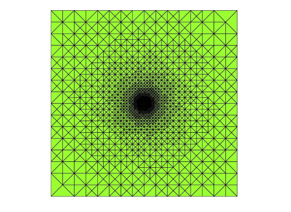
Figure 1. mesh generated by $\eta_{K}$.

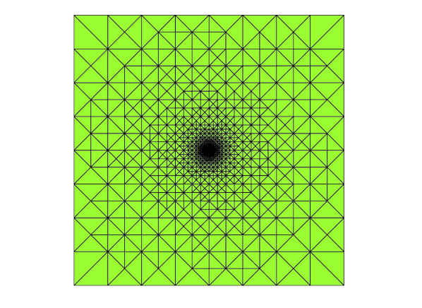
Figure 2. mesh generated by $\tilde{\eta}_{K}$.

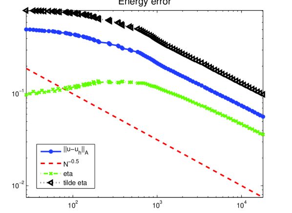
Figure 3. error and estimators on mesh generated by $\eta_{K}$.

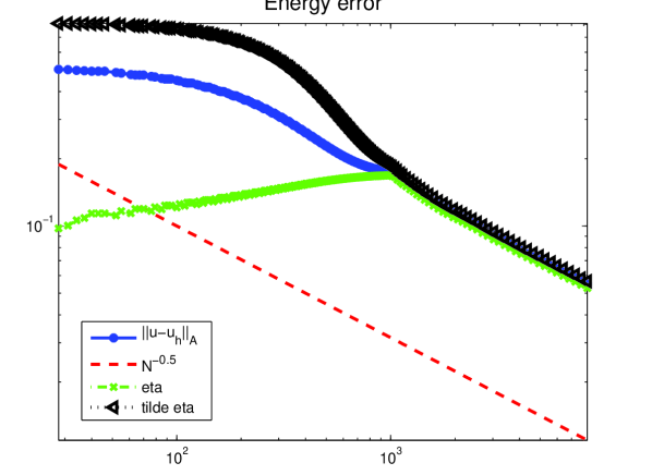
Figure 4. error and estimators on mesh generated by $\tilde{\eta}_{K}$.

Meshes generated by the standard and modified indicators, $\eta_{K}$ and $\tilde{\eta}_{K}$, are depicted respectively in Figures $1$ and $2$. Both the refinements are centered at the origin. There are 11974 and 5524 elements in the respective Figures 1 and 2. Hence, this test problem suggests that the modified indicator generates a much better mesh than the standard indicator even though the local efficiency bound of the modified indicator depends on the jump of the diffusion coefficient.

The comparisons of the true error and the estimators $\eta$ and $\tilde{\eta}$ on the meshes generated by the standard and modified indicators are shown in Figures 3 and 4, respectively. The slope of the log(dof)- log(error) for both the estimators on both the meshes are very close to $-1/2$, which indicates the optimal decay of the error with respect to the number of unknowns. The efficiency index is defined by

$$\mbox{eff-index}:=\displaystyle\frac{\mbox{estimator}}{|\!|\!|u-u_{h}|\!|\!|_{\Omega}}.$$

The efficinecy indices for the $\eta$ and $\tilde{\eta}$ are about $0.6404$ and $1.7469$ on the mesh generated by $\eta_{K}$ and about $0.9582$ and $1.0282$ on the mesh generated by $\tilde{\eta}_{K}$, respectively.

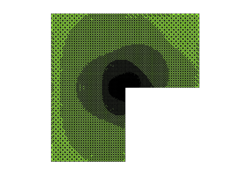
Figure 5. mesh generated by $\eta_{K}$ with solution jump

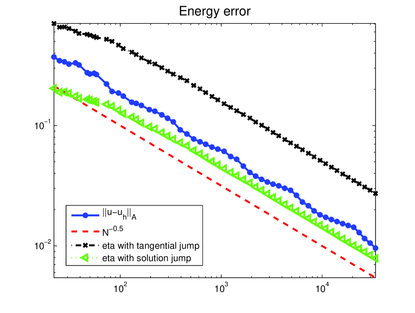
Figure 6. error and estimators on mesh generated by $\eta_{K}$

Our numerical results also show that our standard estimator using the edge solution jump is more accurate than the existing estimators using the edge tangential jump. To illustrate this fact, we present numerical results for a test problem [16]: a Poisson equation defined on the L-shaped domain $\Omega=(-1,\,1)^{2}\setminus[0,\,1]\times[-1,\,0]$ with the following exact solution

$$u(x,\,\theta)=r^{2/3}\sin\left(\displaystyle\frac{2\theta+\pi}{3}\right),\quad\theta\in[0,\,3\pi/2].$$

The stopping criteria is set as $tol\leq 0.0075$. The efficiency indices in the final step are $0.8205$ and $2.8423$ for the respective estimators with the edge solution and tangential derivative jumps. This indicates that our standard estimator is more accurate than the existing residual estimator (see Figure 6).

References

• [1] M. Ainsworth, Robust a posteriori error estimation for nonconforming finite element approximation, SIAM J. Numer. Anal., 42:6 (2005), 2320-2341.
• [2] M. Ainsworth, A posteriori error estimation for discontinuous Galerkin finite element approximation, SIAM J. Numer. Anal., 45:4 (2007), 1777-1798.
• [3] P. Becker, P. Hansbo, and M. G. Larson, Energy norm a posteriori error estimation for discontinuous Galerkin method, Comput. Meth. Appl. Mech. Engrg., 192 (2003), 723-733.
• [4] C. Bernardi and R. Verfürth, Adaptive finite element methods for elliptic equations with non-smooth coefficients, Numer. Math., 85 (2000), 579-608.
• [5] C. Carstensen, S. Bartels, and S. Jansche, A posteriori error estimates for nonconforming finite element methods, Numer. Math., 92 (2002), 233-256.
• [6] C. Carstensen, J. Hu, and A. Orlando, Framework for the a posteriori error analysis of the nonconforming finite elements, SIAM J. Numer. Anal., 45:1 (2007), 68-82.
• [7] Z. Cai, X. Ye, and S. Zhang, Discontinuous Galerkin finite element methods for interface problems: a priori and a posteriori error estimations, SIAM J. Numer. Anal., 49:5 (2011), 1761-1787.
• [8] Z. Cai and S. Zhang, Recovery-based error estimator for interface problems: conforming linear elements, SIAM J. Numer. Anal., 47:3 (2009), 2132-2156.
• [9] Z. Cai and S. Zhang, Flux recovery and a posteriori error estimators: conforming elements for scalar elliptic equations, SIAM J. Numer. Anal., 48:2 (2010), 578-602.
• [10] Z. Cai and S. Zhang, Recovery-based error estimator for interface problems: mixed and nonconforming elements, SIAM J. Numer. Anal., 48:1 (2010), 30-52.
• [11] Z. Cai and S. Zhang, Robust residual- and recovery a posteriori error estimators for interface problems with flux jumps, Numer. Methods for PDEs, 28:2 (2012), 476-491
• [12] Z. Cai and S. Zhang, Robust equilibrated residual error estimator for diffusion problems: conforming elements, SIAM J. Numer. Anal., 50:1 (2012), 151-170.
• [13] E. Dari, R. Duran, and C. Padra, Error estimations for nonconforming finite element approximations of the Stokes problem, Math. Comp., 64 (1995), 1017-1033.
• [14] E. Dari, R. Duran, C. Padra, and V. Vampa, A posteriori error estimators for nonconforming finite element methods, RAIRO Modél Anal. Numér., 30:4 (1996), 385-400.
• [15] M. Dryja, M. V. Sarkis, and O. B. Widlund, Multilevel Schwartz method for elliptic problems with discontinuous in three dimensions, Numer. Math., 72 (1996), 313-348.
• [16] H. Elman, D. Silvester, and A. Wathen, Finite Elements and Fast Iterative Solvers: With Applications in Incompressible Fluid Dynamics, Numer. Math. Sci. Comput., Oxford University Press, Oxford, UK, 2005.
• [17] V. Girault and P. A. Raviart, Finite Element Methods for Navier-Stokes Equations, Springer-Verlag, Berlin, 1986.
• [18] R. H. W. Hoppe and B. Wohlmuth, Element-oriented and edge-oriented local error estimators for nonconforming finite element methods, RAIRO Modél. Math. Anal. Numér., 30:2 (1996), 237-263.
• [19] R. B. Kellogg, On the Poisson equation with intersecting interfaces, Appl. Anal., 4 (1975), 101-129.
• [20] K. Y. Kim, A posteriori error analysis for locally conservative mixed methods, Math. Comp., 76 (2007), 43-66.
• [21] C. Lovadina and R. Stenberg, Energy norm a posteriori error estimates for mixed finite element methods, Math. Comp., 75 (2006), 1659-1674.
• [22] R. Luce and B. I. Wohlmuth, A local a posteriori error estimator based on equilibrated fluxes, SIAM J. Numer. Anal., 42:4 (2004), 1394-1414.
• [23] M. Petzoldt, A posteriori error estimators for elliptic equations with discontinuous coefficients, Adv. Comput. Math., 16 (2002), 47-75.
• [24] F. Schieweck, A posteriori error estimates with post-processing for nonconforming finite elements, ESAIM Math. Mod. Numer. Anal., 36:3 (2002), 489-503.
• [25] R. Verfürth, A Posteriori Error Estimation Techniques for Finite Element Methods, Oxford University Press, Oxford, United Kingdom, 2013.
• [26] M. Vohralík, Guaranteed and fully robust a posteriori error estimates for conforming discretizations of diffusion problems with discontinuous coefficients, J. Sci. Comput., 46:3 (2011), 397-438