Analysis of terrestrial planet formation by the Grand Tack model: System architecture and tack location

Abstract

The Grand Tack model of terrestrial planet formation has emerged in recent years as the premier scenario used to account for several observed features of the inner solar system. It relies on early migration of the giant planets to gravitationally sculpt and mix the planetesimal disc down to $\sim$1 AU, after which the terrestrial planets accrete from material left in a narrow circum-solar annulus. Here we have investigated how the model fares under a range of initial conditions and migration course-change (‘tack’) locations. We have run a large number of N-body simulations with a tack location of 1.5 AU and 2 AU and tested initial conditions using equal mass planetary embryos and a semi-analytical approach to oligarchic growth. We make use of a recent model of the protosolar disc that takes account of viscous heating, include the full effect of type 1 migration, and employ a realistic mass-radius relation for the growing terrestrial planets. Results show that the canonical tack location of Jupiter at 1.5 AU is inconsistent with the most massive planet residing at 1 AU at greater than 95% confidence. This favours a tack farther out at 2 AU for the disc model and parameters employed. Of the different initial conditions, we find that the oligarchic case is capable of statistically reproducing the orbital architecture and mass distribution of the terrestrial planets, while the equal mass embryo case is not.

1 Introduction

A successful physical model for the formation of the terrestrial planets is a long-standing problem (Tsiganis, 2015). The first physically plausible idea came from Safronov (1969) who suggested the earliest stage of accumulation of dust into larger bodies was caused by gravitational instability in a thin dust layer. Safronov (1969) showed that relative velocities between bodies are of the order of their escape velocity, so the largest body’s gravitational cross section is limited by the geometrical one, limiting growth. These findings were later used by Wetherill (1980), who showed the terrestrial planets coagulated from planetesimals, and that the formation of the these planets was linked with the evolution of the asteroid belt. Wetherill & Stewart (1989) elaborated that in a disc of planetesimals some would undergo runaway growth and form a sequence of planetary embryos. These embryos would then further collide to form the terrestrial planets.

These ideas were first rigorously tested by Kokubo & Ida (1996) who performed numerical simulations of a self-gravitating disc of planetesimals. They discovered that some objects in the disc underwent runaway growth, as was predicted, which resulted in a mixed population of protoplanets and planetesimals (Kokubo & Ida, 1998). The protoplanets underwent so-called oligarchic growth: all would be roughly equally spaced and be of similar mass as each vied for supremacy in accreting the last remaining planetesimals. The protoplanets (also dubbed ‘planetary embryos’) subsequently collide to form the terrestrial planets (Chambers, 2001).

Early simulations of terrestrial planet formation yielded estimates for a growth time scale of several tens of millions of years and overall results that showed the final terrestrial system would be assembled by 100 Myr (Chambers, 2001). Most of these early simulated systems, however, were found to suffer from an excess eccentricity and inclination of the final planets, but the inclusion of a large number of planetesimals to exert dynamical friction alleviated this concern (O’Brien et al., 2006). A further chronic and fundamental shortcoming with earlier simulations was that the output systematically yielded a far too massive Mars analogue. This predicament led Raymond et al. (2009) to investigate how the mass of Mars might depend on the orbital configuration of the giant planets. It was found that only the current spacing of the gas giants led to the capability of the model to produce a Mars analogue much less massive than Earth, but under the special condition that the eccentricities of the gas giants were higher than their current values. As such, Raymond et al. (2009) highlighted the unrealistic nature of the initial conditions required to explain Mars’ low mass, and left the problem as a lingering impasse to be solved later.

A potential solution presented itself in the work of Hansen (2009), who studied terrestrial planet formation with planetary embryos situated in a narrow annulus between 0.7 AU and 1 AU from the Sun. These initial conditions nicely reproduced the mass-semimajor axis relationship we have today, with two relatively large terrestrial-type planets book-ended by two much less massive ones. The main drawback of that study was that no mechanism was presented to gravitationally truncate the outer edge of the solid disc near 1 AU. The same could be said for the inner edge, so that no mechanism existed to create such a high-density, narrow annulus with which to explain the terrestrial worlds.

This quandary led Walsh et al. (2011) to propose the so-called Grand Tack scenario, wherein the early gas-driven coupled migration of Jupiter and Saturn sculpts the planetesimal disc and truncates it near 1 AU. The Grand Tack at least partially explains the formation of a high density region in the inner disc, although it cannot explain the existence of an inner cavity inside of roughly 0.7 AU. The inclusion of this scenario leads to a broad outline of how the early solar system evolved: First, Jupiter is assumed to form before Saturn, clear the gas in an annulus the width of which is comparable to its Hill radius, and undergo inward Type 2 migration (Lin & Papaloizou, 1986). The inward migration of Jupiter shepherds material towards the inner portion of the disc while also scattering other material outwards, to create an enhanced density region for terrestrial planet formation and that mixes planetesimals from the innermost and outer portions of the protoplanetary disc. Once Saturn grows to about half its current mass (Masset & Casoli, 2009), it is assumed to partially clear the disc in its vicinity, migrate rapidly at first to catch up with Jupiter, and subsequently get trapped in a mean-motion resonance near Jupiter, presumably the 2:3 (Masset & Snellgrove, 2001; Pierens & Raymond, 2011) but it may also have been the 2:1 (Pierens et al., 2014). In this process, these two giant planets clear the disc together. The torque from the interaction with the disc is stronger for a shorter separation between the planet and the disc edge. Since Jupiter and Saturn are interacting and Jupiter is more massive, it is reasonable to think that Saturn is pushed outwards by Jupiter’s perturbation, and the separation from the disc edge is smaller for Saturn than for Jupiter. Thus the torque on Saturn can be larger in spite of lower mass. The interaction with Jupiter prevents Saturn from creating a cleared annulus in the disc and gas from the outer disc flows past Saturn into the inner disc. If the gap-crossing disc gas flow is large enough, the Jupiter-Saturn pair can migrate outwards (Masset & Snellgrove, 2001; Pierens & Nelson, 2008). Consequently, the planets reverse their migration: they ’tack’ as a sail boat would change its direction by steering into and through the wind. Once the giant planets have completed this early migration phase, have left the inner solar system and settled in the vicinity of their present positions, terrestrial planet formation could proceed as before, but only (as advocated by Hansen (2009)) from material in a narrow circum-solar annulus. In this manner Walsh et al. (2011) successfully reproduced the mass-semimajor axis distribution of the inner planets if the reversal of Jupiter occurred at 1.5 AU because they truncated the inner edge of their planetesimal disc at 0.5 AU. A successful feature of their model is that it also accounts for the apparent compositional differences across the asteroid belt (DeMeo & Carry, 2014).

It is worth noting, however, that this step wise reconstruction of the early evolution of the planetary system has some pitfalls of varying severity. For example, the particular configuration and outward migration of the giant planets favoured by the Grand Tack is only supported for a narrow set of initial conditions (D’Angelo & Marzari, 2012) and is not universal (Zhang & Zhou, 2010). There may also be other pathways to produce such a high density region through a deficit of material near Mars (Izidoro et al., 2014), although this idea was recently undermined in a follow-up study (Izidoro et al., 2015). Lastly, up to this point the Grand Tack fails to reproduce the current mass and location of Mercury, most likely because dynamical models always truncate the disc near 0.5 AU or beyond. Clearly further study is needed in both the gas-driven evolution of the giant planets and the subsequent formation and evolution of the terrestrial planets to explain what we see in our own solar system.

With this in mind, we sought to scrutinise the Grand Tack model and its consequences over most of the age of the solar system, by running a large number of Grand Tack simulations with a range of initial conditions and varying tack locations. Our work also include d several dynamical effects that have hitherto been ignored. We report on the various methods that were employed to quantify whether or not Grand Tack successfully reproduces the observed dynamical features of the inner solar system and whether one set of initial conditions and tack location is more favourable than another.

This report is organised as follows. In Section 2 we introduce several additions to the original Grand Tack simulations of Walsh et al. (2011) and justify our choice of disc model and the inclusion of type 1 migration. Section 3 describes our initial conditions, while Section 4 describes our numerical methods. Section 5 explains our criteria for a set of simulations to successfully reproduce the current observed dynamical properties of the inner solar system. This is followed by Sections 6 and Section 7 where we describe the results of our numerical simulations. Section 8 is reserved for a discussion, and we draw our conclusions in Section 9.

2 Deviations from the original Grand Tack model

In addition to the simple reproduction of the Grand Tack scenario, for this study we also chose to employ a substantially different model for the protoplanetary disc than that used by Walsh et al. (2011). An explanation for this choice is provided below. We have also included the effect of type 1 embryo migration.

2.1 Protoplanetary disc

Walsh et al. (2011) employed the protoplanetary disc model of Morbidelli & Crida (2007), which in turn was based on the work of Guillot & Hueso (2006). The surface density of their disc profile is of the form $\Sigma(r)=\Sigma_{0}\exp(-r^{2}/R^{2})$, where $R\sim 200\,\,{\rm AU}$ is a scaling constant. This Gaussian profile of the surface density is markedly different from the oft-employed power law slopes found elsewhere in the literature e.g. Hartmann et al. (1998). The scaling constant at 1 AU is $\Sigma_{0}=100$ g cm^-2, which is much lower than the usual value of 1700–2400 g cm^-2 (Hayashi, 1981). Since the disc model of Morbidelli & Crida (2007) is not widely used and relies on a constant viscosity, $\nu$, rather than a constant $\alpha$-viscosity, we decided to make use of the disc model of Bitsch et al. (2015), which is based on the study by Hartmann et al. (1998). Bitsch et al. (2015) give fitting formulae to compute the disc’s surface density, temperature and scale height as a function of both heliocentric distance and time. Initially the disc’s gas surface density at 1 AU is 2272 g cm^-2 and the temperature is 576 K in the midplane so that the scale height at 1 AU is about 0.057 AU and the metallicity is equal to the solar value. This is higher than most traditional models have assumed and the higher temperature is caused by viscous heating. These fitting formulae are valid, however, as long as any embedded planet is not massive enough to significantly alter the disc structure, such as opening an annulus, and as long as the disc remains mostly unperturbed. This latter requirement may not be entirely true because of the proximity of Jupiter, whose presence imposes a change in the disc’s surface density and temperature. For a radiative disc, this change in the temperature profile will result in a change in the disc surface density, but for a viscous disc, which is the region we work in, this effect is less severe. Besides, a much lower disc temperature, caused by the influence of Jupiter, would mean that the ice line is close to 1 AU very early on, which is inconsistent with solar system formation (Matsumura et al., 2016). Here we adopt the disc of Bitsch et al. (2015) and set the $\alpha$ viscosity equal to 0.005, use a solar metallicity and a molecular weight of the gas of 2.3 amu (Bitsch et al., 2015). The gas surface density scales as $\Sigma(r)\propto r^{-\alpha}$ and the temperature profile is $T(r)\propto r^{-\beta}$, where $\alpha=1/2$ and $\beta=6/7$. These power law relations are accurate out to $\sim$5 AU, which is the region we are interested in, so we adopted these profiles throughout the disc. In Fig. 1 we plotted the evolution of the surface density (top) and the temperature bottom as a function of time and distance to the Sun. There is a very rapid decay for the first 1 Myr and a slower decay after that. After 5 Myr we photo-evaporate the disc away over the next 100 kyr.

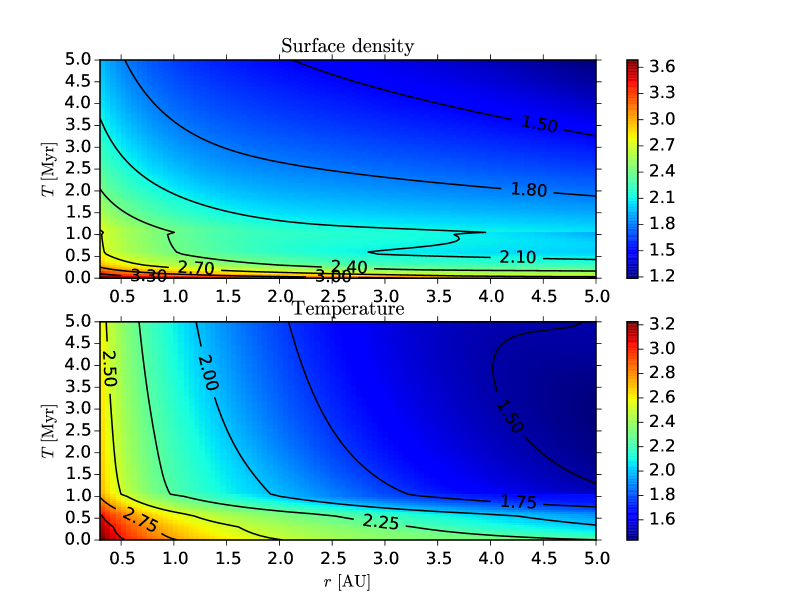
Figure 1: Contour plots of $\log(\Sigma/1\,{\rm g\,cm}^{-2})$ (top) and $\log(T/1\,{\rm K})$ (bottom) as a function of distance to the Sun (horizontal axis) and age in Myr (vertical axis).

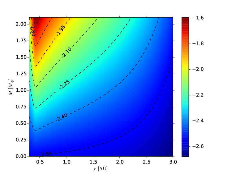
Figure 2: Contour plots of the normalised torque on a planetary embryo as a function of semi-major axis and mass.

2.2 Embryo migration

Although Walsh et al. (2011) decided not to include the effect of type 1 migration (Tanaka et al., 2002) on the planetary embryos, we decided to take it into account to determine whether (or not) it drastically affects the outcome of the simulations. For the migration prescription we follow Cresswell & Nelson (2008), which is partially based on the work of Tanaka et al. (2002). We chose not to employ the non-isothermal approach of Paardekooper et al. (2011) because generally none of the terrestrial planets are massive enough to begin outward migration apart from at the very late stages when the disc surface density is low. Thus, for simplicity, we shall adhere to the isothermal case. The specific decelerations experienced by the planetary embryos due to the disc on the eccentricity, inclination and semi-major axis are given by

$$\vec{a}_{e} = -2\frac{(\vec{v}\cdot\vec{r})}{r^{2}t_{e}}\vec{r},$$ (1)

$$\vec{a}_{i} = -\frac{v_{z}}{t_{i}}\vec{k},$$ (2)

$$\vec{a}_{m} = -\frac{\vec{v}}{t_{m}},$$ (3)

where $\vec{r}$ and $\vec{v}$ are the position and velocity vectors of the embryo, $\vec{k}$ is the unit vector in the $z$-direction, $v_{z}$ is the $z$-component of the velocity, and $t_{e}$, $t_{i}$ and $t_{m}$ are the time scales to damp the eccentricity, inclination and semi-major axis. The latter quantities depend in a complicated manner on the semi-major axis, eccentricity, inclination, surface density and temperature of the gas, and mass of the embryo. We refer the interested reader to Cresswell & Nelson (2008) and Tanaka et al. (2002) for details and for conversion to the cartesian frame. All of the above time scales are a function of the wave time, given by (Tanaka & Ward, 2004)

$$t_{\rm wav} = \Bigl{(}\frac{M_{\odot}}{m_{\rm emb}}\Bigr{)}\Bigl{(}\frac{M_{\odot}}{\Sigma r^{2}}\Bigr{)}\Bigl{(}\frac{c}{r\Omega_{\rm K}}\Bigr{)}^{4}\Omega_{\rm K}^{-1},$$ (4)

$$= \Bigl{(}\frac{M_{\odot}}{m_{\rm emb}}\Bigr{)}\Bigl{(}\frac{M_{\odot}}{\Sigma r^{2}}\Bigr{)}\Bigl{(}\frac{H}{r}\Bigr{)}^{4}\Bigl{(}\frac{r}{v_{\rm K}}\Bigr{)}$$

where we used $H/r=c/v_{\rm K}$, $\Omega_{\rm K}$ is the orbital frequency, $c^{2}=\gamma k_{\rm B}T/\mu m_{\rm p}$ is the sound speed, $v_{\rm K}$ is the orbital speed and $H$ is the scale height, $\gamma$ is the ratio of specific heats (taken as 7/5), $k_{\rm B}$ is the Boltzmann constant, $m_{\rm p}$ is the mass of the proton and $\mu$ is the molecular weight of the gas, assumed to be 2.3 amu. The value of $t_{\rm wav}$ depends sensitively on the slopes of the surface density and temperature profiles but the product $m_{\rm emb}t_{\rm wav}\propto a^{3/2-2\beta+\alpha}$ is much less sensitive and is what determines the migration rate of the embryos. We generally have $m_{\rm emb}t_{\rm wav}\sim a^{2/7}$ to $a^{2}$ for our disc profile and the minimum disc profile of Hayashi (1981) (which has $\alpha=3/2$ and $\beta=1/2$).

Walsh et al. (2011) included the first two deceleration contributions in equations (1-3) since these are tidal effects by the disc that damp the eccentricity and inclination, but they omitted the third (equation 3) which is in part responsible for the inward migration of the planetary embryos. For the disc that we have chosen we compute near 1 AU $t_{m}\sim 2\,(0.1~{}M_{\oplus}/m_{\rm emb})(2000~{}{\rm g}\,{\rm cm}^{-2}/\Sigma)$ Myr, so any inward migration that the embryos experience will likely be severely restricted because the migration time scale is longer than the disc lifetime and increases as the disc surface density decreases. However $t_{e}~{}\sim 21$ kyr for a Mars-sized body near 1 AU so the damping effect is a lot stronger than the migration. For the disc employed by Walsh et al. (2011) the migration and damping time scales are both at least an order of magnitude longer, so that their effects of type 1 migration are very weak.

To compare our migration times with earlier results, we note that for an Earth-sized body at 1 AU our nominal disc parameters yield $t_{\rm wav}\sim 1700$ yr and $t_{m}\sim 180$ kyr, which are much longer than the values of Tanaka et al. (2002) and Tanaka & Ward (2004) because our disc is initially hotter. The wave time scales as $(H/r)^{4}$ so that a factor of 1.5 in $H/r$ will result in a factor 5 in the migration time scale, while $t_{\rm m}\propto(H/r)^{2}$ so the effect of the disc temperature is weaker. As the disc evolves the temperature decreases, speeding up type 1 migration, but so does the surface density, slowing it down. In general, the effect of type 1 weakens with time.

Thus, the effect of type 1 migration should be relatively weak in our disc model compared to the traditional results of Tanaka et al. (2002) and Tanaka & Ward (2004). Apart from the migrating force, the eccentricity and inclination damping forces from the disc will also cause some inward migration of the embryos due to angular momentum loss, and we expect them to migrate inwards of the order of 0.1 AU over the lifetime of the disc. In Fig. 2 we plot a contour map of the normalised torque on the planetary embryos as a function of their distance to the Sun and their mass at time zero of the age of the disc. The normalised torque is $\Gamma_{\rm n}=\Gamma_{\rm tot}/\Gamma_{0}$ where $\Gamma_{0}=(m_{\rm emb}/M_{\odot})^{2}(r/H)^{2}(v/r)^{2}\Sigma$. The migration rate is then $\dot{r}=-2r\Gamma_{\rm tot}/L$, where $L$ is the orbital angular momentum (Tanaka et al., 2002). In all the disc models the definition of the torque is always inward.

3 Initial conditions

For this project we have run a large sample of numerical simulations of the Grand Tack scenario. These simulations are categorised into four large sets, with further subdivisions therein.

All simulations start with a high number of small planetesimals, planetary embryos, and the gas giants Jupiter and Saturn. We do not include Uranus and Neptune in any of the simulations, because they do not have any immediate effects on the formation of the terrestrial planets (Walsh et al., 2011). In all simulations we chose to not take account of the effect of Saturn’s mass growth. According to Walsh et al. (2011) and Jacobson & Morbidelli (2014), other effects, such as the radial evolution of Saturn and the gas giant migration time scale, did not substantially change the final terrestrial planet systems. Given the high number of free parameters, we decided to follow Walsh et al. (2011) to cases where Jupiter is assumed to have its current mass and is initially placed on a near-circular orbit at 3.5 AU. A fully-grown Saturn is placed in the 2:3 resonance with Jupiter at 4.5 AU. During the first 0.1 Myr, Jupiter and Saturn migrate from their initial locations (3.5 AU and 4.5 AU) to the tack locations (either 1.5 AU and 2.0 AU for Jupiter), respectively. For the next 5 Myr, Jupiter and Saturn migrate out to $\sim$ 5.4 AU and $\sim$ 7.5 AU, which are appropriate initial conditions for late giant planet migration models (Morbidelli et al., 2007). Walsh et al. (2011) demonstrated that the migration speed of the gas giants has almost no influence on the final architecture of the terrestrial system. We therefore used the same linear inward migration of the gas giants with a time-scale of 0.1 Myr, followed by outward migration via an exponential prescription with an e-folding time of 0.5 Myr. These time scales are comparable to the typical rate of Type 2 migration (Lin & Papaloizou, 1986).

To compare the effects of different formation models on the architecture of the terrestrial planets, we use various initial distributions of embryos and planetesimals.

3.1 Equal mass embryo initial conditions

For the first two large sets of simulations we employ the initial conditions of the embryos and planetesimals from Jacobson & Morbidelli (2014), but we use our model for the protoplanetary disc. These simulations were run because we want to directly compare the results of our modified simulations – employing a different protoplanetary disc, including type 1 migration and a realistic mass-radius relationship – with theirs. All of the simulations in this set use equal mass embryos initially situated between 0.7 AU and 3 AU. The embryos were embedded in a disc of planetesimals. The surface density of embryos and planetesimals both scaled with heliocentric distance as $r^{-3/2}$. Following Jacobson & Morbidelli (2014) the total mass ratio of embryos and planetesimals in this inner disc is either 1:1, 4:1 or 8:1, with the individual embryo masses being either 0.025, 0.05 or 0.08 $M_{\oplus}$. The equal mass embryo assumption appears to agree with a pebble-accretion scenario of embryo formation (Morbidelli et al., 2015)(Levison et al., 2015) rather than the more traditional oligarchic growth scenario (Kokubo & Ida, 1998), although which scenario is favoured is still under considerable debate. To mimic the coagulation evolution of the solids in the disc, we follow Chambers (2006) and calculate the age of the disc is 0.1 Myr when embryos have a mass of 0.025 $M_{\oplus}$, it is 0.5 Myr when the embryos have a mass of 0.05 $M_{\oplus}$ and 1 Myr when the embryos have a mass of 0.08 $M_{\oplus}$.

Following Jacobson & Morbidelli (2014) again, the total mass in solids in the inner disc (embryos and planetesimals) is 4.3 $M_{\oplus}$ when the total mass ratio between embryos and planetesimals is 1:1, 5.3 $M_{\oplus}$ when the mass ratio is 4:1 and 6.0 $M_{\oplus}$ when the mass ratio is 8:1. Jacobson & Morbidelli (2014) further argued these different initial disc masses were necessary to keep the post-migration mass in solids between 0.7 AU and 1 AU close to 2 $M_{\oplus}$. Therefore, the surface density in solids between these different initial conditions increases with increasing total embryo to planetesimal mass ratio. The number of planetary embryos ranged from 29 to 213 depending on their initial mass and total mass ratio. We kept the number of planetesimals at 2000, regardless of their total mass. The initial densities of the planetesimals and embryos was 3 g cm^-3 (Walsh et al., 2011). The permutations of these initial conditions results in nine individual sets of simulations.

Following Matsumura et al. (2016), for most of the simulations we also added an outer disc of planetesimals. This disc consists of 500 planetesimals with a total mass of 0.06 $M_{\oplus}$. These planetesimals are to some degree considered responsible for volatile delivery on the otherwise dry terrestrial planets Matsumura et al. (2016). The outer planetesimals are distributed between 5 AU and 9 AU. The eccentricities and inclinations of both embryos and planetesimals are randomly chosen from a uniform distribution between 0 and 0.01 and 0 to 0.5^∘. The other angular orbital elements were chosen uniformly at random from 0 to 360^∘. We ran two sets of these nine permutations, one with a tack at 1.5 AU as in Walsh et al. (2011), and one with a tack at 2 AU as described in Matsumura et al. (2016).

3.2 Oligarchic initial conditions

Apart from simulating the formation of the terrestrial planets from a disc of equal-mass embryos and planetesimals we also run a second set of simulations where the initial conditions are reminiscent of the traditional oligarchic growth scenario (Kokubo & Ida, 1998). To set up our simulations, we used the semi-analytical oligarchic approach of Chambers (2006). In that work, the mass of embryos increases up to their isolation mass as

$$m_{\rm p}(t)=m_{\rm iso}\tanh^{3}\Bigl{(}\frac{t}{\tau}\Bigr{)},$$ (5)

where $m_{\rm iso}=2\pi a\Sigma_{\rm s}b$ is the isolation mass at semi-major axis $a$ for embryos spaced $b$ AU apart embedded in a disc with solid surface density $\Sigma_{\rm s}$. Here $\tau$ is the growth time scale which is a complex function of the semi-major axis, embryo spacing, solid surface density and radii of planetesimals that accrete onto the embryos. The growth time scale is given by (Chambers, 2006)

$$\tau=\frac{2e_{\rm Hi,eq}^{2}}{A}$$ (6)

where

$$e_{\rm Hi,eq}^{2} = 2.7^{2}\Bigl{(}\frac{r_{\rm c}\rho}{bC_{D}a\rho_{\rm gas}}\Bigr{)}^{2/5}$$

$$= 17.5\Bigl{(}\frac{r_{\rm c}}{10\,{\rm km}}\Bigr{)}^{2/5}\Bigl{(}\frac{\rho}{2.5\,{\rm g~{}cm}^{-3}}\Bigr{)}^{2/5}\Bigl{(}\frac{b}{10\,R_{H}}\Bigr{)}^{-2/5}\Bigl{(}\frac{\rho_{\rm gas,0}}{1.4\times 10^{-9}\,{\rm g~{}cm}^{-3}}\Bigr{)}^{-2/5}\Bigl{(}\frac{a}{1\,{\rm AU}}\Bigr{)}^{2/5\alpha+1/5-1/5\beta},$$

assuming the drag coefficient $C_{D}=2$ and

$$\frac{1}{A} = \frac{b^{1/2}P\rho^{1/3}M_{\odot}^{1/6}}{31.7\Sigma_{\rm s}^{1/2}}$$ (8)

$$= 30.1~{}{\rm kyr}\Bigl{(}\frac{b}{10\,R_{H}}\Bigr{)}^{1/2}\Bigl{(}\frac{\rho}{2.5\,\rm{g~{}cm}^{-3}}\Bigr{)}^{1/3}\Bigl{(}\frac{\Sigma_{s}}{10\,\rm{g~{}cm}^{-2}}\Bigr{)}^{-1/2}\Bigl{(}\frac{a}{1\,\rm{AU}}\Bigr{)}^{3/2-1/2\alpha}M_{\odot}^{1/6}.$$ (9)

Here $\alpha$ is the slope of the solid surface density, $\beta$ is the slope of the temperature, $\rho_{\rm gas,0}$ is the gas density at 1 AU in the midplane, $r_{\rm c}$ is the radius of planetesimals, $\rho$ is their density and $P$ is the orbital period (Chambers, 2006). Here we used the fact that the gas density profile depends on the scale height and gas surface density which yields $\rho_{\rm g}\propto a^{-\alpha-3/2+1/2\beta}$. Combining all the above gives

$$\tau = 527\,{\rm kyr}\,\Bigl{(}\frac{b}{10\,R_{H}}\Bigr{)}^{1/10}\Bigl{(}\frac{\Sigma_{s}}{10\,{\rm g\,cm}^{-2}}\Bigr{)}^{-1/2}\Bigl{(}\frac{\rho}{2.5\,{\rm g\,cm}^{-3}}\Bigr{)}^{11/15}\Bigl{(}\frac{r_{\rm c}}{10\,{\rm km}}\Bigr{)}^{2/5}$$ (10)

$$\times \Bigl{(}\frac{\rho_{\rm gas,0}}{1.4\times 10^{-9}\,{\rm g~{}cm}^{-3}}\Bigr{)}^{-2/5}\Bigl{(}\frac{a}{1\,{\rm AU}}\Bigr{)}^{17/10-1/10\alpha-1/5\beta}M_{\odot}^{1/6},$$

where $\Sigma_{s}$ is the solid disc surface density at 1 AU and we assumed that $\Sigma_{\rm s}$ has the same radial dependence as the gas surface density. This derived value of $\tau$ and the subsequent growth of any embryo near 1 AU agrees well with Figure 1 in Chambers (2006). Adopting $\alpha=3/2$ and $\beta=6/7$, the above equation is a reasonably steep function of semi-major axis at a fixed epoch because $\tau\propto a^{193/140}\sim a^{1.38}$. When we use the typically-assumed value $\beta=1/2$ then we have $\tau\propto a^{3/2}$. At the Earth’s location the growth time for nominal parameters is $\sim$600 kyr while at Mars’ current orbit the growth time is $\sim$1 Myr. This is somewhat shorter than that advocated by Dauphas & Pourmand (2011) but is within error margins and is easily increased to 1.8 Myr assuming accretion was caused by planetesimals of $\sim$50 km.

We constructed our initial disc of embryos and planetesimals as follows. First, we computed the total mass in solids between 0.7 AU and 3 AU assuming the surface density in solids is $\Sigma_{s}=7$ g cm${}^{-2}(a/1\,{\rm AU})^{-3/2}$. This setup is just the minimum mass solar nebula (Hayashi, 1981). Second, following Ogihara & Ida (2009), we subsequently increased the solid density by a factor of 3 at the ice line, assumed to be static at 2.7 AU. Third, based on the results of Kokubo & Ida (1998), we imposed a spacing of 10 mutual Hill radii for the embryos, with the spacing computed assuming the embryos had their isolation masses. In other words, the semi-major axis of embryo $n$ is $a_{n}=a_{n-1}[1+b(2m_{\rm iso}/3M_{\odot})^{1/3}]$ so that the embryo spacing nearly follows a geometric progression. Following Chambers (2006) we assumed a planetesimal size of 10 km in computing the growth time scale of the embryos. Last, we entered the epoch at which Jupiter was assumed to have fully formed and began migrating. This was either 0.5 Myr, 1 Myr, 2 Myr or 3 Myr. Most embryos have only reached a fraction of their isolation mass and the remaining mass within their feeding annulus of 10 Hill radii taken up by planetesimals, with each planetesimal having a mass of 10^-3 $M_{\oplus}$. The eccentricities of the embryos and planetesimals followed a Rayleigh distribution with scale parameter equal to $(m_{\rm p}/3M_{\odot})^{1/3}$. The inclinations also followed a Rayleigh distribution with a scale parameter equal to half of that of the eccentricities. The other angles were chosen uniformly at random between 0 and 360^∘. All embryos and planetesimals had an initial density of 3 g cm^-2. The most distant embryo was typically at 2.6 AU.

4 Methodology

The gas giants, planetary embryos and planetesimals are simulated with the symplectic SyMBA integrator (Duncan et al., 1998) with a time step of 0.02 yr for 150 Myr. The end time of the simulations corresponds closely to the end of the purported Late Veneer (see next section). The migration of the gas giants was mimicked through fictitious forces described in Walsh et al. (2011). We first employed the same gas profile as Walsh et al. (2011) with two large dips around the gas giants, which migrated inwards with these planets, but we modified the gas density profile during the computation so that it followed the $\Sigma(r)\propto r^{-1/2}$ surface density law of Bitsch et al. (2015) rather than the Gaussian of Walsh et al. (2011). The initial total mass of the disc was approximately 0.05 $M_{\odot}$. The initial disc profile is depicted in Fig. 3. The blue line is the disc from Bitsch et al. (2015), whereas the red one is from Walsh et al. (2011). Jupiter is assumed to be at 3.5 AU and the disc age is zero.

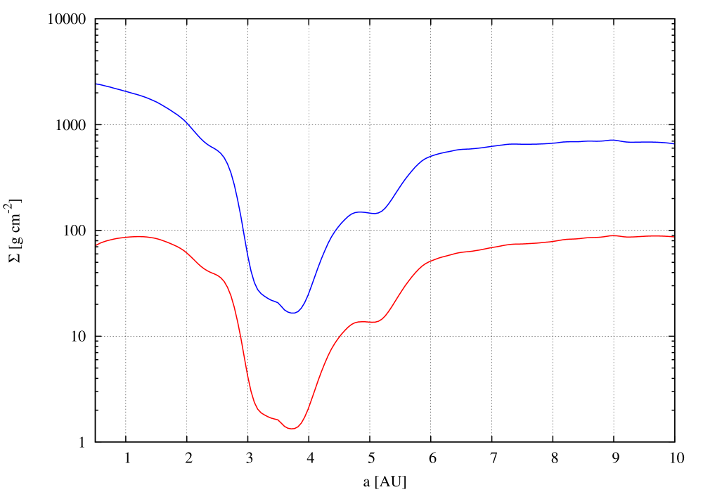
Figure 3: Density profile of the gas disc with Jupiter at 3.5 AU and the disc age is zero. The blue line is the disc we employed from Bitsch et al. (2015) while the red line is the disc profile of Walsh et al. (2011).

The planetary embryos experienced tidal damping of their eccentricities and inclinations and a negative torque from the gas disc as described in Section 2, and the orbits of the planetesimals evolve due to gas drag using the methods of Brasser et al. (2007). Following Walsh et al. (2011) and Jacobson & Morbidelli (2014) for the purpose of the gas drag, we assumed each planetesimal had a radius of 50 km. These planetesimals are larger than the 10 km size assumed for oligarchic growth because we wanted to compare our simulations directly with Jacobson & Morbidelli (2014). The gas drag routines of Brasser et al. (2007) were modified slightly to allow for a smooth transition between regimes when the Knudsen number crossed 1. We now have the following scheme:

• When $\mathcal{M}>2.727$, $C_{D}=2$ for all $\mathcal{K}$ and $\mathcal{R}$;

• When $\mathcal{R}>1000$, $C_{D}=0.44+0.2098\mathcal{M}^{2}$ for $\mathcal{M}<2.727$;

• When $\mathcal{R}<1000$

  $$C_{D}=0.2689\mathcal{M}^{2}+\frac{24}{\mathcal{R}}\Bigl{[}1-\Bigl{(}\frac{\mathcal{M}}{2.727}\Bigr{)}^{2}\Bigr{]}\frac{1+0.15\mathcal{R}^{0.687}}{\sqrt{\mathcal{K}^{2}+1}}.$$ (11)

Here $\mathcal{M}$, $\mathcal{K}$ and $\mathcal{R}$ are the Mach, Knudsen and Reynold numbers of the planetesimals, and $C_{D}$ is the drag coefficient (Brasser et al., 2007). In addition to the drag coefficient routine, we made one further modification to the code.
SyMBA treats collisions between bodies as perfect mergers, preserving their density. This works well in most circumstances, but given that the mean density of Earth is 5.5 g cm^-2 and not 3 g cm^-2, we implemented the mass-radius relationship of Seager et al. (2007) to make sure that the final planets have radii comparable to the current terrestrial planets so that their collisional cross sections are not artificially large. The relation we employed was

$$\log\Bigl{(}\frac{R_{p}}{3.3\,R_{\oplus}}\Bigr{)}=-0.209+\frac{1}{3}\log\Bigl{(}\frac{M_{p}}{5.5\,M_{\oplus}}\Bigr{)}-0.08\Bigl{(}\frac{M_{p}}{5.5\,M_{\oplus}}\Bigr{)}^{0.4},$$ (12)

where $R_{p}$ and $M_{p}$ are the radius and mass of the planetary embryo. This relation fits Mars, Venus and Earth well.
During the simulations we computed the mutual gravity between gas giants and embryos, but the planetesimals were not able to affect each other. This approximation was used to keep the CPU time within reasonable limits, and is justified because Jupiter clears the disc beyond 1 AU in 100 kyr. Planets and planetesimals were removed once they were farther than 100 AU from the Sun (whether bound or unbound) or when they collided with a planet or ventured closer than 0.2 AU from the Sun.

For each permutation of the equal mass embryo initial conditions of Jacobson & Morbidelli (2014) we ran 16 simulations (144 for each tack location), while for the oligarchic initial conditions we ran 16 simulations for each starting epoch (64 for each tack location). In total, we ran 416 simulations, categorised in Table 1. The oligarchic simulations were run at the Centre for Computational Astrophysics at the National Astronomical Observatory of Japan, while the others were run at the Earth Life Science Institute at Tokyo Institute of Technology.

	Equal mass embryos
Embryo mass [$M_{\oplus}$]	$M_{\rm emb}:M_{\rm pl}$	Tack location	Migration epoch [Myr]
0.025	1:1, 4:1 or 8:1	1.5 AU or 2 AU	0.1
0.05	1:1, 4:1 or 8:1	1.5 AU or 2 AU	0.5
0.08	1:1, 4:1 or 8:1	1.5 AU or 2 AU	1
	Oligarchic
	Migration epoch [Myr]	Tack location
Oligarchic	0.5	1.5 AU or 2 AU
Oligarchic	1	1.5 AU or 2 AU
Oligarchic	2	1.5 AU or 2 AU
Oligarchic	3	1.5 AU or 2 AU

Table 1: Summary of the individual sets of simulations. For each set of initial conditions we ran 16 simulations.

5 A measure of success

According to its founders, the Grand Tack model has booked several successes. These include, but are not limited to: the ability to reproduce the mass-orbit distribution of the terrestrial planets (Walsh et al., 2011) (though mostly only for Venus, Earth and Mars), the compositional gradient and total mass of the asteroid belt (Walsh et al., 2011), the growth time scale of the terrestrial planets (Jacobson & Walsh, 2015) and in some cases the angular momentum deficit (AMD), spacing and orbital concentration of the terrestrial planets (Jacobson & Morbidelli, 2014), and possibly the timing of the Moon-forming impact (Jacobson et al., 2014). Some of these deserve further discussion before we outline our criteria for assigning success or failure to the individual simulations and the model itself.

Jacobson et al. (2014) use simulations of terrestrial planet formation based on the Grand Tack model to place constraints on the time of the Moon-forming impact (a.k.a. Giant Impact or GI). They do this by requiring that, after the GI, the Earth subsequently accreted a further 0.5% of its mass, which they claim is the best estimate compatible with the fraction of highly siderophile elements in the mantle used to account for the Late Veneer (Walker, 2009). From their simulations they arrive at a timing of 95$\pm$32 Myr. This is in agreement with the preferred Moon-forming time from hafnium-tungsten and samarium-neodymium geochronology, though on the higher end (Kleine et al., 2005; Touboul et al., 2007). It is also in agreement with recent dynamical modelling and ^40-39Ar age compilations for the HED meteorites that likely originate from asteroid 4 Vesta (Bottke et al., 2015). In most of the simulations presented by Jacobson & Morbidelli (2014), however, the last giant impact occurs much earlier than their preferred value. O’Brien et al. (2014) pointed out that such an early impact violates the constraint posed by the amount of highly siderophile elements in the Earth’s mantle used to define the Late Veneer in the first place. That said, a late accretion of 1% is still entirely within reason, and it may have been even higher: Albarède et al. (2013) argue that upwards of 4% of Earth’s mass was added to the planet by the Late Veneer. Their arguments are based on the timing and amount of water delivery, and the vaporisation of volatiles during accretion, throughout which a high fraction of impactor material is lost. Such a substantial amount of post-giant impact accretion would naturally push the epoch of the Moon-forming impact much further back in time, and leaves the timing issue once again wide open. A different approach or chronometer may be needed.

Marty (2012) argues for an Earth formation time shorter than 50 Myr. In a subsequent study Avice & Marty (2014) use iodine, plutonium and xenon isotopic data to suggest that the closure time of the Earth’s atmosphere is $40^{+20}_{-10}$ Myr, which would naturally coincide with the Moon-forming event. The formation time suggested by Avice & Marty (2014) is in excellent agreement with the hafnium-tungsten dates of Kleine et al. (2005) (40$\pm$10 Myr), but on the lower end of that advocated by Touboul et al. (2007) (62${}^{+92}_{-30}$ Myr) and Halliday (2008) (70-100 Myr). In summary, the timing of the Moon-forming event is still a topic of ongoing debate. It appears that radiogenic dating results in an earlier GI time than suggested by the simulations of Jacobson et al. (2014), although the simulation results depend sensitively on the assumed amount of subsequent accretion. Most of the reported ages agree within error bars, but the range remains tens of millions of years.

Since individual simulations are chaotic and show a great variety in outcomes (Jacobson & Morbidelli, 2014), we impose criteria the model must adhere to, which are listed below. In what follows, we define the Mercury, Venus, Earth and Mars analogues to have masses and semi-major axes within the ranges $(0.025\,M_{\oplus}<m<0.1\,M_{\oplus},0.27\,\,{\rm AU}<a<0.5\,\,{\rm AU})$, $(0.4\,M_{\oplus}<m_{p}<1.2\,M_{\oplus},0.55\,\,{\rm AU}<a<0.85\,\,{\rm AU})$, $(0.5\,M_{\oplus}<m_{p}<1.5\,M_{\oplus},0.85\,\,{\rm AU}<a<1.15\,\,{\rm AU})$ and $(0.05\,M_{\oplus}<m_{p}<0.15\,M_{\oplus},1.3\,\,{\rm AU}<a<1.7\,\,{\rm AU}$). We require that objects in the region of the asteroid belt have their perihelia $q>1.6$ AU and their aphelia $Q<4.5$ AU. We want to add a note of caution. Since we employ initial conditions very similar to Walsh et al. (2011) and Jacobson & Morbidelli (2014) we expect to have a very low probability of reproducing the mass and semi-major axis of Mercury. One may then argue we should only base our analysis on the other three terrestrial planets, but we decided against doing so.

Chambers (2001) introduced several quantities which describe the general dynamical properties of a planetary system. These are: 1) the AMD, given by

$${\rm AMD}=\frac{\sum_{k}\mu_{k}\sqrt{a_{k}}(1-\sqrt{1-e_{k}^{2}})\cos i_{k}}{\mu_{k}\sqrt{a_{k}}}$$ (13)

where $\mu_{k}=m_{k}/M_{\odot}$. Second is the fraction of mass in the most massive planet ($S_{m}$). Third is a concentration parameter ($S_{c}$), given by

$$S_{c}={\rm max}\Bigl{(}\frac{\sum_{k}\mu_{k}}{\sum_{k}\mu_{k}[\log(a/a_{k})]^{2}}\Bigr{)},$$ (14)

and last, a mean spacing parameter ($S_{H}$), which is

$$S_{H}=2\sum_{k=1}^{N-1}\frac{a_{k+1}-a_{k}}{a_{k+1}+a_{k}}\Bigl{(}\frac{\mu_{k+1}+\mu_{k}}{3}\Bigr{)}^{-1/3}.$$ (15)

Unlike Chambers (2001) we use the mutual Hill sphere as the spacing unit. Ultimately we invoke the following criteria to determine success or failure of the Grand Tack model: statistically the resulting terrestrial systems must have their median AMD lower than the current value, a concentration parameter 107$\pm$67 (2$\sigma$), a mean spacing in Hill radii of 45$\pm$12 (2$\sigma$), a mass parameter $>0.5$, produce at least one Mars analogue (or a probability in excess of 5% for a whole set) and the most massive planet must have a greater than 5% probability of residing at 1 AU i.e. the cumulative semi-major axis distribution of the most massive planet must be lower than 0.95 at 1 AU. The ranges in the listed values of $S_{c}$ and $S_{H}$ are computed using a Monte Carlo method adopting the range of masses and semi-major axes of our terrestrial planet analogues stated above.

6 Results: Tack at 1.5 AU

In this section we present the results of our numerical simulations.

6.1 Equal mass embryos

We have run the same simulations as Jacobson & Morbidelli (2014) in order to compare our results directly with theirs, and to determine whether a different protoplanetary disc model, realistic mass-radius relationship and inclusion of type 1 migration will substantially change the properties of the resulting planets. Generally we find that most of our results are in good agreement. We shall not give a full comparison, but a systematic overview and highlight some similarities and differences.

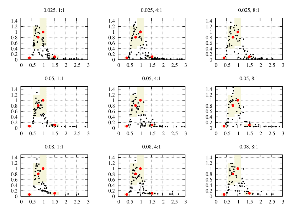
Figure 4: The final mass of the terrestrial planets [$M_{\oplus}$] versus their semi-major axis [AU]. The text above the panels indicates the embryo mass in Earth masses and the ratio of the total embryo to planetesimal mass. Beige regions indicate the range of our terrestrial planet analogues. Equal-mass embryo initial conditions with a tack at 1.5 AU.

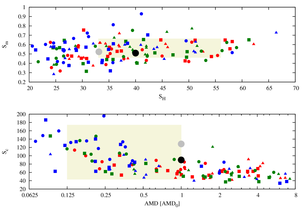
Figure 5: Top panel: Scatter plot of the spacing parameter $S_{H}$ vs the mass parameter $S_{m}$. Red symbols correspond to simulations with an initial embryo mass of 0.025 $M_{\oplus}$, green to initial embryo mass of 0.05 $M_{\oplus}$ and blue to initial embryo mass of 0.08 $M_{\oplus}$. Bullets are for simulations with a total embryo to planetesimal mass ratio of 1:1, squares are for a 4:1 mass ratio and triangles for an 8:1 mass ratio. Bottom: Scatter plot of concentration parameter $S_{c}$ vs normalised AMD. Equal-mass embryo conditions with a tack at 1.5 AU.

In Fig. 4 we compare the mass of each terrestrial planet that formed in our simulation versus their semi-major axis. The actual terrestrial planets are depicted as red bullets. For the most part our results comport with Figure 1 in Jacobson & Morbidelli (2014). In our simulations, however, the peak of the distribution is situated near Venus’ current location while the region near Earth is empty in comparison. This is not the case for Jacobson & Morbidelli (2014) where the peak is in between these planets, encompasses both, and is probably caused by early type 1 migration of the embryos. The mean semi-major axis and mass of the most massive planet in our simulations are $\langle a_{h}\rangle=0.769\pm 0.109$ AU and $\langle m_{h}\rangle=0.969\pm 0.189$ $M_{\oplus}$, with almost no variation within error bars as a function of either embryo seed mass or total embryo to planetesimal mass ratio. Thus our Venus analogue is almost always more massive than the Earth analogue, and, with more than 95% confidence, the position of the most massive planet is inconsistent with a location at 1 AU. This result is inconsistent with Jacobson & Morbidelli (2014) and we attribute this difference to our use of a distinctive model for the protoplanetary disc that has a a generally higher surface density, which causes stronger tidal damping, the inclusion of type 1 migration, and smaller planetary radii. Indeed, any material that is shepherded inwards by Jupiter will be at high eccentricity, which will be damped by interaction with the gas disc, which in turn will cause further inward migration since our gas disc has a higher surface density and a stronger damping than Jacobson & Morbidelli (2014). We emphasise that the inward migration caused by the damping forces is generally stronger than the direct effect of the type 1 term, so that even using the non-isothermal prescription of Paardekooper et al. (2011) would not substantially change the outcome.

In summary, our setup causes a peak density in solids near Venus’ current position rather than in between Earth and Venus as in Jacobson & Morbidelli (2014). For this reason we ran another set of simulations with a tack location at 2 AU rather than the typical 1.5 AU to determine whether that would produce more Earth analogues. We also report a similar low success to Jacobson & Morbidelli (2014) in producing Mercury analogues which, like them, we attribute to the initial conditions.

Embryo mass [$M_{\oplus}$]	$\langle n\rangle$	$\langle S_{c}\rangle$	$\langle$ AMD $\rangle$	$\langle S_{H}\rangle$
0.025	5.0 $\pm$ 1.1	66 $\pm$ 16	2.2 $\pm$ 2.2 (1.5)	40 $\pm$ 11
0.05	4.4 $\pm$ 1.3	71 $\pm$ 29	2.6 $\pm$ 3.3 (1.5)	40 $\pm$ 11
0.08	3.7 $\pm$ 1.0	97 $\pm$ 53	1.6 $\pm$ 3.1 (0.35)	34 $\pm$ 10
$M_{\rm emb}:M_{\rm pl}$	$\langle n\rangle$	$\langle S_{c}\rangle$	$\langle$ AMD $\rangle$	$\langle S_{H}\rangle$
1:1	4.1 $\pm$ 1.1	101 $\pm$ 47	1.1 $\pm$ 1.5 (0.37)	37 $\pm$ 13
4:1	4.8 $\pm$ 1.2	72 $\pm$ 33	2.0 $\pm$ 3.0 (1.0)	37 $\pm$ 10
8:1	4.3 $\pm$ 1.4	62 $\pm$ 19	3.3 $\pm$ 3.4 (2.11)	40 $\pm$ 10

Table 2: Properties of the terrestrial systems with a tack at 1.5 AU and equal-mass embryos. We list the average number of planets, concentration parameter, AMD and average spacing with their standard deviations. Since the AMD distribution usually has a long tail, we list the median value in parentheses.

How do the resulting planets fare otherwise? In Fig. 5 we plot the spacing parameter $S_{H}$ versus mass parameter $S_{m}$ in the top panel and concentration parameter $S_{c}$ versus normalised AMD (normalised to the current value) in the bottom panel. The typical value of $S_{c}$ decreases with AMD because the higher eccentricities force the planets to be wider apart if they are to remain stable. In this figure and the ones that follow, red symbols correspond to simulations with an initial embryo mass of 0.025 $M_{\oplus}$, green to initial embryo mass of 0.05 $M_{\oplus}$ and blue to initial embryo mass of 0.08 $M_{\oplus}$. Bullets are for simulations with a total embryo to planetesimal mass ratio of 1:1, squares are for a 4:1 mass ratio and triangles for an 8:1 mass ratio. The large black bullet denotes the current terrestrial system while the grey bullet is for the system consisting of only Venus, Earth and Mars. The beige regions denote 2$\sigma$ regions around the mean values of $S_{H}$, $S_{m}$ and $S_{c}$. The scaled AMD range was chosen not to exceed 1 because it will increase with time (Brasser et al., 2013; Laskar, 2008); the lower limit was chosen somewhat arbitrarily. Roughly 40% of all simulations fall in either one of the beige regions, though only 10% fall in both regions simultaneously. The results are summarised in Table 2. We reproduce the trend of Jacobson & Morbidelli (2014) that the AMD increases with a decrease in total planetesimal mass, though not with initial embryo mass. Jacobson & Morbidelli (2014) favour the cases with high embryo to planetesimal mass ratio, but the high resulting AMD is inconsistent with the dynamical evolution of the terrestrial planets (Brasser et al., 2013; Laskar, 2008). Jacobson & Morbidelli (2014) acknowledge the high AMD is a potential problem but suggest that fragmentation during embryo-embryo collisions could produce enough debris to damp the AMD through dynamical friction. It is not clear whether this can be sustained if collisional grinding is important. Further study is needed to support or deny this claim.

The terrestrial system consists of four planets. We find that the average final number of planets decreases with initial embryo mass and is mostly independent of the initial total mass ratio between the planets and embryos. The relatively high number of planets with low embryo seed mass is most likely skewed by stranded embryos in the asteroid belt or near Mars’ current position. The concentration parameter $S_{c}$ increases with more massive embryos but decreases for a lower planetesimal mass, most likely because the AMD is higher and the planets need to be spaced farther apart to remain dynamically stable.

We define the average probability of producing a terrestrial planet analogue as the fraction of planets in the designated mass-semimajor axis bin divided by the total number of produced planets. For a Venus analogue this is $24\%\pm 7\%$, for an Earth analogue it is $10\%\pm 3\%$ and for a Mars analogue it is $10\%\pm 4\%$. All of these values are above the 5% threshold, but we see an over-abundance of Venus analogues consistent with the density pileup reported earlier. We produced a total of two Mercury analogues (out of 635 planets).

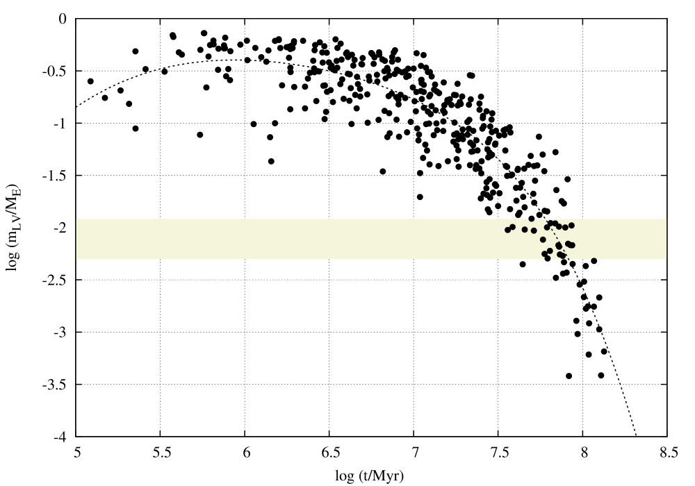
Figure 6: The last giant impact as a function of time versus subsequent accreted mass. The beige region comprises the amount constrained by highly siderophile elements in the Earth. Equal-mass embryo initial conditions with a tack at 1.5 AU.

Thus far it appears that the only difference between our results and Jacobson & Morbidelli (2014) is the peak of the mass distribution being closer to the Sun than theirs, most likely because of our different disc model. Our results differ as well when we investigate the timing of the Moon-forming impact. Following Jacobson et al. (2014) and Jacobson & Morbidelli (2014) again we compute the total amount of mass accreted by each planet between its last giant impact and the end of the simulation. We then plot this with a high-order polynomial best fit. The approximate timing of the Moon-forming impact is the intersection of the fit and some assumed Late Veneer mass (Jacobson et al., 2014), which is at most a few percent of an Earth mass (Albarède et al., 2013). The lower the amount of assumed late accreted mass, the later the giant impact had to occur because less mass had to have been around to impact the Earth afterwards.

We plot our results in Fig. 6, and obtain a best-fit value of 64 Myr for the timing of the Moon-forming event assuming 1% subsequent accretion. This is in good agreement with the Hf-W results from Kleine et al. (2005) and Touboul et al. (2007) but also sooner than what was suggested in the simulations of Jacobson et al. (2014). The difference in timing is most likely caused by us considering an accreted Late Veneer mass of 1% rather than 0.5%. However, the range of mass accreted after the giant impact is rather large. From the figure it is clear that this impact could have occurred anywhere between 30 Myr and 120 Myr, given the range of late accretion mass and uncertainties in the fit. Therefore we do not think that our simulations, or others such as Jacobson et al. (2014) for that matter, can confidently predict the timing of the Moon-forming event with this method.

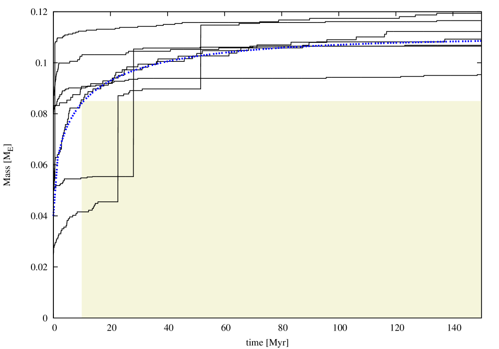
Figure 7: Evolution of mass with time for several Mars analogues. The beige region should be avoided because the formation time is inconsistent with the Hf-W chronometer (Nimmo & Kleine, 2007). The blue curve is a Weibull cumulative distribution with e-folding time $\tau=10$ Myr, stretching parameter $\beta=0.5$ and embryo seed mass 0.04 $M_{\oplus}$.

Another issue that requires attention is the growth of Mars. Jacobson & Morbidelli (2014) conclude that it is very difficult to reproduce the rapid growth of Mars as advocated by Dauphas & Pourmand (2011). Figure 7 shows the evolution of the mass of several Mars analogues produced in our simulations as a function of time. The beige region should be avoided because the growth rate in this region is inconsistent with the Hf-W chronometer of Mars’ formation (Nimmo & Kleine, 2007). The blue dashed curve shows a stretched exponential growth function $m\propto m_{\rm Mars}(1-\exp[-(t/\tau)^{\beta}]$). We fit a seed mass of 0.04 $M_{\oplus}$, stretching parameter $\beta\sim 0.5$ and e-folding time $\tau\sim 10$ Myr. These values are nearly identical to the growth of Earth and Venus (Jacobson & Walsh, 2015). Some Mars analogues experience early giant impacts with other embryos, substantially increasing their mass, but even then the final growth is slow and is inconsistent with the rapid growth advocated by Dauphas & Pourmand (2011), though still within limits of the Hf-W chronology of Nimmo & Kleine (2007).

One last thing that has not been actively reported by either Walsh et al. (2011), Jacobson & Morbidelli (2014) or O’Brien et al. (2014) is the amount of remaining mass in planetesimals. At the end of our simulations, we typically have a remnant mass in planetesimals of 0.051 $M_{\oplus}$$\pm$0.027 $M_{\oplus}$, which is comparable to the total mass required to reproduce the Late Veneer (Raymond et al., 2013). The remnant mass depends on the original total mass ratio between planetary embryos and planetesimals. The simulations with an initial 1:1 ratio have a typical final mass of 0.08 $M_{\oplus}$ while the 8:1 simulations typically have 0.01 $M_{\oplus}$. The decay follows a stretched exponential with best fits $\beta=0.43\pm 0.03$ and $\beta\log\tau=0.40\pm 0.04$, comparable to the results of Jacobson & Walsh (2015). Thus, after 150 Myr of evolution the terrestrial planets would subsequently accrete an amount comparable to the Late Veneer. This could be problematic if the total accreted mass on the Earth after lunar formation is of the order of 1% because the subsequent accretion would overshoot the accepted 1% value, but only by a small amount.

6.2 Oligarchic embryos

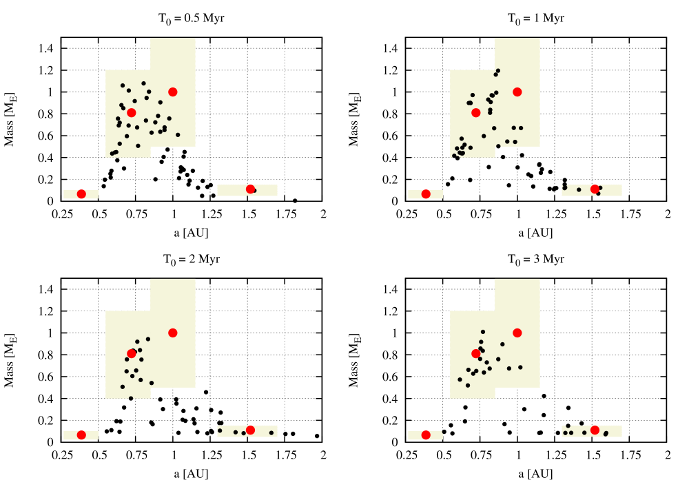
Figure 8: The final mass of the terrestrial planets versus their semi-major axis. The text above the panels indicates the time at which Jupiter and Saturn had formed and migrated into the inner solar system. Beige regions indicate the range of our terrestrial planet analogues. Oligarchic initial conditions with a tack at 1.5 AU.

In this subsection we report the results of Grand Tack simulations with the oligarchic initial conditions. Since we do not expect substantial differences between this model and the equal mass embryo one of Jacobson & Morbidelli (2014), we shall only report on the overall results.

Disc age [Myr]	$\langle n\rangle$	$\langle S_{c}\rangle$	$\langle$ AMD $\rangle$	$\langle S_{H}\rangle$
0.5	3.8 $\pm$ 0.7	133 $\pm$ 26	0.32 $\pm$ 0.33 (0.18)	26 $\pm$ 9
1	3.7 $\pm$ 0.7	120 $\pm$ 28	0.23 $\pm$ 0.17 (0.18)	29 $\pm$ 6
2	3.2 $\pm$ 0.6	127 $\pm$ 71	1.73 $\pm$ 2.64 (0.47)	38 $\pm$ 9
3	2.6 $\pm$ 0.6	110 $\pm$ 64	7.1 $\pm$ 5.3 (4.3)	52 $\pm$ 13

Table 3: Same as Table 2 for the oligarchic initial conditions and a tack at 1.5 AU.

Figures 8 and 9 are the oligarchic equivalents of Figs. 4 and 5. It appears that the correspondence with the real terrestrial system worsens as the time of the onset of migration increases. In the second figure the red dots are for the simulations where the disc age (time of the onset of migration) is 0.5 Myr. Orange dots are for a disc age of 1 Myr, green for 2 Myr and blue for 3 Myr. There are a few visible trends. First, the final AMD value tends to increase with increasing disc age. This is unsurprising because the total mass in planetesimals decreases as the disc ages, so there is less mass to exert dynamical friction on the forming planets. Half of all systems are within the AMD-$S_{c}$ boundaries in the bottom panel, but only 11% in the $S_{H}-S_{m}$ plot at the top, implying only 5% fall into both regions simultaneously, lower than in the equal mass embryo case. The equal mass simulations have nearly uniform spacing anywhere from 20 to over 50 Hill radii. Systems with older disc ages are more widely spaced, while systems with younger disc ages – and therefore lower embryo seed masses and more mass in planetesimals – tend to be compact, with a typical spacing of 20 Hill radii, reminiscent of extrasolar systems (Fang & Margot, 2013). The older systems also tend to have fewer planets, and these planets all appear to be of similar, sub-Venus masses because we observe a trend of a decreasing number of planets with older disc ages. The mean number of planets as a function of disc age are listed in Table 3.

Visually the results from the oligarchic model appear to be different from the equal mass embryo setup, but statistically the models are nearly identical (see Table 3). We report no Mercury analogues, a probability of $32\%\pm 3\%$ for Venus analogues, $10\%\pm 5\%$ for Earth analogues and $9\%\pm 5\%$ for Mars analogues. The location and mass of the most massive planet is $\langle a_{h}\rangle=0.782\,{\rm AU}\pm 0.089\,{\rm AU}$ and $\langle m_{h}\rangle=0.805M_{\oplus}\pm 0.160M_{\oplus}$, on the low side for both quantities. Once again the semi-major axis of the most massive planet is statistically inconsistent with the Earth’s. In addition, unlike the equal mass embryo case, we did not change the disc mass from one set of of simulations to the next, which could account for the lower mass of the most massive planet.

We point out that we only tested the oligarchic initial conditions for disc mass with a a surface density of $\Sigma_{0}=7$ g cm^-2 at 1 AU. It is possible that a higher initial surface density would lead to higher planetary masses at the end of the simulations. That said, it is unclear whether a higher surface density would increase the typical spacing between the planets, because of the weak dependence of the Hill radius on the mass.

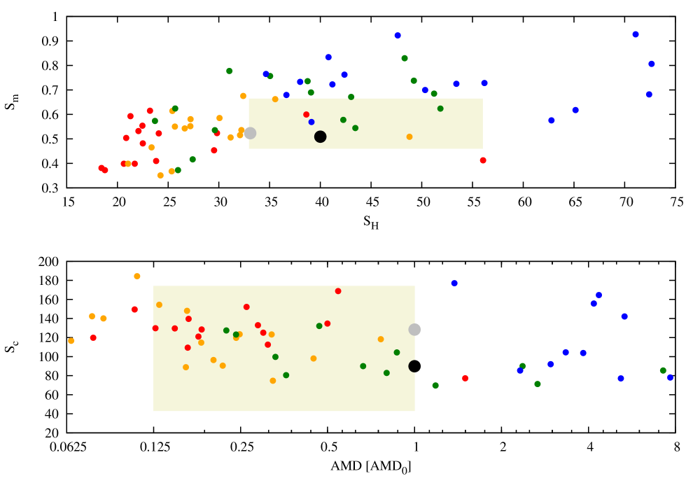
Figure 9: Top panel: Scatter plot of the spacing parameter $S_{H}$ vs the mass parameter $S_{m}$. Red symbols correspond to simulations with a disc age of 0.5 Myr, orange to initial disc age of 1 Myr, green dots have an initial disc age of 2 Myr and blue ones 3 Myr. Bottom: Scatter plot of concentration parameter $S_{c}$ vs normalised AMD. Oligarchic with tack at 1.5 AU.

When investigating the timing of the Moon-forming impact, we arrive at a time of 100 Myr, but once again the range is large, from 20 Myr to 120 Myr. The nominal value is a little later than favoured by the geochronology (Kleine et al., 2005; Touboul et al., 2007) or the plutogenic-xenon arguments of Avice & Marty (2014). In any case, the mass left in planetesimals after 150 Myr of simulation is 0.045 $M_{\oplus}\pm 0.029\,M_{\oplus}$, comparable to the equal mass embryo case. Both the timing of the Moon-forming impact and remnant mass are statistically the same as for the equal mass embryo case. Lastly, the growth of Mars proceeds similarly to that depicted in Fig. 7. In summary, both the oligarchic model and the equal mass embryo model are statistically identical within error margins, and we cannot favour one over the other. Further study is needed to distinguish the two.

7 Results: Tack at 2 AU

The simulations with a tack at 2 AU were performed to determine whether a more distant tack location would result in the Earth analogue being generally more massive than the Venus analogue and whether it improves the overall fit of the model with the current architecture of the terrestrial planets. Since much of the underlying dynamics are the same, we shall only report the highlights.

7.1 Equal mass embryos

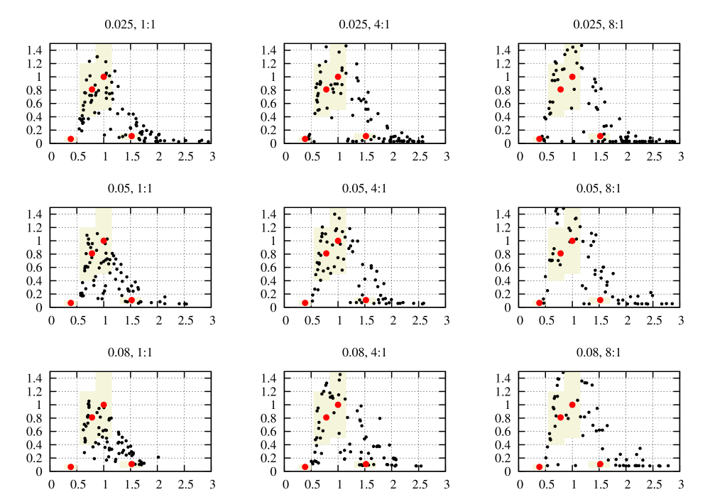
Figure 10: The final mass of the terrestrial planets versus their semi-major axis. The text above the panels indicates the embryo mass in Earth masses and the ratio of the total embryo to planetesimal mass. Beige regions indicate the range of our terrestrial planet analogues. Equal-mass embryo initial conditions with a tack at 2 AU.

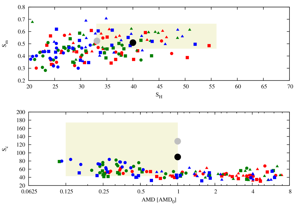
Figure 11: Top panel: Scatter plot of the spacing parameter $S_{H}$ vs the mass parameter $S_{m}$. Red symbols correspond to simulations with an initial embryo mass of 0.025$M_{\oplus}$, green to initial embryo mass of 0.05$M_{\oplus}$ and blue to initial embryo mass of 0.08$M_{\oplus}$. Bullets are for simulations with a total embryo to planetesimal mass ratio of 1:1, squares are for a 4:1 mass ratio and triangles for an 8:1 mass ratio. Bottom: Scatter plot of concentration parameter $S_{c}$ vs normalised AMD. Equal-mass embryo conditions with a tack at 2 AU.

Figure 10 is a scatter plot of the final semi-major axis and masses of the planets produced in our simulations. The wider, more massive disc will naturally produce more massive planets over a wider range of heliocentric distances, and the plot should be compared with Fig. 4. There are two visual differences between the two sets of outcomes. First, the peak of the distribution is now farther out than with a tack at 1.5 AU. Indeed, the mean semi-major axis of the most massive planet is at $\langle a_{h}\rangle=0.91\,{\rm AU}\pm 0.19\,{\rm AU}$, much closer to the current position of Earth than with a tack at 1.5 AU. The most massive planet now has a mean mass of $\langle m_{h}\rangle=1.15M_{\oplus}\pm 0.26M_{\oplus}$, which is more massive than Earth but well within error margins. This increased mass is most likely caused by the accretion annulus being wider, having been truncated at 1.25 AU rather than at 1 AU. The outward tail is also caused by the same effect. We explore whether this also implies that a tack at 2 AU produces a better overall outcome.

First, we report that the average probability of producing a Venus analogue is $17\%\pm 4\%$, an Earth analogue of $13\%\pm 5\%$ and a Mars analogue of $5\%\pm 3\%$. We also produce some Mercury analogues ($0.55\%\pm 0.83\%$). Overall, the production of Venus and Earth analogues is similar, while the production of Venus analogues was more than twice as high as Earth analogues when the tack occurred at 1.5 AU. The production of Mars analogues is low, at the threshold of acceptability, caused by the fact that we generally create more massive planets near Mars’ current position than with a tack at 1.5 AU.

In comparison to the equal mass embryo simulations with a tack at 1.5 AU the planetary systems generated here have more planets on average. This is especially true for the cases with embryos of 0.025 $M_{\oplus}$ and a high mass in planetesimals. We list the number of planets and the standard deviation in Table 4.

Embryo mass [$M_{\oplus}$]	$\langle n\rangle$	$\langle S_{c}\rangle$	$\langle$ AMD $\rangle$	$\langle S_{H}\rangle$
0.025	5.4 $\pm$ 1.5	46 $\pm$ 8	3.2 $\pm$ 2.8 (2.6)	33 $\pm$ 8
0.05	4.5 $\pm$ 1.0	53 $\pm$ 13	2.4 $\pm$ 3.9 (0.93)	33 $\pm$ 8
0.08	4.4 $\pm$ 1.0	52 $\pm$ 15	2.1 $\pm$ 3.1 (0.74)	32 $\pm$ 8
$M_{\rm emb}:M_{\rm pl}$	$\langle n\rangle$	$\langle S_{c}\rangle$	$\langle$ AMD $\rangle$	$\langle S_{H}\rangle$
1:1	5.0 $\pm$ 1.0	61 $\pm$ 13	1.0 $\pm$ 1.4 (0.36)	28 $\pm$ 7
4:1	4.9 $\pm$ 1.4	45 $\pm$ 9	2.6 $\pm$ 3.3 (1.1)	34 $\pm$ 8
8:1	4.5 $\pm$ 1.4	45 $\pm$ 9	4.1 $\pm$ 4.0 (3.1)	36 $\pm$ 7

Table 4: Same as Table 2 for the equal mass embryos initial conditions and a tack at 2 AU.

In Fig. 11 we once again plot the spacing parameter $S_{H}$ vs mass parameter $S_{m}$ in the top panel and concentration parameter $S_{c}$ vs normalised AMD in the bottom panel. A similar trend of decreasing $S_{c}$ with increasing AMD is visible, but not as pronounced. What is clear is that all of the systems have a concentration lower than or equal to that of the current terrestrial planets; none of them are higher (bottom panel). Since most systems have a spacing that is more compact than the current terrestrial planets (top panel), the lower concentration implies a lower variation in mass between the planets, which is generally what is observed in Fig. 10. Things take a turn for the worse when we try to match the ranges of $S_{c}$, $S_{m}$, $S_{H}$ and the AMD simultaneously. We find that only 3/144 cases do so, which is much lower than the 5% threshold we have adopted, and much lower than the 10% reported earlier when the tack was at 1.5 AU. This low probability argues against a tack location at 2 AU being suitable to reproduce the current architecture of the terrestrial planets with the equal mass embryo initial conditions, despite the visual accuracy of fit. We generally find that $S_{c}$ is low while $S_{H}$ and the AMD are comparable to the case with a tack at 1.5 AU, suggesting that the mass distribution is narrower and the mass variations between planets are less extreme. Most of the concentration values are low but within the acceptable range.

The last two issues are the timing of the Moon-forming impact, which is at 60 Myr but with the same range (30 Myr to 120 Myr) as reported earlier, and a leftover planetesimal mass of $0.053M_{\oplus}\pm 0.04M_{\oplus}$, once again on the high end but in agreement with simulations having a tack at 1.5 AU. The simulations with an initial 1:1 ratio have a typical final mass of 0.1 $M_{\oplus}$ while the 8:1 simulations typically have 0.02 $M_{\oplus}$. The decay follows a stretched exponential with best fits $\beta=0.44\pm 0.03$ and $\beta\log\tau=0.52\pm 0.05$, which results in a slower decay than with a tack at 1.5 AU and explains the higher leftover mass.

7.2 Oligarchic embryos

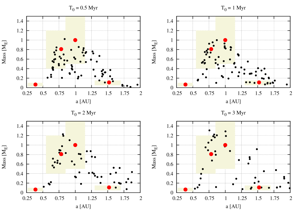
Figure 12: The final mass of the terrestrial planets versus their semi-major axis. The text above the panels indicates the time at which Jupiter and Saturn had formed and migrated into the inner solar system. Beige regions indicate the range of our terrestrial planet analogues. Oligarchic initial conditions with a tack at 2 AU.

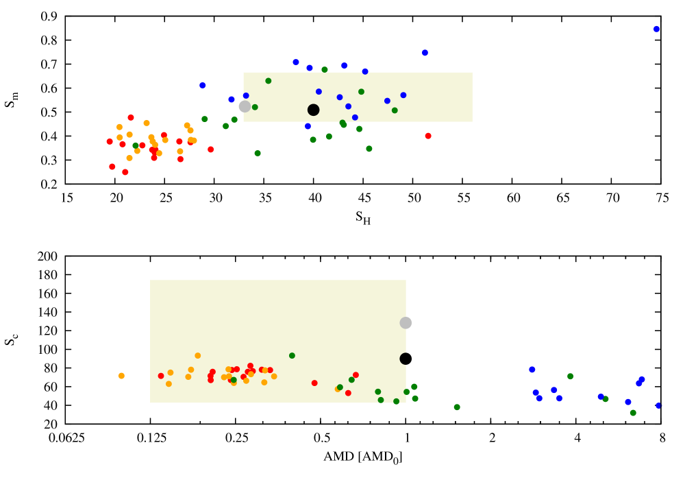
Figure 13: Top panel: Scatter plot of the spacing parameter $S_{H}$ vs the mass parameter $S_{m}$. Red symbols correspond to simulations with a disc age of 0.5 Myr, orange to initial disc age of 1 Myr, green dots have an initial disc age of 2 Myr and blue ones 3 Myr. Bottom: Scatter plot of concentration parameter $S_{c}$ vs normalised AMD. Oligarchic with tack at 2 AU.

In the previous subsection we investigated whether or not a tack location at 2 AU would yield a better outcome for the overall architecture of the terrestrial planets than a tack at 1.5 AU in the case of equal mass embryo initial conditions. We concluded that it appears to be difficult for this combination of tack location and initial conditions to simultaneously reproduce the combined spacing, concentration, mass distribution and AMD of the terrestrial planets, despite generating more Earth analogues and the heaviest planet being closer to Earth’s current location. It is now worth investigating whether the oligarchic system fares any better.

Figures 12 and 13 depict the relation between mass and semi-major axis, and spacing, concentration, mass and AMD distributions as usual. Once again we see a broader semi-major axis-mass distribution and an overall closer spacing and lower concentration. The concentration is, however, generally a little higher than in the equal mass embryo case. Indeed, we find that 10% of the outcomes fall within both beige regions simultaneously, higher than for the equal mass embryo case and comparable to the simulations with a tack at 1.5 AU. The production of terrestrial planet analogues is similar to the equal mass embryo case above so that we tend to produce more planets on average than with a tack at 1.5 AU, but somewhat fewer than the equal mass embryo case with a tack at 2 AU. The final results are listed in Table 5.

Similarly to the equal mass embryo case with a tack at 2 AU we produce Venus analogues $20\%\pm 3\%$ of the time, Earth analogues $13\%\pm 3\%$ of the time and Mars analogues with a probability of $6\%\pm 3\%$. The wider mass annulus also results in the heaviest planet having a mean semi-major axis of $\langle a_{h}\rangle=0.96\,{\rm AU}\pm 0.18\,{\rm AU}$, but its mean mass remains a little low at $\langle m_{h}\rangle=0.88M_{\oplus}\pm 0.18M_{\oplus}$, probably because we did not enhance the disc mass per set of simulations as we did for the equal mass embryo case. Once again the concentration value is low and we see $S_{H}\sim 25$ Hill radii for early disc ages and an increase in the AMD with disc age.

The Moon-forming impact occurs at 90 Myr, ranging from 30 Myr to 120 Myr depending on the amount of late accretion. The mass in leftover planetesimals is comparable to earlier simulations at $0.054M_{\oplus}\pm 0.038M_{\oplus}$.

Disc age [Myr]	$\langle n\rangle$	$\langle S_{c}\rangle$	$\langle$ AMD $\rangle$	$\langle S_{H}\rangle$
0.5	4.8 $\pm$ 0.8	73 $\pm$ 7	0.31 $\pm$ 0.14 (0.27)	25 $\pm$ 7
1	4.9 $\pm$ 0.6	72 $\pm$ 8	0.24 $\pm$ 0.11 (0.24)	24 $\pm$ 3
2	3.9 $\pm$ 0.8	53 $\pm$ 16	2.9 $\pm$ 3.6 (1.0)	38 $\pm$ 7
3	3.6 $\pm$ 0.7	48 $\pm$ 13	9.7 $\pm$ 8.8 (6.7)	43 $\pm$ 10

Table 5: Same as Table 2 for the oligarchic initial conditions and a tack at 2 AU.

7.3 Summary

The summary of our results is displayed in Table 6. The criteria we consider important are whether the model can produce Mars with a probability higher than 5%, whether the architecture of the system in terms of spacing, concentration, mass and AMD is consistent with the current planets, and whether the mass and semi-major axis of the heaviest planet are consistent with those of Earth. The Moon-forming impact is a less stringent criterion because of the inherent uncertainty in the late-accreted mass and the wide range of ages that appear as a result. All that matters is that it is within the error bars of the reported hafnium-tungsten ages, which it is, but it does not provide any further constraints on the model.

It appears that most initial conditions work to some extent. A tack at 2 AU is able to place the most massive planet near Earth’s current location and thus being the only model to satisfy the semi-major axis constraint of the heaviest planet. This statistically rules out a tack at 1.5 AU with the constraints that we impose and the disc parameters and migration prescription that we used. However, the equal mass embryo case with a tack at 2 AU is problematic because of its low ability to reproduce the spacing, concentration, mass and AMD ranges simultaneously. We are confident this low probability is inherent in the model and not caused by sampling and therefore we also rule it out. This leaves us with the oligarchic model with a tack at 2 AU. The remnant mass in planetesimals is an obvious concern, but the somewhat low mass of the most massive planet when the tack occurred at 2 AU cannot be statistically rejected. The disc age in the oligarchic model that best matches all constraints is 2 Myr, which is a typical time range to form the gas giants.

Type	Tack [AU]	Mars	Architecture	$\langle a_{h}\rangle$	$\langle m_{h}\rangle$	$t_{\rm Moon}$	Mass left [$M_{\oplus}$]
Equal mass	1.5 AU	✓	✓	✗	✓	✓	0.05$\pm$0.03
Equal mass	2 AU	✓	✗	✓	✓	✓	0.05$\pm$0.04
Oligarchic	1.5 AU	✓	✓	✗	✓	✓	0.05$\pm$0.03
Oligarchic	2 AU	✓	✓	✓	✓	✓	0.05$\pm$0.04

Table 6: Summary of the results of the different sets of simulations. It is clear that a tack location of 1.5 AU has difficulty reproducing the current Solar System; a tack at 2 AU is preferred.

We point out that the above conclusions, drawn from Table 6 are valid for the disc model that we have employed. We return to its implications in the next section. One thing we have not mentioned thus far is the total mass of material we emplace in the asteroid belt. This matter is discussed in detail in the next section.

8 Discussion

In this study we ran a high number of terrestrial planet simulations in the framework of the Grand Tack model with a range of initial conditions and two different tack locations. In the previous subsection we concluded that, despite using a different model for the protoplanetary disc, the inclusion of type 1 migration and a realistic mass-radius relationship, the outcomes of our simulations are broadly similar, though each setup has its own unique pros and cons.

We have decided to use a different disc model than the traditional setup of Walsh et al. (2011) and we have outlined our reasons for doing so. We find that a tack at 1.5 AU leaves too much mass near Venus’ location. We attribute this to a combination of type 1 migration and inward shepherding by Jupiter, which decreases the semi-major axis of material down to below 1 AU but increases the eccentricity, so that further inward migration will ensue. This raises the question as to how sensitive our results are to the choice of disc model. This can only be answered by running more simulations with varying disc parameters, which is beyond the scope of the current study. We have used a relatively hot and puffy disc, with a scale height that is higher than traditional values (Hayashi, 1981; Tanaka et al., 2002; Tanaka & Ward, 2004) caused by viscous heating in the inner disc. This higher scale height causes slower embryo migration. Thus, making use of a colder, thinner disc would likely have exacerbated the overproduction of Venus analogues with a tack at 1.5 AU. One way to mitigate this problem is to use a much lower surface density, as was done by Walsh et al. (2011) and Jacobson & Morbidelli (2014) but their values seem artificial. A much lower surface density would decrease the migration rate of Jupiter and Saturn, and even though their migration rate does not appear to affect the final orbital architecture of the terrestrial system (Walsh et al., 2011), it does increase the difficulty for these planets to reach their final positions beyond 5 AU (D’Angelo & Marzari, 2012). Thus, even when using a colder, less massive disc, we still expect to see an overproduction of Venus analogues when the tack occurred near 1.5 AU.

A second topic concerns the timing of the Moon-forming impact. We generally find agreement between our typical time of 60-90 Myr and geochronology. However, our uncertainties are typically 30 Myr or longer, suggesting the GI occurred anywhere from 30 Myr to 120 Myr, which is what we have claimed in the previous sections. It is debatable whether this range implies anything meaningful. It is consistent with the value 95$\pm$32 Myr reported in Jacobson et al. (2014), even though they ran their simulations for a little longer and used a much lower amount of late accreted mass. In summary, we do not think that our simulations, nor those of Jacobson et al. (2014), can say anything meaningful about the timing of the GI beyond what is known from geochronology.

Another issue that requires discussion is the mass left over in planetesimals after planet formation. This is typically 0.05 $M_{\oplus}$ but can be as high as 0.1 $M_{\oplus}$. This leftover mass has implications for the cratering rates on Noachian Mars and the Pre-Nectarian Moon. The most efficient way to eliminate this material is through collision with the terrestrial planets. Ejection by the giant planets or collisions with the Sun is much more difficult. Preliminary simulations of this population of planetesimals indicate it decays slowly, following a stretched exponential with stretching parameter $\beta\sim 0.83$ and e-folding time $\tau\sim 85$ Myr. A slow decay is preferred by lunar cratering records (Werner et al., 2014), but a slower decay is necessary so as not to have late melting of the crust of the planets (Abramov et al., 2013); Abramov & Mojzsis (2016).

One solution may be for these planetesimals to grind themselves to dust and subsequently be lost through Poynting-Robertson drag or radiation pressure. The difficulty with this idea is that the high ratio of highly siderophile elements in the Earth and Moon suggest that the Late Veneer impactors were large (around 2000 km) (Bottke et al., 2010). If these impactors were large there is no reason to believe the impactors after the Late Veneer were substantially smaller. A simple argument is that Ceres is the only 1000 km body in the asteroid belt, and with a typical implantation probability of 0.1% (Walsh et al., 2011), there should have been at least 1000 Ceres-sized bodies. With of the order of 5% of the total mass remaining after 150 Myr we have 50 Ceres-sized bodies still present, with perhaps ten bodies the size of 4000 km. Since it was probable that the size distribution of the remnant planetesimals was shallow (Bottke et al., 2010), most of the mass is in the large bodies, and thus we consider it very unlikely that this mass was ground down by collisional erosion.

A quick estimate of the collisional time scale can be made with an $n\sigma vt=1$ argument, where $n$ is the number density of planetesimals, $v$ is their typical encounter velocity, and $\sigma=\pi r^{2}$ is their collisional cross section. The number density $n=M/(2\pi^{2}a^{2}m\Delta a\sin i)$, where $M$ is the total mass of remnant planetesimals, $\Delta a$ is the width of the annulus in which the planetesimals are situated and $m$ is their individual mass. We then have

$$\frac{3Mvt}{8\pi^{2}a^{2}\Delta a\sin i\rho r}=1.$$ (16)

From our simulations we find that the typical semi-major axis of these planetesimals is 1.5 AU and $\Delta a\sim 0.5$ AU, $i\sim 20^{\circ}$ and using a planetesimal density of $\rho=3000$ kg m^-3 and encounter velocity $v\sim ev_{K}\sim 12$ km s^-1 we have for a planetesimal of radius 500 km that $t>1$ Gyr. This is longer than the estimate of 56 Myr of Raymond et al. (2013) because they consider a smaller annulus and a planar problem. Thus for large planetesimals, collisional grinding is most likely unimportant, though future studies need to verify or deny this claim. In any case, the amount of leftover material warrants a separate investigation, in particular if the size distribution is shallow and most mass is in large planetesimals. Its results will be discussed in a companion paper.

Another topic that was not discussed in the previous sections was the amount of mass that is placed in the asteroid belt. With our definition of the asteroid belt region (perihelion $q>1.6$ AU and aphelion $Q<4.5$ AU), we find that simulations with a tack at 1.5 AU place roughly 0.6% of material in the asteroid belt, while this increases to 0.9% when the tack is at 2 AU, comparable to but slightly in excess of the percentage reported by Walsh et al. (2011). The main reason our simulations with a tack at 1.5 AU have a higher amount of mass in the asteroid belt than theirs is due to the stronger gas drag acting on planetesimals in the beginning of the simulations because the surface density of our disc is higher than theirs. The higher value with the tack at 2 AU is clearly a result of weaker sculpting of the disc by Jupiter. All of these simulations leave us with an asteroid belt whose mass is at least an order of magnitude higher than the current value, with the caveat that we only used planetesimals with a size of 50 km for the purpose of the gas drag. Larger planetesimals would have reduced the remnant mass in the asteroid belt while a smaller size would have increased it (Matsumura et al., 2016). It has been suggested that chaotic diffusion over 4 Gyr and giant planet evolution deplete the belt by approximately 75% of its mass, but then the remaining amount of mass is still inconsistent with what is observed today (Minton & Malhotra, 2010). Then again, our simulations do not take collisional erosion into account, which could erode the belt even further (Bottke et al., 2005).

A final topic that requires discussion is the total number of planets. When taking each set of initial conditions as a whole, the total number of planets is 4.4 $\pm$ 1.3 for the equal mass embryo case with a tack at 1.5 AU, 3.3 $\pm$ 0.8 for the oligarchic case with a tack at 1.5 AU, 4.8 $\pm$ 1.3 for the equal mass embryo case with a tack at 2 AU and 4.3 $\pm$ 0.9 for the oligarchic case with a tack at 2 AU. All of these are consistent with four terrestrial planets at the end. Yet, most of our simulations do not produce a Mercury analogue. This is a result of the initial conditions that we have employed, and it is noteworthy that the formation of Mercury has been mostly ignored in earlier works (Walsh et al., 2011; O’Brien et al., 2014; Jacobson et al., 2014; Jacobson & Morbidelli, 2014; Jacobson & Walsh, 2015). If we are to ignore it too, then the total number of planets we must produce is three. All models as a whole are statistically consistent with three terrestrial planets, though some subsets within the four models are not. Since the formation and evolution of Mercury are currently unknown, further study is needed to rule out whether the oligarchic model with a tack at 2 AU can be made consistent with the current inner solar system. It is possible that by the end of our simulations the final system is not stable in the long-term and a very late collision could remove another planet. This is inconsistent with the historical evolution of the Solar System so we have to take the number of planets at the end of the simulations as final.

9 Conclusions

We have investigated the dynamical formation of the terrestrial planets in the framework of the Grand Tack scenario. It has been claimed that the Grand Tack reproduces several observed features of the inner Solar System that previous models failed to do, such as the low mass of Mars and the compositional gradient in the asteroid belt. We examined this scenario in more detail here but applied a different disc profile, a realistic mass-radius relationship, and took into account type 1 migration. We have stated our reasons for doing so in Section 2, and performed sensitivity tests to determine whether any of these differences matter. The answer appears to be ’yes’: with the initial conditions and disc and migration model that we employed we statistically ruled out a tack at 1.5 AU because we produced an excess of Venus analogues and a deficit of Earth analogues. We attribute this excess of Venus analogues to our disc model because it has a higher surface density than the one of Walsh et al. (2011). Additionally, with more than 95% confidence, the semi-major axis of the most massive planet is inconsistent with Earth’s location, while upon a visual inspection of their results the same is not true in the simulations of Jacobson & Morbidelli (2014). Thus the inclusion of type 1 migration, and a much higher initial disc surface density, together with smaller radii of the planets, serve to shift the mass distribution closer to the Sun. This calls for a more distant tack location. We find that the model that best matches the current architecture of the terrestrial planets has a tack at 2 AU and oligarchic initial conditions.

We thank Kevin Walsh for making available to us his version of SyMBA that incorporates the migration of the gas giants and the gas profile, Hal Levison for indicating we should include a realistic mass-radius relationship, and an anonymous reviewer for constructive comments. RB is grateful for financial support from the Astrobiology Center Project of the National Institutes of Natural Sciences (NINS) grant number AB271017 and to the Daiwa Anglo-Japanese Foundation for a Small Grant. RB and SJM acknowledge the John Templeton Foundation - Ffame Origins program in the support of CRiO. SJM is grateful for support by the NASA Exobiology Program (NNH14ZDA001N-EXO). SCW is supported by the Research Council of Norway (235058/F20 CRATER CLOCK) and through the Centres of Excellence funding scheme, project number 223272 (CEED). Numerical simulations were in part carried out on the PC cluster at the Center for Computational Astrophysics, National Astronomical Observatory of Japan.

Abramov, O., and Mojzsis, S.J. (2016). Earth and Planetary Science Letters. -in press-
Levison, H. F., Kretke, K. A., Walsh, K. J. & Bottke, W. F.  2015, PNAS 112, 14181
Safronov, V. S. 1969, Evolution of the protoplanetary cloud and formation of the earth and planets. Translated from Russian (1969). Jerusalem (Israel): Israel Program for Scientific Translations, Keter Publishing House, 212 p. 1

References

- Abramov et al. (2013) Abramov, O., Kring, D. A., & Mojzsis, S. J. 2013, Chemie der Erde / Geochemistry, 73, 227
- Albarède et al. (2013) Albarede, F., Ballhaus, C., Blichert-Toft, J., et al. 2013, Icarus, 222, 44
- D’Angelo & Marzari (2012) D’Angelo, G., & Marzari, F. 2012, ApJ, 757, 50
- Avice & Marty (2014) Avice, G., & Marty, B. 2014, Royal Society of London Philosophical Transactions Series A, 372, 30260
- Bitsch et al. (2015) Bitsch, B., Johansen, A., Lambrechts, M., & Morbidelli, A. 2015, A&A, 575, A28
- Bottke et al. (2005) Bottke, W. F., Durda, D. D., Nesvorný, D., et al. 2005, Icarus, 179, 63
- Bottke et al. (2010) Bottke, W. F., Walker, R. J., Day, J. M. D., Nesvorny, D., & Elkins-Tanton, L. 2010, Science, 330, 1527
- Bottke et al. (2015) Bottke, W. F.,Vokrouhlický, D., Marchi, S., et al. 2015, Science, 348, 321
- Brasser et al. (2007) Brasser, R., Duncan, M. J., & Levison, H. F. 2007, Icarus, 191, 413
- Brasser et al. (2013) Brasser, R., Walsh, K. J., & Nesvorný, D. 2013, MNRAS, 433, 3417
- Carlson et al. (2015) Carlson, R. W., Borg, L. E., Gaffney, A. M. & Boyet, M. 2015, Philosophical Transactions of the Royal Society 372, 1
- Chambers (2001) Chambers, J. E. 2001, Icarus, 152, 205
- Chambers (2006) Chambers, J. 2006, Icarus, 180, 496
- Cresswell & Nelson (2008) Cresswell, P., & Nelson, R. P. 2008, A&A, 482, 677
- Dauphas & Pourmand (2011) Dauphas, N., & Pourmand, A. 2011, Nature, 473, 489
- Debaille et al. (2007) Debaille, V., Brandon, A. D., Yin, Q. Z., & Jacobsen, B. 2007, Nature, 450, 525
- DeMeo & Carry (2014) DeMeo, F. E., & Carry, B. 2014, Nature, 505, 629
- Duncan et al. (1998) Duncan, M. J., Levison, H. F., & Lee, M. H. 1998, AJ, 116, 2067
- Elkins-Tanton et al. (2005) Elkins-Tanton, L. T., Hess, P. C.,& Parmentier, E. M. 2005, Journal of Geophysical Research (Planets), 110, E12S01
- Fang & Margot (2013) Fang, J., & Margot, J.-L. 2013, ApJ, 767, 115
- Guillot & Hueso (2006) Guillot, T., & Hueso, R. 2006, MNRAS, 367, L47
- Halliday (2008) Halliday, A. N. 2008, Royal Society of London Philosophical Transactions Series A, 366, 4163
- Hansen (2009) Hansen, B. M. S. 2009, ApJ, 703, 1131
- Hartmann et al. (1998) Hartmann, L., Calvet, N., Gullbring, E., & D’Alessio, P. 1998, ApJ, 495, 385
- Hayashi (1981) Hayashi, C. 1981, Progress of Theoretical Physics Supplement, 70, 35
- Hueso & Guillot (2005) Hueso, R., & Guillot, T. 2005, A&A, 442, 703
- Humayun et al. (2013) Humayun, M., Nemchin, A., Zanda, B., et al. 2013, Nature, 503, 513
- Izidoro et al. (2014) Izidoro, A., Haghighipour, N., Winter, O. C., & Tsuchida, M. 2014, ApJ, 782, 31
- Izidoro et al. (2015) Izidoro, A., Raymond, S. N., Morbidelli, A., & Winter, O. C. 2015, MNRAS, 453, 3619
- Jacobson & Morbidelli (2014) Jacobson, S. A., & Morbidelli, A. 2014, Royal Society of London Philosophical Transactions Series A, 372, 0174
- Jacobson et al. (2014) Jacobson, S. A.,Morbidelli, A., Raymond, S. N., et al. 2014, Nature, 508, 84
- Jacobson & Walsh (2015) Jacobson, S. A., & Walsh, K. J. 2015, Earth and Terrestrial Planet Formation, in The Early Earth: Accretion and Differentiation (eds J. Badro and M. Walter), John Wiley & Sons, Inc, Hoboken, NJ.
- Kinoshita et al. (1991) Kinoshita, H., Yoshida, H., & Nakai, H. 1991, Celest. Mech. Dyn. Astron., 50, 59
- Kleine et al. (2005) Kleine, T., Palme, H., Mezger, K., & Halliday, A. N. 2005, Science, 310, 1671
- Kokubo & Ida (1996) Kokubo, E., & Ida, S. 1996, Icarus, 123, 180
- Kokubo & Ida (1998) Kokubo, E., & Ida, S. 1998, Icarus, 131, 171
- Laskar (2008) Laskar, J. 2008, Icarus, 196, 1
- Lin & Papaloizou (1986) Lin, D. N. C., & Papaloizou, J. 1986, ApJ, 309, 846
- Masset & Snellgrove (2001) Masset, F., & Snellgrove, M. 2001, MNRAS, 320, L55
- Masset & Casoli (2009) Masset, F. S., & Casoli, J. 2009, ApJ, 703, 857
- Marty (2012) Marty, B. 2012, Earth and Planetary Science Letters, 313, 56
-
Matsumura et al. (2016)
Matsumura, S., Brasser, R. & Ida, S. 2016, ApJ, in press
- Minton & Malhotra (2010) Minton, D. A., & Malhotra, R. 2010, Icarus, 207, 744
- Morbidelli & Crida (2007) Morbidelli, A., & Crida, A. 2007, Icarus, 191, 158
- Morbidelli et al. (2007) Morbidelli, A., Tsiganis, K., Crida, A., Levison, H. F., & Gomes, R. 2007,AJ, 134, 1790
- Morbidelli et al. (2012) Morbidelli, A., Marchi, S., Bottke, W. F., & Kring, D. A. 2012, Earth and Planetary Science Letters, 355, 144
- Morbidelli et al. (2015) Morbidelli, A., Lambrechts, M., Jacobson, S., & Bitsch, B. 2015, Icarus, 258, 418
- Nimmo & Kleine (2007) Nimmo, F., & Kleine, T. 2007, Icarus, 191, 497
- O’Brien et al. (2006) O’Brien, D. P., Morbidelli, A., & Levison, H. F. 2006, Icarus, 184, 39
- O’Brien et al. (2014) O’Brien, D. P., Walsh, K. J., Morbidelli, A., Raymond, S. N., & Mandell, A. M. 2014, Icarus, 239, 74
- Ogihara & Ida (2009) Ogihara, M., & Ida, S. 2009, ApJ, 699, 824
- Paardekooper et al. (2011) Paardekooper, S.-J., Baruteau, C., & Kley, W. 2011, MNRAS, 410, 293
- Pierens & Nelson (2008) Pierens, A., & Nelson, R. P. 2008, A&A, 482, 333
- Pierens & Raymond (2011) Pierens, A., & Raymond, S. N. 2011, A&A, 533, A131
- Pierens et al. (2014) Pierens, A., Raymond, S. N., Nesvorny, D., & Morbidelli, A. 2014, ApJ, 795, L11
- Raymond et al. (2009) Raymond, S. N., O’Brien, D. P., Morbidelli, A., & Kaib, N. A. 2009, Icarus, 203, 644
- Raymond et al. (2013) Raymond, S. N.,Schlichting, H. E., Hersant, F., & Selsis, F. 2013, Icarus, 226, 671
- Rubie et al. (2015) Rubie, D. C., Jacobson, S. A., Morbidelli, A., et al. 2015, Icarus, 248, 89
- Seager et al. (2007) Seager, S., Kuchner, M., Hier-Majumder, C. A., & Militzer, B. 2007, ApJ, 669, 1279
- Tanaka et al. (2002) Tanaka, H., Takeuchi, T., & Ward, W. R. 2002, ApJ, 565, 1257
- Tanaka & Ward (2004) Tanaka, H., & Ward, W. R. 2004, ApJ, 602, 388
- Touboul et al. (2007) Touboul, M., Kleine, T., Bourdon, B., Palme, H., & Wieler, R. 2007, Nature, 450, 1206
- Touboul et al. (2009) Touboul, M., Kleine, T., Bourdon, B., Palme, H., & Wieler, R. 2009, Icarus, 199, 245
- Tsiganis (2015) Tsiganis, K. 2015, Nature528, 202
- Walker (2009) Walker, R. J. 2009, Chemie der Erde / Geochemistry, 69, 101
- Walsh et al. (2011) Walsh, K. J., Morbidelli, A., Raymond, S. N., O’Brien, D. P., & Mandell, A. M. 2011, Nature, 475, 206
- Warren & Wasson (1979) Warren, P. H., & Wasson, J. T. 1979, Reviews of Geophysics and Space Physics, 17, 73
- Werner et al. (2014) Werner, S. C., Ody, A., & Poulet, F. 2014, Science, 343, 1343
- Wetherill (1980) Wetherill, G. W. 1980, ARA&A, 18, 77
- Wetherill & Stewart (1989) Wetherill, G. W., & Stewart, G. R. 1989, Icarus, 77, 330
- Wisdom & Holman (1991) Wisdom, J., & Holman, M. 1991, AJ, 102, 1528
- Zhang & Zhou (2010) Zhang, H., & Zhou, J.-L. 2010, ApJ, 714, 532