Parameterizing Stellar Spectra Using Deep Neural Networks

Abstract

This work investigates the spectrum parameterization problem using deep neural networks (DNNs). The proposed scheme consists of the following procedures: first, the configuration of a DNN is initialized using a series of autoencoder neural networks; second, the DNN is fine-tuned using a gradient descent scheme; third, stellar parameters ($T_{\texttt{eff}}$, log$~{}g$, and [Fe/H]) are estimated using the obtained DNN. This scheme was evaluated on both real spectra from SDSS/SEGUE and synthetic spectra calculated from Kurucz’s new opacity distribution function models. Test consistencies between our estimates and those provided by the spectroscopic parameter pipeline of SDSS show that the mean absolute errors (MAEs) are 0.0048, 0.1477, and 0.1129 dex for log$~{}T_{\texttt{eff}}$, log$~{}g$, and [Fe/H] (64.85 K for $T_{\texttt{eff}}$), respectively. For the synthetic spectra, the MAE test accuracies are 0.0011, 0.0182, and 0.0112 dex for log$~{}T_{\texttt{eff}}$, log$~{}g$, and [Fe/H] (14.90 K for $T_{\texttt{eff}}$), respectively.

1 INTRODUCTION

Large-scale sky survey programs, such as the Sloan Digital Sky Survey (SDSS; York et al., 2000; Ahn et al., 2012), Large Sky Area Multi-Object Fiber Spectroscopic Telescope/Guoshoujing Telescope (LAMOST; Zhao et al., 2006; Cui et al., 2012), and Gaia-ESO Survey (Gilmore et al., 2012; Randich et al., 2013), are collecting and will obtain very large numbers of stellar spectra. This large amount of data necessitates a fully automated process to characterize the spectra, which will consequently enable the statistical exploration of atmospheric parameter-related properties in the spectra.

The present work studies the spectrum parameterization problem. A typical class of schemes are based on (feedforward) neural networks ((F)NNs: Willemsen et al., 2005; Giridhar et al., 2006; Re Fiorentin et al., 2007; Gray et al., 2009; Tan et al., 2013a). In these NNs, the information moves in only one direction, that is from the input nodes (neurons), through the hidden nodes, and to the output nodes (neurons). In atmospheric parameter estimation, the input nodes represent a stellar spectrum, and the output node(s) represent(s) the atmospheric parameter(s) to be estimated, e.g., $T_{\texttt{eff}}$, log $g$ and [Fe/H]. A NN is commonly obtained by a back-propagation (BP) algorithm (Rumelhart et al., 1986).

For example, Bailer-Jones (2000) investigated the estimation precision of stellar parameters $T_{\texttt{eff}}$, log$~{}g$, and [M/H] using a FNN network with two hidden layers on synthetic spectra with different resolutions and signal-to-noise ratios. Snider et al. (2001) explored the application of FNN with one and two hidden layers in the estimation of atmospheric parameters from medium-resolution spectra of F- and G-type stars. Manteiga et al. (2010) parameterized stellar spectra by extracting features based on Fourier analysis and wavelet decomposition, and constructing a mapping from a feature space to the parameter space by a FNN with one hidden layer. Li et al. (2014) investigated the atmospheric parameter estimation problem by detecting spectral features by LASSO first and subsequently estimating the atmospheric parameters using a FNN with one hidden layer.

This article investigates the spectrum parameterization problem using a deep NN (DNN). In application, a traditional NN usually has one or two hidden layers. By contrast, DNNs have two typical characteristics: 1) A DNN usually has more hidden layers, 2) Two procedures are needed in estimating a DNN: prelearning and fine-tuning. This scheme has been studied extensively in artificial intelligence and data mining, and shows excellent performance in many applications. This work investigated the application of this scheme in spectrum parameterization.

This paper is organized as follows. Section 2 introduces the NN, DNN, their learning algorithms, and the proposed stellar parameter estimation scheme. Section 3 reports some experimental evaluations on real and synthetic spectra. Finally, we summarize our work in Section 4.

2 Parameterizing stellar spectra using a DNN

2.1 A neural network (NN)

This work investigated a scheme to parameterize a stellar spectrum using a DNN. A NN consists of a series of neurons on multiple layers. Figure 1 is a diagram of a NN with $L$ layers. In this diagram, every circle with solid line represents a neuron, and a circle with a dashed line is a bias unit used in describing the relationships between neurons.

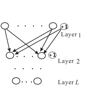
Figure 1: A diagram of a neural network.

In a NN, every neuron is a simple computational units and has an input and output, $z$ and $a$, respectively. For example, the $z^{(l)}_{k}$ and $a^{(l)}_{k}$ denote the input and output of the $k$-th neuron on the $l$-th layer, respectively, where $l=1,2,\cdots,L$; $k=1,\cdots,n_{l}$; and $n_{l}$ is the number of neurons on the $l$-th layer. The relationship between an input and output is usually described by an activation function $g(\dot{)}$:

$$a=g(z).$$ (1)

Two common choices for the activation function are a sigmoid function

$$g(z)=\frac{1}{1+e^{-z}}$$ (2)

and hyperbolic tangent function

$$g(z)=\frac{e^{z}-e^{-z}}{e^{z}+e^{-z}}.$$ (3)

The present work used the sigmoid function in equation (2).

A neuron receives signals from every neuron on the previous layer as the following:

$$z^{(l+1)}_{k}=\sum^{n_{l}}_{i=1}w^{(l)}_{ki}a^{(l)}_{i}+b^{(l)}_{k},$$ (4)

where $l=1,\cdots,L-1$, and $w^{(l)}_{ki}$ describe the relationship between the $k$th and the $i$th neurons on the $(l+1)$th and $l$th layers (this relationship is represented with a line between the two neurons in Fig. 1), respectively; $b^{(l)}_{k}$ is the bias associated with the $k$th neuron on the $(l+1)$th layer (represented with a line between the $k$th neuron and bias unit on the $(l+1)$th and $l$th layers, respectively), and $n_{l}$ is the number of neurons on the $l$th layer.

Generally, the first and last layers are called as input and output layers, respectively; the other layers are referred to as hidden layers. On the input layer, the output of a neuron is the same with its input

$$a^{(1)}_{k}=z^{(1)}_{k},k=1,\cdots,n_{1}.$$ (5)

The output of the last layer can be denoted as $\bm{a}^{(L)}$:

$$\bm{a}^{(L)}=(a^{(L)}_{1},\cdots,a^{(L)}_{n_{L}}).$$ (6)

Suppose $\bm{x}=(x_{1},\cdots,x_{n_{1}})^{T}$ is a representation of a signal (e.g., a stellar spectrum). If the $\bm{x}$ is an input into a NN in Figure 1:

$$\bm{z}^{(1)}=\bm{x},$$ (7)

an output $\bm{a}^{(L)}$ can be computed by this network (equations 4 and 1), where $\bm{z}^{(1)}=(z^{(1)}_{1},\cdots,z^{(1)}_{n_{1}})^{T}$. Therefore, a NN implements a non-linear mapping $h_{\bm{W},\bm{b}}(\cdot)$ from an input $\bm{x}=(x_{1},\cdots,x_{n_{1}})^{T}$ to an output $\bm{a}^{(L)}$:

$$\bm{a}^{(L)}=h_{\bm{W},\bm{b}}(\bm{x}),$$ (8)

where

$$\bm{b}=\{\bm{b}^{(l)}\}$$ (9)

is the set of biases,

$$\bm{W}=\{\bm{W}^{(l)},l=1,\cdots,L\}$$ (10)

the set of the weights of a NN in equation (4), $\bm{b}^{l}=\{b^{(l)}_{j},1\leq j\leq n_{l}\}$ and $\bm{W}^{(l)}=\{W^{(l)}_{ji}\}$.

To define a NN, besides $L$, $\bm{W}$ and $\bm{b}$, one more set of parameters exists:

$$(n_{1},n_{2},\cdots,n_{L})$$ (11)

2.2 A BP algorithm for obtaining a NN

Suppose that

$$S=\{(\bm{x},\bm{y})\}$$ (12)

is a training set for a NN, where $\bm{x}=(x_{1},\cdots,x_{n_{1}})^{T}$ can be a representation of a spectrum, and $\bm{y}$ is the expected output corresponding to $\bm{x}$. Section 3.1 discusses more about the training set.

In a NN, some parameters $\bm{W}$ and $\bm{b}$ can be given. These parameters can be obtained by minimizing an objective function, namely, $J$, in equation (13):

$$J(\bm{W},\bm{b})= \frac{1}{N}\sum_{\bm{x}\in S}(\frac{1}{2}\|h_{\bm{W},\bm{b}}(\bm{x})-\bm{y}\|^{2})$$ (13)

$$+\frac{\lambda}{2}\sum^{L-1}_{l=1}\sum^{n_{l}}_{i=1}\sum^{n_{l+1}}_{j=1}(w^{(l)}_{ji})^{2},$$

where $N$ is the number of samples in a training set $S$, and $\lambda\geq 0$ is a preset parameter. In literature, $\lambda$ is commonly referred to as a weight decay parameter.

In equation (13), the first term represents an empirical error evaluation between the actual and expected outputs of an autoencoder; this term also ensures a good reconstruction performance of the network. The second term, a regularization term of $w^{(l)}_{ji}$, is used to overcome possible overfitting to the training set by reducing the scheme’s complexity.

To obtain our NN from a training set, we initialize each parameter $w^{(l)}_{ij}$ and $b^{(l)}_{i}$ to a small random value near zero; subsequently, two parameters $\bm{W}$ and $\bm{b}$ are iteratively optimized using a gradient descent method based on the objective function $J$ in equation (13). This learning scheme is referred to as BP algorithm (Rumelhart et al., 1986; Andrew et al., 2010).

2.3 Self-Taught Learning to DNNs

In a BP algorithm, the parameters $\bm{W}$ and $\bm{b}$ are initialized with a small random value. However, the obtained results of BP algorithm is unsatisfactory when the number of layers of a NN is higher than 4. In this case, $\bm{b}=\{\bm{b}^{(l)}\}$ and $\bm{W}=\{\bm{W}^{(l)},l=1,\cdots,L\}$ can be initialized using autoencoder networks.

An autoencoder is a specific kind of NN with three characteristics:

1. [*]

2. Only one hidden layer exists. The number of neurons in this layer is referred to as $n_{2}^{ae}$.

3. The number of neurons in the output layer is equal to that in the input layer. The number of neurons in input layer is represented by $n_{1}^{ae}$.

4. The expected output of the NN is NN’s input.

Therefore, the parameters of an autoencoder are $\bm{b}^{ae}$, $\bm{W}^{ae}$, and $n^{ae}$, where $\bm{b}^{ae}=\{\bm{b}^{(1,ae)},\bm{b}^{(2,ae)}\}$ is a set of biases, $\bm{W}^{ae}=\{\bm{W}^{(1,ae)},\bm{W}^{(2,ae)}\}$ a set of weights between neurons on different layers, and $n^{ae}=(n_{1}^{ae},n_{2}^{ae})$ numbers of neurons on input layer and hidden layer.

Therefore, to obtain a DNN (Figure 1), the proposed learning scheme consists of the following processes:

1. [1)]

2. Initialization using autoencoders.  To initialize the parameters $\bm{W}^{(1)}$ and $\bm{b}^{(1)}$ in equations (10) and (9), an autoencoder with $(n_{1}^{ae},n_{2}^{ae})=(n_{1},n_{2})$ is established; $\bm{W}^{ae}=\{\bm{W}^{(1,ae)},\bm{W}^{(2,ae)}\}$ and $\bm{b}^{ae}=\{\bm{b}^{(1,ae)},\bm{b}^{(2,ae)}\}$ are obtained from a training set $S^{(1)}=\{(x,x),x\in S\}$ using the BP algorithm (section 2.2) and let $\bm{W}^{(1)}=\bm{W}^{(1,ae)}$ and $\bm{b}^{(1)}=\bm{b}^{(1,ae)}$, where $n_{1}$ and $n_{2}$ are defined in equation (11). To initialize $\bm{W}^{(l)}$ and $\bm{b}^{(l)}$, the training set $S$ is input into the DNN in Fig. 1 to produce the outputs $S^{(l)}$ from the $l$th layer of the DNN in Fig. 1; Subsequently, an autoencoder with $(n_{1}^{ae},n_{2}^{ae})=(n_{l},n_{l+1})$ is established, $\bm{W}^{ae}=\{\bm{W}^{(1,ae)},\bm{W}^{(2,ae)}\}$ and $\bm{b}^{ae}=\{\bm{b}^{(1,ae)},\bm{b}^{(2,ae)}\}$ are obtained from the training set $S^{(l)}$ using the BP algorithm (section 2.2), the computed $\bm{W}^{(1,ae)}$ and $\bm{b}^{(1,ae)}$ are the initializations of $\bm{W}^{(1)}$ and $\bm{b}^{(1)}$, respectively, where $l=2,\cdots,L$.

3. Fine-tuning.  From the initialized $\bm{W}$ and $\bm{b}$ from the autoencoders, these two parameters are optimized using a gradient descent method based on the objective function $J$ in equation (13) (this optimization procedure is the same with that in the BP algorithm: section 2.2, Andrew et al., 2010).

2.4 Spectrum parameterization and performance evaluation

This work parameterizes stellar spectra using a NN with six layers; its configurations of the DNN are $L=6$ and $(n_{1},\cdots,n_{6})=(3821,1000,500,100,30,1)$, where $n_{l}$ is the number of neurons on the $l$th layer of the NN.

In the training set $S$ in equation (12), let $\bm{y}$ represent the effective temperature corresponding to a spectrum $\bm{x}$. From this training set $S$, a DNN estimator, namely, $h_{W,h}$, can be obtained for estimating $T_{\texttt{eff}}$. Suppose that $S^{\prime}=\{(\bm{x},\bm{y})\}$ is a set of stellar spectra and their effective temperatures. In the present work, whether $S^{\prime}$ can be $S$ or not is defined to introduce performance evaluation schemes.

On $S^{\prime}$, the performance of the estimator $h_{W,h}$ is evaluated using three methods: mean error (ME), mean absolute error (MAE), and standard deviation (SD). They are defined as follows:

$$ME=\frac{1}{M}\sum_{(\bm{x},\bm{y})\in S^{\prime}}{e(\bm{x},\bm{y})},$$ (14)

$$MAE=\frac{1}{M}\sum_{(\bm{x},\bm{y})\in S^{\prime}}|e(\bm{x},\bm{y})|,$$ (15)

$$SD=\sqrt{\frac{1}{M}\sum_{(\bm{x},\bm{y})\in S^{\prime}}(e(\bm{x},\bm{y})-ME)^{2}},$$ (16)

where $M$ is the number of stellar spectra in $S^{\prime}$, and $e_{m}$ is the error/difference between the reference value of the stellar parameter and its estimate

$$e(\bm{x},\bm{y})=\bm{y}-h_{W,h}(\bm{x}).$$ (17)

These evaluation schemes are widely used in related research (Re Fiorentin et al., 2007; Jofre et al., 2010; Tan et al., 2013b), and more about them are discussed in Li et al. (2015).

Similarly, the estimators for log$~{}g$ and [Fe/H] are obtained and evaluated.

3 Experiments

The scheme proposed above is evaluated on both real spectra from SDSS/SEGUE and synthetic spectra calculated from Kurucz’s new opacity distribution function (NEWODF) models.

3.1 Performance on SDSS spectra

This work uses 50,000 real spectra from the SDSS/SEGUE database (Abazajian et al., 2009; Yanny et al., 2009). The selected spectra span the ranges [4088,9740] K in effective temperature $T_{\texttt{eff}}$, [1.015, 4.998] dex in surface gravity log$~{}g$, and [-3.497, 0.268] dex in metallicity [Fe/H], as given by the SDSS/SEGUE Spectroscopic Parameter Pipeline (SSPP; Beers et al., 2006; Lee et al., 2008a, b; Allende Prieto et al., 2008; Smolinski et al., 2011; Lee et al., 2011). All stellar spectra are initially shifted to their rest frames (zero radial velocity) using the radial velocity provided by SSPP. They are also rebinned to a maximal common log(wavelength) range [3.581862, 3.963961] with a sampling step of 0.0001. We consider the real spectra atmospheric parameters previously estimated by SSPP as reference values Lee et al. (2008a, b); Smolinski et al. (2011).

The real spectra are divided into two subsets: a training set and a test set. The training set is the carrier of knowledge and used to estimate the model parameters $\bm{W}$ and $\bm{b}$ in equation (8) based on the algorithm in section 2.3. The test set acts as a referee to evaluate the performance of the established model objectively. The sizes of the training and test sets are 5,000 and 45,000, respectively.

On the test set of 30,000 SDSS spectra, the MAE consistencies of the proposed scheme are 0.0048, 0.1477, and 0.1129 dex for log$~{}T_{\texttt{eff}}$ (64.85 K for $T_{\texttt{eff}}$), log$~{}g$, and [Fe/H], respectively, where the MAE evaluation method is defined in Equation (15). Therefore, the detected features provide excellent linear support for estimating atmospheric parameters $T_{\texttt{eff}}$, log$~{}g$, and [Fe/H].

Related works in literature use various performance evaluation methods. To obtain a better comparison with those schemes, we also make a performance evaluation of the proposed scheme based on ME (equation 14) and SD (equation 16) measures; the results are presented in Table 1 (a). Some related results in the literature are summarized in Table 1 (b).

Table 1: Performance of the proposed scheme

(a) Performance of the proposed scheme on SDSS spectra
Estimation Method	Evaluation Method	log $T_{\texttt{eff}}$ (dex)	$T_{\texttt{eff}}$ (K)	log$~{}g$ (dex)	[Fe/H](dex)
Proposed	MAE	0.0048	64.85	0.1477	0.1129
	ME	0.00005	0.6219	0.0149	0.0043
	SD	0.0075	104.97	0.2180	0.1582
(b) Performance of some schemes in literature on SDSS spectra
ANN [1]	MAE	0.0126	-	0.3644	0.1949
MA$\chi$ [2]	ME	-	130	0.5	0.24
SVRG[3]	MAE	0.0075	101.6	0.1896	0.1821
OLS [4]	SD	-	196.5	0.596	0.466
SVRl [5]	MAE	0.0060	80.67	0.2225	0.1545
(c) Performance of the proposed scheme on synthetic spectra
Estimation Method	Evaluation Method	log $T_{\texttt{eff}}$ (dex)	$T_{\texttt{eff}}$ (K)	log$~{}g$ (dex)	[Fe/H](dex)
Proposed	MAE	0.0011	14.90	0.0182	0.0112
	ME	0.0002	2.861	0.0029	0.0008
	SD	0.0016	22.55	0.0646	0.0153
(d) Performance of some schemes in literature on SDSS spectra
ANN [1]	MAE	0.0030	-	0.0245	0.0269
SVRG [3]	MAE	0.0008	-	0.0179	0.0131
OLS [5]	MAE	0.0022	31.69	0.0337	0.0268
Note. OLS (Ordinary Least Squares): linear least squares regression; SVRl: Support Vector Regression with a linear kernel; SVRG: Support Vector Regression with a Gaussian kernel; ANN: Artificial Neural Network; MA$\chi$: MAssive compression of $\chi^{2}$. [1]:Re Fiorentin et al. (2007), [2]:Jofre et al. (2010), [3]:Li et al. (2014), [4]:Tan et al. (2013b),[5]:Li et al. (2015) .

3.2 Performance on Synthetic spectra

To further evaluate the proposed scheme further, a set of 18,969 synthetic spectra is calculated from the SPECTRUM (v2.76) package (, 1994) with Kurucz’s NEWODF models (Castelli & Kurucz, 2003).

Our grids of synthetic stellar spectra span the parameter ranges [4000,9750] K in $T_{\texttt{eff}}$ (45 values, step sizes of 100K between 4000 and 7500 and 250 K between 7750 and 9750K), [1, 5] dex in log$~{}g$ (17 values, step size of 0.25 dex), and [-3.6, 0.3] dex in [Fe/H] (27 values, step size of 0.2 dex between -3.6 and -1 dex 0.1 dex between -1 and 0.3 dex). The synthetic stellar spectra are also divided into two subsets: a training set and a test set consisting of 5,000 and 13969 spectra, respectively.

Using the model obtained from 5000 synthetic spectra and MAE measure, the performance of the proposed scheme on synthetic spectra are 0.0011, 0.0182, and 0.0112 dex for log$~{}T_{\texttt{eff}}$ (14.90 K for $T_{\texttt{eff}}$), log$~{}g$, and [Fe/H], respectively. More evaluation results are presented in Table 1 (c). Some results in the related literature are presented in Table 1 (d).

4 Conclusion

In this work, we studied the estimation of effective temperature (T${}_{\texttt{eff}}$), surface gravity (log$~{}g$), and metallicity ([Fe/H]) from stellar spectra. This is commonly called the spectrum-parameterization problem or stellar spectrum classification in related literature. The proposed scheme is evaluated using both real spectra from SDSS and synthetic spectra computed from Kurucz’s model. Favorable results are achieved in both cases.

The spectrum-parameterization problem aims to determine a mapping from a stellar spectrum to its parameters. This work investigated this problem using a DNN. The proposed scheme uses two procedures to determine the mapping: prelearning and fine-tuning. The prelearning procedure initializes the structure of the deep network by analyzing the intrinsic properties of a set of empirical data (stellar spectra in this work). Fine-tuning procedure readjusts the network based on specific needs to estimate the atmospheric parameters. Experiments both on real and synthetic spectra show the favorable robustness and accurateness of the proposed scheme.

References

- Abazajian et al. (2009) Abazajian K.N., Adelman-McCarthy J.K., Agüeros M.A., Allam S.S., Allende Prieto C., An D., Anderson K.S.J., Anderson S.F. et al., 2009, ApJS,182, 543
- Ahn et al. (2012) Ahn C.P., Alexandroff R., Allende Prieto C., Anderson S.F., Anderton T., Andrews B.H., Aubourg E., Bailey S. et al., 2012, ApJS, 203,21
- Allende Prieto et al. (2008) Allende Prieto C., Sivarani T., Beers T.C., Lee Y.S., Koesterke L., Shetrone M., Sneden C., Lambert D.L., et al., 2008, AJ, 136, 2070
- Allende Prieto et al. (2006) Allende Prieto C., Beers T.C., Wilhelm R., et al. 2006, ApJ, 636(2), 804
- Andrew et al. (2010) Andrew Ng, Ngiam J., Foo C.Y., Mai Y., Suen C., 2010, UFLDL Tutorial, http://ufldl.stanford.edu/wiki/index.php/UFLDL_Tutorial
- Bailer-Jones (2000) Bailer-Jones C.A.L., 2000, A&A, 357, 197
- Beers et al. (2006) Beers T.C., Lee Y.S., Sivarani T., Allende Prieto C., Wilhelm R., Re Fiorentin P., Bailer-Jones C., Norris J.E., et al., 2006, Mem. Soc. Astron. Ital., 77, 1171
- Castelli et al. (1997) Castelli F., Gratton R. G., Kurucz R.L., 1997, A&A, 318, 841
- Castelli & Kurucz (2003) Castelli F., Kurucz R.L., 2003, in Piskunov N., Weiss W.W., Gray D.F.,, eds, IAU Symp. 210, Modelling of Stellar Atmospheres. Kluwer, Dordrecht, p.A20
- Cui et al. (2012) Cui X., Zhao Y., Chu Y., Li G., Li Q., Zhang L., Su H., Yao Z. et al., 2012, Res. Astron. Astrophys., 12(9), 1197
- Geary (1994) Geary, R.C. 1935, Biometrika, 27(3/4), 310
- Gilmore et al. (2012) Gilmore G., Randich S., Asplund M., Binney J., Bonifacio P., Drew J., Feltzing S., Ferguson A. et al. 2012, The Messenger, 147, 25
- Giridhar et al. (2006) Giridhar S., Muneer S., Goswami A. 2006, Memorie della Societa Astronomica Italiana, 77, 1130
- (14) Gray R.O., Corbally C.J., 1994, AJ, 107, 742
- Gray et al. (2009) Gray R., Corbally C.J., 2009, Stellar Spectral Classification, Princeton University Press, 41 William Street, Princeton, New Jersey, USA.
- Grevesse & Sauval (1998) Grevesse N., Sauval A.J., 1998, Sov. Sci. Rev., 85, 161
- Jofre et al. (2010) Jofre P., Panter B., Hansen C.J., Weiss A., 2010, A&A, 517, 57
- Lee et al. (2008a) Lee Y.S., Beers T.C., Sivarani T., Allende Prieto C., Koesterke L., Wilhelm R., Re Fiorentin P., Bailer-Jones C.A.L., et al, 2008a, AJ, 136, 2022
- Lee et al. (2008b) Lee Y.S., Beers T.C., Sivarani T., Johnson J.A., An D., Wilhelm R., Allende Prieto C., Koesterke L., et al., 2008b, AJ, 136, 2050
- Lee et al. (2011) Lee Y.S., Beers T.C., Allende Prieto C., Lai D.K., Rockosi C.M., Morrison H.L., Johnson J.A., An D., Sivarani T., Yanny B., 2011, AJ, 141, 90
- Li et al. (2014) Li X., Wu Q. M. J., Luo A., Zhao Y., Lu Y., Zuo F., Yang T., Wang Y., 2014, ApJ, 790, 105
- Li et al. (2015) Li X., Lu Y., Comte G., Luo A., Zhao Y., Wang Y., 2015, ApJS, 218(1),3
- Manteiga et al. (2010) Manteiga M., ORDÓÑEZ D., Dafonte C., ARCAY B., 2010, PASP 122, 608
- Mishenina et al. (2006) Mishenina T.V., Bienaym O., Gorbaneva T.I., et al. 2006, A&A, 456(3), 1109
- Muirhead et al. (2012) Muirhead P.S., Hamren K., Schlawin E., Rojas-Ayala B., Covey K.R., Lloyd J.P., 2012, ApJL, 750, L37
- Randich et al. (2013) Randich, S., Gilmore, G., Gaia-ESO Consortium. 2013, The Messenger, 154, 47
- Re Fiorentin et al. (2007) Re Fiorentin P., Bailer-Jones C.A.L., Lee Y.S., Beers T.C., Sivarani T., Wilhelm R., Allende Prieto C., Norris J.E., 2007, A&A, 467, 1373
- Rumelhart et al. (1986) Rumelhart D.E., Hinton G.E., Williams R.J., 1986, Nature, 323, 533
- Shkedy et al. (2007) Shkedy Z., Decin L., Molenberghs G., Aerts C. 2007, MNRAS, 377(1), 120
- Smolinski et al. (2011) Smolinski J.P., Lee Y.S., Beers T.C., An D., Bickerton S.J., Johnson J.A., Loomis C.P., Rockosi C.M., Sivarani T., Yanny B., 2011, AJ, 141(3), 89
- Snider et al. (2001) Snider S., Allende Prieto C., von Hippel T., et al. 2001, ApJ, 562(1), 528
- Tan et al. (2013a) Tan X., Pan J., Wang J., Luo A., Tu L., 2013a, Spectroscopy and Spectral Analysis, 33(6), 1701
- Tan et al. (2013b) Tan X., Pan J., Wang J., Luo A., Tu L., 2013, Spectrosc. Spectral Anal., 33, 1397
- Willemsen et al. (2005) Willemsen, P.G., Hilker, M., Kayser, A., et al. 2005, A&A, 436, 379
- Yanny et al. (2009) Yanny B., Rockosi C., Newberg H.J., Knapp G.R., Adelman-McCarthy J.K., Alcorn B., Allam S., Allende Prieto C., et al., 2009, AJ, 137, 4377
- York et al. (2000) York D.G., Adelman J., Anderson J.E.Jr., Anderson S.F., Annis J., Bahcall N.A., Bakken J.A., Barkhouser R. et al., 2000, AJ, 120, 1579
- Zhao et al. (2006) Zhao G., Chen Y., Shi J., Liang Y., Hou J., Chen L., Zhang H., Li A., 2006, Chin. J. Astron. Astrophys., 6, 265