David vs Goliath (You against the Markets),

A Dynamic Programming Approach to Separate the Impact and Timing of Trading Costs

City University of Hong Kong

April 20, 2020

Keywords: Trading Cost; Market Impact; Execution; Zero Sum Game; Uncertainty; Simulation; Dynamic Programming; Stochastic; Bellman Equation; Implementation Shortfall

JEL Codes: D81 Criteria for Decision-Making under Risk and Uncertainty; D53 Financial Markets; C72 Noncooperative Games

AMS Subject Codes: 68T37 Reasoning under uncertainty; 49L20 Dynamic programming method; 91A10 Noncooperative games

1 Abstract

We develop a fundamentally different stochastic dynamic programming model of trading costs. Built on a strong theoretical foundation, our model provides insights to market participants by splitting the overall move of the security price during the duration of an order into the Market Impact (price move caused by their actions) and Market Timing (price move caused by everyone else) components. We derive formulations of this model under different laws of motion of the security prices, starting with a simple benchmark scenario and extending this to include multiple sources of uncertainty, liquidity constraints due to volume curve shifts and relating trading costs to the spread.

We develop a numerical framework that can be used to obtain optimal executions under any law of motion of prices and demonstrate the tremendous practical applicability of our theoretical methodology including the powerful numerical techniques to implement them. Our decomposition of trading costs into Market Impact and Market Timing allows us to deduce the zero sum game nature of trading costs. It holds numerous lessons for dealing with complex systems, wherein reducing the complexity by splitting the many sources of uncertainty can lead to better insights in the decision process.

2 Introduction

The recent blockbuster book, David and Goliath: Underdogs, Misfits, and the Art of Battling Giants (Gladwell 2013), talks about the advantages of disadvantages, which in the legendary battle refers to (among other things) the nimbleness that David possesses due to his smaller size and lack of armor, that comes in handy while defeating the massive and seemingly unbeatable Goliath. Despite the inspiring tone of the story the efforts of the most valiant financial market participant can seem puny and turn out to be inadequate, as it gets undone when dealing with the gargantuan and mysterious temperament of uncertainty in the markets.

Another main feature of the David versus Goliath story is the tool (sling) that David uses to defeat Goliath. In this article, we hope to provide tools for market participants to contend with the Goliath-like uncertainty in financial markets. A trader’s conundrum is whether (and how much) to trade during a given interval or wait for the next interval when the price momentum is more favorable to his direction of trading. But given the nature of uncertainty in the social sciences, any weapon might prove to be insufficient compared to the sling that delivered the fatal blow to Goliath, until perhaps, one can discern the ability to read the minds of all the market participants. That being said, the techniques in this paper will go a long way towards helping participants and making their life easier when confronting the markets. In addition, the mechanisms we provide can be useful for combating uncertainty and aiding better decision making in many areas of the social sciences.

We develop a new stochastic dynamic programming model of trading costs (section 4) based on the Bellman principle of optimality. Built on a strong theoretical foundation, this model can provide insights to market participants by splitting the overall move of the security price during the duration of an order into the Market Impact (price move caused by their actions) and Market Timing (price move caused by everyone else) components. Plugging different distributions of prices and volumes into this framework can help traders decide when to bear higher Market Impact by trading more in the hope of offsetting the cost of trading at a higher price later. We derive formulations of this model under different laws of motion of the security prices. We start with a benchmark scenario and extend this to include multiple sources of uncertainty, liquidity constraints due to volume curve shifts and relating trading costs to the spread (section 6).

The unique aspect of our approach to trading costs is a method of splitting the overall move of the security price during the duration of an order into two components (Collins & Fabozzi 1991; Treynor 1994; Yegerman & Gillula 2014). One component gives the costs of trading, that arise from the decision process that went into executing that particular order, as captured by the price moves caused by the executions that comprise that order. The other component gives the costs of trading, that arise due to the decision process of all the other market participants, during the time this particular order was being filled. This second component is inferred, since it is not possible to calculate it directly (at least with the present state of technology and publicly available data) and it is the difference between the overall trading costs and the first component, which is the trading cost of the executions that make up that order alone. The first and the second component arise due to competing forces, one from the actions of a particular participant, and the other from the actions of everyone else, that would be looking to fulfill similar objectives.

(Sections 2.1; 2.2) seek to develop a deeper intuition for our methodology and review the relevant literature. (Section 3) introduces the notation, terminology and has a discussion of foundational concepts. (Sections 4; 6) have the innovations from using our dynamic programming model under different laws of motion of prices. We develop a numerical technique (section 5) that can be used to obtain optimal executions under any law of motion of prices, using a modification of the technique for pricing American options (Longstaff & Schwartz 2001). Our results demonstrate the tremendous practical applicability of our theoretical framework including the numerical techniques to implement them. The decomposition of trading costs into Market Impact and Market Timing allows us to deduce the zero sum game nature of trading costs (section 3.6). It holds numerous lessons for dealing with complex systems, wherein reducing the complexity by splitting the many sources of uncertainty can lead to better insights in the decision process.

2.1 Deeper Intuition from Realistic Trading Situations

Naturally, it follows that each particular participant can only influence to a greater degree the cost that arises from his actions as compared to the actions of others over which he has lesser influence; but an understanding of the second component can help him plan and alter his actions to counter any adversity that might arise from the latter. Any good trader would do this intuitively as an optimization process, that would minimize costs over two variables direct impact and timing, the output of which recommends either slowing down or speeding up his executions. With our methodology, traders now actually have a quantitative indicator to fine tune their decision process. When we decompose the costs, it would be helpful to try and understand how the two sub costs could vary as a proportion of the total. The volatility in these two components, which would arise from different sources (market conditions) would require different responses and hence would affect the optimization problem mentioned above. Hence, based on an understanding of the two components and the situation at hand, traders would know which cost would be the more unpredictable one and hence focus their efforts on minimizing the costs arising from that component.

The key innovation can be explained as follows:

1. A jump up in price on an execution that comprises a buy order is considered adverse and attributed as impact, while a fall in price is not. Yes, the price could fall further if not for the backstop provided by the executions that comprise the buy order; but the key aspect to remember here is the bilateral nature of trading. A price fall for the buyer (or a benefit for him) is impact for the seller (and hence adverse); and the seller bears the impact cost in this case. To understand this better, we need to remember that if there is a lack of liquidity a buyer can only bid up the price in the hopes of obtaining enough shares to meet his demand and it is these jumps in price in a direction, adverse to his direction of trading that are attributed as his market impact.

2. Most trading cost models consider elaborate theories of the price drifting around, but what actually happens during the transfer of securities is one party, usually, has an upper hand and that is the portion we look to measure as impact for the other party. The key fallout from measuring impact this way is that we have a better way to measure the effect of our actions from when we have a concrete advantage, to when we are okay to put up with a certain disadvantage.

3. The message from this reality is that despite our ambitions to optimize the entire trading process, what we can control is the market impact due to our trades; the market timing, which is the impact for our counter parties is dependent on the decision process of these other market participants and hence beyond the domain of what we can hope (or choose) to optimize.

4. While no measure of trading costs is perfect and complete, this methodology goes a long way in actually providing tangible ways for someone to understand the effect of their decision process and the associated implementation of trades.

Another analogy to understand this methodology is to think of each execution as effecting a state transition from one price level to another. The impact is then the cost or charge involved to make the state transition. We can also think of the change in price levels as moving from one station to another in a train and the ticket price is the cost involved to make this journey. If there is excess demand to travel from one station to another, the ticket price, which is the same for everyone at a particular point in time, changes accordingly and only those that are willing to pay can make the journey. That we are considering the state transitions for each execution at millisecond intervals means that we are building from the bottom up and aggregating smaller effects into an overall impact number for the order based on the executions that comprise it. Theoretically since it is possible that multiple parties could execute simultaneously (two or more buyers and / or sellers on each side), the question of which of the parties is more responsible for causing the price level to change and whether there needs to be a proportional allocation of the price jump does not set in, since all the parties are travelers on the same journey and they all have to pay the ticket price. Though, for executions that happen through a continuous auction process at larger intervals of time, a proportional allocation based on the size of each parties execution might be a possible alternative and will be pursued in later papers.

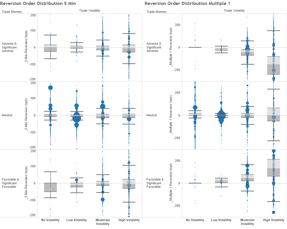
Figure 1: Reversion Distributions by Momentum and Volatility Environments - Shorter Horizon

(Figures 1; 2) show the reversion in prices after an order has completed, broken down by volatility and momentum buckets which are defined below. The full order sample includes 148,812 institutional orders from 70+ countries with 17 countries having at-least a thousand orders each . This global sample illustrates that the phenomenon is not restricted to any single country. The reversion is based on two measures:

1. In time, 5 minutes and 60 minutes after an order has completed.

2. In multiples of the order size, one times and five times the size of the order.

The five Trade Momentum buckets are based on the side adjusted percentage return during the order’s trading interval:

1. Significant Adverse (<-2%)

2. Adverse (-1/3% thru -2%)

3. Neutral (-1/3% thru +1/3%)

4. Favorable (+1/3% thru 2%)

5. Significant Favorable (>+2%)

The four Trade Volatility buckets are based on the coefficient of variationof prices during the execution horizon:

1. High Volatility (>0.0050)

2. Moderate Volatility (0.0010 thru 0.0050)

3. Low Volatility (0.000000000000001 thru 0.0010)

4. No Volatility (<= 0.000000000000001)

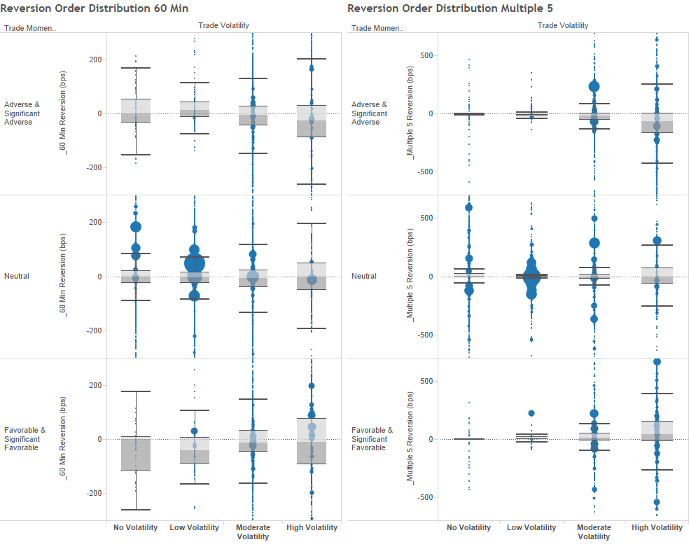
Figure 2: Reversion Distributions by Momentum and Volatility Environments - Longer Horizon

(Figure 1) has two reversion indicators: 5 minutes on the left half and one times the order size on the right half. (Figure 2) also has two reversion indicators: 60 minutes on the left half and five times the order size on the right half. For each reversion indicator, there are four volatility buckets on the X-axis and three momentum buckets are on the Y-axis since we club together the orders in the Significant Adverse and Adverse buckets; and the Significant Favorable and Favorable buckets. Each order from the sample will be represented as a bubble in all four reversion indicators and within one of the four volatility buckets and one of the three momentum buckets. The size of the bubbles indicates the relative magnitude of the order and its position on the vertical axis signifies the reversion amount in basis points. The box (grey region between two horizontal lines) and the whisker (two horizontal lines separated by a vertical line) capture the areas where 25% and 75% of the sample resides.

Not surprisingly, the momentum and reversion are higher in periods of greater volatility, as seen more clearly from the measures based on multiples of the order size (right half of Figures 1; 2). The higher volatility accentuates the efforts required to trade in such an environment. This illustrates the issue that traders face and the optimization process that is followed where they try to benefit from positive momentum and try to avoid adverse momentum by trading more when adverse momentum is anticipated, while being conscious of the level of volatility.

2.2 Related Literature

Building on the foundation laid by (Bertsimas & Lo 1998), another popular way to decompose trading costs is into temporary and permanent impact (see, Almgren & Chriss 2001; Almgren 2003; and Almgren, Thum, Hauptmann & Li 2005). While the theory behind this approach is extremely elegant and considers both linear and nonlinear functions of the variables for estimating the impact, a practical way to compute it requires measuring the price a certain interval after the order. This interval is ambiguous and could lead to lower accuracy while using this measure.

More recent extensions include: minimizing the mean and variance of the costs of trading for the case of market orders only to derive explicit formulas for the optimal trading strategies (Huberman & Stanzl 2005); considering quadratic variation as a reasonable risk measure rather than variance, (Forsyth, Kennedy, Tse & Windcliff 2012); the problem faced by an investor who must liquidate a given basket of assets over a finite time horizon (Schied, Schöneborn & Tehranchi 2010); (Almgren & Lorenz 2007) derive optimal strategies where the execution accelerates when the price moves in the trader’s favor, and slows when the price moves adversely;

(Schied & Schöneborn 2009) use a stochastic control approach, building upon the continuous time model of (Almgren 2003), and show that the value function and optimal control satisfy certain nonlinear parabolic partial differential equations that can be solved numerically. (Kato 2014) develops a mathematical model of optimal execution, by formulating it as a stochastic control problem in the continuous time domain. (Gatheral & Schied 2011) find a closed-form solution for the optimal trade execution strategy in the Almgren-Chriss framework assuming the underlying unaffected stock price (stock price before the impact or before the transaction occurs) process is a GBM; (Schied 2013) investigates the robustness of this strategy with respect to misspecification of the law of the underlying unaffected stock price process. (Guo & Zervos 2015) study the optimal execution problem in the context of a continuous time model with multiplicative price impact, involving singular control rather than absolutely continuous control.

Building on empirical evidence (Lillo, Farmer & Mantegna 2003) that instantaneous market impact is a strongly concave function of the volume, well approximated by a power law function at least for trading rates that are not too high; (Curato, Gatheral & Lillo 2017) find that the discretized cost function exhibits a rugged landscape with many local minima separated by peaks. (Huberman & Stanzl 2004) provide theoretical arguments showing that in the absence of quasi-arbitrage (availability of a sequence of round-trip trades that generate infinite expected profits with an infinite Sharpe ratio, that is infinite expected profits per unit of risk), permanent price-impact functions must be linear; though empirical investigations suggest that the shape of the limit order book (LOB) can be more complex (Hopman 2007). (Gabaix, Gopikrishnan & Stanley 2006) present a theory in which spikes in trading volume and returns, and hence stock market volatility, are created by a combination of news and the trades of large investors explaining the power law distribution of price impact. (Brunnermeier & Pedersen 2005; Carlin, Lobo & Viswanathan 2007) are extensions to situations with several competing traders, wherein if one trader is forced to liquidate his holdings, other traders also sell creating downward price pressure and buy back the assets later at a lower price.

In contrast to many studies, where the dynamics of the asset price process is taken as a given fundamental, (Obizhaeva & Wang 2013) proposed a market impact model that derives its dynamics from an underlying model of a LOB. In this model, the ask part of the LOB consists of a uniform distribution of shares offered at prices higher than the current best ask price.

(Alfonsi, Fruth & Schied 2010) extend this by allowing for a general shape of the LOB defined via a given density function, which can accommodate empirically observed LOB shapes and obtain a nonlinear price impact of market orders. (Predoiu, Shaikhet & Shreve 2011) derive optimal strategies, (under a general shape of the LOB), that are a mixture of lump purchases and continuous purchases with the rate of purchase set to match the order book resilience. (Fruth, Schöneborn & Urusov 2014) analyze optimal strategies for a risk neutral investor when liquidity varies deterministically (liquidity is time dependent; depth and resilience can be independently time-dependent in contrast to the LOB model of Obizhaeva & Wang 2013) and find that in the case of extreme changes in liquidity, it can even be optimal to completely refrain from trading in periods of low liquidity. Empirical studies based on the LOB model are (Biais, Hillion & Spatt 1995; Potters & Bouchaud 2003; Bouchaud, Gefen, Potters & Wyart 2004; Weber & Rosenow 2005).

A related strand of literature looks at models of the LOB from the perspective of dealers seeking to submit optimal strategies (maximize the utility of total terminal wealth) of bid and ask orders. (Ho & Stoll 1981) analyze the optimal prices for a monopolistic dealer in a single stock when faced with a stochastic demand to trade, modeled by a continuous time Poisson jump process, and facing return uncertainty, modeled by diffusion processes. (Ho and Stoll 1980), consider the problem of dealers under competition (each dealer’s pricing strategy depends not only on his own current and expected inventory position and his other characteristics, but also on the current and expected inventory and other characteristics of the competitor) and show that the bid and ask prices are shown to be related to the reservation (or indifference) prices of the agents.

(Cont, Stoikov & Talreja 2010) describe a stylized model for the dynamics of a limit order book, where the order flow is described by independent Poisson processes, and estimate the model parameters from high-frequency order book time-series data from the Tokyo Stock Exchange. (Cont, Kukanov & Stoikov 2014) study the price impact of order book events - limit orders, market orders and cancellations - using the NYSE Trades and Quotes data for fifty randomly selected stocks. (Avellaneda & Stoikov 2008) combine the utility framework with the microstructure of actual limit order books, as described in the econo-physics literature, to infer reasonable arrival rates of buy and sell orders; (Du, Zhu & Zhao 2016) extend the price dynamics to follow a GBM in which the drift part is updated by Bayesian learning in the beginning of the transaction day to capture the trader’s estimate of other traders’ target sizes and directions.

(Cont & Kukanov 2017) focus on the order placement problem, which is to choose an order type - market or limit order - and which trading venue(s) to submit it to, when there are multiple alternatives. A numerical algorithm for solving the order placement problem in a general case is provided using a robust modification of the Robbins-Monro stochastic approximation technique (Robbins & Monro 1951; Nemirovski, Juditsky, Lan & Shapiro 2009). (Guo, de Larrard & Ruan 2017) derive optimal placement strategies for both static and dynamic cases (in the static case, as opposed to the dynamic case, a strategy is completely decided before execution takes place, that is at $t=0$, and is unchanged over the entire order internal), under a correlated random walk model, with mean-reversion for the best ask/bid price.

While our work focuses on separating impact and timing in the (Bertsimas & Lo 1998) framework; a natural and interesting continuation would be to extend this separation to models of the limit order book discussed above (Obizhaeva & Wang 2013).

Models of market impact and the design of better trading strategies are becoming an integral part of the present trend at automation and the increasing use of algorithms. (Jain 2005) assembles the dates of announcement and actual introduction of electronic trading by the leading exchange of 120 countries to examine the long term and medium term impact of automation. He finds that automation of trading on a stock exchange has a long-term impact on listed firms’ cost of equity. (Hendershott, Jones & Menkveld 2011) perform an empirical study on New York Stock Exchange stocks and find that algorithmic trading and liquidity are positively related. It is worth noting a contrasting result from an earlier study. (Venkataraman 2001) compares securities on the New York Stock Exchange (NYSE) (a floor-based trading structure with human intermediaries, specialists and floor brokers) and the Paris Bourse (automated limit-order trading structure). He finds that execution costs might be higher on automated venues even after controlling for differences in adverse selection, relative tick size, and economic attributes. This means fully automated exchanges, which anecdotally seems to be the way ahead, need to take special care to formulate rules to help liquidity providers better control the risks of order exposure.

What this also means is that, the design of better strategies and models is crucial to survive and thrive in this continuing trend at automation. Our paper aims to fill the gap in existing models of trading costs, which are theoretically elegant but are not readily applicable to real life trading situations, since they do not allow participants to gauge how they are performing in comparison to the other participants with whom they are competing for liquidity. Our models have a strong theoretical foundation but they can be applied to actual trading situations due to the insights they provide to participants. In addition, our numerical framework can be be used to obtain optimal execution schedules under any law of motion of prices.

3 Dynamic Recursive Trading Cost Model

A dynamic programming approach lends itself naturally to modeling optimal execution strategies. (Bertsimas & Lo 1998) start with a simple arithmetic random walk for the law of motion of prices and later extend it to a Geometric Brownian motion. Their approach and extensions result in closed form or numerical solutions for many scenarios (section 2.2). As (section 2.2) also highlights, existing dynamic programming methods to optimizing trading costs and execution scheduling are of limited use to practitioners and traders since they do not provide a way for them to understand how their actions at each stage would affect the price (as opposed to the combined effect of everyone else or the market) and thereby pointing out specific aspects of the system that they can hope to influence. Hence, we start with the benchmark dynamic programming problem (section 3.1) and modify the reward function in the Bellman equation to suit our innovation in later sections.

The objective of any trading program is to formulate a trading trajectory, or a list of total pending shares, $W_{1},...,W_{T+1}$ at the end of each time period. Here, $T$ is the total duration of trading. For simplicity, time in measured in unit intervals giving, $t=1,2,...,T$. $W_{t}$ then becomes the number of units that we still need to trade at time $t$. $\bar{S}$ is the total number of shares that need to be traded. Conditions ($W_{1}=\bar{S}\;\&\;W_{T+1}=0$ ) together imply that $\bar{S}$ must be executed by period $T$ (this is an assumption that there will be no unexecuted shares once the total time duration is completed; this is a constraint to be satisfied while seeking the trading schedule).

A trading strategy can equivalently be represented by the list of executions completed, $S_{1},...,S_{T}$. $S_{t}$ is the number of shares acquired in period $t$ at price $P_{t}$. Clearly, $\bar{S}=\underset{j=1}{\overset{T}{\sum}}S_{j}$. This gives, $W_{t}=W_{t-1}-S_{t-1}$ or $S_{t-1}=W_{t-1}-W_{t}$ is the number of units traded between times $t-1$ and $t$ at price $P_{t-1}$. That is we go from $W_{t-1}$ unexecuted shares at time period $t-1$ to $W_{t}$ remaining shares at time $t$ by filling $S_{t-1}$ shares at price $P_{t-1}$. $W_{t}$ and $S_{t}$ are related as below.

$$W_{t}=\bar{S}-\underset{j=1}{\overset{t-1}{\sum}}S_{j}=\underset{j=t}{\overset{T}{\sum}}S_{j}\qquad,t=1,...,T.$$ (1)

3.1 Benchmark Dynamic Programming Model

This is the simplest scenario where the trader would try to minimize the overall acquisition value of his holdings. This is also the benchmark scenario in (Bertsimas & Lo 1998). In this case, securities are being bought. It is then logical to set a no sales constraint when the objective is to buy securities. The baseline objective function and constraints are written as,

$$\underset{\left\{S_{t}\right\}}{\min}\>E_{1}\left[\sum_{t=1}^{T}S_{t}P_{t}\right]$$ (2)

$$\sum_{t=1}^{T}S_{t}=\bar{S}\;,S_{t}\geq 0\;,W_{1}=\bar{S},\;W_{T+1}=0\;,\;W_{t}=W_{t-1}-S_{t-1}$$ (3)

The law of motion of price, $P_{t}$ for the buy scenario can be written as,

$$P_{t}=P_{t-1}+\theta S_{t}+\varepsilon_{t}\;,\theta>0\>,E\left[\varepsilon_{t}\left|S_{t},P_{t-1}\right.\right]=0$$ (4)

$$\varepsilon_{t}\sim N\left(0,\sigma_{\varepsilon}^{2}\right)\equiv\text{Zero Mean IID (Independent Identically Distributed) random shock or white noise}$$

We also follow the convention that the shares are positive when we buy and negative when we sell. The law of motion of price, $P_{t}$ for the sell scenario then becomes,

$$P_{t}=P_{t-1}-\theta S_{t}+\varepsilon_{t}\;,\theta>0\>,E\left[\varepsilon_{t}\left|S_{t},P_{t-1}\right.\right]=0$$ (5)

This price evolution and convention for the buy and sell scenarios ensures that the buyer and the seller have the same price. A trade happens only when the buyer and seller agree upon the price and they both face the same shock in this case. In the rest of the discussion we only consider the price evolution for the buy scenario since this treatment applies with simple modifications when securities are sold.

The law of motion includes two distinct components: the dynamics of $P_{t}$ in the absence of our trade, (the trades of other may be causing prices to fluctuate) and the impact that our trade of $S_{t}$ shares has on the execution price $P_{t}$. This simple price change relationship assumes that the former component is given by an arithmetic random walk and the latter component is a linear function of trade size so that a purchase of $S_{t}$ shares may be executed at the prevailing price plus an impact premium of $\theta S_{t}$. Here, $\theta$ captures the effect of transaction size on the price. In the absence of this transaction, the price process evolves as a pure arithmetic random walk. This then implies that from any participants view, the sum of all the price movements or the new price levels established by all other participants evolves as a random walk. For simplicity, we ignore the no sales constraint, $S_{t}\geq 0$.

The Bellman equation is based on the observation that a solution or optimal control $\left\{S_{1}^{*},S_{2}^{*},...,S_{T}^{*}\right\}$ must also be optimal for the remaining program at every intermediate time $t.$ That is, for every $t,$ $1<t<T$ the sequence $\left\{S_{t}^{*},S_{t+1}^{*},...,S_{T}^{*}\right\}$ must still be optimal for the remaining program $E_{t}\left[\sum_{k=t}^{T}P_{k}S_{k}\right]$. The below relates the optimal value of the objective function $V_{t}$ in period $t$ to its optimal value in period $t+1:$

$$V_{t}\left(P_{t-1},W_{t}\right)=\underset{\left\{S_{t}\right\}}{\min}\>E_{t}\left[P_{t}S_{t}+V_{t+1}\left(P_{t},W_{t+1}\right)\right]$$ (6)

3.2 Terminology and High-Level Mathematical Expressions

We now introduce some terminology used throughout the discussion. We also provide simple mathematical expressions to convey the intuition behind our methodology. (Sections 4; 6) have a rigorous mathematical treatment.

1. Total Slippage: The overall price move on the security during the order duration. This is also a proxy for the implementation shortfall (Perold 1988; Treynor 1981; section 3.3).

2. Market Impact (MI): The price moves caused by the executions that comprise the order under consideration. In short, the MI is a proxy for the impact on the price from the liquidity demands of an order. This metric is generally negative or zero since in most cases the best impact we can have is usually no impact.

3. Market Timing: The price moves that happen due to the combined effect of all the other market participants during the order duration.

4. Market Impact Estimate (MIE): An estimate of the Market Impact, (point 2), based on recent market conditions. The MIE calculation is the result of a simulation which considers the number of executions required to fill an order and the price moves encountered while filling this order. It depends on the market micro-structure as captured by the trading volume and the price probability distribution that factors upticks and down-ticks. This simulation can be controlled with certain parameters that dictate the liquidity demanded on the order, the style of trading, order duration, start and end of trading times. In short, the MIE is an estimated proxy for the impact on the price from the liquidity demands of an order.

5. Market Timing Estimate (MTE): This is an estimate of the Market Timing, (point 3), based on recent market conditions. The MTE calculation is highly dependent on the price volatility and hence the longer the duration, the higher we can expect the timing to be. It is helpful to consider an upper bound and lower bound for the MTE or a range for the MTE for the duration of trading.

3.3 The Implementation Shortfall

As a refresher, the total slippage or implementation shortfall is derived below with the understanding that we need to use the Expectation operator when we are working with estimates or future prices. $P_{0}$ can be any reference price or benchmark used to measure the slippage. It is generally taken to be the arrival price or the price at which the portfolio manager would like to complete the purchase of the portfolio.

$$\text{Paper Return}=\bar{S}P_{T}-\bar{S}P_{0}$$ (7)

$$\text{Real Portfolio Return}=\bar{S}P_{T}-\left(\sum_{t=1}^{T}S_{t}P_{t}\right)$$ (8)

Implementation Shortfall $$=\text{Paper Return}-\text{Real Portfolio Return}$$ (9)

$$=\left(\sum_{t=1}^{T}S_{t}P_{t}\right)-\bar{S}P_{0}$$ (10)

This can be written as,

Implementation Shortfall $$=\left(\sum_{t=1}^{T}S_{t}P_{t}\right)-\bar{S}P_{0}$$ (11)

$$=\left(\sum_{t=1}^{T}S_{t}P_{t}\right)-P_{0}\left(\sum_{t=1}^{T}S_{t}\right)$$ (12)

$$=S_{1}\left(P_{1}-P_{0}\right)+S_{2}\left(P_{2}-P_{0}\right)+...+S_{T}\left(P_{T}-P_{0}\right)$$ (13)

Implementation Shortfall $$=S_{1}\left(P_{1}-P_{0}\right)$$ (14)

$$+S_{2}\left(P_{2}-P_{1}\right)+S_{2}\left(P_{1}-P_{0}\right)$$ (15)

$$+S_{3}\left(P_{3}-P_{2}\right)+S_{3}\left(P_{2}-P_{1}\right)+S_{3}\left(P_{1}-P_{0}\right)+\;...\;$$ (16)

$$+S_{T}\left(P_{T}-P_{T-1}\right)+S_{T}\left(P_{T-1}-P_{T-2}\right)+...+S_{T}\left(P_{1}-P_{0}\right)$$ (17)

The innovation we introduce would incorporate our earlier discussion about breaking the total impact or slippage, Implementation Shortfall, into the part from the participants own decision process, Market Impact, and the part from the decision process of all other participants, Market Timing. This Market Impact, would capture the actions of the participant, since at each stage the penalty a participant incurs should only be the price jump caused by their own trades and that is what any participant can hope to minimize. A subtle point is that the Market Impact portion need only be added up when new price levels are established. If the price moves down and moves back up (after having gone up once earlier and having been already counted in the Impact), we need not consider the later moves in the Market Impact (and hence implicitly left out from the Market Timing as well). This alternate measure, which does not consider subsequent price moves down and up after having gone up once earlier, would only account for the net move in the prices but would not show the full extent of aggressiveness and the push and pull between market participants and hence is not considered here, though it can be useful to know and can be easily incorporated while running simulations. We discuss two formulations of our measure of the Market Impact in (sections 3.4; 3.5). The reason for calling them simple and complex will become apparent as we continue the discussion.

3.4 Market Impact Simple Formulation

The simple market impact formulation does not consider the impact of the new price level established on all the future trades that are yet to be done. From a theoretical perspective it is useful to study this since it provides a closed form solution and illustrates the immense practical application of separating impact and timing. This approach can be a useful aid in markets that are clearly not trending and where the order size is relatively small compared to the overall volume traded, ensuring that any new price level established does not linger on for too long and prices gets reestablished due to the trades of other participants. This property is akin to checking that shocks to the system do not take long to dissipate and equilibrium levels (or rather new pseudo equilibrium levels) are restored quickly. Our measure of the Market Impact then becomes,

$$\text{Market Impact}=\sum_{t=1}^{T}\left\{\max\left[\left(P_{t}-P_{t-1}\right),0\right]S_{t}\right\}$$ (18)

The Market Timing is then given by,

Market Timing $$=\text{Implementation Shortfall}-\text{\text{Market Impact}}$$ (19)

$$=\left(\sum_{t=1}^{T}S_{t}P_{t}\right)-\bar{S}P_{0}-\sum_{t=1}^{T}\left\{\max\left[\left(P_{t}-P_{t-1}\right),0\right]S_{t}\right\}$$ (20)

(Appendix 11.2) has some illustrative examples.

3.5 Market Impact Complex Formulation

Another measure of the Market Impact can be formulated as below which represents the idea that when a participant seeks liquidity and establishes a new price level, all the pending shares or the unexecuted program is affected by this new price level. This is a more realistic approach since the action now will explicitly affect the shares that are not yet executed. This measure can be written as,

$$\text{Market Impact}=\sum_{t=1}^{T}\left\{\max\left[\left(P_{t}-P_{t-1}\right),0\right]W_{t}\right\}$$ (21)

The Market Timing is then given by,

Market Timing $$=\text{Implementation Shortfall}-\text{\text{Market Impact}}$$ (22)

$$=\left(\sum_{t=1}^{T}S_{t}P_{t}\right)-\bar{S}P_{0}-\sum_{t=1}^{T}\left\{\max\left[\left(P_{t}-P_{t-1}\right),0\right]W_{t}\right\}$$ (23)

(Appendix 11.3) has some illustrative examples.

3.6 Trading Costs as a Zero Sum Game

A formal study of trading costs in the financial markets using the tools of game theory can lead to many interesting conclusions. Even without a set up specific to game theory one of the results we obtain, though fairly evident but perhaps surprising given the extent of trading that takes place in today’s markets, is that in any given time period the sum of market impact and the sum of market timing across all market participants equals zero.

This is immediately obvious in the case that there are only two participants (one is the buyer, the other is the seller and without two participants we do not have a market or a trade) and there is only one single interval, since negative implementation shortfall for the buyer shows up as positive implementation shortfall for the seller; the impact for the buyer shows up as timing for the seller and vice versa. We note that the total amount bought in any interval is equal to the total amount sold. When there are more than two participants and multiple intervals, if we consider the actions in each interval and add up the impact and timing figures across everyone, it shows the zero sum nature of the trading game . The result holds for both the simple and complex formulations of market impact.

Theorem 1.

Trading costs are a zero sum game. The sum of market impact and market timing across all participants, in any given time interval, should equal zero.

$$\text{Total Market Impact}+\text{Total \text{Market Timing}}=0$$

Proof.

Appendix 12.1. ∎

Though we refrain from a longer discussion for the sake of brevity; it should be immediately apparent that the zero sum nature of trading costs is applicable outside the financial markets to all manner of trades within international / intra-national finance and the exchange of all types of goods and services. Another aspect we point out is the difference in the proportion of timing and impact between financial markets and trading in other products. The relative ease with which products can be liquidated and / or the extent to which they are either consumption or investment goods, affects this property (Kashyap 2014).

4 Alternative and Practical Dynamic Market Impact Model

In this section, we discuss the benchmark law of motion of prices while optimizing the simple and complex market impact formulations. Other extensions of the law of motion of prices are considered in Section 6 in the Appendix. Prices can be negative under the benchmark law of motion. Section 6.3 in the Appendix shows how to set up the numerical solution when the no impact prices evolve as a Geometric Brownian Motion, which ensures that prices remain positive under mild restrictions on the parameters.

4.1 Simple Formulation of the Benchmark Law of Price Motion

Incorporating the Simple Market Impact formulation from section 3.4, the benchmark objective function and the Bellman equation from section 3.1 can be modified as,

$$\underset{\left\{S_{t}\right\}}{\min}\>E_{1}\left[\sum_{t=1}^{T}\left\{\max\left[\left(P_{t}-P_{t-1}\right),0\right]S_{t}\right\}\right]$$ (24)

$$\sum_{t=1}^{T}S_{t}=\bar{S}\;,S_{t}\geq 0\;,W_{1}=\bar{S},\;W_{T+1}=0\;,\;W_{t}=W_{t-1}-S_{t-1}$$ (25)

$$P_{t}=P_{t-1}+\theta S_{t}+\varepsilon_{t}\;,\theta>0\>,E\left[\varepsilon_{t}\left|S_{t},P_{t-1}\right.\right]=0\;,\;\varepsilon_{t}\sim N\left(0,\sigma_{\varepsilon}^{2}\right)$$ (26)

The Bellman equation then becomes,

$$V_{t}\left(P_{t-1},W_{t}\right)=\underset{\left\{S_{t}\right\}}{\min}\>E_{t}\left[\max\left\{\left(P_{t}-P_{t-1}\right),0\right\}S_{t}+V_{t+1}\left(P_{t},W_{t+1}\right)\right]$$ (27)

One additional constraint that is necessary is to restrict the amount of shares available for trading in any time period when the price in that time period drops in comparison to the previous time period. The algorithm in section 5 shows how these constraints can be set. This is a practical consideration, since a drop in price is impact for the sellers and timing for the buyers (as a reminder, we are buyers). Hence when the price decreases in comparison to the previous time period, the amount of shares or liquidity is limited and the seller decides how much to make available. When prices are rising, we can justify not having that criteria, since the buyer can bid up the price and decide how much impact they want to incur. A more thorough approach would ensure that the liquidity follows a process of its own and captures this dynamic of sellers and buyers being able to prop the prices from falling further or rising higher respectively. In the extension we consider in section 6.4, some of these aspects can be factored in.

By starting at the end, (time $T$) and applying the modified Bellman equation, the law of motion for $P_{t}$, the relation between pending and executed shares, and the boundary conditions recursively, the optimal control can be derived as functions of the state variables that characterize the information that the investor must have to make his decision in each period. In particular, the optimal value function, $V_{T}\left(\cdots\right)$, as a function of the two state variables $P_{T-1}$ and $W_{T}$ is given by,

$$V_{T}\left(P_{T-1},W_{T}\right)=\underset{\left\{S_{T}\right\}}{\min}\>E_{T}\left[\max\left\{\left(P_{T}-P_{T-1}\right),0\right\}S_{T}\right]$$ (28)

Here, the remaining shares $W_{T+1}$ must be zero since there is no choice but to execute all the remaining shares, $W_{T}$. We then have the optimal trade size, $S_{T}^{*}=W_{T}$ and an expression for $V_{T}$ as,

$$V_{T}\left(P_{T-1},W_{T}\right)=E_{T}\left[\max\left\{\left(\theta W_{T}+\varepsilon_{T}\right),0\right\}W_{T}\right]$$ (29)

Proposition 1.

The value function for the last but one time period is convex and can be written as,

$$V_{T-1}\left(P_{T-2},W_{T-1}\right) = \underset{\left\{S_{T-1}\right\}}{\min}\left[S_{T-1}\sigma_{\varepsilon}\psi\left(\xi S_{T-1}\right)+\left(W_{T-1}-S_{T-1}\right)\sigma_{\varepsilon}\psi\left\{\xi\left(W_{T-1}-S_{T-1}\right)\right\}\right]$$

$$\text{Here, }\psi\left(u\right)=u+\phi\left(u\right)/\Phi\left(u\right)\;,\;\xi=\frac{\theta}{\sigma_{\varepsilon}},$$

Also, $\phi$ and $\mathbf{\Phi}$ are the standard normal Probability Density Function, PDF, and Cumulative Distribution Function CDF, respectively.

Proof.

Appendix 12.2. ∎

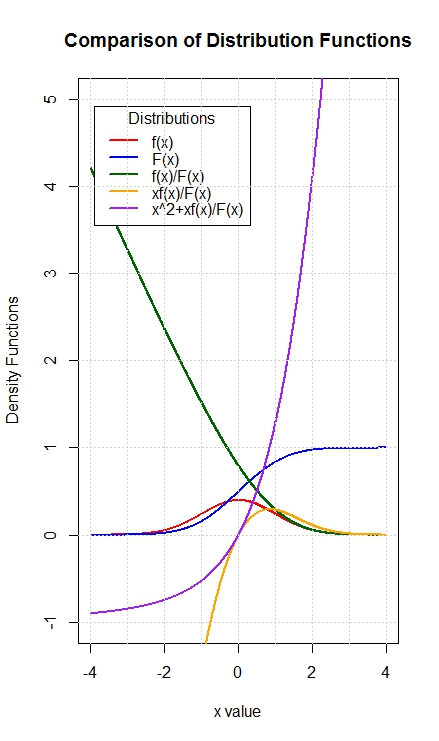
Figure 3: Convexity of Distribution Functions

Figure 3 illustrates the shape of some combinations of the distribution functions that we are working with. For the value function we have, the condition for convexity can be derived as $\theta>\left(3\sigma_{\varepsilon}/4\right)$.

Proposition 2.

The number of shares to be executed in each time period follows a linear law. $S_{T-1}^{*}=W_{T-1}^{*}/2,\quad\ldots\quad,S_{T-K-1}^{*}=W_{T-K-1}/\left(K+2\right)$ $,S_{T-K}^{*}=W_{T-K}/\left(K+1\right)$ and the corresponding value functions are,

$$V_{T-K-1}\left(P_{T-K-2},W_{T-K-1}\right)=\sigma_{\varepsilon}W_{T-K-1}\left[\frac{\theta}{\sigma_{\varepsilon}}\frac{W_{T-K-1}}{\left(K+2\right)}+\frac{\phi\left(\frac{\theta}{\sigma_{\varepsilon}}\frac{W_{T-K-1}}{\left(K+2\right)}\right)}{\Phi\left(\frac{\theta}{\sigma_{\varepsilon}}\frac{W_{T-K-1}}{\left(K+2\right)}\right)}\right]$$

Proof.

Appendix 12.3 ∎

We can see that a minimum exists at each stage. The simple solution follows from the linear rule where the price impact $\theta S_{t}$ does not depend on either the prevailing price, $P_{t-1}$, or the size of the unexecuted order $W_{t}$ and hence the price impact function is the same in each period and independent from one period to the next. It is easily shown that, $S_{1}^{*}=S_{2}^{*}=\cdots=S_{T}^{*}=\bar{S}/T$. This simply means that the best execution strategy is simply to divide the total order or the total shares $\bar{S}$ into $T$ equal amounts and trade them at regular intervals. (Bertsimas & Lo 1998) has a more detailed discussion. Supposing a closed form solution was absent, we could approximate the solution (numerically solved) using $S_{T-1}^{*}\approx\xi_{0}+\xi_{1}W_{T-1}+\xi_{2}\left(W_{T-1}\right)^{2}$ or $S_{T-1}^{*}\approx\xi_{0}\left(W_{T-1}\right)^{\xi_{1}}$. We can also set $S_{T-1}^{*}\approx\omega_{1}\left(W_{T-1}\right)$ using any well behaved (continuous and differentiable) function, $\omega_{1}$. We could also include the last known price, $P_{t-1}$, or other state variables into the above approximation. We discuss this technique in detail including numerical examples in section 5. This numerical approximation approach is simple to implement and lends itself easily to solutions even in the more complex laws of motion to follow in section 6.

Going forward, to lighten the notion, we will drop the * superscript on the number of shares to be executed in each time period, $S_{T}^{*}$, where there is less likelihood of confusion.

4.2 Complex Formulation of the Benchmark Law of Price Motion

Incorporating the Complex Market Impact formulation from the earlier section 3.5, the objective function and the Bellman equation from section 3.1 can be modified as,

$$\underset{\left\{S_{t}\right\}}{\min}\>E_{1}\left[\sum_{t=1}^{T}\left\{\max\left[\left(P_{t}-P_{t-1}\right),0\right]W_{t}\right\}\right]$$ (30)

$$\sum_{t=1}^{T}S_{t}=\bar{S}\;,S_{t}\geq 0\;,W_{1}=\bar{S},\;W_{T+1}=0\;,\;W_{t}=W_{t-1}-S_{t-1}$$ (31)

$$P_{t}=P_{t-1}+\theta S_{t}+\varepsilon_{t}\;,\theta>0\>,E\left[\varepsilon_{t}\left|S_{t},P_{t-1}\right.\right]=0\;,\;\varepsilon_{t}\sim N\left(0,\sigma_{\varepsilon}^{2}\right)$$ (32)

The Bellman equation then becomes,

$$V_{t}\left(P_{t-1},W_{t}\right)=\underset{\left\{S_{t}\right\}}{\min}\>E_{t}\left[\max\left\{\left(P_{t}-P_{t-1}\right),0\right\}W_{t}+V_{t+1}\left(P_{t},W_{t+1}\right)\right]$$ (33)

The optimal value function, $V_{T}\left(\cdots\right)$, as a function of the two state variables $P_{T-1}$ and $W_{T}$ is given by,

$$V_{T}\left(P_{T-1},W_{T}\right)=\underset{\left\{S_{T}\right\}}{\min}\>E_{T}\left[\max\left\{\left(P_{T}-P_{T-1}\right),0\right\}W_{T}\right]$$ (34)

Here, the remaining shares $W_{T+1}$ must be zero since there is no choice but to execute all the remaining shares, $W_{T}$. We then have the optimal trade size, $S_{T}^{*}=W_{T}$ and an expression for $V_{T}$ as,

$$V_{T}\left(P_{T-1},W_{T}\right)=E_{T}\left[\max\left\{\left(\theta W_{T}+\varepsilon_{T}\right),0\right\}W_{T}\right]$$ (35)

Proposition 3.

The value function for the last but one time period is a convex function with a unique minimum, since it is the sum of the portions shown to be convex above (Proposition 1), another convex function and a linear component.

$$V_{T-1}\left(P_{T-2},W_{T-1}\right)=\underset{\left\{S_{T-1}\right\}}{\min}\left[W_{T-1}\sigma_{\varepsilon}\psi\left(\xi S_{T-1}\right)+\left(W_{T-1}-S_{T-1}\right)\sigma_{\varepsilon}\psi\left\{\xi\left(W_{T-1}-S_{T-1}\right)\right\}\right]$$

$$\text{Here, }\psi\left(u\right)=u+\phi\left(u\right)/\Phi\left(u\right)\;;\;\xi=\frac{\theta}{\sigma_{\varepsilon}}\;;\;\text{Note that, }W_{T-1}=S_{T-1}+W_{T}$$

The number of shares to be executed in subsequent time periods and the corresponding value function are obtained by solving,

$$W_{T-1}+\frac{\xi\left(W_{T-1}-S_{T-1}\right)^{2}\phi\left(\xi\left\{W_{T-1}-S_{T-1}\right\}\right)}{\Phi\left(\xi\left\{W_{T-1}-S_{T-1}\right\}\right)}+\left(W_{T-1}-S_{T-1}\right)\left[\frac{\phi\left(\xi\left\{W_{T-1}-S_{T-1}\right\}\right)}{\Phi\left(\xi\left\{W_{T-1}-S_{T-1}\right\}\right)}\right]^{2} =$$

$$2\left(W_{T-1}-S_{T-1}\right)+\frac{1}{\xi}\frac{\phi\left(\xi\left\{W_{T-1}-S_{T-1}\right\}\right)}{\Phi\left(\xi\left\{W_{T-1}-S_{T-1}\right\}\right)}+\frac{\xi W_{T-1}S_{T-1}\phi\left(\xi S_{T-1}\right)}{\Phi\left(\xi S_{T-1}\right)}+W_{T-1}\left[\frac{\phi\left(\xi S_{T-1}\right)}{\Phi\left(\xi S_{T-1}\right)}\right]^{2}$$

Proof.

Appendix 12.4. ∎

The simple rule established earlier, $S_{T-1}=W_{T-1}/2$, no longer applies here and we need numerical solutions at each stage. The complexity that gets included in this scenario, when we consider the rest of the unexecuted program into the market impact function, can be seen from this expression. We illustrate numerical techniques for obtaining optimal executions in section (5).

5 Numerical Framework for Optimal Execution

Below we develop a numerical framework that can provide optimal executions for any law of motion of prices. We specifically illustrate how we can solve the formulations from section 4 with this numerical technique. It should shortly become clear how this solution technique can be applied under any scenario of price changes including multiple sources of uncertainty. The central idea is similar to the American option pricing methodology (Longstaff & Schwartz 2001) that approximates the ex post realized payoffs from continuation on functions of the values of the state variables. In our case, we use least squares to approximate the conditional expectation of the number of shares to execute as a function of the state variables at each stage. The following points capture a high level essence of the algorithm.

5.1 Optimal Execution Algorithm

1. We create a matrix with the number of columns equal to the number of time periods and number of rows equal to the number of different price paths we desire (total number of simulations we are running). The first column in the matrix corresponds to the starting price, $P_{0}$, and the total number of shares to execute, $W_{1}$, before the start of the first time period, $T=1$. The second column has to hold the price, $P_{1}$, and the remaining number of shares to execute, $W_{2}$, before the start of the second time period, $T=2$. Each node (row and column) in the matrix has to contain the price and the number of shares to execute before the start of the corresponding time period.

2. The price at the start of any time period and the price innovation sampled from a suitable distribution ($\varepsilon_{t}\sim N\left(0,\sigma_{\varepsilon}^{2}\right)$ in our case) along with the number of shares executed during that time period incorporated into the corresponding law of motion give us the number of shares that still remain to be executed before the start of the next time period and the starting price point for the next time period. Any additional sources of uncertainty can also be included to obtain the next price level.

3. We randomly sample the remaining number of shares to be executed at the start of the second time period and thereafter from a uniform distribution by imposing suitable constraints. The upper limit for the uniform distribution can be the shares remaining at the start of the previous time period and the lower limit can be zero. During this process, the upper and lower limits for the uniform distribution can be changed to impose constraints on the minimum or maximum amounts we wish to execute during the previous time period.

4. Continuing this iteratively, we obtain a matrix where each node represents a different scenario of price and remaining number of shares to be executed before the start of the next time period. Each column contains many different combinations of price and remaining number of shares at the start of the corresponding time period.

5. Starting from the last time period, at each node, we compute the optimal number of shares to execute during that time period and later ones with complete knowledge of the innovations ($\varepsilon_{t}$) that unfold on that path, using well-known optimization techniques. For the complex impact function, we use the solnp package in R (Ghalanos, Theussl & Ghalanos 2012; Ye 1988); for the simple impact function, we allocate the remaining shares to the remaining time periods based on whether the corresponding innovations are negative and how negative they are.

   1. Considering the below example of obtaining the optimal executions when we are minimizing the complex impact function under the benchmark law of price motion, we write the objective function as,

      $$\underset{\left\{S_{t}\right\}}{\min}\left[\sum_{t=1}^{t=T}\left\{\max\left(\theta S_{t}+\varepsilon_{t},0\right)\left(\sum_{j=t}^{j=T}S_{j}\right)\right\}\right]$$ (36)

      Here, $\sum_{t=1}^{t=T}S_{t}=W_{1}$ ; $S_{t},W_{1}\geq 0$ and $\theta,\varepsilon_{t}\in R$, that is they are real numbers. Note that, $P_{t}-P_{t-1}=\theta S_{t}+\varepsilon_{t}$ for the benchmark law of price motion.

      • As an example, for $T=3$, the complete objective function will be,

        $$\underset{\left\{S_{1},S_{2},S_{3}\right\}}{\min}\left[\max\left(\theta S_{1}+\varepsilon_{1},0\right)\left(S_{1}+S_{2}+S_{3}\right)+\max\left(\theta S_{2}+\varepsilon_{2},0\right)\left(S_{2}+S_{3}\right)+\max\left(\theta S_{3}+\varepsilon_{3},0\right)\left(S_{3}\right)\right]$$ (37)

      • For the last time period, $T=3$, the optimal number of shares, $S_{3}^{*}=W_{3}$. Since this is the last time period we execute all the shares that are remaining at the start of the time period, $W_{3}$.

      • When we are at time period, $T=2$, we optimize $S_{2},S_{3}$ using the Rsolnp library such that the following function is minimized,

        $$\underset{\left\{S_{2},S_{3}\right\}}{\min}\left[\max\left(\theta S_{2}+\varepsilon_{2},0\right)\left(S_{2}+S_{3}\right)+\max\left(\theta S_{3}+\varepsilon_{3},0\right)\left(S_{3}\right)\right]$$ (38)

        Here, $\sum_{t=2}^{t=3}S_{t}=W_{2}$ ; $W_{2}$ would have a different value on each price path or for each row in our matrix and we need to perform this optimization exercise on each simulation path.

      • When we are at time period, $T=1$, we optimize $S_{1,}S_{2},S_{3}$ using the Rsolnp library such that the following function is minimized. This is the same as our complete optimization objective in Eq: 37.

        $$\underset{\left\{S_{1},S_{2},S_{3}\right\}}{\min}\left[\max\left(\theta S_{1}+\varepsilon_{1},0\right)\left(S_{1}+S_{2}+S_{3}\right)+\max\left(\theta S_{2}+\varepsilon_{2},0\right)\left(S_{2}+S_{3}\right)+\max\left(\theta S_{3}+\varepsilon_{3},0\right)\left(S_{3}\right)\right]$$ (39)

        Here, $\sum_{t=1}^{t=3}S_{t}=W_{1}$ ; $W_{1}$ is the total number of shares we start with and it would have a different value on each price path or for each row in our matrix. We need to perform this optimization on each simulation path.

      • If there are $N$ simulation price paths and $T$ time periods we need to make a total of $N*\left(T-1\right)$ calls to the Rsolnp routine.

   2. Considering the below example of obtaining the optimal executions when we are minimizing the simple impact function under the benchmark law of price motion, we write the objective function as,

      $$\underset{\left\{S_{t}\right\}}{\min}\left[\sum_{t=1}^{t=T}\left\{\max\left(\theta S_{t}+\varepsilon_{t},0\right)\left(S_{t}\right)\right\}\right]$$ (40)

      Here, $\sum_{t=1}^{t=T}S_{t}=W_{1}$ ; $S_{t},W_{1}\geq 0$ and $\theta,\varepsilon_{t}\in R$, that is they are real numbers. Note that, $P_{t}-P_{t-1}=\theta S_{t}+\varepsilon_{t}$

      • As an example, for $T=3$ the full objective function can be written as,

        $$\underset{\left\{S_{1},S_{2},S_{3}\right\}}{\min}\left[\max\left(\theta S_{1}+\varepsilon_{1},0\right)\left(S_{1}\right)+\max\left(\theta S_{2}+\varepsilon_{2},0\right)\left(S_{2}\right)+\max\left(\theta S_{3}+\varepsilon_{3},0\right)\left(S_{3}\right)\right]$$ (41)

      • For the last time period, $T=3$, the optimal number of shares, $S_{3}^{*}=S_{3}$.

      • When we are time period, $T=2,$ we optimize $S_{2},S_{3}$ such that the following function is minimized,

        $$\underset{\left\{S_{2},S_{3}\right\}}{\min}\left[\max\left(\theta S_{2}+\varepsilon_{2},0\right)\left(S_{2}\right)+\max\left(\theta S_{3}+\varepsilon_{3},0\right)\left(S_{3}\right)\right]$$ (42)

        Here, $\sum_{t=2}^{t=3}S_{t}=W_{2}$ ; $W_{2}$ would have a different value on each price path simulation or for each row in our matrix. The remaining shares $W_{2}$ are distributed to time periods that have negative innovations, starting with earlier time periods, until the execution size times the impact parameter $\theta$ plus the innovation equals zero for a particular time period. When this condition is satisfied, we incur zero impact $\left\{\theta S_{t}+\varepsilon_{t}=0\Rightarrow P_{t}-P_{t-1}=0\right\}$. After the execution size times the impact parameter $\theta$ plus the innovation equals zero for all time periods, any further leftover shares are allocated, while giving precedence to earlier time periods and then allocating to subsequent time periods, up-to the maximum execution limit for each time period, since the execution of these shares will cause an equal jump up in the prices (having an equal impact in the objective function) and it is better to execute sooner rather than later.

      • When we are at time period, $T=1$, we optimize $S_{1,}S_{2},S_{3}$ such that the following function is minimized. This is the same as our complete optimization objective in Eq: 41.

        $$\underset{\left\{S_{1},S_{2},S_{3}\right\}}{\min}\left[\max\left(\theta S_{1}+\varepsilon_{1},0\right)\left(S_{1}\right)+\max\left(\theta S_{2}+\varepsilon_{2},0\right)\left(S_{2}\right)+\max\left(\theta S_{3}+\varepsilon_{3},0\right)\left(S_{3}\right)\right]$$ (43)

        Here, $\sum_{t=1}^{t=3}S_{t}=W_{1}$ ; $W_{1}$ would have a different value on each price path simulation or for each row in our matrix. The remaining shares $W_{1}$ are distributed similar to the methodology described above.

6. We then run a regression across all the rows in the matrix (this is a cross sectional regression across the simulated paths) with the independent variables as the price, $P_{t-1}$, and the number of shares remaining to be executed before the time period starts, $W_{t}$, and the optimal number of shares to execute during that time period, $S_{t}$, as the dependent variable. It is to be understood that $W_{t}$, $P_{t-1}$, and $S_{t}$ denote the values of the variables across all the paths (total number of simulations) in our sample. We use a regression model such as the one below (Eq: 44). It should be clear that we can extend this to purely non-linear regressions or a combination of linear and non-linear components. Inclusion of additional variables such as spread, volume, number of trades, etc. are other possible extensions.

   $$E\left[S_{t}\left|W_{t,}P_{t-1}\right.\right]=\beta_{0}+\beta_{1}W_{t}+\beta_{2}W_{t}^{2}+\beta_{3}P_{t-1}+\beta_{4}P_{t-1}^{2}+\beta_{5}W_{t}P_{t-1}$$ (44)

   For $T=2$,

   $$E\left[S_{2}\left|W_{2,}P_{1}\right.\right]=\beta_{0}+\beta_{1}W_{2}+\beta_{2}W_{2}^{2}+\beta_{3}P_{1}+\beta_{4}P_{1}^{2}+\beta_{5}W_{2}P_{1}$$ (45)

7. Likewise, we continue backwards in time and obtain regression coefficients for each time period. The regression coefficients can then be used to calculate the optimal number of shares before the start of each time period. At each stage, we adjust the number of shares remaining before the time period starts based on the difference between the simulated number of shares to execute and the conditional expected value of the number of shares to execute as given by the above regression equation. For $T=2$, this adjusted number of remaining shares, $\hat{W}_{2}$, is given by,

   $$\hat{W}_{2}=S_{3}+\left(S_{2}-E\left[S_{2}\left|W_{2,}P_{1}\right.\right]\right)$$ (46)

5.2 Sample Results with Mean-Variance of Execution Costs

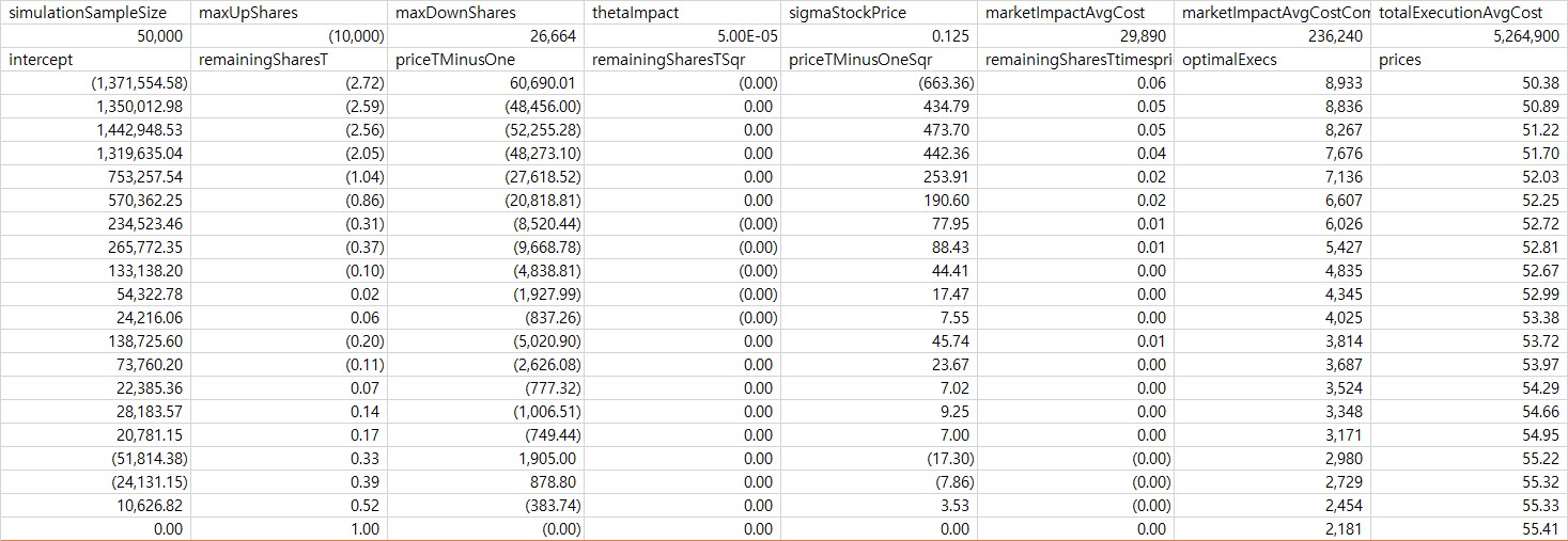
Figure 4: Complex Regression Coefficients and Optimal Executions

For the complex impact formulation, the table in (Figure 4) gives the regression coefficients when the number of time periods, $T=20$, the total number of shares to execute, $W_{1}=\bar{S}=100,000$ and the initial price, $P_{0}=50$. Starting from the initial time period in the first row, the optimal executions, the price path and other parameters are also shown. Unless specified otherwise all the parameter values are taken to be the same as the values in (Bertsimas & Lo 1998), to facilitate a proper comparison. (Figure 5) shows the optimal execution schedules under different levels of minimum and maximum number of shares to execute during each time period and different number of price paths or simulation counts.

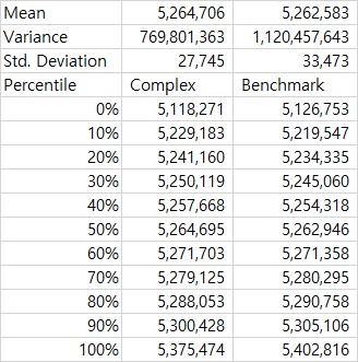
Figure 6: Mean / Variance / Percentile Comparison of Total Execution Costs

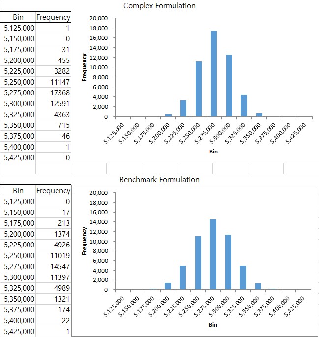
Figure 7: Histogram of Total Execution Costs

(Figure 6) compares the average and variance of the total impact costs of our numerical methodology with the benchmark case in (Bertsimas & Lo 1998; also termed the naive strategy), where the solution we get is to execute equal amount of shares in each time period. We report the mean and variance over a simulation sample of 50,000 price paths. We see that the benchmark case has a mean of around 5,262,583 which is comparable to the average execution cost of 5,264,706 using the complex formulation; but the variance is significantly lower using our methodology (769,801,363 in our case versus 1,120,457,643 in the benchmark model). (Figure 6) also reports the multiple of ten percentile values for the executions costs. (Figure 7) shows the histograms of the total costs under the two techniques (the top histogram is for the complex formulation). In addition, our methods are more realistic and adaptive, since the execution amounts change every-time we use it, as the market moves and as our trading progresses. Tailoring it to include additional state variables and capture other sources of uncertainty is relatively straightforward.

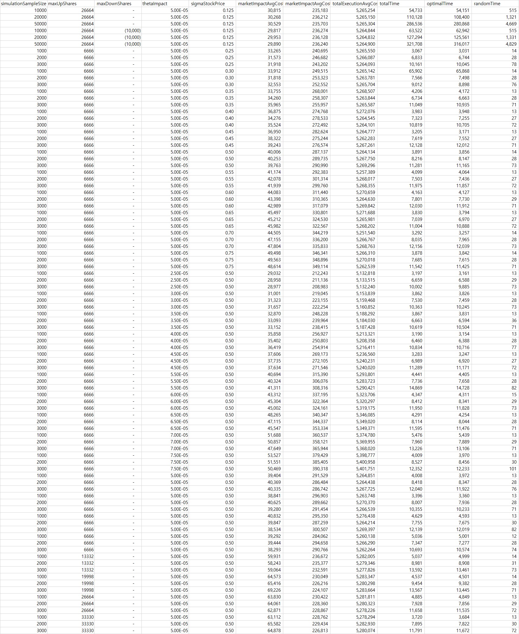
Figure 8: Complex Executions Costs for Different Parameters

Lastly to provide a better understanding of how execution costs change with changes in the different parameters, in (Figure 8) we provide the average of the total execution costs, the simple impact costs, the complex impact costs and the market timing costs across different parameter values, when we are optimizing the complex formulation of the market impact. We impose non-negativity constraints on the execution amounts while calculating the regression coefficient; later when we use the regression coefficients to calculate execution costs, we remove this restriction for some iterations; this parameter is captured as the maximum and minimum number of shares we can trade in any given time period.

The following values of the parameters are used in the computations: we vary the volatility of the stock price $\sigma_{\varepsilon}=\left\{0.125,0.25,0.30,0.35,0.40,0.45,0.50,0.55,0.60,0.65,0.70,0.75\right\}$, the impact parameter, $\theta=\left\{2.5,3.0,3.5,4.0,4.5,5.0,5.5,6.0,6.5,7.0,7.5\right\}$, the maximum and minimum number of shares we can execute in any given time period, i.e, the liquidity, $\left\{6666,13332,19998,26664,3333\right\}$ and $\left\{0,-10,000\right\}$, and the number of simulations, $\left\{50000,20000,10000,3000,2000,1000\right\}$. This gives a matrix of summary statistics with around 93 different combinations for which we calculate the regression coefficients, the simple market impact cost, the complex market impact cost and the total execution cost. It is immediately obvious that increasing the impact parameter, $\theta$, leads to an increase in the total executions costs (in Figure 8, when $\theta$ increases in this range, $\left\{2.5,3.0,3.5,4.0,4.5,5.0,5.5,6.0,6.5,7.0,7.5\right\}$, the corresponding total average costs are $\left\{5132240,5160852,5187428,5216411,5240020,5269296,5290421,5319175,5349371,5368020,5401751\right\}$. The increase in the price volatility and the liquidity in each time period do not show such a clear pattern and further investigation is warranted. But we can expect that the greater uncertainty due to higher price volatility and lack of liquidity, would force participants to trade greater amounts earlier in the trading horizon or as liquidity becomes available.

To calculate the regression coefficients in the quickest possible time, it would be helpful to build a decent amount of computing infrastructure. Since each price path can be developed independently and the only dependence across price paths is while doing the cross-sectional regressions, all the price paths and the optimization at each time period can be done using parallel processing technology. If there are 20 time periods and 1000 price paths, we would need to perform 20,000 Rsolnp optimization calls to compute all the regression coefficients for the complex impact formulation. This is the most time consuming portion of the algorithm and it is highly sensitive to the initial values provided for the routine. The calculation time increases significantly with the number of price paths and time periods; this increase is linear with the number of price paths but it can be more costly to perform the Rsolnp optimizations when the number of time periods increase. To make the calculation engine more robust we also build rudimentary intelligence, such that in case of any interruptions the system will revert back and resume the calculations from the last clean state that was reached. We ran our simulations on an Intel four core windows 10 machine with 4.00 Gigabytes RAM and 2.4 Gigahertz processor speed. In the summary statistics for each formulation we provide the time it takes to calculate all the coefficients (Figures 8; 11; 14).

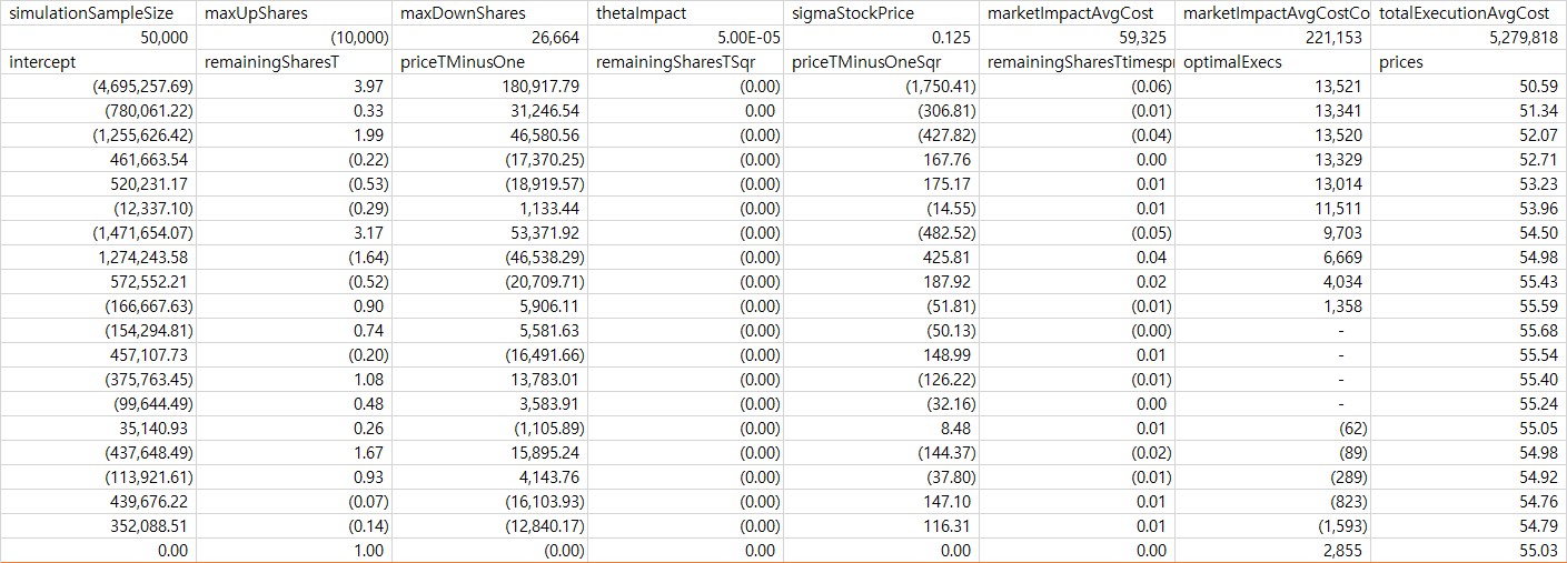
Figure 9: Simple Regression Coefficients and Optimal Executions

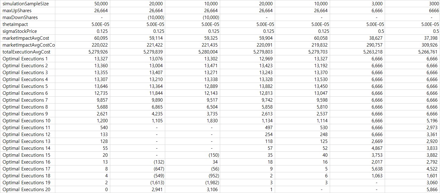
Figure 10: Simple Optimal Executions for Different Parameters

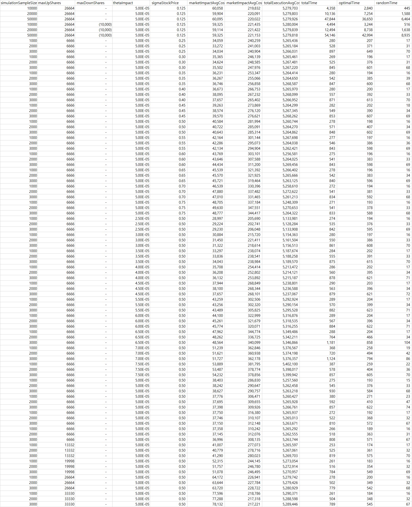
Figure 11: Simple Executions Costs for Different Parameters

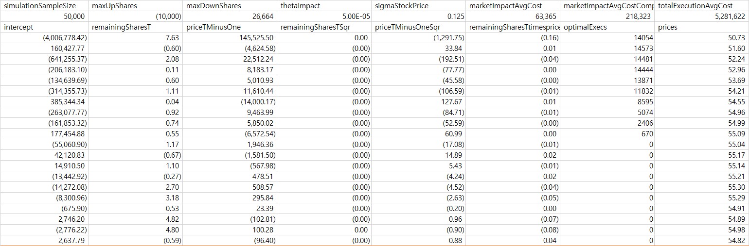
Figure 12: One Step Regression Coefficients and Optimal Executions

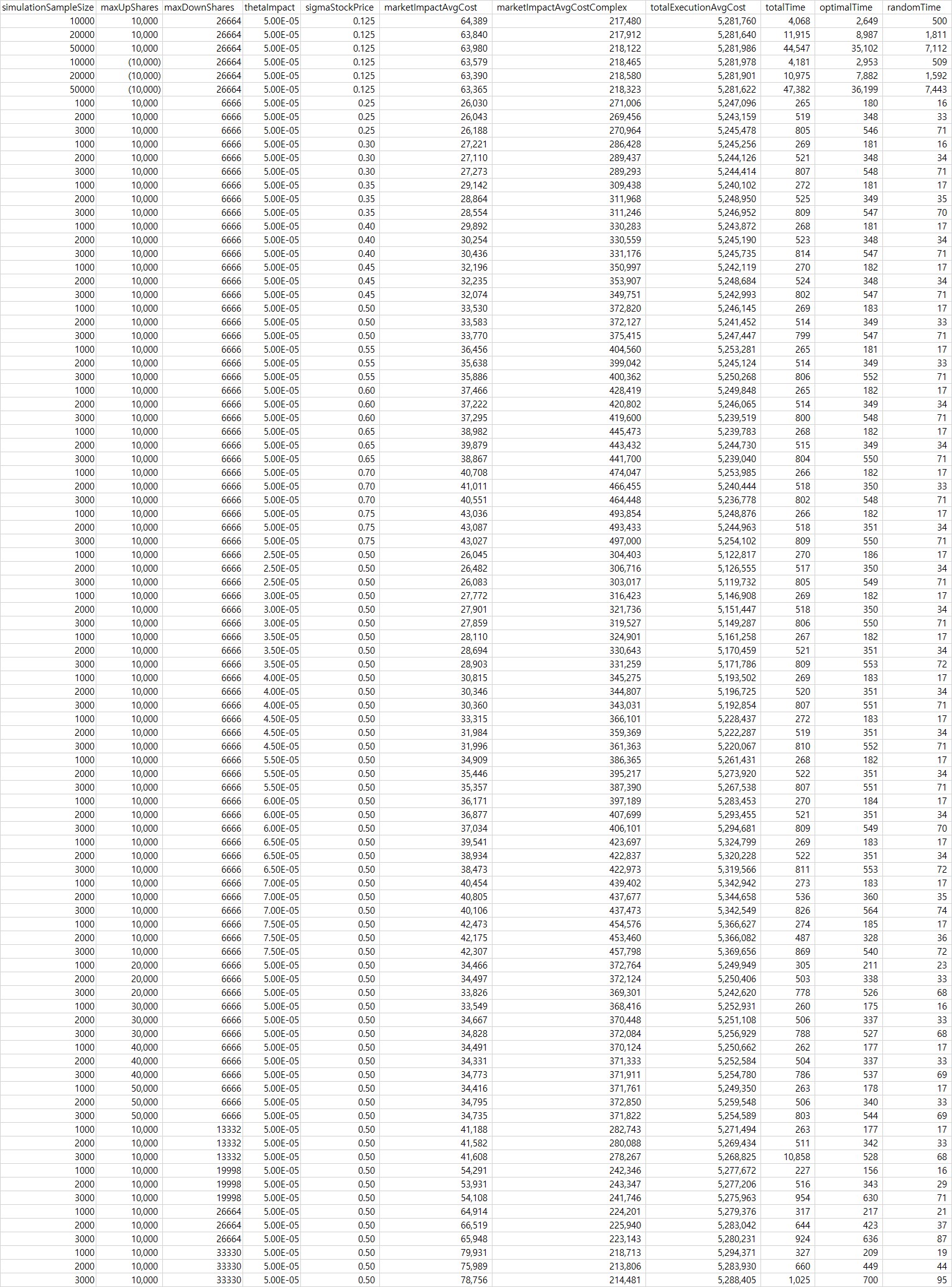
Figure 14: One Step Executions Costs for Different Parameters

To reduce the number of calculations, when we are looking to run optimal executions across hundreds of different securities, we could create groups of securities based on similarities in starting prices, volatilities and other parameters and compute regression coefficients for each group separately. Optimizing the simple impact formulation takes considerably less time. The regression coefficients, optimal executions, execution costs and run times are summarized in (Figures 9, 10, 11). Another alternative to optimizing the complex impact function (instead of the Rsolnp optimization) is to perform a one step ahead optimization. To elaborate on this, at each step, we only look at whether the price went up or down and execute accordingly with full foresight of only one time period. We then run the cross-sectional regressions based on the optimal shares with just one time period look ahead. The regression coefficients, optimal executions, execution costs and run times are summarized in (Figures 12, 13, 14). It would be prudent to re-calibrate the regression coefficients periodically across all three formulations.

5.3 Actual Trading Costs Attribution

(Figure 15) illustrates the distribution of actual trading costs (These metrics are for live institutional trades from a global sample measured in basis points on the $y$-axis; the $x$-axis has the costs for two months: April and May 2015; the size of the bubble represents the trade size) based on our attribution methodology. (Kashyap 2015, 2016) are empirical examples of applying the above methodology to recent market events, wherein, Mincer Zarnowitz type regressions (Mincer & Zarnowitz 1969) are run to establish the accuracy of the estimates. These studies demonstrate the effectiveness of this approach in helping us better understand and analyze real life trading situations.

6 Extensions to the Benchmark Law of Price Motion

6.1 Law of Price Motion with Additional Source of Uncertainty

6.1.1 Simple Formulation

The law of price motion can be changed to include an additional source of uncertainty, $X_{t}$, which could represent changing market conditions or private information about the security. We assume that this state variable $X_{t}$, is serially-correlated and $\gamma$ captures its sensitivity to the price movements, which means $\gamma$ could be positive or negative. Incorporating this, the objective function and the Bellman equation become,

$$\underset{\left\{S_{t}\right\}}{\min}\>E_{1}\left[\sum_{t=1}^{T}\left\{\max\left[\left(P_{t}-P_{t-1}\right),0\right]S_{t}\right\}\right]$$ (47)

$$\sum_{t=1}^{T}S_{t}=\bar{S}\;,S_{t}\geq 0\;,W_{1}=\bar{S},\;W_{T+1}=0\;,\;W_{t}=W_{t-1}-S_{t-1}$$ (48)

$$P_{t}=P_{t-1}+\theta S_{t}+\gamma X_{t}+\varepsilon_{t}\;,\theta>0\>,E\left[\varepsilon_{t}\left|S_{t},P_{t-1}\right.\right]=0$$ (49)

$$X_{t}=\rho X_{t-1}+\eta_{t}\;,\;\rho\in\left(-1,1\right)\equiv\text{AR$\left(1\right)$ Process}$$ (50)

$$\varepsilon_{t}\sim N\left(0,\sigma_{\varepsilon}^{2}\right)\equiv\text{Zero Mean IID (Independent Identically Distributed) random shock or white noise}$$ (51)

$$\eta_{t}\sim N\left(0,\sigma_{\eta}^{2}\right)\equiv\text{Zero Mean IID (Independent Identically Distributed) random shock or white noise}$$ (52)

$$V_{t}\left(P_{t-1},X_{t-1},W_{t}\right)=\underset{\left\{S_{t}\right\}}{\min}\>E_{t}\left[\max\left\{\left(P_{t}-P_{t-1}\right),0\right\}S_{t}+V_{t+1}\left(P_{t},X_{t},W_{t+1}\right)\right]$$ (53)

By starting at the end, (time $T$) we have,

$$V_{T}\left(P_{T-1},X_{T-1},W_{T}\right)=\underset{\left\{S_{T}\right\}}{\min}\>E_{T}\left[\max\left\{\left(P_{T}-P_{T-1}\right),0\right\}S_{T}\right]$$ (54)

Since $W_{T+1}$ is zero, we have the optimal trade size, $S_{T}^{*}=W_{T}$ and an expression for $V_{T}$ as,

$$V_{T}\left(P_{T-1},X_{T-1},W_{T}\right)=E_{T}\left[\max\left\{\left(\theta W_{T}+\varepsilon_{T}+\gamma X_{T}\right),0\right\}W_{T}\right]$$ (55)

Proposition 4.

The number of shares to be executed in each time period follows a linear law. $S_{T-1}=W_{T-1}/2\quad\ldots\quad S_{T-K-1}=W_{T-K-1}/\left(K+2\right)$ and the corresponding value function is

$$V_{T-K-1}\left(P_{T-K-2},X_{T-K-2},W_{T-K-1}\right) = \frac{\theta}{\left(K+2\right)}W_{T-K-1}^{2}+\alpha_{K+1}W_{T-K-1}+\beta W_{T-K-1}\frac{\phi\left(\frac{\theta W_{T-K-1}+\left(K+2\right)\alpha_{K+1}}{\left(K+2\right)\beta}\right)}{\Phi\left(\frac{\theta W_{T-K-1}+\left(K+2\right)\alpha_{K+1}}{\left(K+2\right)\beta}\right)}$$

$$\text{Here, }\alpha_{K+1}=\gamma\rho X_{T-K-2},\;\beta=\sqrt{\gamma^{2}\sigma_{\eta}^{2}+\sigma_{\varepsilon}^{2}}$$

Proof.

Appendix 12.5. ∎

The simple rule established earlier, $S_{T-1}=W_{T-1}/2$, suffices even here, with a similar reasoning that follows from the independence of the price impact from either the prevailing price or the size of the unexecuted order.

6.1.2 Complex Formulation

Incorporating this additional source of uncertainty into the complex market impact formulation, the objective function and the Bellman equation become,

$$\underset{\left\{S_{t}\right\}}{\min}\>E_{1}\left[\sum_{t=1}^{T}\left\{\max\left[\left(P_{t}-P_{t-1}\right),0\right]W_{t}\right\}\right]$$ (56)

$$\sum_{t=1}^{T}S_{t}=\bar{S}\;,S_{t}\geq 0\;,W_{1}=\bar{S},\;W_{T+1}=0\;,\;W_{t}=W_{t-1}-S_{t-1}$$ (57)

$$P_{t}=P_{t-1}+\theta S_{t}+\gamma X_{t}+\varepsilon_{t}\;,\theta>0\>,E\left[\varepsilon_{t}\left|S_{t},P_{t-1}\right.\right]=0$$ (58)

$$X_{t}=\rho X_{t-1}+\eta_{t}\;,\;\rho\in\left(-1,1\right)\equiv\text{AR$\left(1\right)$ Process}$$ (59)

$$\varepsilon_{t}\sim N\left(0,\sigma_{\varepsilon}^{2}\right)\equiv\text{Zero Mean IID (Independent Identically Distributed) random shock or white noise}$$ (60)

$$\eta_{t}\sim N\left(0,\sigma_{\eta}^{2}\right)\equiv\text{Zero Mean IID (Independent Identically Distributed) random shock or white noise}$$ (61)

$$V_{t}\left(P_{t-1},X_{t-1},W_{t}\right)=\underset{\left\{S_{t}\right\}}{\min}\>E_{t}\left[\max\left\{\left(P_{t}-P_{t-1}\right),0\right\}W_{t}+V_{t+1}\left(P_{t},X_{t},W_{t+1}\right)\right]$$ (62)

By starting at the end, (time $T$) we have,

$$V_{T}\left(P_{T-1},X_{T-1},W_{T}\right)=\underset{\left\{S_{T}\right\}}{\min}\>E_{T}\left[\max\left\{\left(P_{T}-P_{T-1}\right),0\right\}W_{T}\right]$$ (63)

Since $W_{T+1}$ is zero, we have the optimal trade size, $S_{T}^{*}=W_{T}$ and an expression for $V_{T}$ as,

$$V_{T}\left(P_{T-1},X_{T-1},W_{T}\right)=E_{T}\left[\max\left\{\left(\theta W_{T}+\varepsilon_{T}+\gamma X_{T}\right),0\right\}W_{T}\right]$$ (64)

Proposition 5.

The number of shares to be executed in each time period and the corresponding value function are obtained by solving,

$$\theta W_{T-1}+\beta W_{T-1}\left\{\frac{\theta}{\beta}\left[-\frac{\left(\frac{\theta S_{T-1}+\alpha}{\beta}\right)\phi\left(\frac{\theta S_{T-1}+\alpha}{\beta}\right)}{\Phi\left(\frac{\theta S_{T-1}+\alpha}{\beta}\right)}-\left\{\frac{\phi\left(\frac{\theta S_{T-1}+\alpha}{\beta}\right)}{\Phi\left(\frac{\theta S_{T-1}+\alpha}{\beta}\right)}\right\}^{2}\right]\right\}$$

$$-2\theta\left(W_{T-1}-S_{T-1}\right)-\alpha+\beta\left\{-\frac{\phi\left(\frac{\theta\left(W_{T-1}-S_{T-1}\right)+\alpha}{\beta}\right)}{\Phi\left(\frac{\theta\left(W_{T-1}-S_{T-1}\right)+\alpha}{\beta}\right)}\right.$$

$$\left.+\frac{\theta\left(W_{T-1}-S_{T-1}\right)}{\beta}\left[\frac{\left(\frac{\theta\left(W_{T-1}-S_{T-1}\right)+\alpha}{\beta}\right)\phi\left(\frac{\theta\left(W_{T-1}-S_{T-1}\right)+\alpha}{\beta}\right)}{\Phi\left(\frac{\theta\left(W_{T-1}-S_{T-1}\right)+\alpha}{\beta}\right)}+\left\{\frac{\phi\left(\frac{\theta\left(W_{T-1}-S_{T-1}\right)+\alpha}{\beta}\right)}{\Phi\left(\frac{\theta\left(W_{T-1}-S_{T-1}\right)+\alpha}{\beta}\right)}\right\}^{2}\right]\right\} = 0$$

Proof.

Appendix 12.6. ∎

The simple rule established earlier, $S_{T-1}=W_{T-1}/2$, no longer suffices here and we need numerical solutions at each stage of the recursion.

6.2 Linear Percentage Law of Price Motion

6.2.1 Simple Formulation

A law of motion based on an arithmetic random walk has a positive probability of negative prices and it also implies that the Market Impact has a permanent effect on the prices. The other issue is that Market Impact as a percentage of the execution price is a decreasing function of the price level, which is counter-factual. Hence we let the execution price be comprised of two components, a no-impact price $\widetilde{P_{t}}$, and the price impact $\Delta_{t}$.

$$P_{t}=\widetilde{P_{t}}+\Delta_{t}$$ (65)

The no impact price is the price that would prevail in the absence of any market impact. An observable proxy for this is the mid-point of the bid/offer spread. This is the natural price process and we set it to be a Geometric Brownian Motion.

$$\widetilde{P_{t}}=\widetilde{P}_{t-1}e^{B_{t}}$$ (66)

$$B_{t}\sim N\left(\mu_{B},\sigma_{B}^{2}\right)\equiv\text{IID (Independent Identically Distributed) normal random variable}$$ (67)

The price impact $\Delta_{t}$ captures the effect of trade size on the transaction price including the portion of the bid/offer spread. As a percentage of the no-impact price $\widetilde{P_{t}}$, it is a linear function of the trade size $S_{t}$ and $X_{t}$ where as before, $X_{t}$ is a proxy for private information or market conditions. The parameters $\theta$ and $\gamma$ measure the sensitivity of price impact to trade size and market conditions or private information.

$$\Delta_{t}=\left(\theta S_{t}+\gamma X_{t}\right)\widetilde{P}_{t}$$ (68)

$$X_{t}=\rho X_{t-1}+\eta_{t}\;,\;\rho\in\left(-1,1\right)$$ (69)

$$\eta_{t}\sim N\left(0,\sigma_{\eta}^{2}\right)\equiv\text{Zero Mean IID (Independent Identically Distributed) random shock or white noise}$$ (70)

The optimization problem and Bellman equation can be written as,

$$\underset{\left\{S_{t}\right\}}{\min}\>E_{1}\left[\sum_{t=1}^{T}\left\{\max\left[\left(P_{t}-P_{t-1}\right),0\right]S_{t}\right\}\right]$$ (71)

$$\sum_{t=1}^{T}S_{t}=\bar{S}\;,S_{t}\geq 0\;,W_{1}=\bar{S},\;W_{T+1}=0\;,\;W_{t}=W_{t-1}-S_{t-1}$$ (72)

$$V_{t}\left(P_{t-1},X_{t-1},W_{t}\right)=\underset{\left\{S_{t}\right\}}{\min}\>E_{t}\left[\max\left\{\left(P_{t}-P_{t-1}\right),0\right\}S_{t}+V_{t+1}\left(P_{t},X_{t},W_{t+1}\right)\right]$$ (73)

By starting at the end, (time $T$) we have,

$$V_{T}\left(P_{T-1},X_{T-1},W_{T}\right)=\underset{\left\{S_{T}\right\}}{\min}\>E_{T}\left[\max\left\{\left(P_{T}-P_{T-1}\right),0\right\}S_{T}\right]$$ (74)

Since $W_{T+1}$ is zero, we have the optimal trade size, $S_{T}^{*}=W_{T}$ and an expression for $V_{T}$ as,

$$V_{T}\left(P_{T-1},X_{T-1},W_{T}\right)=E_{T}\left[\max\left\{\left(\widetilde{P}_{T}\left(1+\theta W_{T}+\gamma X_{T}\right)-P_{T-1}\right),0\right\}W_{T}\right]$$ (75)

This involves a normal log-normal mixture and solutions are known for handling this distribution under certain circumstances (Clark 1973; Tauchen & Pitts 1983 ; Yang 2008).

Proposition 6.

The value function is of the form, $E\left[\left.Y_{2}\right|Y_{2}>0\right]$ where,

$Y_{2}=\left(\widetilde{P}_{T-1}W_{T}e^{B_{T}}+\theta W_{T}^{2}\widetilde{P}_{T-1}e^{B_{T}}+\gamma\rho X_{T-1}\widetilde{P}_{T-1}W_{T}e^{B_{T}}+\gamma\widetilde{P}_{T-1}W_{T}e^{B_{T}}\eta_{T}-W_{T}P_{T-1}\right)$. This can be simplified further to,

$$E\left[\left.\left(e^{X}Y+k\right)\right|\left(e^{X}Y+k\right)>0\right]$$

$$= k+e^{\left(\mu_{X}+\frac{1}{2}\sigma_{X}^{2}\right)}\left[\left\{\frac{\Phi\left(\frac{\mu_{X}+\sigma_{X}^{2}}{\sigma_{X}}\right)}{\Phi\left(\frac{\mu_{X}}{\sigma_{X}}\right)}\right\}\left\{\mu_{Y}\left[\Phi\left(-\left[\frac{k+\mu_{Y}}{\sigma_{Y}}\right]\right)-\Phi\left(-\frac{\mu_{Y}}{\sigma_{Y}}\right)\right]-\frac{\sigma_{Y}}{\sqrt{2\pi}}\left[e^{-\frac{1}{2}\left(\frac{k+\mu_{Y}}{\sigma_{Y}}\right)^{2}}-e^{-\frac{1}{2}\left(\frac{\mu_{Y}}{\sigma_{Y}}\right)^{2}}\right]\right\}\right.$$

$$+\left.\left\{\frac{1-\Phi\left(\frac{\mu_{X}+\sigma_{X}^{2}}{\sigma_{X}}\right)}{1-\Phi\left(\frac{\mu_{X}}{\sigma_{X}}\right)}\right\}\left\{\mu_{Y}\left[1-\Phi\left(-\left[\frac{k+\mu_{Y}}{\sigma_{Y}}\right]\right)\right]+\frac{\sigma_{Y}}{\sqrt{2\pi}}\left[e^{-\frac{1}{2}\left(\frac{k+\mu_{Y}}{\sigma_{Y}}\right)^{2}}\right]\right\}\right]$$

$$\text{Here, }X\sim N\left(\mu_{X},\sigma_{X}^{2}\right);Y\sim N\left(\mu_{Y},\sigma_{Y}^{2}\right);X\;\text{and }Y\text{ are independent. Also, }k<0$$

Proof.

Appendix 12.7. ∎

Clearly, the approach outlined in section 5 to use least squares to approximate the conditional expectation as a function of the state variables at each stage can be easily applied. We can also use other numerical techniques (Miranda & Fackler 2002) or approximations to the error function (Chiani, Dardari & Simon 2003).

6.2.2 Complex Formulation

The optimization problem and Bellman equation for the complex case can be written as,

$$\underset{\left\{S_{t}\right\}}{\min}\>E_{1}\left[\sum_{t=1}^{T}\left\{\max\left[\left(P_{t}-P_{t-1}\right),0\right]W_{t}\right\}\right]$$ (76)

$$\sum_{t=1}^{T}S_{t}=\bar{S}\;,S_{t}\geq 0\;,W_{1}=\bar{S},\;W_{T+1}=0\;,\;W_{t}=W_{t-1}-S_{t-1}$$ (77)

$$V_{t}\left(P_{t-1},X_{t-1},W_{t}\right)=\underset{\left\{S_{t}\right\}}{\min}\>E_{t}\left[\max\left\{\left(P_{t}-P_{t-1}\right),0\right\}W_{t}+V_{t+1}\left(P_{t},X_{t},W_{t+1}\right)\right]$$ (78)

By starting at the end, (time $T$) we have,

$$V_{T}\left(P_{T-1},X_{T-1},W_{T}\right)=\underset{\left\{S_{T}\right\}}{\min}\>E_{T}\left[\max\left\{\left(P_{T}-P_{T-1}\right),0\right\}W_{T}\right]$$ (79)

Since $W_{T+1}$ is zero, we have the optimal trade size, $S_{T}^{*}=W_{T}$ and an expression for $V_{T}$ can be arrived similar to the simple formulation in Proposition 6.

6.3 Optimization under the Linear Percentage Law of Price Motion

1. For the numerical algorithm discussion in Section 5, the below example illustrates how to obtain the optimal executions when we are minimizing the complex impact function under the linear percentage benchmark law of price motion (Section 6.2). Minimization using the simple impact function is simpler than this and hence not considered here. We write the objective function as,

   $$\underset{\left\{S_{t}\right\}}{\min}\left[\sum_{t=1}^{t=T}\left\{\max\left(P_{t}-P_{t-1},0\right)\left(\sum_{j=t}^{j=T}S_{j}\right)\right\}\right]$$ (80)

   Note that, $P_{t}=\widetilde{P}_{t}\left(1+\theta S_{t}+\gamma X_{t}\right)$ for the linear percentage law of price motion. Also, $P_{0}=\widetilde{P}_{0}$ since $S_{0}=0$ and we take $X_{0}=0$. Here, $\sum_{t=1}^{t=T}S_{t}=W_{1}$ ; $S_{t},W_{1}\geq 0$ and $\theta,\gamma\in R$, that is they are real numbers. As an example, for $T=3$, the complete objective function will be,

   $$\underset{\left\{S_{1},S_{2},S_{3}\right\}}{\min}\left[\max\left(P_{1}-P_{0},0\right)\left(S_{1}+S_{2}+S_{3}\right)+\max\left(P_{2}-P_{1},0\right)\left(S_{2}+S_{3}\right)+\max\left(P_{3}-P_{2},0\right)\left(S_{3}\right)\right]$$ (81)

   $$=\underset{\left\{S_{1},S_{2},S_{3}\right\}}{\min}\left[\max\left(\widetilde{P}_{1}\left(1+\theta S_{1}+\gamma X_{1}\right)-P_{0},0\right)\left(S_{1}+S_{2}+S_{3}\right)\right.$$ (82)

   $$+\max\left(\widetilde{P}_{2}\left(1+\theta S_{2}+\gamma X_{2}\right)-\widetilde{P}_{1}\left(1+\theta S_{1}+\gamma X_{1}\right),0\right)\left(S_{2}+S_{3}\right)$$ (83)

   $$\left.+\max\left(\widetilde{P}_{3}\left(1+\theta S_{3}+\gamma X_{3}\right)-\widetilde{P}_{2}\left(1+\theta S_{2}+\gamma X_{2}\right),0\right)\left(S_{3}\right)\right]$$ (84)

• For the last time period, $T=3$, the optimal number of shares, $S_{3}^{*}=W_{3}$. Since this is the last time period we execute all the shares that are remaining at the start of the time period, $W_{3}$.

• When we are at time period, $T=2$, we optimize $S_{2},S_{3}$ using the Rsolnp library such that the following function is minimized,

  $$\underset{\left\{S_{2},S_{3}\right\}}{\min}\left[\max\left(\widetilde{P}_{2}\left(1+\theta S_{2}+\gamma X_{2}\right)-P_{1},0\right)\left(S_{2}+S_{3}\right)\right.$$ (85)

  $$\left.+\max\left(\widetilde{P}_{3}\left(1+\theta S_{3}+\gamma X_{3}\right)-\widetilde{P}_{2}\left(1+\theta S_{2}+\gamma X_{2}\right),0\right)\left(S_{3}\right)\right]$$ (86)

  Here, $\sum_{t=2}^{t=3}S_{t}=W_{2}$ ; $W_{2}$ would have a different value on each price path or for each row in our matrix and we need to perform this optimization exercise on each simulation path.

• When we are at time period, $T=1$, we optimize $S_{1,}S_{2},S_{3}$ using the Rsolnp library such that the following function is minimized. This is the same as our complete optimization objective in Eq: 81.

  $$\underset{\left\{S_{1},S_{2},S_{3}\right\}}{\min}\left[\max\left(P_{1}-P_{0},0\right)\left(S_{1}+S_{2}+S_{3}\right)+\max\left(P_{2}-P_{1},0\right)\left(S_{2}+S_{3}\right)+\max\left(P_{3}-P_{2},0\right)\left(S_{3}\right)\right]$$ (87)

  Here, $\sum_{t=1}^{t=3}S_{t}=W_{1}$ ; $W_{1}$ is the total number of shares we start with and it would have a different value on each price path or for each row in our matrix. We need to perform this optimization on each simulation path.

6.4 Including Liquidity Constraints

6.4.1 Simple Formulation

A practical limitation that arises when trading is the extent of liquidity that is available at any point in time. This becomes a restriction on the amount of shares tradable in any given interval. Volume can be observed and estimated with a reasonable degree of accuracy. Hence, any measure linking volume to trading costs would be a very practical device. There is a voluminous literature that derives theoretical models and looks at the empirical relationship between volume and prices (Karpoff 1986; 1987; Gallant, Rossi & Tauchen 1992; Campbell, Grossman & Wang 1993; Wang 1994). We fit a specification similar to the one in (Campbell, Grossman & Wang 1993) wherein the price movements can arise due to changes in future cash flows and investor preferences or the risk aversion. The intuition for this would be that a low return due to a price drop could be caused by an increase in the risk aversion or bad news about future cash flows. Changes in risk aversion cause trading volume to increase while news that is public will already have been impounded in the price and hence will not cause additional trading. Low returns followed by high volume are due to increased risk aversion while low returns and low volume are due to public knowledge of a low level of expectation of future returns. As risk aversion increases, the group of investor still willing to hold the stock require a greater return leading to higher future expected returns. Bad news about future cash flows leads to lower expected returns. This is captured as an inverse relation between auto-correlation of returns and trading volume. The simplification we employ combines the two sources of price changes into one, since what can be observed is only the price return. We note that this can be viewed as an extension of the law of price motion with an additional source of uncertainty. Here, $O_{t}$ is the total volume traded (market volume) in the interval $t$. The coefficient $\alpha$ can be positive or negative, $\gamma$ is positive and $\theta$ continues to be positive.

$$\underset{\left\{S_{t}\right\}}{\min}\>E_{1}\left[\sum_{t=1}^{T}\left\{\max\left[\left(P_{t}-P_{t-1}\right),0\right]S_{t}\right\}\right]$$ (88)

$$\sum_{t=1}^{T}S_{t}=\bar{S}\;,S_{t}\geq 0\;,W_{1}=\bar{S},\;W_{T+1}=0\;,\;W_{t}=W_{t-1}-S_{t-1}$$ (89)

$$P_{t}=\left(\alpha+1\right)P_{t-1}+\theta S_{t}P_{t-1}-\gamma\left(O_{t}-S_{t}\right)P_{t-1}+\varepsilon_{t},\;O_{t}\geq S_{t},\;\beta,\theta>0\;,\alpha\in\left(-\infty,\infty\right)\>,E\left[\varepsilon_{t}\left|S_{t},P_{t-1}\right.\right]=0$$ (90)

$$O_{t}=\rho O_{t-1}+\eta_{t}\;,\;\rho\in\left(-1,1\right)\equiv\text{AR$\left(1\right)$ Process}$$ (91)

$$\varepsilon_{t}\sim N\left(0,\sigma_{\varepsilon}^{2}\right)\equiv\text{Zero Mean IID (Independent Identically Distributed) random shock or white noise}$$ (92)

$$\eta_{t}\sim N\left(0,\sigma_{\eta}^{2}\right)\equiv\text{Zero Mean IID (Independent Identically Distributed) random shock or white noise}$$ (93)

$$V_{t}\left(P_{t-1},O_{t-1},W_{t}\right)=\underset{\left\{S_{t}\right\}}{\min}\>E_{t}\left[\max\left\{\left(P_{t}-P_{t-1}\right),0\right\}S_{t}+V_{t+1}\left(P_{t},O_{t},W_{t+1}\right)\right]$$ (94)

By starting at the end, (time $T$) we have,

$$V_{T}\left(P_{T-1},O_{T-1},W_{T}\right)=\underset{\left\{S_{T}\right\}}{\min}\>E_{T}\left[\max\left\{\left(P_{T}-P_{T-1}\right),0\right\}S_{T}\right]$$ (95)

Since $W_{T+1}$ is zero, we have the optimal trade size, $S_{T}^{*}=W_{T}$ and an expression for $V_{T}$ as,

Proposition 7.

The value functions are of the form, $E\left[\left.Y\right|Y>0\right]$ where,

$Y=\left(\alpha P_{T-1}W_{T}+\beta W_{T}^{2}P_{T-1}-\gamma\rho O_{T-1}W_{T}P_{T-1}-\gamma W_{T}P_{T-1}\eta_{T}+W_{T}\varepsilon_{T}\right)$. For the last and last but one time periods, these can be simplified further to,

$$V_{T}\left(P_{T-1},O_{T-1},W_{T}\right)=\left(\sqrt{\gamma^{2}P_{T-1}^{2}\sigma_{\eta}^{2}+\sigma_{\varepsilon}^{2}}\;\right)W_{T}\psi\left(\xi W_{T}\right)\;,\;\xi W_{T}=\left(\frac{\alpha P_{T-1}+\beta W_{T}P_{T-1}-\gamma\rho O_{T-1}P_{T-1}}{\sqrt{\gamma^{2}P_{T-1}^{2}\sigma_{\eta}^{2}+\sigma_{\varepsilon}^{2}}}\right)$$

and

$$V_{T-1}\left(P_{T-2},O_{T-2},W_{T-1}\right)= \underset{\left\{S_{T-1}\right\}}{\min} \>E_{T-1}\left\{\vphantom{\left(\frac{\frac{\alpha P_{T-2}}{\sqrt{\sigma_{\varepsilon}^{2}}}}{\frac{\alpha P_{T-2}}{\sqrt{\sigma_{\varepsilon}^{2}}}}\right)}S_{T-1}\left(\sqrt{\gamma^{2}P_{T-2}^{2}\sigma_{\eta}^{2}+\sigma_{\varepsilon}^{2}}\;\right)\right.$$

$$\left[\left(\frac{\alpha P_{T-2}+\beta S_{T-1}P_{T-2}-\gamma\rho O_{T-2}P_{T-2}}{\sqrt{\gamma^{2}P_{T-2}^{2}\sigma_{\eta}^{2}+\sigma_{\varepsilon}^{2}}}\right)+\frac{\phi\left(\frac{\alpha P_{T-2}+\beta S_{T-1}P_{T-2}-\gamma\rho O_{T-2}P_{T-2}}{\sqrt{\gamma^{2}P_{T-2}^{2}\sigma_{\eta}^{2}+\sigma_{\varepsilon}^{2}}}\right)}{\Phi\left(\frac{\alpha P_{T-2}+\beta S_{T-1}P_{T-2}-\gamma\rho O_{T-2}P_{T-2}}{\sqrt{\gamma^{2}P_{T-2}^{2}\sigma_{\eta}^{2}+\sigma_{\varepsilon}^{2}}}\right)}\right]$$

$$+\left(W_{T-1}-S_{T-1}\right)\left(\sqrt{\gamma^{2}\left\{P_{T-2}\left(\alpha+1+\beta S_{T-1}-\gamma\rho O_{T-2}-\gamma\eta_{T-1}\right)+\varepsilon_{T-1}\right\}^{2}\sigma_{\eta}^{2}+\sigma_{\varepsilon}^{2}}\;\right)$$

$$\left[\left(\frac{\left\{P_{T-2}\left(\alpha+1+\beta S_{T-1}-\gamma\rho O_{T-2}-\gamma\eta_{T-1}\right)+\varepsilon_{T-1}\right\}\left\{\alpha+\beta\left(W_{T-1}-S_{T-1}\right)-\gamma\rho^{2}O_{T-2}-\gamma\rho\eta_{T-1}\right\}}{\sqrt{\gamma^{2}\left\{P_{T-2}\left(\alpha+1+\beta S_{T-1}-\gamma\rho O_{T-2}-\gamma\eta_{T-1}\right)+\varepsilon_{T-1}\right\}^{2}\sigma_{\eta}^{2}+\sigma_{\varepsilon}^{2}}}\right)\right.$$

$$\left.+\left.\frac{\phi\left(\frac{\left\{P_{T-2}\left(\alpha+1+\beta S_{T-1}-\gamma\rho O_{T-2}-\gamma\eta_{T-1}\right)+\varepsilon_{T-1}\right\}\left\{\alpha+\beta\left(W_{T-1}-S_{T-1}\right)-\gamma\rho^{2}O_{T-2}-\gamma\rho\eta_{T-1}\right\}}{\sqrt{\gamma^{2}\left\{P_{T-2}\left(\alpha+1+\beta S_{T-1}-\gamma\rho O_{T-2}-\gamma\eta_{T-1}\right)+\varepsilon_{T-1}\right\}^{2}\sigma_{\eta}^{2}+\sigma_{\varepsilon}^{2}}}\right)}{\Phi\left(\frac{\left\{P_{T-2}\left(\alpha+1+\beta S_{T-1}-\gamma\rho O_{T-2}-\gamma\eta_{T-1}\right)+\varepsilon_{T-1}\right\}\left\{\alpha+\beta\left(W_{T-1}-S_{T-1}\right)-\gamma\rho^{2}O_{T-2}-\gamma\rho\eta_{T-1}\right\}}{\sqrt{\gamma^{2}\left\{P_{T-2}\left(\alpha+1+\beta S_{T-1}-\gamma\rho O_{T-2}-\gamma\eta_{T-1}\right)+\varepsilon_{T-1}\right\}^{2}\sigma_{\eta}^{2}+\sigma_{\varepsilon}^{2}}}\right)}\right]\right\}$$

Here, $\beta=\theta+\gamma$,

Proof.

Appendix 12.8. ∎

This requires numerical solutions at each stage of the recursion. A point worth noting is that the simple rule from the earlier linear cases, where the price impact is independent of both the prevailing price and the size of the unexecuted order, no longer applies here. The necessity of having to work with complicated expressions of the sort above, highlights to us the inherent difficulty of making predictions in a complex social system and also that our approach to estimating Market Impact provides a realistic platform upon which further complications, such as working with joint distributions of volume and price, can be built. A key takeaway from this result is that volume can have counter intuitive effects on the trading costs.

6.4.2 Complex Formulation

The optimization problem and Bellman equation for the complex case can be written as,

$$\underset{\left\{S_{t}\right\}}{\min}\>E_{1}\left[\sum_{t=1}^{T}\left\{\max\left[\left(P_{t}-P_{t-1}\right),0\right]W_{t}\right\}\right]$$ (96)

$$\sum_{t=1}^{T}S_{t}=\bar{S}\;,S_{t}\geq 0\;,W_{1}=\bar{S},\;W_{T+1}=0\;,\;W_{t}=W_{t-1}-S_{t-1}$$ (97)

$$P_{t}=\left(\alpha+1\right)P_{t-1}+\theta S_{t}P_{t-1}-\gamma\left(O_{t}-S_{t}\right)P_{t-1}+\varepsilon_{t},\;O_{t}\geq S_{t},\;\beta,\theta>0\;,\alpha\in\left(-\infty,\infty\right)\>,E\left[\varepsilon_{t}\left|S_{t},P_{t-1}\right.\right]=0$$ (98)

$$O_{t}=\rho O_{t-1}+\eta_{t}\;,\;\rho\in\left(-1,1\right)\equiv\text{AR$\left(1\right)$ Process}$$ (99)

$$\varepsilon_{t}\sim N\left(0,\sigma_{\varepsilon}^{2}\right)\equiv\text{Zero Mean IID (Independent Identically Distributed) random shock or white noise}$$ (100)

$$\eta_{t}\sim N\left(0,\sigma_{\eta}^{2}\right)\equiv\text{Zero Mean IID (Independent Identically Distributed) random shock or white noise}$$ (101)

$$V_{t}\left(P_{t-1},O_{t-1},W_{t}\right)=\underset{\left\{S_{t}\right\}}{\min}\>E_{t}\left[\max\left\{\left(P_{t}-P_{t-1}\right),0\right\}S_{t}+V_{t+1}\left(P_{t},O_{t},W_{t+1}\right)\right]$$ (102)

By starting at the end, (time $T$) we have,

$$V_{T}\left(P_{T-1},O_{T-1},W_{T}\right)=\underset{\left\{S_{T}\right\}}{\min}\>E_{T}\left[\max\left\{\left(P_{T}-P_{T-1}\right),0\right\}W_{T}\right]$$ (103)

Since $W_{T+1}$ is zero, we have the optimal trade size, $S_{T}^{*}=W_{T}$ and an expression for $V_{T}$ can be arrived similar to the simple formulation in Proposition 7.

6.5 Trading Costs and Price Spread Sandwich

6.5.1 Simple Formulation

Another useful tool from a trading perspective would be a measure that connects trading costs to the spread, which can be observed. (Roll 1984; Stoll 1989) connect the stock price changes to the bid-offer spread. The spread is determined due to order processing costs, adverse information or inventory holdings costs. The covariance of price changes are related to the covariance of the changes in spread and proportional to the square of the spread, assuming constant spread. A modification with time varying spread can be easily accommodated in the specifications above with an additional source of uncertainty or the linear percentage law of motion. Here, $Q_{t}$ is the spread at any point in time.

$$P_{t}=P_{t-1}+\theta S_{t}+\gamma Q_{t}+\varepsilon_{t}\;,\theta>0\>,E\left[\varepsilon_{t}\left|S_{t},P_{t-1}\right.\right]=0$$ (104)

$$Q_{t}=\rho Q_{t-1}+\eta_{t}\;,\;\rho\in\left(-1,1\right)\equiv\text{AR$\left(1\right)$ Process}$$ (105)

$$\varepsilon_{t}\sim N\left(0,\sigma_{\varepsilon}^{2}\right)\equiv\text{Zero Mean IID (Independent Identically Distributed) random shock or white noise}$$ (106)

$$\eta_{t}\sim N\left(0,\sigma_{\eta}^{2}\right)\equiv\text{Zero Mean IID (Independent Identically Distributed) random shock or white noise}$$ (107)

6.5.2 Complex Formulation

This would be analogous to the case in 6.5.1.

7 Conclusions and Possibilities for Future Research

We have developed a trading cost model using dynamic programming that splits the overall price move into the market impact and market timing components. Our models seek to separate the effect of one’s actions in a financial market trading scenario from the actions of other players. The separation of total trading costs into the two components, one of which is directly related to the actions of a participant holds numerous lessons for dealing with complex systems, especially in the social sciences, wherein reducing the complexity by splitting the many sources of uncertainty can lead to better insights in the decision process. Such a separation brings about a reduction in complexity since participants can better plan their course of action based on a greater focus on the set of controls and states that hold greater significance for their destiny while being cognizant of the implications of the actions of the rest of the participants.

The above decomposition allows us deduce the zero sum game nature of trading costs. In addition, we have developed a powerful numerical technique that can be used under any law of motion of prices including laws of motion with multiple sources of uncertainty. The starting values we provide for the Rsolnp optimization call can reduce the number of iterations it requires to find the optimal values. Hence, a good extension to this work can be to find better starting values for the optimal value at each time period, based on the innovations and the other parameters.

To ensure that our model can be used under different situations, we build upon the benchmark case and introduce more complex formulations of the law of price motion, including a scenario that has multiple sources of uncertainty and consider liquidity or volume constraints. Relating trading costs to the spread is also easily accomplished. Key improvements to the model and methodology would stem from adding cases where volume and prices are not assumed to be independent. Distributions of prices that are not normal and factor the downward skew in prices might also provide more realistic estimates. Our model takes the prices process as exogenous, interesting continuations can extend the separation of impact and timing to models of the limit order book that endogenously consider the evolution of prices. Again we stress the better insights and understanding that results from using simpler models, but the particulars of the securities being considered might prompt experimenting with some of the more esoteric extensions. We have looked at only discrete time formulations, extensions to continuous time might show interesting theoretical behavior.

A practical way to use these models, would need to factor in the market timing over the duration of trading. Hence, we would need to first get an estimate of the market impact for different time intervals and also calculate the corresponding market timings. Rather than have a single number for the market timing for each impact estimate, it would be more useful to have an upper bound and lower bound or the maximum possible range of the market timing, for each particular time duration. It can be shown that the market timing depends on the price volatility and hence is a key time sensitive variable. Traders can then make a decision regarding which combination of market impact and timing they prefer, since they have more control over the market impact, which is their vessel to navigate the turbulent seas, which is the market timing.

8 Acknowledgements and End-notes

1. Numerous seminar participants, particularly at a few meetings of the econometric society and various finance organizations, provided suggestions to improve the paper and also discussed scenarios where the techniques developed in the paper could be useful for electronic trading desks. Dr. Yong Wang, Dr. Isabel Yan, Dr. Vikas Kakkar, Dr. Fred Kwan, Dr. Costel Daniel Andonie, Dr. Guangwu Liu, Dr. Jeff Hong, Dr. Humphrey Tung and Dr. Xu Han at the City University of Hong Kong provided encouragement to explore and where possible apply cross disciplinary techniques. The author would like to express his gratitude to Brad Hunt, Henry Yegerman, Samuel Zou and Alex Gillula at Markit for many inputs during the creation of this work.

2. The simulation data and related software can be made available upon request. The views and opinions expressed in this article, along with any mistakes, are mine alone and do not necessarily reflect the official policy or position of either of my affiliations or any other agency.

9 References

1. Alfonsi, A., Fruth, A., & Schied, A. (2010). Optimal execution strategies in limit order books with general shape functions. Quantitative Finance, 10(2), 143-157.

2. Almgren, R., & Chriss, N. (2001). Optimal execution of portfolio transactions. Journal of Risk, 3, 5-40.

3. Almgren, R. F. (2003). Optimal execution with nonlinear impact functions and trading-enhanced risk. Applied mathematical finance, 10(1), 1-18.

4. Almgren, R., Thum, C., Hauptmann, E., & Li, H. (2005). Direct estimation of equity market impact. Risk, 18, 5752.

5. Almgren, R., & Lorenz, J. (2007). Adaptive arrival price. Trading, 2007(1), 59-66.

6. Avellaneda, M., & Stoikov, S. (2008). High-frequency trading in a limit order book. Quantitative Finance, 8(3), 217-224.

7. Bell, R. M., & Cover, T. M. (1980). Competitive optimality of logarithmic investment. Mathematics of Operations Research, 5(2), 161-166.

8. Bertsimas, D., & Lo, A. W. (1998). Optimal control of execution costs. Journal of Financial Markets, 1(1), 1-50.

9. Biais, B., Hillion, P., & Spatt, C. (1995). An empirical analysis of the limit order book and the order flow in the Paris Bourse. the Journal of Finance, 50(5), 1655-1689.

10. Bodie, Z., & Taggart, R. A. (1978). Future investment opportunities and the value of the call provision on a bond. The Journal of Finance, 33(4), 1187-1200.

11. Bouchaud, J. P., Gefen, Y., Potters, M., & Wyart, M. (2004). Fluctuations and response in financial markets: the subtle nature of ‘random’ price changes. Quantitative Finance, 4(2), 176-190.

12. Brown, G. W. (1951). Iterative solution of games by fictitious play. Activity analysis of production and allocation, 13(1), 374-376.

13. Brunnermeier, M. K., & Pedersen, L. H. (2005). Predatory trading. The Journal of Finance, 60(4), 1825-1863.

14. Campbell, J. Y., Grossman, S. J., & Wang, J. (1993). Trading Volume and Serial Correlation in Stock Returns. The Quarterly Journal of Economics, 108(4), 905-39.

15. Carlin, B. I., Lobo, M. S., & Viswanathan, S. (2007). Episodic liquidity crises: Cooperative and predatory trading. The Journal of Finance, 62(5), 2235-2274.

16. Chiani, M., Dardari, D., & Simon, M. K. (2003). New exponential bounds and approximations for the computation of error probability in fading channels. Wireless Communications, IEEE Transactions on, 2(4), 840-845.

17. Chirinko, R. S., & Wilson, D. J. (2008). State investment tax incentives: A zero-sum game?. Journal of Public Economics, 92(12), 2362-2384.

18. Clark, P. K. (1973). A subordinated stochastic process model with finite variance for speculative prices. Econometrica: journal of the Econometric Society, 135-155.

19. Collins, B. M., & Fabozzi, F. J. (1991). A methodology for measuring transaction costs. Financial Analysts Journal, 47(2), 27-36.

20. Cont, R., Stoikov, S., & Talreja, R. (2010). A stochastic model for order book dynamics. Operations research, 58(3), 549-563.

21. Cont, R., Kukanov, A., & Stoikov, S. (2014). The price impact of order book events. Journal of financial econometrics, 12(1), 47-88.

22. Cont, R., & Kukanov, A. (2017). Optimal order placement in limit order markets. Quantitative Finance, 17(1), 21-39.

23. Crawford, V. P. (1974). Learning the optimal strategy in a zero-sum game. Econometrica: Journal of the Econometric Society, 885-891.

24. Curato, G., Gatheral, J., & Lillo, F. (2017). Optimal execution with non-linear transient market impact. Quantitative Finance, 17(1), 41-54.

25. Du, B., Zhu, H., & Zhao, J. (2016). Optimal execution in high-frequency trading with Bayesian learning. Physica A: Statistical Mechanics and its Applications.

26. Fama, E. F. (1970). Efficient capital markets: A review of theory and empirical work. The journal of Finance, 25(2), 383-417.

27. Foster, F. D., & Viswanathan, S. (1990). A theory of the interday variations in volume, variance, and trading costs in securities markets. The Review of Financial Studies, 3(4), 593-624.

28. Forsyth, P. A., Kennedy, J. S., Tse, S. T., & Windcliff, H. (2012). Optimal trade execution: a mean quadratic variation approach. Journal of Economic Dynamics and Control, 36(12), 1971-1991.

29. Fruth, A., Schöneborn, T., & Urusov, M. (2014). Optimal Trade Execution and Price Manipulation in Order Books with Time-Varying Liquidity. Mathematical Finance, 24(4), 651-695.

30. Gabaix, X., Gopikrishnan, P., Plerou, V., & Stanley, H. E. (2006). Institutional investors and stock market volatility. The Quarterly Journal of Economics, 121(2), 461-504.

31. Gale, D., Kuhn, H. W., & Tucker, A. W. (1951). Linear programming and the theory of games. Activity analysis of production and allocation, 13, 317-335.

32. Gallant, A. R., Rossi, P. E., & Tauchen, G. (1992). Stock prices and volume. Review of Financial studies, 5(2), 199-242.

33. Gatheral, J., & Schied, A. (2011). Optimal trade execution under geometric Brownian motion in the Almgren and Chriss framework. International Journal of Theoretical and Applied Finance, 14(03), 353-368.

34. Ghalanos, A., Theussl, S., & Ghalanos, M. A. (2012). Package ‘Rsolnp’.

35. Gladwell, M. (2013). David and Goliath. Underdogs, Misfits, and the Art of Battling Giants (New York: Little, Brown and Company).

36. Gujarati, D. N. (1995). Basic econometrics, 3rd. International Edition.

37. Guo, X., de Larrard, A., & Ruan, Z. (2017). Optimal placement in a limit order book: an analytical approach. Mathematics and Financial Economics, 11(2), 189-213.

38. Guo, X., & Zervos, M. (2015). Optimal execution with multiplicative price impact. SIAM Journal on Financial Mathematics, 6(1), 281-306.

39. HamadÚne, S. (2006). Mixed zero-sum stochastic differential game and American game options. SIAM Journal on Control and Optimization, 45(2), 496-518.

40. Hamilton, J. D. (1994). Time series analysis (Vol. 2). Princeton university press.

41. Hendershott, T., Jones, C. M., & Menkveld, A. J. (2011). Does algorithmic trading improve liquidity?. The Journal of Finance, 66(1), 1-33.

42. Hill, C. W. (1990). Cooperation, opportunism, and the invisible hand: Implications for transaction cost theory. Academy of management review, 15(3), 500-513.

43. Hill, J. M. (2006). Alpha as a net zero-sum game. The Journal of Portfolio Management, 32(4), 24-32.

44. Ho, T., & Stoll, H. R. (1980). On dealer markets under competition. The Journal of Finance, 35(2), 259-267.

45. Ho, T., & Stoll, H. R. (1981). Optimal dealer pricing under transactions and return uncertainty. Journal of Financial economics, 9(1), 47-73.

46. Hopman, C. (2007). Do supply and demand drive stock prices?. Quantitative Finance, 7(1), 37-53.

47. Huberman, G., & Stanzl, W. (2004). Price Manipulation and Quasi-Arbitrage. Econometrica, 72(4), 1247-1275.

48. Huberman, G., & Stanzl, W. (2005). Optimal liquidity trading. Review of Finance, 9(2), 165-200.

49. Jain, P. K. (2005). Financial market design and the equity premium: Electronic versus floor trading. The Journal of Finance, 60(6), 2955-2985.

50. Karpoff, J. M. (1986). A theory of trading volume. The Journal of Finance, 41(5), 1069-1087.

51. Karpoff, J. M. (1987). The relation between price changes and trading volume: A survey. Journal of Financial and quantitative Analysis, 22(01), 109-126.

52. Kashyap, R. (2014). Dynamic Multi-Factor Bid–Offer Adjustment Model. The Journal of Trading, 9(3), 42-55.

53. Kashyap, R. (2015). A Tale of Two Consequences. The Journal of Trading, 10(4), 51-95.

54. Kashyap, R. (2016). Hong Kong - Shanghai Connect / Hong Kong - Beijing Disconnect (?), Scaling the Great Wall of Chinese Securities Trading Costs. The Journal of Trading, 11(3), 81-134.

55. Kato, T. (2014). An optimal execution problem with market impact. Finance and Stochastics, 18(3), 695-732.

56. Klemperer, P. (2004). Auctions: theory and practice.

57. Kissell, R. (2006). The expanded implementation shortfall: Understanding transaction cost components. The Journal of Trading, 1(3), 6-16.

58. Kissell, R., & Malamut, R. (2006). Algorithmic decision-making framework. The Journal of Trading, 1(1), 12-21.

59. Kyle, A. S. (1985). Continuous auctions and insider trading. Econometrica: Journal of the Econometric Society, 1315-1335.

60. Laraki, R., & Solan, E. (2005). The value of zero-sum stopping games in continuous time. SIAM Journal on Control and Optimization, 43(5), 1913-1922.

61. Lillo, F., Farmer, J.D. & Mantegna, R.N. (2003). Econophysics: Master curve for price-impact function. Nature, 421(6919), 129–130.

62. Longstaff, F. A., & Schwartz, E. S. (2001). Valuing American options by simulation: a simple least-squares approach. Review of Financial studies, 14(1), 113-147.

63. Mincer, J. A., & Zarnowitz, V. (1969). The evaluation of economic forecasts. In Economic Forecasts and Expectations: Analysis of Forecasting Behavior and Performance (pp. 3-46). NBER.

64. Miranda, M. J., & Fackler, P. L. (2002). Applied Computational Economics and Finance.

65. Nemirovski, A., Juditsky, A., Lan, G. & Shapiro, A. (2009). Robust stochastic approximation approach to stochastic programming. SIAM Journal of Optimization, 19(4), 1574-1609.

66. Obizhaeva, A. A., & Wang, J. (2013). Optimal trading strategy and supply/demand dynamics. Journal of Financial Markets, 16(1), 1-32.

67. Perold, A. F. (1988). The implementation shortfall: Paper versus reality. The Journal of Portfolio Management, 14(3), 4-9.

68. Potters, M., & Bouchaud, J. P. (2003). More statistical properties of order books and price impact. Physica A: Statistical Mechanics and its Applications, 324(1), 133-140.

69. Predoiu, S., Shaikhet, G., & Shreve, S. (2011). Optimal execution in a general one-sided limit-order book. SIAM Journal on Financial Mathematics, 2(1), 183-212.

70. Rapoport, A. (1973). Two-person game theory. Courier Corporation.

71. Robbins, H., & Monro, S. (1951). A Stochastic Approximation Method. The Annals of Mathematical Statistics, 22(3), 400-407.

72. Roll, R. (1984). A simple implicit measure of the effective bid-ask spread in an efficient market. The Journal of Finance, 39(4), 1127-1139.

73. Schied, A., & Schöneborn, T. (2009). Risk aversion and the dynamics of optimal liquidation strategies in illiquid markets. Finance and Stochastics, 13(2), 181-204.

74. Schied, A., Schöneborn, T., & Tehranchi, M. (2010). Optimal basket liquidation for CARA investors is deterministic. Applied Mathematical Finance, 17(6), 471-489.

75. Schied, A. (2013). Robust strategies for optimal order execution in the Almgren–Chriss framework. Applied Mathematical Finance, 20(3), 264-286.

76. Shreve, S. E. (1988). An introduction to singular stochastic control. In Stochastic differential systems, stochastic control theory and applications (pp. 513-528). Springer, New York, NY.

77. Stokey, N. L., Lucas, R. E., & Prescott, E. C. (1989). Recursive methods in dynamic economics. Cambridge, MA: Harvard University.

78. Stoll, H. R. (1989). Inferring the components of the bid-ask spread: theory and empirical tests. The Journal of Finance, 44(1), 115-134.

79. Swami, B. (1983). Bhagavad-Gita as it is. The Bhaktivedanta Book Trust. Mumbai, India.

80. Tauchen, G. E., & Pitts, M. (1983). The Price Variability-Volume Relationship on Speculative Markets. Econometrica, 51(2), 485-505.

81. Treynor, J. L. (1981). What does it take to win the trading game?. Financial Analysts Journal, 37(1), 55-60.

82. Treynor, J. L. (1994). The invisible costs of trading. The Journal of Portfolio Management, 21(1), 71-78.

83. Turnbull, S. M. (1987). Swaps: a zero sum game?. Financial Management, 16(1), 15-21.

84. Venkataraman, K. (2001). Automated versus floor trading: An analysis of execution costs on the Paris and New York exchanges. The Journal of Finance, 56(4), 1445-1485.

85. Von Neumann, J., & Morgenstern, O. (1953). Theory of games and economic behavior. Princeton university press.

86. Von Neumann, J. (1954). A numerical method to determine optimum strategy. Naval Research Logistics Quarterly, 1(2), 109-115.

87. Wang, J. (1994). A model of competitive stock trading volume. Journal of political Economy, 127-168.

88. Weber, P., & Rosenow, B. (2005). Order book approach to price impact. Quantitative Finance, 5(4), 357-364.

89. Yang, M. (2008). Normal log-normal mixture, leptokurtosis and skewness. Applied Economics Letters, 15(9), 737-742.

90. Ye, Y. (1988). Interior algorithms for linear, quadratic, and linearly constrained convex programming.

91. Yegerman, H. & Gillula, A. (2014). The Use and Abuse of Implementation Shortfall. Markit Working Paper.

Supplementary Online Material

10 Appendix of Figures

Figure 5: Complex Optimal Executions for Different Parameters

Figure 13: One Step Optimal Executions for Different Parameters

Figure 15: Actual Trading Cost Distributions

11 Appendix of Notation, Termonology and Illustrative Examples

11.1 Dictionary of Notation for Optimal Trading using a Dynamic Programming Approach

• $\bar{S}$, the total number of shares that need to be traded.

• $T$, the total duration of trading.

• $N$, the number of trading intervals.

• $\tau=T/N$, the length of each trading interval. We assume the time intervals are of the same duration, but this can be relaxed quite easily. In continuous time, this becomes, $N\rightarrow\infty,\tau\rightarrow 0$.

• The time then becomes divided into discrete intervals, $t_{k}=k\tau,\;k=0,...,N$.

• For simplicity, let time be measured in unit intervals giving, $t=1,2,...,T$.

• $S_{t}$, the number of shares acquired in period $t$ at price $P_{t}$.

• $P_{0}$ can be any reference price or benchmark used to measure the slippage. It is generally taken to be the arrival price or the price at which the portfolio manager would like to complete the purchase of the portfolio.

• $W_{1},...,W_{T+1}$ is the trading trajectory, or a list of total pending shares, $W_{1},...,W_{T+1}$. Here, $W_{t}$ is the number of units that we still need to trade at time $t$.

11.2 Market Impact Simple Formulation Examples

1. When all the successive price moves are above their corresponding previous price $P_{t}>P_{t-1}$, that is $\max\left[\left(P_{t}-P_{t-1}\right),0\right]=\left(P_{t}-P_{t-1}\right)$, we have

   Market Impact $$=\sum_{t=1}^{T}\left\{\max\left[\left(P_{t}-P_{t-1}\right),0\right]S_{t}\right\}$$ (108)

   $$=S_{1}\left(P_{1}-P_{0}\right)+S_{2}\left(P_{2}-P_{1}\right)+S_{3}\left(P_{3}-P_{2}\right)+\;...\;+S_{T}\left(P_{T}-P_{T-1}\right)$$ (109)

   Market Timing $$=\text{Implementation Shortfall}-\text{\text{Market Impact}}$$ (110)

   $$=\left(\sum_{t=1}^{T}S_{t}P_{t}\right)-\bar{S}P_{0}-S_{1}\left(P_{1}-P_{0}\right)-S_{2}\left(P_{2}-P_{1}\right)-S_{3}\left(P_{3}-P_{2}\right)-\;...\;-S_{T}\left(P_{T}-P_{T-1}\right)$$ (111)

   $$=S_{1}P_{0}+S_{2}P_{1}+S_{3}P_{2}+\;...\;+S_{T}P_{T-1}-\bar{S}P_{0}$$ (112)

   $$=S_{2}\left(P_{1}-P_{0}\right)+S_{3}\left(P_{2}-P_{0}\right)+\;...\;+S_{T}\left(P_{T-1}-P_{0}\right)$$ (113)

2. Some of the successive prices are below their corresponding previous price, let us say, $\left(P_{2}<P_{1}\right)\text{ and }\left(P_{3}<P_{2}\right)$, we have

   Market Impact $$=\sum_{t=1}^{T}\left\{\max\left[\left(P_{t}-P_{t-1}\right),0\right]S_{t}\right\}$$ (114)

   $$=S_{1}\left(P_{1}-P_{0}\right)+S_{2}\left(0\right)+S_{3}\left(0\right)+\;...\;+S_{T}\left(P_{T}-P_{T-1}\right)$$ (115)

   Market Timing $$=\text{Implementation Shortfall}-\text{\text{Market Impact}}$$ (116)

   $$=\left(\sum_{t=1}^{T}S_{t}P_{t}\right)-\bar{S}P_{0}-S_{1}\left(P_{1}-P_{0}\right)-S_{2}\left(0\right)-S_{3}\left(0\right)-\;...\;-S_{T}\left(P_{T}-P_{T-1}\right)$$ (117)

   $$=S_{2}P_{2}+S_{3}P_{3}+S_{1}P_{0}+S_{4}P_{3}+S_{5}P_{4}+\;...\;+S_{T}P_{T-1}-\bar{S}P_{0}$$ (118)

   $$=S_{2}\left(P_{2}-P_{0}\right)+S_{3}\left(P_{3}-P_{0}\right)+S_{4}\left(P_{3}-P_{0}\right)+S_{5}\left(P_{4}-P_{0}\right)+\;...\;+S_{T}\left(P_{T-1}-P_{0}\right)$$ (119)

11.3 Market Impact Complex Formulation Examples

1. When all the successive price moves are above their corresponding previous price $P_{t}>P_{t-1}$, that is $\max\left[\left(P_{t}-P_{t-1}\right),0\right]=\left(P_{t}-P_{t-1}\right)$, we have

   Market Impact $$=\sum_{t=1}^{T}\left\{\max\left[\left(P_{t}-P_{t-1}\right),0\right]W_{t}\right\}$$ (120)

   $$=W_{1}\left(P_{1}-P_{0}\right)+W_{2}\left(P_{2}-P_{1}\right)+W_{3}\left(P_{3}-P_{2}\right)+\;...\;+W_{T}\left(P_{T}-P_{T-1}\right)$$ (121)

   Market Timing $$=\text{Implementation Shortfall}-\text{\text{Market Impact}}$$ (122)

   $$=\left(\sum_{t=1}^{T}S_{t}P_{t}\right)-\bar{S}P_{0}-W_{1}\left(P_{1}-P_{0}\right)-W_{2}\left(P_{2}-P_{1}\right)-W_{3}\left(P_{3}-P_{2}\right)-\;...\;-W_{T}\left(P_{T}-P_{T-1}\right)$$ (123)

   $$=\left[\sum_{t=1}^{T}\left(W_{t}-W_{t+1}\right)P_{t}\right]-W_{1}P_{0}-W_{1}\left(P_{1}-P_{0}\right)$$ (124)

   $$-W_{2}\left(P_{2}-P_{1}\right)-W_{3}\left(P_{3}-P_{2}\right)-\;...\;-W_{T}\left(P_{T}-P_{T-1}\right)$$ (125)

   $$=\left(W_{1}-W_{2}\right)P_{1}+\left(W_{2}-W_{3}\right)P_{2}+...+\left(W_{T}-W_{T+1}\right)P_{T}$$ (126)

   $$-W_{1}P_{0}-W_{1}\left(P_{1}-P_{0}\right)-W_{2}\left(P_{2}-P_{1}\right)-W_{3}\left(P_{3}-P_{2}\right)-\;...\;-W_{T}\left(P_{T}-P_{T-1}\right)$$ (127)

   $$=0$$ (128)

2. Some of the successive prices are below their corresponding previous price, let us say, $\left(P_{2}<P_{1}\right)\text{ and }\left(P_{3}<P_{2}\right)$, we have

   Market Impact $$=\sum_{t=1}^{T}\left\{\max\left[\left(P_{t}-P_{t-1}\right),0\right]W_{t}\right\}$$ (129)

   $$=W_{1}\left(P_{1}-P_{0}\right)+W_{2}\left(0\right)+W_{3}\left(0\right)+\;...\;+W_{T}\left(P_{T}-P_{T-1}\right)$$ (130)

   Market Timing $$=\text{Implementation Shortfall}-\text{\text{Market Impact}}$$ (131)

   $$=\left(\sum_{t=1}^{T}S_{t}P_{t}\right)-\bar{S}P_{0}-W_{1}\left(P_{1}-P_{0}\right)-W_{2}\left(0\right)-W_{3}\left(0\right)-\;...\;-W_{T}\left(P_{T}-P_{T-1}\right)$$ (132)

   $$=\left[\sum_{t=1}^{T}\left(W_{t}-W_{t+1}\right)P_{t}\right]-W_{1}P_{0}-W_{1}\left(P_{1}-P_{0}\right)$$ (133)

   $$-W_{2}\left(0\right)-W_{3}\left(0\right)-\;...\;-W_{T}\left(P_{T}-P_{T-1}\right)$$ (134)

   $$=\left(W_{1}-W_{2}\right)P_{1}+\left(W_{2}-W_{3}\right)P_{2}+...+\left(W_{T}-W_{T+1}\right)P_{T}$$ (135)

   $$-W_{1}P_{0}-W_{1}\left(P_{1}-P_{0}\right)-W_{2}\left(0\right)-W_{3}\left(0\right)-\;...\;-W_{T}\left(P_{T}-P_{T-1}\right)$$ (136)

   $$=-W_{2}P_{1}+W_{2}P_{2}-W_{3}P_{2}+W_{3}P_{3}$$ (137)

   $$=W_{2}\left(P_{2}-P_{1}\right)+W_{3}\left(P_{3}-P_{2}\right)$$ (138)

12 Appendix of Mathematical Proofs

12.1 Proof of Theorem 1

Lemma 1.

We first consider the simple formulation, with one interval and two market participants,

Proof.

For the buyer we have,

$$\text{Market Impact}=\left\{\max\left[\left(P_{t}-P_{t-1}\right),0\right]S_{t}\right\}$$

Market Timing $$= \text{Implementation Shortfall}-\text{\text{Market Impact}}$$

$$= \left(S_{t}P_{t}\right)-S_{t}P_{0}-\left\{\max\left[\left(P_{t}-P_{t-1}\right),0\right]S_{t}\right\}$$

Here, we use the definition of Implementation Shortfall after adapting it to the one interval case,

Implementation Shortfall $$= \text{Paper Return}-\text{Real Portfolio Return}$$

$$= \left(\sum_{t=1}^{T}S_{t}P_{t}\right)-\bar{S}P_{0}=\left(S_{t}P_{t}\right)-S_{t}P_{0}$$

Similarly we have for the seller (noting that the drop in prices is detrimental to the intended outcome and changing the sign accordingly),

$$\text{Market Impact}=\left\{\max\left[\left(P_{t-1}-P_{t}\right),0\right]S_{t}\right\}$$

Market Timing $$= -\text{Implementation Shortfall}-\text{\text{Market Impact}}$$

$$S_{t}P_{0}-\left(S_{t}P_{t}\right)-\left\{\max\left[\left(P_{t-1}-P_{t}\right),0\right]S_{t}\right\}$$

If $\left(P_{t}>P_{t-1}\right)$,

For the buyer,

$$\text{Market Impact}=\left(P_{t}-P_{t-1}\right)S_{t}$$

Market Timing $$= \left(S_{t}P_{t}\right)-S_{t}P_{0}-\left(P_{t}-P_{t-1}\right)S_{t}=\left(P_{t-1}-P_{0}\right)S_{t}$$

For the seller,

$$\text{Market Impact}=0$$

Market Timing $$= S_{t}P_{0}-\left(S_{t}P_{t}\right)-0=\left(P_{0}-P_{t}\right)S_{t}$$

Sum of the impact and timing across both the participants,

$$\text{Total Market Impact}=\left(P_{t}-P_{t-1}\right)S_{t}$$

Total Market Timing $$= \left(P_{t-1}-P_{0}\right)S_{t}+\left(P_{0}-P_{t}\right)S_{t}=\left(P_{t-1}-P_{t}\right)S_{t}$$

$$\text{Total Market Impact}+\text{Total \text{Market Timing}}=0$$

If $\left(P_{t}<P_{t-1}\right)$,

For the buyer,

$$\text{Market Impact}=0$$

Market Timing $$= \left(S_{t}P_{t}\right)-S_{t}P_{0}-0=\left(P_{t}-P_{0}\right)S_{t}$$

For the seller,

$$\text{Market Impact}=\left(P_{t-1}-P_{t}\right)S_{t}$$

Market Timing $$= -\text{Implementation Shortfall}-\text{\text{Market Impact}}$$

$$S_{t}P_{0}-\left(S_{t}P_{t}\right)-\left(P_{t-1}-P_{t}\right)S_{t}=S_{t}P_{0}-S_{t}P_{t-1}$$

Sum of the impact and timing across both the participants,

$$\text{Total Market Impact}=\left(P_{t-1}-P_{t}\right)S_{t}$$

Total Market Timing $$= \left(P_{0}-P_{t-1}\right)S_{t}+\left(P_{t}-P_{0}\right)S_{t}=\left(P_{t}-P_{t-1}\right)S_{t}$$

$$\text{Total Market Impact}+\text{Total \text{Market Timing}}=0$$

It should be clear that this holds for all non-zero positive values of prices and number of shares which can include zero, that is $\forall P_{t\in\left\{t=0,1,2,...,T\right\}}\in\left(0,\infty\right)$ and $\forall S_{t}\in\left[0,\infty\right)$ ∎

Lemma 2.

We next consider the simple formulation, with multiple intervals and multiple participants.

1. We argue that this scenario with multiple intervals and multiple participants can be reduced to an amalgamation of the above case (Lemma 1) with a single interval and two participants.

2. Our definition of an interval is such that during each interval, only one exchange happens between buyer and seller for a total of two participants, with the sum of market impact and market timing being equal to zero.

3. To convince us that such an interval exists, we reason as follows: when multiple exchanges happen during an interval, we split the interval into sub-intervals such that only one exchange happens in each interval. If multiple exchanges happen simultaneously, they can be viewed as one exchange by combining all the buy trades on one side against the sell trades on the other side.

4. The sum of many such individual intervals also have the same property (by mathematical induction), wherein the sum of market impact and market timing equals zero, which follows from (Lemma 1). It should be clear that this holds for all non-zero positive values of prices and number of shares which can include zero, that is $\forall P_{t\in\left\{t=0,1,2,...,T\right\}}\in\left(0,\infty\right)$ and $\forall S_{t}\in\left[0,\infty\right)$ across all the intervals considered.

Lemma 3.

Lastly, we consider the complex formulation with multiple intervals and multiple participants.

1. We argue that the complex formulation scenario with multiple intervals and multiple participants can be reduced to an amalgamation of the above two cases (Lemma 1, 2).

2. Any shares unexecuted by the end of a certain time interval will need to be executed before the end of the total time duration available for trading, since we note that by assumption, there will be no unexecuted shares once the total time duration is completed.

3. We apply Lemma 1 to the sum of impact and timing for the shares executed at the last time interval, making this sum zero. We then consider the last interval and the interval before that together and apply Lemma 2 to these two intervals, which gives the sum of impact and timing across both these intervals as zero.

4. We can then include additional intervals towards the beginning of the trading duration and deduce that the sum of impact and timing across the new interval and the already aggregated intervals is zero using mathematical induction. It should be clear that this holds for all non-zero positive values of prices and number of shares which can include zero, that is $\forall P_{t\in\left\{t=0,1,2,...,T\right\}}\in\left(0,\infty\right)$ and $\forall S_{t}\in\left[0,\infty\right)$ across all the intervals considered.

5. Hence, by considering the shares executed in the last interval and successively including the intervals before that, we get that the corresponding sum of market impact and market timing equals zero. The result is that we have at the end of the total trading duration after aggregating across all the individual intervals, the sum of total market impact and total market timing being equal to zero. This completest the proof of Theorem 1.

12.2 Proof of Proposition 1

Proof.

We have from the value function for the last time period.

$$V_{T}\left(P_{T-1},W_{T}\right)=E_{T}\left[\max\left\{\left(\theta W_{T}+\varepsilon_{T}\right),0\right\}W_{T}\right]$$

$$V_{T}\left(P_{T-1},W_{T}\right)=E_{T}\left[\max\left\{\left(\theta W_{T}^{2}+W_{T}\varepsilon_{T}\right),0\right\}\right]$$

$$V_{T}\left(P_{T-1},W_{T}\right)=E_{T}\left[\left.\left(\theta W_{T}^{2}+W_{T}\varepsilon_{T}\right)\right|\left(\theta W_{T}^{2}+W_{T}\varepsilon_{T}\right)>0\right]$$

$$\left\{\because\;E\left[max\left(X,c\right)\right]=E\left[X\left|X>c\right.\right]Pr\left[X>c\right]+E\left[c\left|X\text{$\leq$}c\right.\right]Pr\left[X\text{$\leq$}c\right]\;\right\}$$

This is of the form, $E\left[\left.Y\right|Y>0\right]$ where, $Y=\left(\theta W_{T}^{2}+W_{T}\varepsilon_{T}\right)$. We then need to calculate,

$$E_{T}\left[\left.\left(\theta W_{T}^{2}+W_{T}\sigma_{\varepsilon}Z\right)\right|Z>\left(-\frac{\theta W_{T}}{\sigma_{\varepsilon}}\right)\right]\quad,where\;Z\sim N\left(0,1\right)$$

$$\left[\because\;Y\sim N\left(\theta W_{T}^{2},W_{T}^{2}\sigma_{\varepsilon}^{2}\right)\equiv Y\sim N\left(\mu,\sigma^{2}\right)\Rightarrow Y=\mu+\sigma Z\;;\;Y>0\Rightarrow Z>-\mu/\sigma\right]$$

We have for every standard normal distribution, $Z$, and for every $u,$ $Pr\left[Z>\text{\textminus}u\right]=Pr\left[Z<u\right]=\mathbf{\Phi}\left(u\right)$. Here, $\phi$ and $\mathbf{\Phi}$ are the standard normal PDF and CDF, respectively.

$$E\left[\left.Z\right|Z>-u\right] = \frac{1}{\mathbf{\Phi}\left(u\right)}\left[\int_{-u}^{\infty}t\phi\left(t\right)dt\right]$$

$$= \frac{1}{\mathbf{\Phi}\left(u\right)}\left[\left.-\phi\left(t\right)\right|_{-u}^{\infty}\right]=\frac{\phi\left(u\right)}{\mathbf{\Phi}\left(u\right)}$$

$$\left[\because\int t\phi\left(t\right)dt=\int t{\displaystyle{\frac{1}{\sqrt{2\pi}}}e^{-{\frac{1}{2}}t^{2}}}dt=\int\left\{\frac{d{\displaystyle{-\frac{1}{\sqrt{2\pi}}}e^{-{\frac{1}{2}}t^{2}}}}{dt}\right\}dt\right]$$

Hence we have,

$$E\left[\left.Y\right|Y>0\right] = \mu+\sigma E\left[\left.Z\right|Z>\left(-\frac{\mu}{\sigma}\right)\right]$$

$$= \mu+\frac{\sigma\phi\left(\mu/\sigma\right)}{\mathbf{\Phi}\left(\mu/\sigma\right)}$$

Setting, $\psi\left(u\right)=u+\phi\left(u\right)/\Phi\left(u\right)$,

$$E\left[\left.Y\right|Y>0\right]=\sigma\psi\left(\mu/\sigma\right)$$

$$V_{T}\left(P_{T-1},W_{T}\right) = E_{T}\left[\left.\left(\theta W_{T}^{2}+W_{T}\varepsilon_{T}\right)\right|\left(\theta W_{T}^{2}+W_{T}\varepsilon_{T}\right)>0\right]$$

$$= W_{T}\sigma_{\varepsilon}\left[\frac{\theta W_{T}}{\sigma_{\varepsilon}}+\frac{\phi\left(\frac{\theta W_{T}}{\sigma_{\varepsilon}}\right)}{\Phi\left(\frac{\theta W_{T}}{\sigma_{\varepsilon}}\right)}\right]=\sigma_{\varepsilon}W_{T}\psi\left(\xi W_{T}\right)\;,\;\xi=\frac{\theta}{\sigma_{\varepsilon}}$$

In the next to last period, $T-1$, the Bellman equation is,

$$V_{T-1}\left(P_{T-2},W_{T-1}\right)=\underset{\left\{S_{T-1}\right\}}{\min}\>E_{T-1}\left[\max\left\{\left(P_{T-1}-P_{T-2}\right),0\right\}S_{T-1}+V_{T}\left(P_{T-1},W_{T}\right)\right]$$

$$=\underset{\left\{S_{T-1}\right\}}{\min}\>E_{T-1}\left[\max\left\{\left(\theta S_{T-1}+\varepsilon_{T-1}\right),0\right\}S_{T-1}+V_{T}\left(P_{T-2}+\theta S_{T-1}+\varepsilon_{T-1},W_{T-1}-S_{T-1}\right)\right]$$

$$=\underset{\left\{S_{T-1}\right\}}{\min}\left\{S_{T-1}\sigma_{\varepsilon}\left[\frac{\theta S_{T-1}}{\sigma_{\varepsilon}}+\frac{\phi\left(\frac{\theta S_{T-1}}{\sigma_{\varepsilon}}\right)}{\Phi\left(\frac{\theta S_{T-1}}{\sigma_{\varepsilon}}\right)}\right]+\left(W_{T-1}-S_{T-1}\right)\sigma_{\varepsilon}\left[\frac{\theta\left(W_{T-1}-S_{T-1}\right)}{\sigma_{\varepsilon}}+\frac{\phi\left(\frac{\theta\left(W_{T-1}-S_{T-1}\right)}{\sigma_{\varepsilon}}\right)}{\Phi\left(\frac{\theta\left(W_{T-1}-S_{T-1}\right)}{\sigma_{\varepsilon}}\right)}\right]\right\}$$

$$=\underset{\left\{S_{T-1}\right\}}{\min}\left[S_{T-1}\sigma_{\varepsilon}\psi\left(\xi S_{T-1}\right)+\left(W_{T-1}-S_{T-1}\right)\sigma_{\varepsilon}\psi\left\{\xi\left(W_{T-1}-S_{T-1}\right)\right\}\right]$$

We show this to be a convex function with a unique minimum. Let us start with,

$$G\left(x\right)=\frac{\phi\left(x\right)}{\Phi\left(x\right)}\quad\left|\;\forall x>0\right.$$

$$\frac{\partial G\left(x\right)}{\partial x}=\frac{\phi^{\prime}\left(x\right)}{\Phi\left(x\right)}-\left[\frac{\phi\left(x\right)}{\Phi\left(x\right)}\right]^{2}$$

$$\frac{\partial G\left(x\right)}{\partial x}=-\frac{x\phi\left(x\right)}{\Phi\left(x\right)}-\left[\frac{\phi\left(x\right)}{\Phi\left(x\right)}\right]^{2}$$

$$\left[\because\;\frac{\partial\phi\left(x\right)}{\partial\left(x\right)}=-x\phi\left(x\right)\;;\;\frac{\partial\Phi\left(x\right)}{\partial\left(x\right)}=\phi\left(x\right)\right]$$

$$\frac{\partial G\left(x\right)}{\partial x}=\frac{\phi\left(x\right)}{\Phi\left(x\right)}\left[-x-\frac{\phi\left(x\right)}{\Phi\left(x\right)}\right]<0\quad\left|\;\forall x>0\right.$$

$$\frac{\partial^{2}G\left(x\right)}{\partial x^{2}} = -\frac{\phi\left(x\right)}{\Phi\left(x\right)}-x\left\{-\frac{x\phi\left(x\right)}{\Phi\left(x\right)}-\left[\frac{\phi\left(x\right)}{\Phi\left(x\right)}\right]^{2}\right\}-\frac{2\phi\left(x\right)\phi^{\prime}\left(x\right)}{\Phi^{2}\left(x\right)}+\frac{2\phi^{3}\left(x\right)}{\Phi^{3}\left(x\right)}$$

$$= \frac{-\phi\left(x\right)\Phi^{2}\left(x\right)+x^{2}\phi\left(x\right)\Phi^{2}\left(x\right)+x\phi^{2}\left(x\right)\Phi\left(x\right)+2x\phi^{2}\left(x\right)\Phi\left(x\right)+2\phi^{3}\left(x\right)}{\Phi^{3}\left(x\right)}$$

$$= \frac{\phi\left(x\right)\left\{-\Phi^{2}\left(x\right)+x^{2}\Phi^{2}\left(x\right)+3x\phi\left(x\right)\Phi\left(x\right)+2\phi^{2}\left(x\right)\right\}}{\Phi^{3}\left(x\right)}$$

Consider the following, $\forall x>0$

$$\text{Let }K\left(x\right)=3x\phi\left(x\right)\Phi\left(x\right)+2\phi^{2}\left(x\right)+\left(x^{2}-1\right)\Phi^{2}\left(x\right)$$

For $x\geq 1,K\left(x\right)>0$. Also,

$$K\left(0\right)=\frac{1}{\pi}-\frac{1}{4}>0$$

$$\left[\because\;\phi\left(x\right)=\frac{e^{-\frac{1}{2}x^{2}}}{\sqrt{2\pi}}\;;\;\phi\left(0\right)=\frac{1}{\sqrt{2\pi}}\;;\;\Phi\left(x\right)=\frac{1}{2}\left\{1+\text{erf$\left(\frac{x}{\sqrt{2}}\right)$}\right\}\;;\;\Phi\left(0\right)=\frac{1}{2}\right]$$

For $x\in\left(0,1\right)$,

$$K^{\prime}\left(x\right)=3\phi\left(x\right)\Phi\left(x\right)-3x^{2}\phi\left(x\right)\Phi\left(x\right)+3x\phi^{2}\left(x\right)-4x\phi^{2}\left(x\right)+\left(x^{2}-1\right)2\Phi\left(x\right)\phi\left(x\right)+2x\Phi^{2}\left(x\right)$$

$$K^{\prime}\left(x\right)=x\left\{2\Phi^{2}\left(x\right)-\phi^{2}\left(x\right)\right\}+\left\{1-x^{2}\right\}\phi\left(x\right)\Phi\left(x\right)\geq xL\left(x\right)$$

where, $L\left(x\right)=\left\{2\Phi^{2}\left(x\right)-\phi^{2}\left(x\right)\right\}$. Further, $\Phi\left(x\right)\geq\frac{1}{2}$ and $\phi^{2}\left(x\right)\leq\frac{1}{2\pi}$ $\Rightarrow L\left(x\right)\geq\frac{1}{2}-\frac{1}{2\pi}>0$. $K^{\prime}\left(x\right)>0\Rightarrow K\left(x\right)$ is increasing. Hence, $K\left(x\right)>K\left(0\right)>0\;\left|\;\forall u\in\left(0,1\right)\right.$. This gives, $K\left(x\right)>0$ and $\frac{\partial^{2}G\left(x\right)}{\partial x^{2}}>0\;\left|\;\forall x\in\left(0,\infty\right)\right.$. It is worth noting the following asymptotic properties

$$\left[\because\;\underset{x\rightarrow 0+}{\lim}\frac{\partial^{2}G\left(x\right)}{\partial x^{2}}>0\;;\;\underset{x\rightarrow\infty}{\lim}\frac{\partial^{2}G\left(x\right)}{\partial x^{2}}=0\;;\;\frac{\partial G\left(x\right)}{\partial x}<0\quad\left|\;\forall x>0\right.\right]$$

Next we show that $f\left(a-x\right)$ is convex, given $f^{\prime\prime}\left(x\right)>0\;;\;x>0$

$$\text{Let }y=a-x$$

$$\frac{\partial f\left(y\right)}{\partial x} = \frac{\partial f\left(y\right)}{\partial y}\frac{\partial\left(a-x\right)}{\partial x}\;;\;a>x$$

$$=\left(-1\right)f^{\prime}\left(y\right)$$

$$\frac{\partial^{2}f\left(y\right)}{\partial x^{2}} = \left(-1\right)\frac{\partial f^{\prime}\left(y\right)}{\partial y}\frac{\partial\left(a-x\right)}{\partial x}$$

$$=f^{\prime\prime}\left(y\right)$$

$$>0\;\left[\because\;f^{\prime\prime}\left(y\right)>0\;\left|\;\forall y>0\right.\right]$$

We can similarly show that $f\left(bx\right)$ is convex if $f\left(x\right)$ is convex (in our case, $b>0$, but the result holds $\forall b$). Next we derive conditions when $x^{2}+xf\left(x\right)$ is convex, given $f^{\prime\prime}\left(x\right)>0\;;\;x>0$

$$\text{Let }g\left(x\right) = x^{2}+xf\left(x\right)$$

$$g^{\prime}\left(x\right) = 2x+xf^{\prime}\left(x\right)+f\left(x\right)$$

$$g^{\prime\prime}\left(x\right) = 2+xf^{\prime\prime}\left(x\right)+2f^{\prime}\left(x\right)$$

$$g^{\prime\prime}\left(x\right)>0\;\text{if}\;f^{\prime}\left(x\right)>0\;\text{or if }\;2+xf^{\prime\prime}\left(x\right)>\left|2f^{\prime}\left(x\right)\right|$$

Finally,

$$\text{Let }Q\left(x\right)=x^{2}+x\frac{\phi\left(x\right)}{\Phi\left(x\right)}$$

$$\frac{\partial Q\left(x\right)}{\partial x} = 2x+x\left[-\frac{x\phi\left(x\right)}{\Phi\left(x\right)}-\left\{\frac{\phi\left(x\right)}{\Phi\left(x\right)}\right\}^{2}\right]+\frac{\phi\left(x\right)}{\Phi\left(x\right)}$$

$$\left.\frac{\partial Q\left(x\right)}{\partial x}\right|_{x=0} = \frac{\phi\left(0\right)}{\Phi\left(0\right)}>0$$

$$\frac{\partial^{2}Q\left(x\right)}{\partial x^{2}} = 2+x\phi\left(x\right)\left[\frac{-\Phi^{2}\left(x\right)+x^{2}\Phi^{2}\left(x\right)+3x\phi\left(x\right)\Phi\left(x\right)+2\phi^{2}\left(x\right)}{\Phi^{3}\left(x\right)}\right]+2\left[-x\frac{\phi\left(x\right)}{\Phi\left(x\right)}-\left\{\frac{\phi\left(x\right)}{\Phi\left(x\right)}\right\}^{2}\right]$$

$$= 2+\phi\left(x\right)\left[\frac{x^{3}\Phi^{2}\left(x\right)+3x^{2}\phi\left(x\right)\Phi\left(x\right)+2x\phi^{2}\left(x\right)-3x\Phi^{2}\left(x\right)-2\phi\left(x\right)\Phi\left(x\right)}{\Phi^{3}\left(x\right)}\right]$$

$$= \left[\frac{2\Phi^{3}\left(x\right)+x^{3}\Phi^{2}\left(x\right)\phi\left(x\right)+3x^{2}\phi^{2}\left(x\right)\Phi\left(x\right)+2x\phi^{3}\left(x\right)-3x\Phi^{2}\left(x\right)\phi\left(x\right)-2\phi^{2}\left(x\right)\Phi\left(x\right)}{\Phi^{3}\left(x\right)}\right]$$

$$\text{Let, }K\left(x\right)=2\Phi^{3}\left(x\right)+2x\phi^{3}\left(x\right)+x^{3}\Phi^{2}\left(x\right)\phi\left(x\right)+3x^{2}\phi^{2}\left(x\right)\Phi\left(x\right)-3x\Phi^{2}\left(x\right)\phi\left(x\right)-2\phi^{2}\left(x\right)\Phi\left(x\right)$$

We need to show that $K\left(x\right)>0\>\left|\forall x>0\right.$. First we note that,

$$K\left(0\right)=\frac{1}{4}-\frac{1}{2\pi}>0$$

We can write this as,

$$K\left(x\right)=2x\phi^{3}\left(x\right)+x^{3}\Phi^{2}\left(x\right)\phi\left(x\right)+3x^{2}\phi^{2}\left(x\right)\Phi\left(x\right)+\Phi\left(x\right)\left[2\Phi^{2}\left(x\right)-3x\Phi\left(x\right)\phi\left(x\right)-2\phi^{2}\left(x\right)\right]$$

We then need to show,

$$L\left(x\right)=\left[2\Phi^{2}\left(x\right)-3x\Phi\left(x\right)\phi\left(x\right)-2\phi^{2}\left(x\right)\right]>0\left|\forall x>0\right.$$

$$L\left(0\right)=\left[2\Phi^{2}\left(0\right)-2\phi^{2}\left(0\right)\right]=\frac{1}{2}-\frac{1}{\pi}>0$$

$$\frac{\partial L\left(x\right)}{\partial x} = 4\Phi\left(x\right)\phi\left(x\right)-3\Phi\left(x\right)\phi\left(x\right)-3x\phi^{2}\left(x\right)+3x^{2}\Phi\left(x\right)\phi\left(x\right)+4x\phi^{2}\left(x\right)$$

$$= \Phi\left(x\right)\phi\left(x\right)+3x^{2}\Phi\left(x\right)\phi\left(x\right)+x\phi^{2}\left(x\right)>0\left|\forall x\geq 0\right.$$

Therefore $L(x)$ is an increasing function on the interval $[0,\infty)$. Its minimum must be at $L(0)>0$, proving $L(x)>0$ and $\frac{\partial^{2}Q\left(x\right)}{\partial x^{2}}>0\;\left|\;\forall x\in\left(0,\infty\right)\right.$. It is worth noting the following asymptotic properties and the graphical results shown in the main text,

$$\left[\because\;\underset{x\rightarrow 0+}{\lim}\frac{\partial^{2}Q\left(x\right)}{\partial x^{2}}>0\;;\;\underset{x\rightarrow\infty}{\lim}\frac{\partial^{2}Q\left(x\right)}{\partial x^{2}}>0\;;\;\frac{\partial Q\left(x\right)}{\partial x}>0\quad\left|\;\forall x>0\right.\right]$$

∎

12.3 Proof of Proposition 2

Proof.

Consider,

$$V_{T-1}\left(P_{T-2},W_{T-1}\right) = \underset{\left\{S_{T-1}\right\}}{\min}\left[S_{T-1}\sigma_{\varepsilon}\psi\left(\xi S_{T-1}\right)+\left(W_{T-1}-S_{T-1}\right)\sigma_{\varepsilon}\psi\left\{\xi\left(W_{T-1}-S_{T-1}\right)\right\}\right]$$

$$\text{Here, }\psi\left(u\right)=u+\phi\left(u\right)/\Phi\left(u\right)\;,\;\xi=\frac{\theta}{\sigma_{\varepsilon}},$$

First Order Conditions (FOC) give,

$$\frac{\partial}{\partial S_{T-1}}\left[S_{T-1}\sigma_{\varepsilon}\psi\left(\xi S_{T-1}\right)+\left(W_{T-1}-S_{T-1}\right)\sigma_{\varepsilon}\psi\left\{\xi\left(W_{T-1}-S_{T-1}\right)\right\}\right]=0$$

$$\xi S_{T-1}\psi^{\prime}\left(\xi S_{T-1}\right)+\psi\left(\xi S_{T-1}\right)-\xi\left(W_{T-1}-S_{T-1}\right)\psi^{\prime}\left(\xi\left\{W_{T-1}-S_{T-1}\right\}\right)-\psi\left(\xi\left\{W_{T-1}-S_{T-1}\right\}\right)=0$$

$$\xi^{2}S_{T-1}\left\{1-\frac{\xi S_{T-1}\phi\left(\xi S_{T-1}\right)}{\Phi\left(\xi S_{T-1}\right)}-\left[\frac{\phi\left(\xi S_{T-1}\right)}{\Phi\left(\xi S_{T-1}\right)}\right]^{2}\right\}+\left\{\xi S_{T-1}+\frac{\phi\left(\xi S_{T-1}\right)}{\Phi\left(\xi S_{T-1}\right)}\right\}$$

$$+\xi^{2}\left(W_{T-1}-S_{T-1}\right)\left\{-1+\frac{\xi\left(W_{T-1}-S_{T-1}\right)\phi\left(\xi\left\{W_{T-1}-S_{T-1}\right\}\right)}{\Phi\left(\xi\left\{W_{T-1}-S_{T-1}\right\}\right)}+\left[\frac{\phi\left(\xi\left\{W_{T-1}-S_{T-1}\right\}\right)}{\Phi\left(\xi\left\{W_{T-1}-S_{T-1}\right\}\right)}\right]^{2}\right\}$$

$$-\left\{\xi\left\{W_{T-1}-S_{T-1}\right\}+\frac{\phi\left(\xi\left\{W_{T-1}-S_{T-1}\right\}\right)}{\Phi\left(\xi\left\{W_{T-1}-S_{T-1}\right\}\right)}\right\} = 0$$

$$\left[\because\;\psi^{\prime}\left(u\right)=1-\frac{u\phi\left(u\right)}{\Phi\left(u\right)}-\left[\frac{\phi\left(u\right)}{\Phi\left(u\right)}\right]^{2}\text{ and }\psi\left(u\right)=u+\frac{\phi\left(u\right)}{\Phi\left(u\right)}\right]$$

$$S_{T-1}+\frac{1}{\xi}S_{T-1}+\frac{1}{\xi^{2}}\frac{\phi\left(\xi S_{T-1}\right)}{\Phi\left(\xi S_{T-1}\right)}+\frac{\xi\left(W_{T-1}-S_{T-1}\right)^{2}\phi\left(\xi\left\{W_{T-1}-S_{T-1}\right\}\right)}{\Phi\left(\xi\left\{W_{T-1}-S_{T-1}\right\}\right)}$$

$$+\left(W_{T-1}-S_{T-1}\right)\left[\frac{\phi\left(\xi\left\{W_{T-1}-S_{T-1}\right\}\right)}{\Phi\left(\xi\left\{W_{T-1}-S_{T-1}\right\}\right)}\right]^{2} =$$

$$\left(W_{T-1}-S_{T-1}\right)+\frac{1}{\xi}\left\{W_{T-1}-S_{T-1}\right\}+\frac{1}{\xi^{2}}\frac{\phi\left(\xi\left\{W_{T-1}-S_{T-1}\right\}\right)}{\Phi\left(\xi\left\{W_{T-1}-S_{T-1}\right\}\right)}$$

$$+\frac{\xi S_{T-1}^{2}\phi\left(\xi S_{T-1}\right)}{\Phi\left(\xi S_{T-1}\right)}+S_{T-1}\left[\frac{\phi\left(\xi S_{T-1}\right)}{\Phi\left(\xi S_{T-1}\right)}\right]^{2}$$

Setting $S_{T-1}=W_{T-1}/2$ gives $RHS=LHS$. We have,

$$V_{T-1}\left(P_{T-2},W_{T-1}\right) = S_{T-1}\sigma_{\varepsilon}\left[\frac{\theta S_{T-1}}{\sigma_{\varepsilon}}+\frac{\phi\left(\frac{\theta S_{T-1}}{\sigma_{\varepsilon}}\right)}{\Phi\left(\frac{\theta S_{T-1}}{\sigma_{\varepsilon}}\right)}\right]$$

$$+\left(W_{T-1}-S_{T-1}\right)\sigma_{\varepsilon}\left[\frac{\theta\left(W_{T-1}-S_{T-1}\right)}{\sigma_{\varepsilon}}+\frac{\phi\left(\frac{\theta\left(W_{T-1}-S_{T-1}\right)}{\sigma_{\varepsilon}}\right)}{\Phi\left(\frac{\theta\left(W_{T-1}-S_{T-1}\right)}{\sigma_{\varepsilon}}\right)}\right]$$

$$V_{T-1}\left(P_{T-2},W_{T-1}\right)=W_{T-1}\sigma_{\varepsilon}\left[\frac{\theta W_{T-1}}{2\sigma_{\varepsilon}}+\frac{\phi\left(\frac{\theta W_{T-1}}{2\sigma_{\varepsilon}}\right)}{\Phi\left(\frac{\theta W_{T-1}}{2\sigma_{\varepsilon}}\right)}\right]$$

Absent closed form solutions, numerical techniques using $\xi_{1}>0$ can be tried. We can also set $S_{T-1}\approx\omega_{1}\left(W_{T-1}\right)$ using a well behaved (continuous and differentiable) function, $\omega_{1}$. But the former approach is simpler and lends itself easily to numerical solutions that we will attempt in the more complex laws of motion to follow.

$$S_{T-1}\approx\xi_{1}W_{T-1}$$

or with additional terms including non-linear regressions as,

$$S_{T-1}\approx\xi_{0}+\xi_{1}W_{T-1}+\xi_{2}\left(W_{T-1}\right)^{2}\text{ OR }S_{T-1}\approx\xi_{0}\left(W_{T-1}\right)^{\xi_{1}}$$

$$V_{T-1}\left(P_{T-2},W_{T-1}\right)=\left[\sigma_{\varepsilon}\xi_{1}W_{T-1}\psi\left(\xi\xi_{1}W_{T-1}\right)+\left\{W_{T-1}-\xi_{1}W_{T-1}\right\}\sigma_{\varepsilon}\psi\left\{\xi\left(W_{T-1}-\xi_{1}W_{T-1}\right)\right\}\right]$$

$$=\sigma_{\varepsilon}W_{T-1}\left[\xi_{1}\psi\left(\xi\xi_{1}W_{T-1}\right)+\left(1-\xi_{1}\right)\psi\left\{\xi W_{T-1}\left(1-\xi_{1}\right)\right\}\right]$$

$$=\psi_{1}\left(W_{T-1}\right)\;,\text{here, }\psi_{1}\text{ is a convex function}.$$

Continuing the recursion,

$$V_{T-2}\left(P_{T-3},W_{T-2}\right)=\underset{\left\{S_{T-2}\right\}}{\min}\>E_{T-2}\left[\max\left\{\left(P_{T-2}-P_{T-3}\right),0\right\}S_{T-2}+V_{T-1}\left(P_{T-2},W_{T-1}\right)\right]$$

$$=\underset{\left\{S_{T-2}\right\}}{\min}\>E_{T-2}\left[\max\left\{\left(\theta S_{T-2}+\varepsilon_{T-2}\right),0\right\}S_{T-2}+V_{T-1}\left(P_{T-3}+\theta S_{T-2}+\varepsilon_{T-3},W_{T-2}-S_{T-2}\right)\right]$$

$$=\underset{\left\{S_{T-2}\right\}}{\min}\left[S_{T-2}\sigma_{\varepsilon}\left\{\frac{\theta S_{T-2}}{\sigma_{\varepsilon}}+\frac{\phi\left(\frac{\theta S_{T-2}}{\sigma_{\varepsilon}}\right)}{\Phi\left(\frac{\theta S_{T-2}}{\sigma_{\varepsilon}}\right)}\right\}+\left(W_{T-2}-S_{T-2}\right)\sigma_{\varepsilon}\left\{\frac{\theta\left(W_{T-2}-S_{T-2}\right)}{2\sigma_{\varepsilon}}+\frac{\phi\left[\frac{\theta\left(W_{T-2}-S_{T-2}\right)}{2\sigma_{\varepsilon}}\right]}{\Phi\left[\frac{\theta\left(W_{T-2}-S_{T-2}\right)}{2\sigma_{\varepsilon}}\right]}\right\}\right]$$

First Order Conditions (FOC) give,

$$3\theta S_{T-2}-\theta W_{T-2}+\frac{\sigma_{\varepsilon}\phi\left(\frac{\theta S_{T-2}}{\sigma_{\varepsilon}}\right)}{\Phi\left(\frac{\theta S_{T-2}}{\sigma_{\varepsilon}}\right)}-\frac{\theta^{2}S_{T-2}^{2}\phi\left(\frac{\theta S_{T-2}}{\sigma_{\varepsilon}}\right)}{\sigma_{\varepsilon}\Phi\left(\frac{\theta S_{T-2}}{\sigma_{\varepsilon}}\right)}-\theta S_{T-2}\left[\frac{\phi\left(\frac{\theta S_{T-2}}{\sigma_{\varepsilon}}\right)}{\Phi\left(\frac{\theta S_{T-2}}{\sigma_{\varepsilon}}\right)}\right]^{2}$$

$$-\frac{\sigma_{\varepsilon}\phi\left[\frac{\theta\left(W_{T-2}-S_{T-2}\right)}{2\sigma_{\varepsilon}}\right]}{\Phi\left[\frac{\theta\left(W_{T-2}-S_{T-2}\right)}{2\sigma_{\varepsilon}}\right]}+\frac{\theta^{2}\left(W_{T-2}-S_{T-2}\right)^{2}}{4\sigma_{\varepsilon}}\frac{\phi\left[\frac{\theta\left(W_{T-2}-S_{T-2}\right)}{2\sigma_{\varepsilon}}\right]}{\Phi\left[\frac{\theta\left(W_{T-2}-S_{T-2}\right)}{2\sigma_{\varepsilon}}\right]}+\frac{\theta\left(W_{T-2}-S_{T-2}\right)}{2}\left\{\frac{\phi\left[\frac{\theta\left(W_{T-2}-S_{T-2}\right)}{2\sigma_{\varepsilon}}\right]}{\Phi\left[\frac{\theta\left(W_{T-2}-S_{T-2}\right)}{2\sigma_{\varepsilon}}\right]}\right\}^{2} = 0$$

This gives, $S_{T-2}=W_{T-2}/3$ and the corresponding value function as,

$$V_{T-2}\left(P_{T-3},W_{T-2}\right)=\frac{W_{T-2}}{3}\sigma_{\varepsilon}\left\{\frac{\theta}{\sigma_{\varepsilon}}\frac{W_{T-2}}{3}+\frac{\phi\left(\frac{\theta}{\sigma_{\varepsilon}}\frac{W_{T-2}}{3}\right)}{\Phi\left(\frac{\theta}{\sigma_{\varepsilon}}\frac{W_{T-2}}{3}\right)}\right\}+\left(\frac{2W_{T-2}}{3}\right)\sigma_{\varepsilon}\left\{\frac{\theta}{2\sigma_{\varepsilon}}\frac{2W_{T-2}}{3}+\frac{\phi\left[\frac{\theta}{2\sigma_{\varepsilon}}\frac{2W_{T-2}}{3}\right]}{\Phi\left[\frac{\theta}{2\sigma_{\varepsilon}}\frac{2W_{T-2}}{3}\right]}\right\}$$

$$V_{T-2}\left(P_{T-3},W_{T-2}\right)=\sigma_{\varepsilon}W_{T-2}\left[\frac{\theta W_{T-2}}{3\sigma_{\varepsilon}}+\frac{\phi\left(\frac{\theta W_{T-2}}{3\sigma_{\varepsilon}}\right)}{\Phi\left(\frac{\theta W_{T-2}}{3\sigma_{\varepsilon}}\right)}\right]$$

We show the general case using induction. Let the value function hold for $T-K$

$$V_{T-K}\left(P_{T-K-1},W_{T-K}\right)=\sigma_{\varepsilon}W_{T-K}\left[\frac{\theta W_{T-K}}{\left(K+1\right)\sigma_{\varepsilon}}+\frac{\phi\left(\frac{\theta W_{T-K}}{\left(K+1\right)\sigma_{\varepsilon}}\right)}{\Phi\left(\frac{\theta W_{T-K}}{\left(K+1\right)\sigma_{\varepsilon}}\right)}\right]$$

Continuing the recursion,

$$V_{T-K-1}\left(P_{T-K-2},W_{T-K-1}\right) = \underset{\left\{S_{T-K-1}\right\}}{\min}\>E_{T-K-1}\left[\max\left\{\left(P_{T-K-1}-P_{T-K-2}\right),0\right\}S_{T-K-1}\right.$$

$$+\left.V_{T-K}\left(P_{T-K-1},W_{T-K}\right)\right]$$

$$= \underset{\left\{S_{T-K-1}\right\}}{\min}\>E_{T-K-1}\left[\max\left\{\left(\theta S_{T-K-1}+\varepsilon_{T-K-1}\right),0\right\}S_{T-K-1}\right.$$

$$+\left.V_{T-K}\left(P_{T-K-2}+\theta S_{T-K-1}+\varepsilon_{T-K-2},W_{T-K-1}-S_{T-K-1}\right)\right]$$

$$= \underset{\left\{S_{T-K-1}\right\}}{\min}\left[S_{T-K-1}\sigma_{\varepsilon}\left\{\frac{\theta S_{T-K-1}}{\sigma_{\varepsilon}}+\frac{\phi\left(\frac{\theta S_{T-K-1}}{\sigma_{\varepsilon}}\right)}{\Phi\left(\frac{\theta S_{T-K-1}}{\sigma_{\varepsilon}}\right)}\right\}\right.$$

$$+\left.\left(W_{T-K-1}-S_{T-K-1}\right)\sigma_{\varepsilon}\left\{\frac{\theta\left(W_{T-K-1}-S_{T-K-1}\right)}{\left(K+1\right)\sigma_{\varepsilon}}+\frac{\phi\left[\frac{\theta\left(W_{T-K-1}-S_{T-K-1}\right)}{\left(K+1\right)\sigma_{\varepsilon}}\right]}{\Phi\left[\frac{\theta\left(W_{T-K-1}-S_{T-K-1}\right)}{\left(K+1\right)\sigma_{\varepsilon}}\right]}\right\}\right]$$

$$= \underset{\left\{S_{T-K-1}\right\}}{\min}\left[S_{T-K-1}\left\{\xi S_{T-K-1}+\frac{\phi\left(\xi S_{T-K-1}\right)}{\Phi\left(\xi S_{T-K-1}\right)}\right\}\right.$$

$$+\left.\left(W_{T-K-1}-S_{T-K-1}\right)\left\{\frac{\xi\left(W_{T-K-1}-S_{T-K-1}\right)}{\left(K+1\right)}+\frac{\phi\left[\frac{\xi\left(W_{T-K-1}-S_{T-K-1}\right)}{\left(K+1\right)}\right]}{\Phi\left[\frac{\xi\left(W_{T-K-1}-S_{T-K-1}\right)}{\left(K+1\right)}\right]}\right\}\right]$$

First Order Conditions (FOC) give,

$$\left\{\xi S_{T-K-1}+\frac{\phi\left(\xi S_{T-K-1}\right)}{\Phi\left(\xi S_{T-K-1}\right)}\right\}$$

$$+S_{T-K-1}\left\{\xi-\xi^{2}S_{T-K-1}\frac{\phi\left(\xi S_{T-K-1}\right)}{\Phi\left(\xi S_{T-K-1}\right)}-\xi\left[\frac{\phi\left(\xi S_{T-K-1}\right)}{\Phi\left(\xi S_{T-K-1}\right)}\right]^{2}\right\}$$

$$-\left\{\frac{\xi\left(W_{T-K-1}-S_{T-K-1}\right)}{\left(K+1\right)}+\frac{\phi\left[\frac{\xi\left(W_{T-K-1}-S_{T-K-1}\right)}{\left(K+1\right)}\right]}{\Phi\left[\frac{\xi\left(W_{T-K-1}-S_{T-K-1}\right)}{\left(K+1\right)}\right]}\right\}$$

$$+\left(W_{T-K-1}-S_{T-K-1}\right)\left\{-\frac{\xi}{\left(K+1\right)}+\frac{\xi^{2}\left(W_{T-K-1}-S_{T-K-1}\right)}{\left(K+1\right)^{2}}\frac{\phi\left[\frac{\xi\left(W_{T-K-1}-S_{T-K-1}\right)}{\left(K+1\right)}\right]}{\Phi\left[\frac{\xi\left(W_{T-K-1}-S_{T-K-1}\right)}{\left(K+1\right)}\right]}\right.$$

$$+\left.\frac{\xi}{\left(K+1\right)}\left[\frac{\phi\left[\frac{\xi\left(W_{T-K-1}-S_{T-K-1}\right)}{\left(K+1\right)}\right]}{\Phi\left[\frac{\xi\left(W_{T-K-1}-S_{T-K-1}\right)}{\left(K+1\right)}\right]}\right]^{2}\right\} = 0$$

$$2\xi S_{T-K-1}+\frac{\phi\left(\xi S_{T-K-1}\right)}{\Phi\left(\xi S_{T-K-1}\right)}+\frac{\xi^{2}\left(W_{T-K-1}-S_{T-K-1}\right)^{2}}{\left(K+1\right)^{2}}\frac{\phi\left[\frac{\xi\left(W_{T-K-1}-S_{T-K-1}\right)}{\left(K+1\right)}\right]}{\Phi\left[\frac{\xi\left(W_{T-K-1}-S_{T-K-1}\right)}{\left(K+1\right)}\right]}$$

$$+\frac{\xi\left(W_{T-K-1}-S_{T-K-1}\right)}{\left(K+1\right)}\left[\frac{\phi\left[\frac{\xi\left(W_{T-K-1}-S_{T-K-1}\right)}{\left(K+1\right)}\right]}{\Phi\left[\frac{\xi\left(W_{T-K-1}-S_{T-K-1}\right)}{\left(K+1\right)}\right]}\right]^{2} =$$

$$\xi^{2}S_{T-K-1}^{2}\frac{\phi\left(\xi S_{T-K-1}\right)}{\Phi\left(\xi S_{T-K-1}\right)}+\xi S_{T-K-1}\left[\frac{\phi\left(\xi S_{T-K-1}\right)}{\Phi\left(\xi S_{T-K-1}\right)}\right]^{2}$$

$$+\frac{2\xi\left(W_{T-K-1}-S_{T-K-1}\right)}{\left(K+1\right)}+\frac{\phi\left[\frac{\xi\left(W_{T-K-1}-S_{T-K-1}\right)}{\left(K+1\right)}\right]}{\Phi\left[\frac{\xi\left(W_{T-K-1}-S_{T-K-1}\right)}{\left(K+1\right)}\right]}$$

This gives, $S_{T-K-1}=W_{T-K-1}/\left(K+2\right)$ and the corresponding value function is,

$$V_{T-K-1}\left(P_{T-K-2},W_{T-K-1}\right) = \frac{W_{T-K-1}}{\left(K+2\right)}\sigma_{\varepsilon}\left\{\frac{\theta}{\sigma_{\varepsilon}}\frac{W_{T-K-1}}{\left(K+2\right)}+\frac{\phi\left(\frac{\theta}{\sigma_{\varepsilon}}\frac{W_{T-K-1}}{\left(K+2\right)}\right)}{\Phi\left(\frac{\theta}{\sigma_{\varepsilon}}\frac{W_{T-K-1}}{\left(K+2\right)}\right)}\right\}$$

$$+\left(W_{T-K-1}-\frac{W_{T-K-1}}{\left(K+2\right)}\right)\sigma_{\varepsilon}\left\{\frac{\theta}{\left(K+1\right)\sigma_{\varepsilon}}\left(W_{T-K-1}-\frac{W_{T-K-1}}{\left(K+2\right)}\right)\right.$$

$$+\left.\frac{\phi\left[\frac{\theta}{\left(K+1\right)\sigma_{\varepsilon}}\left(W_{T-K-1}-\frac{W_{T-K-1}}{\left(K+2\right)}\right)\right]}{\Phi\left[\frac{\theta}{\left(K+1\right)\sigma_{\varepsilon}}\left(W_{T-K-1}-\frac{W_{T-K-1}}{\left(K+2\right)}\right)\right]}\right\}$$

$$V_{T-K-1}\left(P_{T-K-2},W_{T-K-1}\right)=\sigma_{\varepsilon}W_{T-K-1}\left[\frac{\theta}{\sigma_{\varepsilon}}\frac{W_{T-K-1}}{\left(K+2\right)}+\frac{\phi\left(\frac{\theta}{\sigma_{\varepsilon}}\frac{W_{T-K-1}}{\left(K+2\right)}\right)}{\Phi\left(\frac{\theta}{\sigma_{\varepsilon}}\frac{W_{T-K-1}}{\left(K+2\right)}\right)}\right]$$

This completes the induction. ∎

12.4 Proof of Proposition 3

Proof.

Consider,

$$V_{T}\left(P_{T-1},W_{T}\right)=E_{T}\left[\max\left\{\left(\theta W_{T}+\varepsilon_{T}\right),0\right\}W_{T}\right]$$

$$V_{T}\left(P_{T-1},W_{T}\right)=E_{T}\left[\max\left\{\left(\theta W_{T}^{2}+W_{T}\varepsilon_{T}\right),0\right\}\right]$$

$$V_{T}\left(P_{T-1},W_{T}\right)=E_{T}\left[\left.\left(\theta W_{T}^{2}+W_{T}\varepsilon_{T}\right)\right|\left(\theta W_{T}^{2}+W_{T}\varepsilon_{T}\right)>0\right]$$

$$\left\{\because\;E\left[max\left(X,c\right)\right]=E\left[X\left|X>c\right.\right]Pr\left[X>c\right]+E\left[c\left|X\text{$\leq$}c\right.\right]Pr\left[X\text{$\leq$}c\right]\;\right\}$$

This is of the form, $E\left[\left.Y\right|Y>0\right]$ where, $Y=\left(\theta W_{T}^{2}+W_{T}\varepsilon_{T}\right)$. We then need to calculate,

$$E_{T}\left[\left.\left(\theta W_{T}^{2}+W_{T}\sigma_{\varepsilon}Z\right)\right|Z>\left(-\frac{\theta W_{T}}{\sigma_{\varepsilon}}\right)\right]\quad,where\;Z\sim N\left(0,1\right)$$

$$\left[\because\;Y\sim N\left(\theta W_{T}^{2},W_{T}^{2}\sigma_{\varepsilon}^{2}\right)\equiv Y\sim N\left(\mu,\sigma^{2}\right)\Rightarrow Y=\mu+\sigma Z\;;\;Y>0\Rightarrow Z>-\mu/\sigma\right]$$

We have for every standard normal distribution, $Z$, and for every $u,$ $Pr\left[Z>\text{\textminus}u\right]=Pr\left[Z<u\right]=\mathbf{\Phi}\left(u\right)$. Here, $\phi$ and $\mathbf{\Phi}$ are the standard normal PDF and CDF, respectively.

$$E\left[\left.Z\right|Z>-u\right] = \frac{1}{\mathbf{\Phi}\left(u\right)}\left[\int_{-u}^{\infty}t\phi\left(t\right)dt\right]$$

$$= \frac{1}{\mathbf{\Phi}\left(u\right)}\left[\left.-\phi\left(t\right)\right|_{-u}^{\infty}\right]=\frac{\phi\left(u\right)}{\mathbf{\Phi}\left(u\right)}$$

Hence we have,

$$E\left[\left.Y\right|Y>0\right] = \mu+\sigma E\left[\left.Z\right|Z>\left(-\frac{\mu}{\sigma}\right)\right]$$

$$= \mu+\frac{\sigma\phi\left(\mu/\sigma\right)}{\mathbf{\Phi}\left(\mu/\sigma\right)}$$

Setting, $\psi\left(u\right)=u+\phi\left(u\right)/\Phi\left(u\right)$,

$$E\left[\left.Y\right|Y>0\right]=\sigma\psi\left(\mu/\sigma\right)$$

$$V_{T}\left(P_{T-1},W_{T}\right) = E_{T}\left[\left.\left(\theta W_{T}^{2}+W_{T}\varepsilon_{T}\right)\right|\left(\theta W_{T}^{2}+W_{T}\varepsilon_{T}\right)>0\right]$$

$$= W_{T}\sigma_{\varepsilon}\left[\frac{\theta W_{T}}{\sigma_{\varepsilon}}+\frac{\phi\left(\frac{\theta W_{T}}{\sigma_{\varepsilon}}\right)}{\Phi\left(\frac{\theta W_{T}}{\sigma_{\varepsilon}}\right)}\right]=\sigma_{\varepsilon}W_{T}\psi\left(\xi W_{T}\right)\;,\;\xi=\frac{\theta}{\sigma_{\varepsilon}}$$

In the next to last period, $T-1$, the Bellman equation is,

$$V_{T-1}\left(P_{T-2},W_{T-1}\right)=\underset{\left\{S_{T-1}\right\}}{\min}\>E_{T-1}\left[\max\left\{\left(P_{T-1}-P_{T-2}\right),0\right\}W_{T-1}+V_{T}\left(P_{T-1},W_{T}\right)\right]$$

$$=\underset{\left\{S_{T-1}\right\}}{\min}\>E_{T-1}\left[\max\left\{\left(\theta S_{T-1}+\varepsilon_{T-1}\right),0\right\}W_{T-1}+V_{T}\left(P_{T-2}+\theta S_{T-1}+\varepsilon_{T-1},W_{T-1}-S_{T-1}\right)\right]$$

$$=\underset{\left\{S_{T-1}\right\}}{\min}\left\{W_{T-1}\sigma_{\varepsilon}\left[\frac{\theta S_{T-1}}{\sigma_{\varepsilon}}+\frac{\phi\left(\frac{\theta S_{T-1}}{\sigma_{\varepsilon}}\right)}{\Phi\left(\frac{\theta S_{T-1}}{\sigma_{\varepsilon}}\right)}\right]+\left(W_{T-1}-S_{T-1}\right)\sigma_{\varepsilon}\left[\frac{\theta\left(W_{T-1}-S_{T-1}\right)}{\sigma_{\varepsilon}}+\frac{\phi\left(\frac{\theta\left(W_{T-1}-S_{T-1}\right)}{\sigma_{\varepsilon}}\right)}{\Phi\left(\frac{\theta\left(W_{T-1}-S_{T-1}\right)}{\sigma_{\varepsilon}}\right)}\right]\right\}$$

$$V_{T-1}\left(P_{T-2},W_{T-1}\right)=\underset{\left\{S_{T-1}\right\}}{\min}\left[W_{T-1}\sigma_{\varepsilon}\psi\left(\xi S_{T-1}\right)+\left(W_{T-1}-S_{T-1}\right)\sigma_{\varepsilon}\psi\left\{\xi\left(W_{T-1}-S_{T-1}\right)\right\}\right]$$

$$\text{Here, }\psi\left(u\right)=u+\phi\left(u\right)/\Phi\left(u\right)\;;\;\xi=\frac{\theta}{\sigma_{\varepsilon}}\;;\;\text{Note that, }W_{T-1}=S_{T-1}+W_{T}$$

We can show the above expression to be a convex function with a unique minimum, since it is the sum of the portion shown to be convex earlier (Proposition 1, Appendix 12.2), another convex function and a linear component.

First Order Conditions (FOC) give,

$$\frac{\partial}{\partial S_{T-1}}\left[W_{T-1}\sigma_{\varepsilon}\psi\left(\xi S_{T-1}\right)+\left(W_{T-1}-S_{T-1}\right)\sigma_{\varepsilon}\psi\left\{\xi\left(W_{T-1}-S_{T-1}\right)\right\}\right]=0$$

$$\xi W_{T-1}\psi^{\prime}\left(\xi S_{T-1}\right)-\xi\left(W_{T-1}-S_{T-1}\right)\psi^{\prime}\left(\xi\left\{W_{T-1}-S_{T-1}\right\}\right)-\psi\left(\xi\left\{W_{T-1}-S_{T-1}\right\}\right)=0$$

$$\left(\xi W_{T-1}\right)\left\{1-\frac{\xi S_{T-1}\phi\left(\xi S_{T-1}\right)}{\Phi\left(\xi S_{T-1}\right)}-\left[\frac{\phi\left(\xi S_{T-1}\right)}{\Phi\left(\xi S_{T-1}\right)}\right]^{2}\right\}$$

$$-\xi\left(W_{T-1}-S_{T-1}\right)\left\{1-\frac{\xi\left(W_{T-1}-S_{T-1}\right)\phi\left(\xi\left\{W_{T-1}-S_{T-1}\right\}\right)}{\Phi\left(\xi\left\{W_{T-1}-S_{T-1}\right\}\right)}-\left[\frac{\phi\left(\xi\left\{W_{T-1}-S_{T-1}\right\}\right)}{\Phi\left(\xi\left\{W_{T-1}-S_{T-1}\right\}\right)}\right]^{2}\right\}$$

$$-\left\{\xi\left\{W_{T-1}-S_{T-1}\right\}+\frac{\phi\left(\xi\left\{W_{T-1}-S_{T-1}\right\}\right)}{\Phi\left(\xi\left\{W_{T-1}-S_{T-1}\right\}\right)}\right\} = 0$$

$$\left[\because\;\psi^{\prime}\left(u\right)=1-\frac{u\phi\left(u\right)}{\Phi\left(u\right)}-\left[\frac{\phi\left(u\right)}{\Phi\left(u\right)}\right]^{2}\text{ and }\psi\left(u\right)=u+\frac{\phi\left(u\right)}{\Phi\left(u\right)}\right]$$

$$W_{T-1}+\frac{\xi\left(W_{T-1}-S_{T-1}\right)^{2}\phi\left(\xi\left\{W_{T-1}-S_{T-1}\right\}\right)}{\Phi\left(\xi\left\{W_{T-1}-S_{T-1}\right\}\right)}+\left(W_{T-1}-S_{T-1}\right)\left[\frac{\phi\left(\xi\left\{W_{T-1}-S_{T-1}\right\}\right)}{\Phi\left(\xi\left\{W_{T-1}-S_{T-1}\right\}\right)}\right]^{2} =$$

$$\left(W_{T-1}-S_{T-1}\right)+\left\{W_{T-1}-S_{T-1}\right\}+\frac{1}{\xi}\frac{\phi\left(\xi\left\{W_{T-1}-S_{T-1}\right\}\right)}{\Phi\left(\xi\left\{W_{T-1}-S_{T-1}\right\}\right)}+\frac{\xi W_{T-1}S_{T-1}\phi\left(\xi S_{T-1}\right)}{\Phi\left(\xi S_{T-1}\right)}+W_{T-1}\left[\frac{\phi\left(\xi S_{T-1}\right)}{\Phi\left(\xi S_{T-1}\right)}\right]^{2}$$

∎

12.5 Proof of Proposition 4

Proof.

Consider,

$$V_{T}\left(P_{T-1},X_{T-1},W_{T}\right)=E_{T}\left[\max\left\{\left(\theta W_{T}+\varepsilon_{T}+\gamma X_{T}\right),0\right\}W_{T}\right]$$

$$V_{T}\left(P_{T-1},X_{T-1},W_{T}\right)=E_{T}\left[\max\left\{\left(\theta W_{T}^{2}+W_{T}\varepsilon_{T}+\gamma\rho W_{T}X_{T-1}+\gamma W_{T}\eta_{T}\right),0\right\}\right]$$

$$=E_{T}\left[\left.\left(\theta W_{T}^{2}+W_{T}\varepsilon_{T}+\gamma\rho W_{T}X_{T-1}+\gamma W_{T}\eta_{T}\right)\right|\left(\theta W_{T}^{2}+W_{T}\varepsilon_{T}+\gamma\rho W_{T}X_{T-1}+\gamma W_{T}\eta_{T}\right)>0\right]$$

$$\left\{\because\;E\left[max\left(X,c\right)\right]=E\left[X\left|X>c\right.\right]Pr\left[X>c\right]+E\left[c\left|X\text{$\leq$}c\right.\right]Pr\left[X\text{$\leq$}c\right]\;\right\}$$

This is of the form, $E\left[\left.Y\right|Y>0\right]$ where, $Y=\left(\theta W_{T}^{2}+W_{T}\varepsilon_{T}+\gamma\rho W_{T}X_{T-1}+\gamma W_{T}\eta_{T}\right)$. We then need to calculate,

$$E_{T}\left[\left.\left\{\theta W_{T}^{2}+\gamma\rho W_{T}X_{T-1}+W_{T}\left(\sqrt{\gamma^{2}\sigma_{\eta}^{2}+\sigma_{\varepsilon}^{2}}\;\right)Z\right\}\right|Z>\left(-\frac{\theta W_{T}+\gamma\rho X_{T-1}}{\sqrt{\gamma^{2}\sigma_{\eta}^{2}+\sigma_{\varepsilon}^{2}}}\right)\right]\quad,where\;Z\sim N\left(0,1\right)$$

$$\left[\because\;X\sim N(\mu_{X},\sigma_{X}^{2})\;;\;Y\sim N(\mu_{Y},\sigma_{Y}^{2})\;;\;U=X+Y\Rightarrow U\sim N(\mu_{X}+\mu_{Y},\sigma_{X}^{2}+\sigma_{Y}^{2})\right]$$

$$\left[\because\;Y\sim N\left(\theta W_{T}^{2}+\gamma\rho W_{T}X_{T-1},W_{T}^{2}\left\{\gamma^{2}\sigma_{\eta}^{2}+\sigma_{\varepsilon}^{2}\right\}\right)\equiv Y\sim N\left(\mu,\sigma^{2}\right)\Rightarrow Y=\mu+\sigma Z\;;\;Y>0\Rightarrow Z>-\mu/\sigma\right]$$

We have for every standard normal distribution, $Z$, and for every $u,$ $Pr\left[Z>\text{\textminus}u\right]=Pr\left[Z<u\right]=\mathbf{\Phi}\left(u\right)$. Here, $\phi$ and $\mathbf{\Phi}$ are the standard normal PDF and CDF, respectively.

$$E\left[\left.Z\right|Z>-u\right] = \frac{1}{\mathbf{\Phi}\left(u\right)}\left[\int_{-u}^{\infty}t\phi\left(t\right)dt\right]$$

$$= \frac{1}{\mathbf{\Phi}\left(u\right)}\left[\left.-\phi\left(t\right)\right|_{-u}^{\infty}\right]=\frac{\phi\left(u\right)}{\mathbf{\Phi}\left(u\right)}$$

Hence we have,

$$E\left[\left.Y\right|Y>0\right] = \mu+\sigma E\left[\left.Z\right|Z>\left(-\frac{\mu}{\sigma}\right)\right]$$

$$= \mu+\frac{\sigma\phi\left(\mu/\sigma\right)}{\mathbf{\Phi}\left(\mu/\sigma\right)}$$

Setting, $\psi\left(u\right)=u+\phi\left(u\right)/\Phi\left(u\right)$,

$$E\left[\left.Y\right|Y>0\right]=\sigma\psi\left(\mu/\sigma\right)$$

$$V_{T}\left(P_{T-1},X_{T-1},W_{T}\right)=E_{T}\left[\left.\left(\theta W_{T}^{2}+W_{T}\varepsilon_{T}+\gamma\rho W_{T}X_{T-1}+\gamma W_{T}\eta_{T}\right)\right|\left(\theta W_{T}^{2}+W_{T}\varepsilon_{T}+\gamma\rho W_{T}X_{T-1}+\gamma W_{T}\eta_{T}\right)>0\right]$$

$$=W_{T}\left(\sqrt{\gamma^{2}\sigma_{\eta}^{2}+\sigma_{\varepsilon}^{2}}\;\right)\left[\frac{\theta W_{T}+\gamma\rho X_{T-1}}{\sqrt{\gamma^{2}\sigma_{\eta}^{2}+\sigma_{\varepsilon}^{2}}}+\frac{\phi\left(\frac{\theta W_{T}+\gamma\rho X_{T-1}}{\sqrt{\gamma^{2}\sigma_{\eta}^{2}+\sigma_{\varepsilon}^{2}}}\right)}{\Phi\left(\frac{\theta W_{T}+\gamma\rho X_{T-1}}{\sqrt{\gamma^{2}\sigma_{\eta}^{2}+\sigma_{\varepsilon}^{2}}}\right)}\right]$$

$$=\left(\sqrt{\gamma^{2}\sigma_{\eta}^{2}+\sigma_{\varepsilon}^{2}}\;\right)W_{T}\psi\left(\xi W_{T}\right)\;,\;\xi W_{T}=\frac{\theta W_{T}+\gamma\rho X_{T-1}}{\sqrt{\gamma^{2}\sigma_{\eta}^{2}+\sigma_{\varepsilon}^{2}}}$$

In the next to last period, $T-1$, the Bellman equation is,

$$V_{T-1}\left(P_{T-2},X_{T-2},W_{T-1}\right)=\underset{\left\{S_{T-1}\right\}}{\min}\>E_{T-1}\left[\max\left\{\left(P_{T-1}-P_{T-2}\right),0\right\}S_{T-1}+V_{T}\left(P_{T-1},X_{T-1},W_{T}\right)\right]$$

$$= \underset{\left\{S_{T-1}\right\}}{\min}\>E_{T-1}\left[\max\left\{\left(\theta S_{T-1}^{2}+S_{T-1}\varepsilon_{T-1}+\gamma\rho S_{T-1}X_{T-2}+\gamma S_{T-1}\eta_{T-1}\right),0\right\}\right.$$

$$\left.\quad\qquad+\quad V_{T}\left(P_{T-2}+\theta S_{T-1}+\varepsilon_{T-1}+\gamma\rho X_{T-2}+\gamma\eta_{T-1},\rho X_{T-2}+\eta_{T-1},W_{T-1}-S_{T-1}\right)\right]$$

$$= \underset{\left\{S_{T-1}\right\}}{\min}\left\{S_{T-1}\left(\sqrt{\gamma^{2}\sigma_{\eta}^{2}+\sigma_{\varepsilon}^{2}}\;\right)\left[\frac{\theta S_{T-1}+\gamma\rho X_{T-2}}{\sqrt{\gamma^{2}\sigma_{\eta}^{2}+\sigma_{\varepsilon}^{2}}}+\frac{\phi\left(\frac{\theta S_{T-1}+\gamma\rho X_{T-2}}{\sqrt{\gamma^{2}\sigma_{\eta}^{2}+\sigma_{\varepsilon}^{2}}}\right)}{\Phi\left(\frac{\theta S_{T-1}+\gamma\rho X_{T-2}}{\sqrt{\gamma^{2}\sigma_{\eta}^{2}+\sigma_{\varepsilon}^{2}}}\right)}\right]\right.$$

$$\left.+\left\{W_{T-1}-S_{T-1}\right\}\left(\sqrt{\gamma^{2}\sigma_{\eta}^{2}+\sigma_{\varepsilon}^{2}}\;\right)\left[\frac{\theta\left(W_{T-1}-S_{T-1}\right)+\gamma\rho X_{T-2}}{\sqrt{\gamma^{2}\sigma_{\eta}^{2}+\sigma_{\varepsilon}^{2}}}+\frac{\phi\left(\frac{\theta\left(W_{T-1}-S_{T-1}\right)+\gamma\rho X_{T-2}}{\sqrt{\gamma^{2}\sigma_{\eta}^{2}+\sigma_{\varepsilon}^{2}}}\right)}{\Phi\left(\frac{\theta\left(W_{T-1}-S_{T-1}\right)+\gamma\rho X_{T-2}}{\sqrt{\gamma^{2}\sigma_{\eta}^{2}+\sigma_{\varepsilon}^{2}}}\right)}\right]\right\}$$

$$=\underset{\left\{S_{T-1}\right\}}{\min}\left[S_{T-1}\left(\sqrt{\gamma^{2}\sigma_{\eta}^{2}+\sigma_{\varepsilon}^{2}}\;\right)\psi\left(\xi_{1}S_{T-1}\right)+\left(W_{T-1}-S_{T-1}\right)\left(\sqrt{\gamma^{2}\sigma_{\eta}^{2}+\sigma_{\varepsilon}^{2}}\;\right)\psi\left\{\xi_{1}\left(W_{T-1}-S_{T-1}\right)\right\}\right]$$

$$\text{Here, }\;\xi_{1}S_{T-1}=\frac{\theta S_{T-1}+\gamma\rho X_{T-2}}{\sqrt{\gamma^{2}\sigma_{\eta}^{2}+\sigma_{\varepsilon}^{2}}}\;\;\text{Also, let }\alpha_{1}=\gamma\rho X_{T-2},\;\beta=\sqrt{\gamma^{2}\sigma_{\eta}^{2}+\sigma_{\varepsilon}^{2}}$$

$$= \underset{\left\{S_{T-1}\right\}}{\min}\left\{\left[\theta S_{T-1}^{2}+\alpha_{1}S_{T-1}+\beta S_{T-1}\frac{\phi\left(\frac{\theta S_{T-1}+\alpha}{\beta}\right)}{\Phi\left(\frac{\theta S_{T-1}+\alpha}{\beta}\right)}\right]\right.$$

$$\left.+\left[\theta\left(W_{T-1}-S_{T-1}\right)^{2}+\alpha_{1}\left(W_{T-1}-S_{T-1}\right)+\beta\left(W_{T-1}-S_{T-1}\right)\frac{\phi\left(\frac{\theta\left(W_{T-1}-S_{T-1}\right)+\alpha_{1}}{\beta}\right)}{\Phi\left(\frac{\theta\left(W_{T-1}-S_{T-1}\right)+\alpha_{1}}{\beta}\right)}\right]\right\}$$

This is a convex function and numerical solutions can be obtained at each stage of the recursion or taking First Order Conditions give,

$$2\theta S_{T-1}+\alpha_{1}+\beta\left\{\frac{\phi\left(\frac{\theta S_{T-1}+\alpha_{1}}{\beta}\right)}{\Phi\left(\frac{\theta S_{T-1}+\alpha_{1}}{\beta}\right)}+\frac{\theta S_{T-1}}{\beta}\left[-\frac{\left(\frac{\theta S_{T-1}+\alpha_{1}}{\beta}\right)\phi\left(\frac{\theta S_{T-1}+\alpha_{1}}{\beta}\right)}{\Phi\left(\frac{\theta S_{T-1}+\alpha_{1}}{\beta}\right)}-\left\{\frac{\phi\left(\frac{\theta S_{T-1}+\alpha_{1}}{\beta}\right)}{\Phi\left(\frac{\theta S_{T-1}+\alpha_{1}}{\beta}\right)}\right\}^{2}\right]\right\}$$

$$-2\theta\left(W_{T-1}-S_{T-1}\right)-\alpha_{1}+\beta\left\{-\frac{\phi\left(\frac{\theta\left(W_{T-1}-S_{T-1}\right)+\alpha_{1}}{\beta}\right)}{\Phi\left(\frac{\theta\left(W_{T-1}-S_{T-1}\right)+\alpha_{1}}{\beta}\right)}\right.$$

$$\left.+\frac{\theta\left(W_{T-1}-S_{T-1}\right)}{\beta}\left[\frac{\left(\frac{\theta\left(W_{T-1}-S_{T-1}\right)+\alpha_{1}}{\beta}\right)\phi\left(\frac{\theta\left(W_{T-1}-S_{T-1}\right)+\alpha_{1}}{\beta}\right)}{\Phi\left(\frac{\theta\left(W_{T-1}-S_{T-1}\right)+\alpha_{1}}{\beta}\right)}+\left\{\frac{\phi\left(\frac{\theta\left(W_{T-1}-S_{T-1}\right)+\alpha_{1}}{\beta}\right)}{\Phi\left(\frac{\theta\left(W_{T-1}-S_{T-1}\right)+\alpha_{1}}{\beta}\right)}\right\}^{2}\right]\right\} = 0$$

$S_{T-1}=W_{T-1}/2$ solves this, giving the value function,

$$V_{T-1}\left(P_{T-2},X_{T-2},W_{T-1}\right) = \frac{\theta}{2}W_{T-1}^{2}+\alpha_{1}W_{T-1}+\beta W_{T-1}\frac{\phi\left(\frac{\theta W_{T-1}+2\alpha_{1}}{2\beta}\right)}{\Phi\left(\frac{\theta W_{T-1}+2\alpha_{1}}{2\beta}\right)}$$

Continuing the recursion,

$$V_{T-2}\left(P_{T-3},X_{T-3},W_{T-2}\right)=\underset{\left\{S_{T-2}\right\}}{\min}\>E_{T-2}\left[\max\left\{\left(P_{T-2}-P_{T-3}\right),0\right\}S_{T-2}+V_{T-1}\left(P_{T-2},X_{T-2},W_{T-1}\right)\right]$$

$$= \underset{\left\{S_{T-2}\right\}}{\min}\>E_{T-2}\left[\max\left\{\left(\theta S_{T-2}^{2}+S_{T-2}\varepsilon_{T-2}+\gamma\rho S_{T-2}X_{T-3}+\gamma S_{T-2}\eta_{T-2}\right),0\right\}\right.$$

$$\left.\quad\qquad+\quad V_{T-1}\left(P_{T-3}+\theta S_{T-2}+\varepsilon_{T-2}+\gamma\rho X_{T-3}+\gamma\eta_{T-2},\rho X_{T-3}+\eta_{T-2},W_{T-2}-S_{T-2}\right)\right]$$

$$= \underset{\left\{S_{T-2}\right\}}{\min}\left\{S_{T-2}\left(\sqrt{\gamma^{2}\sigma_{\eta}^{2}+\sigma_{\varepsilon}^{2}}\;\right)\left[\frac{\theta S_{T-2}+\gamma\rho X_{T-3}}{\sqrt{\gamma^{2}\sigma_{\eta}^{2}+\sigma_{\varepsilon}^{2}}}+\frac{\phi\left(\frac{\theta S_{T-2}+\gamma\rho X_{T-3}}{\sqrt{\gamma^{2}\sigma_{\eta}^{2}+\sigma_{\varepsilon}^{2}}}\right)}{\Phi\left(\frac{\theta S_{T-2}+\gamma\rho X_{T-3}}{\sqrt{\gamma^{2}\sigma_{\eta}^{2}+\sigma_{\varepsilon}^{2}}}\right)}\right]\right.$$

$$\left.+\left\{W_{T-2}-S_{T-2}\right\}\left(\sqrt{\gamma^{2}\sigma_{\eta}^{2}+\sigma_{\varepsilon}^{2}}\;\right)\left[\frac{\theta\left\{W_{T-2}-S_{T-2}\right\}+2\gamma\rho X_{T-3}}{2\sqrt{\gamma^{2}\sigma_{\eta}^{2}+\sigma_{\varepsilon}^{2}}}+\frac{\phi\left(\frac{\theta\left\{W_{T-2}-S_{T-2}\right\}+2\gamma\rho X_{T-3}}{2\sqrt{\gamma^{2}\sigma_{\eta}^{2}+\sigma_{\varepsilon}^{2}}}\right)}{\Phi\left(\frac{\theta\left\{W_{T-2}-S_{T-2}\right\}+2\gamma\rho X_{T-3}}{2\sqrt{\gamma^{2}\sigma_{\eta}^{2}+\sigma_{\varepsilon}^{2}}}\right)}\right]\right\}$$

$$=\underset{\left\{S_{T-2}\right\}}{\min}\left[S_{T-2}\left(\sqrt{\gamma^{2}\sigma_{\eta}^{2}+\sigma_{\varepsilon}^{2}}\;\right)\psi\left(\xi_{2}S_{T-2}\right)+\left(W_{T-2}-S_{T-2}\right)\left(\sqrt{\gamma^{2}\sigma_{\eta}^{2}+\sigma_{\varepsilon}^{2}}\;\right)\psi\left\{\xi_{2}\left(W_{T-2}-S_{T-2}\right)\right\}\right]$$

$$\text{Here, }\;\xi_{2}S_{T-2}=\frac{\theta S_{T-2}+2\gamma\rho X_{T-3}}{2\sqrt{\gamma^{2}\sigma_{\eta}^{2}+\sigma_{\varepsilon}^{2}}}\;\;\text{Also, let }\alpha_{2}=\gamma\rho X_{T-3},\;\beta=\sqrt{\gamma^{2}\sigma_{\eta}^{2}+\sigma_{\varepsilon}^{2}}$$

$$= \underset{\left\{S_{T-2}\right\}}{\min}\left\{\left[\theta S_{T-2}^{2}+\alpha_{2}S_{T-2}+\beta S_{T-2}\frac{\phi\left(\frac{\theta S_{T-2}+\alpha_{2}}{\beta}\right)}{\Phi\left(\frac{\theta S_{T-2}+\alpha_{2}}{\beta}\right)}\right]\right.$$

$$\left.+\left[\frac{\theta}{2}\left(W_{T-2}-S_{T-2}\right)^{2}+\alpha_{2}\left(W_{T-2}-S_{T-2}\right)+\beta\left(W_{T-2}-S_{T-2}\right)\frac{\phi\left(\frac{\theta\left(W_{T-2}-S_{T-2}\right)+2\alpha_{2}}{2\beta}\right)}{\Phi\left(\frac{\theta\left(W_{T-2}-S_{T-2}\right)+2\alpha_{2}}{2\beta}\right)}\right]\right\}$$

This is a convex function and numerical solutions can be obtained at each stage of the recursion or taking First Order Conditions give,

$$2\theta S_{T-2}+\alpha_{2}+\beta\left\{\frac{\phi\left(\frac{\theta S_{T-2}+\alpha_{2}}{\beta}\right)}{\Phi\left(\frac{\theta S_{T-2}+\alpha_{2}}{\beta}\right)}+\frac{\theta S_{T-2}}{\beta}\left[-\frac{\left(\frac{\theta S_{T-2}+\alpha_{2}}{\beta}\right)\phi\left(\frac{\theta S_{T-2}+\alpha_{2}}{\beta}\right)}{\Phi\left(\frac{\theta S_{T-2}+\alpha_{2}}{\beta}\right)}-\left\{\frac{\phi\left(\frac{\theta S_{T-2}+\alpha_{2}}{\beta}\right)}{\Phi\left(\frac{\theta S_{T-2}+\alpha_{2}}{\beta}\right)}\right\}^{2}\right]\right\}$$

$$-\theta\left(W_{T-2}-S_{T-2}\right)-\alpha_{2}+\beta\left\{-\frac{\phi\left(\frac{\theta\left(W_{T-2}-S_{T-2}\right)+2\alpha_{2}}{2\beta}\right)}{\Phi\left(\frac{\theta\left(W_{T-2}-S_{T-2}\right)+2\alpha}{2\beta}\right)}\right.$$

$$\left.+\frac{\theta\left(W_{T-2}-S_{T-2}\right)}{2\beta}\left[\frac{\left(\frac{\theta\left(W_{T-2}-S_{T-2}\right)+2\alpha_{2}}{2\beta}\right)\phi\left(\frac{\theta\left(W_{T-2}-S_{T-2}\right)+2\alpha_{2}}{2\beta}\right)}{\Phi\left(\frac{\theta\left(W_{T-2}-S_{T-2}\right)+2\alpha_{2}}{2\beta}\right)}+\left\{\frac{\phi\left(\frac{\theta\left(W_{T-2}-S_{T-2}\right)+2\alpha_{2}}{2\beta}\right)}{\Phi\left(\frac{\theta\left(W_{T-2}-S_{T-2}\right)+2\alpha_{2}}{2\beta}\right)}\right\}^{2}\right]\right\} = 0$$

$S_{T-1}=W_{T-1}/3$ solves this, giving the value function,

$$V_{T-2}\left(P_{T-3},X_{T-3},W_{T-2}\right) = \frac{\theta}{3}W_{T-2}^{2}+\alpha_{2}W_{T-2}+\beta W_{T-2}\frac{\phi\left(\frac{\theta W_{T-2}+3\alpha_{2}}{3\beta}\right)}{\Phi\left(\frac{\theta W_{T-2}+3\alpha_{2}}{3\beta}\right)}$$

We show the general case using induction. Let the value function hold for $T-K$

$$V_{T-K}\left(P_{T-K-1},X_{T-K-1},W_{T-K}\right) = \frac{\theta}{\left(K+1\right)}W_{T-K}^{2}+\alpha_{K}W_{T-K}+\beta W_{T-K}\frac{\phi\left(\frac{\theta W_{T-K}+\left(K+1\right)\alpha_{K}}{\left(K+1\right)\beta}\right)}{\Phi\left(\frac{\theta W_{T-K}+\left(K+1\right)\alpha_{K}}{\left(K+1\right)\beta}\right)}$$

$$V_{T-K-1}\left(P_{T-K-2},X_{T-K-2},W_{T-K-1}\right) = \underset{\left\{S_{T-K-1}\right\}}{\min}\>E_{T-K-1}\left[\max\left\{\left(P_{T-K-1}-P_{T-K-2}\right),0\right\}S_{T-K-1}\right.$$

$$\left.+V_{T-K}\left(P_{T-K-1},X_{T-K-1},W_{T-K}\right)\right]$$

$$= \underset{\left\{S_{T-K-1}\right\}}{\min}\>E_{T-K-1}\left[\max\left\{\left(\theta S_{T-K-1}^{2}+S_{T-K-1}\varepsilon_{T-K-1}+\gamma\rho S_{T-K-1}X_{T-K-2}+\gamma S_{T-K-1}\eta_{T-K-1}\right),0\right\}\right.$$

$$\left.+V_{T-K}\left(P_{T-K-2}+\theta S_{T-K-1}+\varepsilon_{T-K-1}+\gamma\rho X_{T-K-2}+\gamma\eta_{T-K-1},\rho X_{T-K-2}+\eta_{T-K-1},W_{T-K-1}-S_{T-K-1}\right)\right]$$

$$= \underset{\left\{S_{T-K-1}\right\}}{\min}\left\{S_{T-K-1}\left(\sqrt{\gamma^{2}\sigma_{\eta}^{2}+\sigma_{\varepsilon}^{2}}\;\right)\left[\frac{\theta S_{T-K-1}+\gamma\rho X_{T-K-2}}{\sqrt{\gamma^{2}\sigma_{\eta}^{2}+\sigma_{\varepsilon}^{2}}}+\frac{\phi\left(\frac{\theta S_{T-K-1}+\gamma\rho X_{T-K-2}}{\sqrt{\gamma^{2}\sigma_{\eta}^{2}+\sigma_{\varepsilon}^{2}}}\right)}{\Phi\left(\frac{\theta S_{T-K-1}+\gamma\rho X_{T-K-2}}{\sqrt{\gamma^{2}\sigma_{\eta}^{2}+\sigma_{\varepsilon}^{2}}}\right)}\right]\right.$$

$$+\left\{W_{T-K-1}-S_{T-K-1}\right\}\left(\sqrt{\gamma^{2}\sigma_{\eta}^{2}+\sigma_{\varepsilon}^{2}}\;\right)$$

$$\left.\left[\frac{\theta\left\{W_{T-K-1}-S_{T-K-1}\right\}+\left(K+1\right)\gamma\rho X_{T-3}}{\left(K+1\right)\sqrt{\gamma^{2}\sigma_{\eta}^{2}+\sigma_{\varepsilon}^{2}}}+\frac{\phi\left(\frac{\theta\left\{W_{T-K-1}-S_{T-K-1}\right\}+\left(K+1\right)\gamma\rho X_{T-K-2}}{\left(K+1\right)\sqrt{\gamma^{2}\sigma_{\eta}^{2}+\sigma_{\varepsilon}^{2}}}\right)}{\Phi\left(\frac{\theta\left\{W_{T-K-1}-S_{T-K-1}\right\}+\left(K+1\right)\gamma\rho X_{T-K-2}}{\left(K+1\right)\sqrt{\gamma^{2}\sigma_{\eta}^{2}+\sigma_{\varepsilon}^{2}}}\right)}\right]\right\}$$

$$= \underset{\left\{S_{T-K-1}\right\}}{\min}\left[S_{T-K-1}\left(\sqrt{\gamma^{2}\sigma_{\eta}^{2}+\sigma_{\varepsilon}^{2}}\;\right)\psi\left(\xi_{K+1}S_{T-K-1}\right)\right.$$

$$\left.+\left(W_{T-K-1}-S_{T-K-1}\right)\left(\sqrt{\gamma^{2}\sigma_{\eta}^{2}+\sigma_{\varepsilon}^{2}}\;\right)\psi\left\{\xi_{K+1}\left(W_{T-K-1}-S_{T-K-1}\right)\right\}\right]$$

$$\text{Here, }\;\xi_{K+1}S_{T-K-1}=\frac{\theta S_{T-K-1}+2\gamma\rho X_{T-K-2}}{2\sqrt{\gamma^{2}\sigma_{\eta}^{2}+\sigma_{\varepsilon}^{2}}}\;\;\text{Also, let }\alpha_{K+1}=\gamma\rho X_{T-K-2},\;\beta=\sqrt{\gamma^{2}\sigma_{\eta}^{2}+\sigma_{\varepsilon}^{2}}$$

$$= \underset{\left\{S_{T-K-1}\right\}}{\min}\left\{\left[\theta S_{T-K-1}^{2}+\alpha_{K+1}S_{T-K-1}+\beta S_{T-K-1}\frac{\phi\left(\frac{\theta S_{T-K-1}+\alpha_{K+1}}{\beta}\right)}{\Phi\left(\frac{\theta S_{T-K-1}+\alpha_{K+1}}{\beta}\right)}\right]\right.$$

$$+\left[\frac{\theta}{\left(K+1\right)}\left(W_{T-K-1}-S_{T-K-1}\right)^{2}+\alpha_{K+1}\left(W_{T-K-1}-S_{T-K-1}\right)\right]$$

$$\left.+\left[\beta\left(W_{T-K-1}-S_{T-K-1}\right)\frac{\phi\left(\frac{\theta\left(W_{T-K-1}-S_{T-K-1}\right)+\left(K+1\right)\alpha_{K+1}}{\left(K+1\right)\beta}\right)}{\Phi\left(\frac{\theta\left(W_{T-K-1}-S_{T-K-1}\right)+\left(K+1\right)\alpha_{K+1}}{\left(K+1\right)\beta}\right)}\right]\right\}$$

This is a convex function and numerical solutions can be obtained at each stage of the recursion or taking First Order Conditions give,

$$2\theta S_{T-K-1}+\alpha_{K+1}+\beta\left\{\frac{\phi\left(\frac{\theta S_{T-K-1}+\alpha_{K+1}}{\beta}\right)}{\Phi\left(\frac{\theta S_{T-K-1}+\alpha_{K+1}}{\beta}\right)}\right.$$

$$\left.+\frac{\theta S_{T-K-1}}{\beta}\left[-\frac{\left(\frac{\theta S_{T-K-1}+\alpha_{K+1}}{\beta}\right)\phi\left(\frac{\theta S_{T-K-1}+\alpha_{K+1}}{\beta}\right)}{\Phi\left(\frac{\theta S_{T-K-1}+\alpha_{K+1}}{\beta}\right)}-\left\{\frac{\phi\left(\frac{\theta S_{T-K-1}+\alpha_{K+1}}{\beta}\right)}{\Phi\left(\frac{\theta S_{T-K-1}+\alpha_{K+1}}{\beta}\right)}\right\}^{2}\right]\right\}$$

$$-\frac{2\theta}{\left(K+1\right)}\left(W_{T-K-1}-S_{T-K-1}\right)-\alpha_{K+1}+\beta\left\{-\frac{\phi\left(\frac{\theta\left(W_{T-K-1}-S_{T-K-1}\right)+\left(K+1\right)\alpha_{K+1}}{\left(K+1\right)\beta}\right)}{\Phi\left(\frac{\theta\left(W_{T-K-1}-S_{T-K-1}\right)+\left(K+1\right)\alpha_{K+1}}{\left(K+1\right)\beta}\right)}\right.$$

$$+\frac{\theta\left(W_{T-K-1}-S_{T-K-1}\right)}{\left(K+1\right)\beta}\left[\frac{\left(\frac{\theta\left(W_{T-K-1}-S_{T-K-1}\right)+\left(K+1\right)\alpha_{K+1}}{\left(K+1\right)\beta}\right)\phi\left(\frac{\theta\left(W_{T-K-1}-S_{T-K-1}\right)+\left(K+1\right)\alpha_{K+1}}{\left(K+1\right)\beta}\right)}{\Phi\left(\frac{\theta\left(W_{T-K-1}-S_{T-K-1}\right)+\left(K+1\right)\alpha_{K+1}}{\left(K+1\right)\beta}\right)}\right.$$

$$\left.\left.+\left\{\frac{\phi\left(\frac{\theta\left(W_{T-K-1}-S_{T-K-1}\right)+\left(K+1\right)\alpha_{K+1}}{\left(K+1\right)\beta}\right)}{\Phi\left(\frac{\theta\left(W_{T-K-1}-S_{T-K-1}\right)+\left(K+1\right)\alpha_{K+1}}{\left(K+1\right)\beta}\right)}\right\}^{2}\right]\right\} = 0$$

$S_{T-K-1}=W_{T-K-1}/\left(K+2\right)$ solves this, giving the value function and completing the induction.

$$V_{T-K-1}\left(P_{T-K-2},X_{T-K-2},W_{T-K-1}\right) = \frac{\theta}{\left(K+2\right)}W_{T-K-1}^{2}+\alpha_{K+1}W_{T-K-1}+\beta W_{T-K-1}\frac{\phi\left(\frac{\theta W_{T-K-1}+\left(K+2\right)\alpha_{K+1}}{\left(K+2\right)\beta}\right)}{\Phi\left(\frac{\theta W_{T-K-1}+\left(K+2\right)\alpha_{K+1}}{\left(K+2\right)\beta}\right)}$$

∎

12.6 Proof of Proposition 5

Proof.

Consider,

$$V_{T}\left(P_{T-1},X_{T-1},W_{T}\right)=E_{T}\left[\max\left\{\left(\theta W_{T}+\varepsilon_{T}+\gamma X_{T}\right),0\right\}W_{T}\right]$$

$$V_{T}\left(P_{T-1},X_{T-1},W_{T}\right)=E_{T}\left[\max\left\{\left(\theta W_{T}^{2}+W_{T}\varepsilon_{T}+\gamma\rho W_{T}X_{T-1}+\gamma W_{T}\eta_{T}\right),0\right\}\right]$$

$$=E_{T}\left[\left.\left(\theta W_{T}^{2}+W_{T}\varepsilon_{T}+\gamma\rho W_{T}X_{T-1}+\gamma W_{T}\eta_{T}\right)\right|\left(\theta W_{T}^{2}+W_{T}\varepsilon_{T}+\gamma\rho W_{T}X_{T-1}+\gamma W_{T}\eta_{T}\right)>0\right]$$

$$\left\{\because\;E\left[max\left(X,c\right)\right]=E\left[X\left|X>c\right.\right]Pr\left[X>c\right]+E\left[c\left|X\text{$\leq$}c\right.\right]Pr\left[X\text{$\leq$}c\right]\;\right\}$$

This is of the form, $E\left[\left.Y\right|Y>0\right]$ where, $Y=\left(\theta W_{T}^{2}+W_{T}\varepsilon_{T}+\gamma\rho W_{T}X_{T-1}+\gamma W_{T}\eta_{T}\right)$. We then need to calculate,

$$E_{T}\left[\left.\left\{\theta W_{T}^{2}+\gamma\rho W_{T}X_{T-1}+W_{T}\left(\sqrt{\gamma^{2}\sigma_{\eta}^{2}+\sigma_{\varepsilon}^{2}}\;\right)Z\right\}\right|Z>\left(-\frac{\theta W_{T}+\gamma\rho X_{T-1}}{\sqrt{\gamma^{2}\sigma_{\eta}^{2}+\sigma_{\varepsilon}^{2}}}\right)\right]\quad,where\;Z\sim N\left(0,1\right)$$

$$\left[\because\;X\sim N(\mu_{X},\sigma_{X}^{2})\;;\;Y\sim N(\mu_{Y},\sigma_{Y}^{2})\;;\;U=X+Y\Rightarrow U\sim N(\mu_{X}+\mu_{Y},\sigma_{X}^{2}+\sigma_{Y}^{2})\right]$$

$$\left[\because\;Y\sim N\left(\theta W_{T}^{2}+\gamma\rho W_{T}X_{T-1},W_{T}^{2}\left\{\gamma^{2}\sigma_{\eta}^{2}+\sigma_{\varepsilon}^{2}\right\}\right)\equiv Y\sim N\left(\mu,\sigma^{2}\right)\Rightarrow Y=\mu+\sigma Z\;;\;Y>0\Rightarrow Z>-\mu/\sigma\right]$$

We have for every standard normal distribution, $Z$, and for every $u,$ $Pr\left[Z>\text{\textminus}u\right]=Pr\left[Z<u\right]=\mathbf{\Phi}\left(u\right)$. Here, $\phi$ and $\mathbf{\Phi}$ are the standard normal PDF and CDF, respectively.

$$E\left[\left.Z\right|Z>-u\right] = \frac{1}{\mathbf{\Phi}\left(u\right)}\left[\int_{-u}^{\infty}t\phi\left(t\right)dt\right]$$

$$= \frac{1}{\mathbf{\Phi}\left(u\right)}\left[\left.-\phi\left(t\right)\right|_{-u}^{\infty}\right]=\frac{\phi\left(u\right)}{\mathbf{\Phi}\left(u\right)}$$

Hence we have,

$$E\left[\left.Y\right|Y>0\right] = \mu+\sigma E\left[\left.Z\right|Z>\left(-\frac{\mu}{\sigma}\right)\right]$$

$$= \mu+\frac{\sigma\phi\left(\mu/\sigma\right)}{\mathbf{\Phi}\left(\mu/\sigma\right)}$$

Setting, $\psi\left(u\right)=u+\phi\left(u\right)/\Phi\left(u\right)$,

$$E\left[\left.Y\right|Y>0\right]=\sigma\psi\left(\mu/\sigma\right)$$

$$V_{T}\left(P_{T-1},X_{T-1},W_{T}\right)=E_{T}\left[\left.\left(\theta W_{T}^{2}+W_{T}\varepsilon_{T}+\gamma\rho W_{T}X_{T-1}+\gamma W_{T}\eta_{T}\right)\right|\left(\theta W_{T}^{2}+W_{T}\varepsilon_{T}+\gamma\rho W_{T}X_{T-1}+\gamma W_{T}\eta_{T}\right)>0\right]$$

$$=W_{T}\left(\sqrt{\gamma^{2}\sigma_{\eta}^{2}+\sigma_{\varepsilon}^{2}}\;\right)\left[\frac{\theta W_{T}+\gamma\rho X_{T-1}}{\sqrt{\gamma^{2}\sigma_{\eta}^{2}+\sigma_{\varepsilon}^{2}}}+\frac{\phi\left(\frac{\theta W_{T}+\gamma\rho X_{T-1}}{\sqrt{\gamma^{2}\sigma_{\eta}^{2}+\sigma_{\varepsilon}^{2}}}\right)}{\Phi\left(\frac{\theta W_{T}+\gamma\rho X_{T-1}}{\sqrt{\gamma^{2}\sigma_{\eta}^{2}+\sigma_{\varepsilon}^{2}}}\right)}\right]$$

$$=\left(\sqrt{\gamma^{2}\sigma_{\eta}^{2}+\sigma_{\varepsilon}^{2}}\;\right)W_{T}\psi\left(\xi W_{T}\right)\;,\;\xi W_{T}=\frac{\theta W_{T}+\gamma\rho X_{T-1}}{\sqrt{\gamma^{2}\sigma_{\eta}^{2}+\sigma_{\varepsilon}^{2}}}$$

In the next to last period, $T-1$, the Bellman equation is,

$$V_{T-1}\left(P_{T-2},X_{T-2},W_{T-1}\right)=\underset{\left\{S_{T-1}\right\}}{\min}\>E_{T-1}\left[\max\left\{\left(P_{T-1}-P_{T-2}\right),0\right\}W_{T-1}+V_{T}\left(P_{T-1},X_{T-1},W_{T}\right)\right]$$

$$= \underset{\left\{S_{T-1}\right\}}{\min}\>E_{T-1}\left[\max\left\{\left(\theta W_{T-1}S_{T-1}+W_{T-1}\varepsilon_{T-1}+\gamma\rho W_{T-1}X_{T-2}+\gamma W_{T-1}\eta_{T-1}\right),0\right\}\right.$$

$$\left.\quad\qquad+\quad V_{T}\left(P_{T-2}+\theta S_{T-1}+\varepsilon_{T-1}+\gamma\rho X_{T-2}+\gamma\eta_{T-1},\rho X_{T-2}+\eta_{T-1},W_{T-1}-S_{T-1}\right)\right]$$

$$= \underset{\left\{S_{T-1}\right\}}{\min}\left\{W_{T-1}\left(\sqrt{\gamma^{2}\sigma_{\eta}^{2}+\sigma_{\varepsilon}^{2}}\;\right)\left[\frac{\theta S_{T-1}+\gamma\rho X_{T-2}}{\sqrt{\gamma^{2}\sigma_{\eta}^{2}+\sigma_{\varepsilon}^{2}}}+\frac{\phi\left(\frac{\theta S_{T-1}+\gamma\rho X_{T-2}}{\sqrt{\gamma^{2}\sigma_{\eta}^{2}+\sigma_{\varepsilon}^{2}}}\right)}{\Phi\left(\frac{\theta S_{T-1}+\gamma\rho X_{T-2}}{\sqrt{\gamma^{2}\sigma_{\eta}^{2}+\sigma_{\varepsilon}^{2}}}\right)}\right]\right.$$

$$\left.+\left\{W_{T-1}-S_{T-1}\right\}\left(\sqrt{\gamma^{2}\sigma_{\eta}^{2}+\sigma_{\varepsilon}^{2}}\;\right)\left[\frac{\theta\left(W_{T-1}-S_{T-1}\right)+\gamma\rho X_{T-2}}{\sqrt{\gamma^{2}\sigma_{\eta}^{2}+\sigma_{\varepsilon}^{2}}}+\frac{\phi\left(\frac{\theta\left(W_{T-1}-S_{T-1}\right)+\gamma\rho X_{T-2}}{\sqrt{\gamma^{2}\sigma_{\eta}^{2}+\sigma_{\varepsilon}^{2}}}\right)}{\Phi\left(\frac{\theta\left(W_{T-1}-S_{T-1}\right)+\gamma\rho X_{T-2}}{\sqrt{\gamma^{2}\sigma_{\eta}^{2}+\sigma_{\varepsilon}^{2}}}\right)}\right]\right\}$$

$$=\underset{\left\{S_{T-1}\right\}}{\min}\left[W_{T-1}\left(\sqrt{\gamma^{2}\sigma_{\eta}^{2}+\sigma_{\varepsilon}^{2}}\;\right)\psi\left(\xi_{1}S_{T-1}\right)+\left(W_{T-1}-S_{T-1}\right)\left(\sqrt{\gamma^{2}\sigma_{\eta}^{2}+\sigma_{\varepsilon}^{2}}\;\right)\psi\left\{\xi_{1}\left(W_{T-1}-S_{T-1}\right)\right\}\right]$$

$$\text{Here, }\;\xi_{1}S_{T-1}=\frac{\theta S_{T-1}+\gamma\rho X_{T-2}}{\sqrt{\gamma^{2}\sigma_{\eta}^{2}+\sigma_{\varepsilon}^{2}}}\;\;\text{Also, let }\alpha=\gamma\rho X_{T-2},\;\beta=\sqrt{\gamma^{2}\sigma_{\eta}^{2}+\sigma_{\varepsilon}^{2}}$$

$$= \underset{\left\{S_{T-1}\right\}}{\min}\left\{\left[\theta W_{T-1}S_{T-1}+\alpha W_{T-1}+\beta W_{T-1}\frac{\phi\left(\frac{\theta S_{T-1}+\alpha}{\beta}\right)}{\Phi\left(\frac{\theta S_{T-1}+\alpha}{\beta}\right)}\right]\right.$$

$$\left.+\left[\theta\left(W_{T-1}-S_{T-1}\right)^{2}+\alpha\left(W_{T-1}-S_{T-1}\right)+\beta\left(W_{T-1}-S_{T-1}\right)\frac{\phi\left(\frac{\theta\left(W_{T-1}-S_{T-1}\right)+\alpha}{\beta}\right)}{\Phi\left(\frac{\theta\left(W_{T-1}-S_{T-1}\right)+\alpha}{\beta}\right)}\right]\right\}$$

This is a convex function and taking First Order Conditions give,

$$\theta W_{T-1}+\beta W_{T-1}\left\{\frac{\theta}{\beta}\left[-\frac{\left(\frac{\theta S_{T-1}+\alpha}{\beta}\right)\phi\left(\frac{\theta S_{T-1}+\alpha}{\beta}\right)}{\Phi\left(\frac{\theta S_{T-1}+\alpha}{\beta}\right)}-\left\{\frac{\phi\left(\frac{\theta S_{T-1}+\alpha}{\beta}\right)}{\Phi\left(\frac{\theta S_{T-1}+\alpha}{\beta}\right)}\right\}^{2}\right]\right\}$$

$$-2\theta\left(W_{T-1}-S_{T-1}\right)-\alpha+\beta\left\{-\frac{\phi\left(\frac{\theta\left(W_{T-1}-S_{T-1}\right)+\alpha}{\beta}\right)}{\Phi\left(\frac{\theta\left(W_{T-1}-S_{T-1}\right)+\alpha}{\beta}\right)}\right.$$

$$\left.+\frac{\theta\left(W_{T-1}-S_{T-1}\right)}{\beta}\left[\frac{\left(\frac{\theta\left(W_{T-1}-S_{T-1}\right)+\alpha}{\beta}\right)\phi\left(\frac{\theta\left(W_{T-1}-S_{T-1}\right)+\alpha}{\beta}\right)}{\Phi\left(\frac{\theta\left(W_{T-1}-S_{T-1}\right)+\alpha}{\beta}\right)}+\left\{\frac{\phi\left(\frac{\theta\left(W_{T-1}-S_{T-1}\right)+\alpha}{\beta}\right)}{\Phi\left(\frac{\theta\left(W_{T-1}-S_{T-1}\right)+\alpha}{\beta}\right)}\right\}^{2}\right]\right\} = 0$$

∎

12.7 Proof of Proposition 6

Proof.

Consider,

$$V_{T}\left(P_{T-1},X_{T-1},W_{T}\right)=E_{T}\left[\max\left\{\left(\widetilde{P}_{T}\left(1+\theta W_{T}+\gamma X_{T}\right)-P_{T-1}\right),0\right\}W_{T}\right]$$

$$V_{T}\left(P_{T-1},X_{T-1},W_{T}\right)=E_{T}\left[\max\left\{\left(\widetilde{P}_{T-1}e^{B_{T}}\left[1+\theta W_{T}+\gamma\left(\rho X_{T-1}+\eta_{T}\right)\right]-P_{T-1}\right),0\right\}W_{T}\right]$$

$$=E_{T}\left[\max\left\{\widetilde{P}_{T-1}W_{T}e^{B_{T}}+\theta W_{T}^{2}\widetilde{P}_{T-1}e^{B_{T}}+\gamma\rho X_{T-1}\widetilde{P}_{T-1}W_{T}e^{B_{T}}+\gamma\widetilde{P}_{T-1}W_{T}e^{B_{T}}\eta_{T}-W_{T}P_{T-1},0\right\}\right]$$

$$= E_{T}\left[\left.\left(\widetilde{P}_{T-1}W_{T}e^{B_{T}}+\theta W_{T}^{2}\widetilde{P}_{T-1}e^{B_{T}}+\gamma\rho X_{T-1}\widetilde{P}_{T-1}W_{T}e^{B_{T}}+\gamma\widetilde{P}_{T-1}W_{T}e^{B_{T}}\eta_{T}-W_{T}P_{T-1}\right)\right|\right.$$

$$\left.\left(\widetilde{P}_{T-1}W_{T}e^{B_{T}}+\theta W_{T}^{2}\widetilde{P}_{T-1}e^{B_{T}}+\gamma\rho X_{T-1}\widetilde{P}_{T-1}W_{T}e^{B_{T}}+\gamma\widetilde{P}_{T-1}W_{T}e^{B_{T}}\eta_{T}-W_{T}P_{T-1}\right)>0\right]$$

$$\left\{\because\;E\left[max\left(X,c\right)\right]=E\left[X\left|X>c\right.\right]Pr\left[X>c\right]+E\left[c\left|X\text{$\leq$}c\right.\right]Pr\left[X\text{$\leq$}c\right]\;\right\}$$

This is of the form, $E\left[\left.Y_{2}\right|Y_{2}>0\right]$ where,

$Y_{2}=\left(\widetilde{P}_{T-1}W_{T}e^{B_{T}}+\theta W_{T}^{2}\widetilde{P}_{T-1}e^{B_{T}}+\gamma\rho X_{T-1}\widetilde{P}_{T-1}W_{T}e^{B_{T}}+\gamma\widetilde{P}_{T-1}W_{T}e^{B_{T}}\eta_{T}-W_{T}P_{T-1}\right)$. We simplify using some notational shortcuts,

$$E\left[\left.\left(ae^{X}+be^{X}+ce^{X}+de^{X}Y_{1}+k\right)\right|\left.\left(ae^{X}+be^{X}+ce^{X}+de^{X}Y_{1}+k\right)>0\right]\right.$$

$$X\sim N\left(\mu_{X},\sigma_{X}^{2}\right);Y_{1}\sim N\left(0,\sigma_{Y_{1}}^{2}\right);X\;\text{and }Y_{1}\text{ are independent. Also, }a,b,c,d>0,k<0$$

$$\equiv E\left[\left.\left(e^{X}\left\{a+b+c+dY_{1}\right\}+k\right)\right|\left.\left(e^{X}\left\{a+b+c+dY_{1}\right\}+k\right)>0\right]\right.$$

$$\equiv E\left[\left.\left(e^{X}Y+k\right)\right|\left.\left(e^{X}Y+k\right)>0\right]\right.$$

$$X\sim N\left(\mu_{X},\sigma_{X}^{2}\right);Y\sim N\left(\mu_{Y},\sigma_{Y}^{2}\right);X\;\text{and }Y\text{ are independent. Also, }k<0$$

Consider,

$$E\left[\left.\left(e^{X}Y+k\right)\right|\left(e^{X}Y+k\right)>0\right] = E\left[k\left|\left(e^{X}Y+k\right)>0\right.\right]+E\left[\left(e^{X}Y\right)\left|\left(e^{X}Y+k\right)>0\right.\right]$$

$$= k+E\left[\left.\left(Ye^{X}\right)\right|\left.\left(Ye^{X}+k\right)>0\right]\right.$$

$$= k+\int\int ye^{x}f\left(\left.ye^{x}\right|\left\{ye^{x}+k\right\}>0\right)dxdy$$

Here, $f\left(w\right)$ is the probability density function for $w$,

$$= k+\int\int ye^{x}\frac{f\left(ye^{x};\left\{ye^{x}+k\right\}>0\right)}{f\left(\left\{ye^{x}+k\right\}>0\right)}dxdy$$

$$\left[\text{We note that, }ye^{x}>-k>0\Rightarrow y>0\right]$$

$$= k+\int\int ye^{x}\frac{f\left(y\right)f\left(e^{x};\left\{ye^{x}+k\right\}>0\right)}{f\left(\left\{ye^{x}+k\right\}>0\right)}dxdy$$

$$= k+\int y\left[\int\frac{e^{x}f\left(e^{x};\left\{e^{x}>-\frac{k}{y}\right\}\right)}{f\left(e^{x}>-\frac{k}{y}\right)}dx\right]f\left(y\right)dy$$

$$= k+\int y\left[\int e^{x}f\left(e^{x}\left|\left\{e^{x}>-\frac{k}{y}\right\}\right.\right)dx\right]f\left(y\right)dy$$

$$= k+\int_{0}^{\left(y<-k\right)}y\left[\int e^{x}f\left(e^{x}\left|\left\{e^{x}>1\right\}\right.\right)dx\right]f\left(y\right)dy+\int_{\left(y>-k\right)}^{\infty}y\left[\int e^{x}f\left(e^{x}\left|\left\{e^{x}<1\right\}\right.\right)dx\right]f\left(y\right)dy$$

$$= k+\int_{0}^{\left(-k\right)}y\left[E\left(\left.W\right|W>c\right)\right]f\left(y\right)dy+\int_{\left(-k\right)}^{\infty}y\left[E\left(\left.W\right|W<c\right)\right]f\left(y\right)dy\quad;\;\text{here, }W=e^{X}\text{ and }c=1$$

Simplifying the inner expectations,

$$E\left(\left.W\right|W>c\right)=\frac{1}{P\left(e^{X}>c\right)}\int_{c}^{\infty}w\frac{1}{w\sigma_{X}\sqrt{2\pi}}e^{-\frac{1}{2}\left[\frac{ln\left(w\right)-\mu_{X}}{\sigma_{X}}\right]^{2}}dw$$

Put $t=ln\left(w\right)$, we have, $dw=e^{t}dt$

$$E\left(\left.W\right|W>c\right)=\frac{1}{P\left(X>ln\left(c\right)\right)}\int_{ln\left(c\right)}^{\infty}\frac{e^{t}}{\sigma_{X}\sqrt{2\pi}}e^{-\frac{1}{2}\left(\frac{t-\mu_{X}}{\sigma_{X}}\right)^{2}}dt$$

$$t-\frac{1}{2}\left(\frac{t-\mu_{X}}{\sigma_{X}}\right)^{2}=-\frac{1}{2\sigma_{X}^{2}}\left(t-\left(\mu_{X}+\sigma_{X}^{2}\right)\right)^{2}+\mu_{X}+\frac{\sigma_{X}^{2}}{2}$$

$$E\left(\left.W\right|W>c\right)=\frac{e^{\left(\mu_{X}+\frac{1}{2}\sigma_{X}^{2}\right)}}{P\left(\mu_{X}+\sigma_{X}Z>ln\left(c\right)\right)}\int_{ln\left(c\right)}^{\infty}\frac{1}{\sigma_{X}\sqrt{2\pi}}e^{-\frac{1}{2}\left[\frac{t-\left(\mu_{X}+\sigma_{X}^{2}\right)}{\sigma_{X}}\right]^{2}}dt\quad;Z\sim N\left(0,1\right)$$

Put $s=\left[\frac{t-\left(\mu_{X}+\sigma_{X}^{2}\right)}{\sigma_{X}}\right]$ and $b=\left[\frac{ln\left(c\right)-\left(\mu_{X}+\sigma_{X}^{2}\right)}{\sigma_{X}}\right]$ we have, $ds=\frac{dt}{\sigma_{X}}$

$$E\left(\left.W\right|W>c\right)=\frac{e^{\left(\mu_{X}+\frac{1}{2}\sigma_{X}^{2}\right)}}{P\left(Z>\frac{ln\left(c\right)-\mu_{X}}{\sigma_{X}}\right)}\int_{b}^{\infty}\frac{1}{\sqrt{2\pi}}e^{-\frac{1}{2}s^{2}}ds$$

$$=\frac{e^{\left(\mu_{X}+\frac{1}{2}\sigma_{X}^{2}\right)}}{P\left(Z<\frac{-ln\left(c\right)+\mu_{X}}{\sigma_{X}}\right)}\left[\int_{-\infty}^{\infty}\frac{1}{\sqrt{2\pi}}e^{-\frac{1}{2}s^{2}}ds-\int_{-\infty}^{b}\frac{1}{\sqrt{2\pi}}e^{-\frac{1}{2}s^{2}}ds\right]$$

$$=\frac{e^{\left(\mu_{X}+\frac{1}{2}\sigma_{X}^{2}\right)}}{P\left(Z<\frac{-ln\left(c\right)+\mu_{X}}{\sigma_{X}}\right)}\left[1-\Phi\left(b\right)\right]\quad;\Phi\text{ is the standard normal CDF}$$

$$=\frac{e^{\left(\mu_{X}+\frac{1}{2}\sigma_{X}^{2}\right)}}{\Phi\left(\frac{-ln\left(c\right)+\mu_{X}}{\sigma_{X}}\right)}\left[\Phi\left(-b\right)\right]$$

Similarly for the other case,

$$E\left(\left.W\right|W<c\right)=\frac{1}{P\left(e^{X}<c\right)}\int_{0}^{c}w\frac{1}{w\sigma_{X}\sqrt{2\pi}}e^{-\frac{1}{2}\left[\frac{ln\left(w\right)-\mu_{X}}{\sigma_{X}}\right]^{2}}dw$$

Put $t=ln\left(w\right)$, we have, $dw=e^{t}dt$

$$E\left(\left.W\right|W<c\right)=\frac{1}{P\left(X<ln\left(c\right)\right)}\int_{-\infty}^{ln\left(c\right)}\frac{e^{t}}{\sigma_{X}\sqrt{2\pi}}e^{-\frac{1}{2}\left(\frac{t-\mu_{X}}{\sigma_{X}}\right)^{2}}dt$$

$$t-\frac{1}{2}\left(\frac{t-\mu_{X}}{\sigma_{X}}\right)^{2}=-\frac{1}{2\sigma_{X}^{2}}\left(t-\left(\mu_{X}+\sigma_{X}^{2}\right)\right)^{2}+\mu_{X}+\frac{\sigma_{X}^{2}}{2}$$

$$E\left(\left.W\right|W<c\right)=\frac{e^{\left(\mu_{X}+\frac{1}{2}\sigma_{X}^{2}\right)}}{P\left(\mu_{X}+\sigma_{X}Z<ln\left(c\right)\right)}\int_{-\infty}^{ln\left(c\right)}\frac{1}{\sigma_{X}\sqrt{2\pi}}e^{-\frac{1}{2}\left[\frac{t-\left(\mu_{X}+\sigma_{X}^{2}\right)}{\sigma_{X}}\right]^{2}}dt\quad;Z\sim N\left(0,1\right)$$

Put $s=\left[\frac{t-\left(\mu_{X}+\sigma_{X}^{2}\right)}{\sigma_{X}}\right]$ and $b=\left[\frac{ln\left(c\right)-\left(\mu_{X}+\sigma_{X}^{2}\right)}{\sigma_{X}}\right]$ we have, $ds=\frac{dt}{\sigma_{X}}$

$$E\left(\left.W\right|W<c\right)=\frac{e^{\left(\mu_{X}+\frac{1}{2}\sigma_{X}^{2}\right)}}{P\left(Z<\frac{ln\left(c\right)-\mu_{X}}{\sigma_{X}}\right)}\int_{-\infty}^{b}\frac{1}{\sqrt{2\pi}}e^{-\frac{1}{2}s^{2}}ds$$

$$=\frac{e^{\left(\mu_{X}+\frac{1}{2}\sigma_{X}^{2}\right)}}{P\left(Z<\frac{ln\left(c\right)-\mu_{X}}{\sigma_{X}}\right)}\left[\Phi\left(b\right)\right]\quad;\Phi\text{ is the standard normal CDF}$$

$$=\frac{e^{\left(\mu_{X}+\frac{1}{2}\sigma_{X}^{2}\right)}}{\Phi\left(\frac{ln\left(c\right)-\mu_{X}}{\sigma_{X}}\right)}\left[\Phi\left(b\right)\right]$$

Using the results for the inner expectations,

$$E\left[\left.\left(e^{X}Y+k\right)\right|\left(e^{X}Y+k\right)>0\right]=k+\int_{0}^{\left(-k\right)}y\left[\frac{e^{\left(\mu_{X}+\frac{1}{2}\sigma_{X}^{2}\right)}}{\Phi\left(\frac{-ln\left(c\right)+\mu_{X}}{\sigma_{X}}\right)}\left[\Phi\left(-b\right)\right]\right]f\left(y\right)dy+\int_{\left(-k\right)}^{\infty}y\left[\frac{e^{\left(\mu_{X}+\frac{1}{2}\sigma_{X}^{2}\right)}}{\Phi\left(\frac{ln\left(c\right)-\mu_{X}}{\sigma_{X}}\right)}\left[\Phi\left(b\right)\right]\right]f\left(y\right)dy$$

$$=k+e^{\left(\mu_{X}+\frac{1}{2}\sigma_{X}^{2}\right)}\left[\int_{0}^{\left(-k\right)}y\left\{\frac{\Phi\left(\frac{\mu_{X}+\sigma_{X}^{2}}{\sigma_{X}}\right)}{\Phi\left(\frac{\mu_{X}}{\sigma_{X}}\right)}\right\}f\left(y\right)dy+\int_{\left(-k\right)}^{\infty}y\left\{\frac{\Phi\left(-\left[\frac{\mu_{X}+\sigma_{X}^{2}}{\sigma_{X}}\right]\right)}{\Phi\left(-\left[\frac{\mu_{X}}{\sigma_{X}}\right]\right)}\right\}f\left(y\right)dy\right]$$

$$=k+e^{\left(\mu_{X}+\frac{1}{2}\sigma_{X}^{2}\right)}\left[\int_{0}^{\left(-k\right)}y\left\{\frac{\Phi\left(\frac{\mu_{X}+\sigma_{X}^{2}}{\sigma_{X}}\right)}{\Phi\left(\frac{\mu_{X}}{\sigma_{X}}\right)}\right\}f\left(y\right)dy+\int_{\left(-k\right)}^{\infty}y\left\{\frac{1-\Phi\left(\frac{\mu_{X}+\sigma_{X}^{2}}{\sigma_{X}}\right)}{1-\Phi\left(\frac{\mu_{X}}{\sigma_{X}}\right)}\right\}f\left(y\right)dy\right]$$

$$= k+e^{\left(\mu_{X}+\frac{1}{2}\sigma_{X}^{2}\right)}\left[\left\{\frac{\Phi\left(\frac{\mu_{X}+\sigma_{X}^{2}}{\sigma_{X}}\right)}{\Phi\left(\frac{\mu_{X}}{\sigma_{X}}\right)}\right\}\int_{-\frac{\mu_{Y}}{\sigma_{Y}}}^{-\left(\frac{k+\mu_{Y}}{\sigma_{Y}}\right)}\left(\mu_{Y}+\sigma_{Y}z\right)\frac{1}{\sqrt{2\pi}}e^{-\frac{1}{2}z^{2}}dz\right.$$

$$+\left.\left\{\frac{1-\Phi\left(\frac{\mu_{X}+\sigma_{X}^{2}}{\sigma_{X}}\right)}{1-\Phi\left(\frac{\mu_{X}}{\sigma_{X}}\right)}\right\}\int_{-\left(\frac{k+\mu_{Y}}{\sigma_{Y}}\right)}^{\infty}\left(\mu_{Y}+\sigma_{Y}z\right)\frac{1}{\sqrt{2\pi}}e^{-\frac{1}{2}z^{2}}dz\right]\quad;Z\sim N\left(0,1\right)$$

$$= k+e^{\left(\mu_{X}+\frac{1}{2}\sigma_{X}^{2}\right)}\left[\left\{\frac{\Phi\left(\frac{\mu_{X}+\sigma_{X}^{2}}{\sigma_{X}}\right)}{\Phi\left(\frac{\mu_{X}}{\sigma_{X}}\right)}\right\}\left\{\mu_{Y}\left[\Phi\left(-\left[\frac{k+\mu_{Y}}{\sigma_{Y}}\right]\right)-\Phi\left(-\frac{\mu_{Y}}{\sigma_{Y}}\right)\right]-\frac{\sigma_{Y}}{\sqrt{2\pi}}\left[e^{-\frac{1}{2}\left(\frac{k+\mu_{Y}}{\sigma_{Y}}\right)^{2}}-e^{-\frac{1}{2}\left(\frac{\mu_{Y}}{\sigma_{Y}}\right)^{2}}\right]\right\}\right.$$

$$+\left.\left\{\frac{1-\Phi\left(\frac{\mu_{X}+\sigma_{X}^{2}}{\sigma_{X}}\right)}{1-\Phi\left(\frac{\mu_{X}}{\sigma_{X}}\right)}\right\}\left\{\mu_{Y}\left[1-\Phi\left(-\left[\frac{k+\mu_{Y}}{\sigma_{Y}}\right]\right)\right]+\frac{\sigma_{Y}}{\sqrt{2\pi}}\left[e^{-\frac{1}{2}\left(\frac{k+\mu_{Y}}{\sigma_{Y}}\right)^{2}}\right]\right\}\right]$$

∎

12.8 Proof of Proposition 7

Proof.

Consider,

$$V_{T}\left(P_{T-1},O_{T-1},W_{T}\right)=\underset{\left\{S_{T}\right\}}{\min}\>E_{T}\left[\max\left\{\left(P_{T}-P_{T-1}\right),0\right\}S_{T}\right]$$

$$V_{T}\left(P_{T-1},O_{T-1},W_{T}\right)=E_{T}\left[\max\left\{\left(\alpha P_{T-1}+\theta W_{T}P_{T-1}-\gamma\left(O_{T}-W_{T}\right)P_{T-1}+\varepsilon_{T}\right),0\right\}W_{T}\right]$$

$$=E_{T}\left[\max\left\{\left(\alpha P_{T-1}W_{T}+\theta W_{T}^{2}P_{T-1}+\gamma W_{T}^{2}P_{T-1}-\gamma\rho O_{T-1}W_{T}P_{T-1}-\gamma W_{T}P_{T-1}\eta_{T}+W_{T}\varepsilon_{T}\right),0\right\}\right]$$

Setting $\beta=\theta+\gamma$,

$$V_{T}\left(P_{T-1},O_{T-1},W_{T}\right) = E_{T}\left[\left.\left(\alpha P_{T-1}W_{T}+\beta W_{T}^{2}P_{T-1}-\gamma\rho O_{T-1}W_{T}P_{T-1}-\gamma W_{T}P_{T-1}\eta_{T}+W_{T}\varepsilon_{T}\right)\right|\right.$$

$$\left.\left(\alpha P_{T-1}W_{T}+\beta W_{T}^{2}P_{T-1}-\gamma\rho O_{T-1}W_{T}P_{T-1}-\gamma W_{T}P_{T-1}\eta_{T}+W_{T}\varepsilon_{T}\right)>0\right]$$

$$\left\{\because\;E\left[max\left(X,c\right)\right]=E\left[X\left|X>c\right.\right]Pr\left[X>c\right]+E\left[c\left|X\text{$\leq$}c\right.\right]Pr\left[X\text{$\leq$}c\right]\;\right\}$$

This is of the form, $E\left[\left.Y\right|Y>0\right]$ where,

$Y=\left(\alpha P_{T-1}W_{T}+\beta W_{T}^{2}P_{T-1}-\gamma\rho O_{T-1}W_{T}P_{T-1}-\gamma W_{T}P_{T-1}\eta_{T}+W_{T}\varepsilon_{T}\right)$. We then need to calculate,

$$E_{T}\left[\vphantom{\left(\frac{\frac{A}{B}}{\frac{V}{b}}\right)}\left.\left\{\alpha P_{T-1}W_{T}+\beta W_{T}^{2}P_{T-1}-\gamma\rho O_{T-1}W_{T}P_{T-1}+W_{T}\left(\sqrt{\gamma^{2}P_{T-1}^{2}\sigma_{\eta}^{2}+\sigma_{\varepsilon}^{2}}\;\right)Z\right\}\right|\right.$$

$$\left.Z>\left(-\frac{\alpha P_{T-1}+\beta W_{T}P_{T-1}-\gamma\rho O_{T-1}P_{T-1}}{\sqrt{\gamma^{2}P_{T-1}^{2}\sigma_{\eta}^{2}+\sigma_{\varepsilon}^{2}}}\right)\right]\quad,where\;Z\sim N\left(0,1\right)$$

$$\left[\because\;X\sim N(\mu_{X},\sigma_{X}^{2})\;;\;Y\sim N(\mu_{Y},\sigma_{Y}^{2})\;;\;U=X+Y\Rightarrow U\sim N(\mu_{X}+\mu_{Y},\sigma_{X}^{2}+\sigma_{Y}^{2})\right]$$

$$\left[\vphantom{\frac{A}{B}}\because\;Y\sim N\left(\alpha P_{T-1}W_{T}+\beta W_{T}^{2}P_{T-1}-\gamma\rho O_{T-1}W_{T}P_{T-1}-\gamma W_{T}P_{T-1}\eta_{T}+W_{T}\varepsilon_{T}\right)\right.$$

$$\left.\equiv Y\sim N\left(\mu,\sigma^{2}\right)\Rightarrow Y=\mu+\sigma Z\;;\;Y>0\Rightarrow Z>-\mu/\sigma\;\vphantom{\frac{A}{B}}\right]$$

We have for every standard normal distribution, $Z$, and for every $u,$ $Pr\left[Z>\text{\textminus}u\right]=Pr\left[Z<u\right]=\mathbf{\Phi}\left(u\right)$. Here, $\phi$ and $\mathbf{\Phi}$ are the standard normal PDF and CDF, respectively.

$$E\left[\left.Z\right|Z>-u\right] = \frac{1}{\mathbf{\Phi}\left(u\right)}\left[\int_{-u}^{\infty}t\phi\left(t\right)dt\right]$$

$$= \frac{1}{\mathbf{\Phi}\left(u\right)}\left[\left.-\phi\left(t\right)\right|_{-u}^{\infty}\right]=\frac{\phi\left(u\right)}{\mathbf{\Phi}\left(u\right)}$$

Hence we have,

$$E\left[\left.Y\right|Y>0\right] = \mu+\sigma E\left[\left.Z\right|Z>\left(-\frac{\mu}{\sigma}\right)\right]$$

$$= \mu+\frac{\sigma\phi\left(\mu/\sigma\right)}{\mathbf{\Phi}\left(\mu/\sigma\right)}$$

Setting, $\psi\left(u\right)=u+\phi\left(u\right)/\Phi\left(u\right)$,

$$E\left[\left.Y\right|Y>0\right]=\sigma\psi\left(\mu/\sigma\right)$$

$$V_{T}\left(P_{T-1},O_{T-1},W_{T}\right) = W_{T}\left(\sqrt{\gamma^{2}P_{T-1}^{2}\sigma_{\eta}^{2}+\sigma_{\varepsilon}^{2}}\;\right)\left[\left(\frac{\alpha P_{T-1}+\beta W_{T}P_{T-1}-\gamma\rho O_{T-1}P_{T-1}}{\sqrt{\gamma^{2}P_{T-1}^{2}\sigma_{\eta}^{2}+\sigma_{\varepsilon}^{2}}}\right)\right.$$

$$\left.+\frac{\phi\left(\frac{\alpha P_{T-1}+\beta W_{T}P_{T-1}-\gamma\rho O_{T-1}P_{T-1}}{\sqrt{\gamma^{2}P_{T-1}^{2}\sigma_{\eta}^{2}+\sigma_{\varepsilon}^{2}}}\right)}{\Phi\left(\frac{\alpha P_{T-1}+\beta W_{T}P_{T-1}-\gamma\rho O_{T-1}P_{T-1}}{\sqrt{\gamma^{2}P_{T-1}^{2}\sigma_{\eta}^{2}+\sigma_{\varepsilon}^{2}}}\right)}\right]$$

$$=\left(\sqrt{\gamma^{2}P_{T-1}^{2}\sigma_{\eta}^{2}+\sigma_{\varepsilon}^{2}}\;\right)W_{T}\psi\left(\xi W_{T}\right)\;,\;\xi W_{T}=\left(\frac{\alpha P_{T-1}+\beta W_{T}P_{T-1}-\gamma\rho O_{T-1}P_{T-1}}{\sqrt{\gamma^{2}P_{T-1}^{2}\sigma_{\eta}^{2}+\sigma_{\varepsilon}^{2}}}\right)$$

In the next to last period, $T-1$, the Bellman equation is,

$$V_{T-1}\left(P_{T-2},O_{T-2},W_{T-1}\right)=\underset{\left\{S_{T-1}\right\}}{\min}\>E_{T-1}\left[\max\left\{\left(P_{T-1}-P_{T-2}\right),0\right\}S_{T-1}+V_{T}\left(P_{T-1},O_{T-1},W_{T}\right)\right]$$

$$= \underset{\left\{S_{T-1}\right\}}{\min}\>E_{T-1}\left[\max\left\{\left(\alpha P_{T-2}S_{T-1}+\beta S_{T-1}^{2}P_{T-2}-\gamma\rho O_{T-2}S_{T-1}P_{T-2}-\gamma S_{T-1}P_{T-2}\eta_{T-1}+S_{T-1}\varepsilon_{T-1}\right),0\right\}\right.$$

$$\left.\quad\qquad+\quad V_{T}\left(\left(\alpha+1\right)P_{T-2}+\beta S_{T-1}P_{T-2}-\gamma\rho O_{T-2}P_{T-2}-\gamma P_{T-2}\eta_{T-1}+\varepsilon_{T-1},\rho O_{T-2}+\eta_{T-1},W_{T-1}-S_{T-1}\right)\right]$$

$$= \underset{\left\{S_{T-1}\right\}}{\min} \>E_{T-1}\left\{\vphantom{\left(\frac{\frac{\alpha P_{T-2}}{\sqrt{\sigma_{\varepsilon}^{2}}}}{\frac{\alpha P_{T-2}}{\sqrt{\sigma_{\varepsilon}^{2}}}}\right)}S_{T-1}\left(\sqrt{\gamma^{2}P_{T-2}^{2}\sigma_{\eta}^{2}+\sigma_{\varepsilon}^{2}}\;\right)\right.$$

$$\left[\left(\frac{\alpha P_{T-2}+\beta S_{T-1}P_{T-2}-\gamma\rho O_{T-2}P_{T-2}}{\sqrt{\gamma^{2}P_{T-2}^{2}\sigma_{\eta}^{2}+\sigma_{\varepsilon}^{2}}}\right)+\frac{\phi\left(\frac{\alpha P_{T-2}+\beta S_{T-1}P_{T-2}-\gamma\rho O_{T-2}P_{T-2}}{\sqrt{\gamma^{2}P_{T-2}^{2}\sigma_{\eta}^{2}+\sigma_{\varepsilon}^{2}}}\right)}{\Phi\left(\frac{\alpha P_{T-2}+\beta S_{T-1}P_{T-2}-\gamma\rho O_{T-2}P_{T-2}}{\sqrt{\gamma^{2}P_{T-2}^{2}\sigma_{\eta}^{2}+\sigma_{\varepsilon}^{2}}}\right)}\right]$$

$$+\left(W_{T-1}-S_{T-1}\right)\left(\sqrt{\gamma^{2}\left\{P_{T-2}\left(\alpha+1+\beta S_{T-1}-\gamma\rho O_{T-2}-\gamma\eta_{T-1}\right)+\varepsilon_{T-1}\right\}^{2}\sigma_{\eta}^{2}+\sigma_{\varepsilon}^{2}}\;\right)$$

$$\left[\left(\frac{\left\{P_{T-2}\left(\alpha+1+\beta S_{T-1}-\gamma\rho O_{T-2}-\gamma\eta_{T-1}\right)+\varepsilon_{T-1}\right\}\left\{\alpha+\beta\left(W_{T-1}-S_{T-1}\right)-\gamma\rho^{2}O_{T-2}-\gamma\rho\eta_{T-1}\right\}}{\sqrt{\gamma^{2}\left\{P_{T-2}\left(\alpha+1+\beta S_{T-1}-\gamma\rho O_{T-2}-\gamma\eta_{T-1}\right)+\varepsilon_{T-1}\right\}^{2}\sigma_{\eta}^{2}+\sigma_{\varepsilon}^{2}}}\right)\right.$$

$$\left.+\left.\frac{\phi\left(\frac{\left\{P_{T-2}\left(\alpha+1+\beta S_{T-1}-\gamma\rho O_{T-2}-\gamma\eta_{T-1}\right)+\varepsilon_{T-1}\right\}\left\{\alpha+\beta\left(W_{T-1}-S_{T-1}\right)-\gamma\rho^{2}O_{T-2}-\gamma\rho\eta_{T-1}\right\}}{\sqrt{\gamma^{2}\left\{P_{T-2}\left(\alpha+1+\beta S_{T-1}-\gamma\rho O_{T-2}-\gamma\eta_{T-1}\right)+\varepsilon_{T-1}\right\}^{2}\sigma_{\eta}^{2}+\sigma_{\varepsilon}^{2}}}\right)}{\Phi\left(\frac{\left\{P_{T-2}\left(\alpha+1+\beta S_{T-1}-\gamma\rho O_{T-2}-\gamma\eta_{T-1}\right)+\varepsilon_{T-1}\right\}\left\{\alpha+\beta\left(W_{T-1}-S_{T-1}\right)-\gamma\rho^{2}O_{T-2}-\gamma\rho\eta_{T-1}\right\}}{\sqrt{\gamma^{2}\left\{P_{T-2}\left(\alpha+1+\beta S_{T-1}-\gamma\rho O_{T-2}-\gamma\eta_{T-1}\right)+\varepsilon_{T-1}\right\}^{2}\sigma_{\eta}^{2}+\sigma_{\varepsilon}^{2}}}\right)}\right]\right\}$$

∎