Local Map Descriptor for Compressive Change Retrieval

Abstract

Change detection, i.e., anomaly detection from local maps built by a mobile robot at multiple different times, is a challenging problem to solve in practice. Most previous work either cannot be applied to scenarios where the size of the map collection is large, or simply assumed that the robot self-location is globally known. In this paper, we tackle the problem of simultaneous self-localization and change detection, by reformulating the problem as a map retrieval problem, and propose a local map descriptor with a compressed bag-of-words (BoW) structure as a scalable solution. We make the following contributions. (1) To enable a direct comparison of the spatial layout of visual features between different local maps, the origin of the local map coordinate (termed “viewpoint”) is planned by scene parsing and determined by our “viewpoint planner” to be invariant against small variations in self-location and changes, aiming at providing similar viewpoints for similar scenes (i.e., the relevant map pair). (2) We extend the BoW model to enable the use of not only the appearance (e.g., polestar) but also the spatial layout (e.g., spatial pyramid) of visual features with respect to the planned viewpoint. The key observation is that the planned viewpoint (i.e., the origin of local map coordinate) acts as a pseudo viewpoint that is usually required by spatial BoW (e.g., SPM) and also by anomaly detection (e.g., NN-d, LOF). (3) Experimental results on a challenging “loop-closing” scenario show that the proposed method outperforms previous BoW methods in self-localization, and furthermore, that the use of both appearance and pose information in change detection produces better results than the use of either information alone.

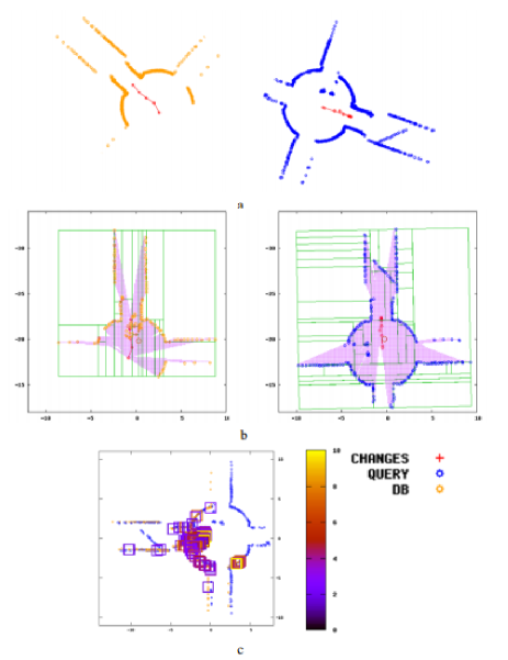
Figure 1: The key idea is viewpoint planning in which the origin of the local map coordinate (termed “viewpoint”) is planned by scene parsing and determined by our “viewpoint planner” to be invariant against small variations in self-location and changes, which aims at providing similar viewpoints for similar scenes (i.e., the relevant map pair) and enables a direct comparison of both the appearance and the pose of visual features between each map pair (i.e., without requiring pre-alignment of each map pair). (a) A query local map (left) and a database local map (right) together with the robot’s trajectory (red points). (b) Scene parsing results (green line segments) and planned viewpoint (the big red point). (c) Detected anomaly (small colored boxes) and anomaly-ness score (color bar).

I Introduction

Change detection, i.e., anomaly detection from local maps built by a mobile robot at multiple different times, is a fundamental problem in robotic mapping and localization [1], with many important applications ranging from map users (e.g., patrol robots) to mapper robots (e.g., map maintenance robots). Given a local map of a robot’s surroundings as a query, the goal of change detection is to search over a database or a collection of previously built local maps to identify regions that correspond to environment changes (e.g., appearance of new objects), which comprise the “change mask”. A key issue is that the change mask should not contain “unimportant” or “nuisance” forms of change, such as those induced by difference in views and sensor noises. In this sense, change detection is similar in its objectives to anomaly detection [2], where the goal is to detect anomalies that are interesting to the observer.

Although the change detection problem has drawn much research attention during the past decade [3, 4, 5, 6, 7], it is still a difficult problem to solve in practice. Most previous works either cannot be applied to scenarios where the size of the map collection is large [6], or simply assumed that the robot self-location is globally known [4]. For instance, in [3] and in other related papers, image-based change detection from a cadastral 3D model of a city by using panoramic images captured by a car is addressed under inaccuracies in input geometry, errors in the image’s GPS data, as well as, limited amount of information owing to sparse imagery. However, it is not straightforward to extend such approaches to the case of large-scale map collection and globally unknown self-location. The number of possible local maps that need to be examined is large and prohibitive without compressed map representation and efficient map retrieval mechanism.

In this paper, we tackle the problem of simultaneous self-localization and change detection, by reformulating the problem as a map retrieval problem, and propose a local map descriptor with a compressed bag-of-words (BoW) structure as a scalable solution (Fig. 1). We make the following contributions:

(1) To enable a direct comparison of the spatial layout of visual features between different local maps, the origin of the local map coordinate (termed “viewpoint”) is planned by scene parsing and determined by our “viewpoint planner” to be invariant against small variations in self-location and changes. This strategy is inspired by our previous work on grammar-based map parsing [8] and unique viewpoint planning [9], aiming at providing similar viewpoints for similar scenes (i.e., the relevant map pair).

(2) We extend the BoW model to enable the use of not only the appearance (e.g., polestar [10]) but also the spatial layout (e.g., spatial pyramid [11]) of visual features with respect to the planned viewpoint. The key observation is that the planned viewpoint (i.e., the origin of local map coordinate) acts as a pseudo viewpoint that is usually required by spatial BoW (e.g., SPM [11]) and also by anomaly detection (e.g., NN-d [12], LOF [13]).

(3) Experimental results on a challenging “loop-closing” scenario show that the proposed method outperforms previous BoW methods in self-localization, and furthermore that the use of both appearance and pose information in change detection produces better results than the use of either information alone. Although our approach is general and can be applicable to various sensor modalities and applications, we focus on an application scenario of 2D pointset maps from laser data [14], a challenging scenario owing to sparse sensing and limited field-of-view.

The use of spatial information in the BoW model (e.g., SPM) has been studied in the field of large-scale image retrieval [15]. However, to adopt such methods that were originally proposed for image data, we must first determine the viewpoint or the origin of the local map coordinate with respect to which poses of local features are defined, which is a non-trivial task and is our contribution in this paper.

This study is a part of our studies on long-term map learning [16] and map-matching [17], and is built on our previous techniques for BoW map retrieval [18], grammar based scene parsing [8], unique viewpoint planning [9], and change detection [19]. However, the use of spatial BoW and anomaly detection is not addressed in existing studies.

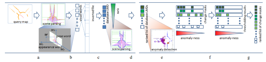
Figure 2: The overall pipeline of the algorithm, which involves four main steps: viewpoint planning (a), local map descriptor (b), global self-localization (c: database retrieval, d: SPM matching) and change detection (e: anomaly detection, f: thresholding, g: re-ranking), which are described in sections III, III-A, III-B, and III-C, respectively.

I-A Related Work

Although various types of “change detection” tasks (i.e., detecting changes from scenes taken at multiple different times, including video surveillance, remote sensing, medical diagnosis and civil infrastructure) have been studied in the literature [20], in these studies, researchers often assume the availability of global self-location information (e.g., GPS) or perfect scene registration, and then apply a simple differencing or a more sophisticated method to identify regions of changes. In contrast, our focus is on the applications of robotic mapping and localization [1], in which the self-location of the robot is globally unknown, and self-localization itself is a challenging topic of ongoing research [21].

In recent years, change detection under local uncertainty in viewpoint has also been addressed by several researchers [3, 4, 5, 6, 7]. In [5], a change detection algorithm for “difference detection” by a patrol robot was considered; however, the focus was on NDT-based scene representation and its use in change detection rather than on viewpoint’s uncertainty. In [3], “city-scale” change detection was built upon the authors’ previous work; however, the availability of rough GPS information (i.e., viewpoint) was assumed. In [6], a reliable solution to change detection from LIDAR data was addressed by introducing a method for reasoning on frontiers and occlusions; however, the focus was on uncertainty in object location rather than in viewpoint. In contrast, we do not rely on prior knowledge of viewpoint, but instead, our viewpoint planner provides an invariant viewpoint that acts as a pseudo viewpoint for change detection.

State-of-the-art map matching techniques often employ offline pre-computation of an efficient scene model to accelerate online scene retrieval [22], rather than employing just online scene matching by random sample consensus (RANSAC), iterative closest point (ICP), correlation, or other similar techniques such as Chamfer matching. Our focus, the BoW model, is one of the most established approaches for scalable scene retrieval [23]. Unlike many other map models (e.g., Hough transform) in which a scene is represented by a single global scene descriptor, the BoW model is sufficiently flexible to describe a variety of local maps with very different scales as unordered collection of local features.

Our focus, pose information of local features, is orthogonal to the type of appearance descriptors to be used. In [14], the problem of extracting salient local appearance features from a given local map is discussed. In this study, we employ several different appearance descriptors, derived from our previous studies [24] and [18]. In general, appearance and spatial information complement each other.

Our approach to anomaly detection, i.e., detecting previously unobserved patterns in data [2], belongs to the class of nearest neighbor (NN) based anomaly detection [12], as it is suitable for anomaly detection from very small samples, i.e., a sole relevant pair of query and database maps.

It should be emphasized that our map descriptor does not aim for replacing existing map representations but rather for providing complementary information. Translation from other map representations (e.g., grid, feature, or view sequence maps) [1] to our map descriptor is often straightforward, which enables efficient BoW map retrieval.

Our viewpoint planner can be viewed as a novel application of grammar-based scene parsing, which has been previously studied in the fields of point-based geometry, image description, scene reconstruction and scene compression.

II Problem

Our goal is to take a 2D pointset map as a query input, and to search over a size $N$ map database to obtain a ranked list of self-location candidates (i.e., identifying the database map of change) and change masks (i.e., anomalies with respect to the database map).

The main steps are as follows (Fig. 2). (1) As a pre-processing step, each database map is translated to a BoW map descriptor (III-A), and indexed by an inverted file system. This pre-processing step can be done as part of the map-building task. (2) Given a query local map, it is translated to a BoW descriptor and the inverted file is accessed based on the word address. This visual search process employs SPM similarity metric. As a result, we obtain a ranked list of database BoW descriptors (III-B). (3) Then, we proceed down the list, examining the retrieved database maps one by one and evaluate the anomaly-ness of each feature point from each database map (III-C), and if it exceeds a threshold then we push back the point’s change mask to a list. For the results, we obtain a ranked list of change masks.

III Approach

The core of our novel map representation, LMD, is viewpoint planning (Fig. 4), aiming at planning the origin $(x^{v},y^{v})$ of the local map coordinate, with respect to which poses of local features (or pose words) are defined.

Our approach to viewpoint planning is quite simple: determining the “center” of a given local map as its viewpoint (Fig. 1b). This strategy is motivated by an intuition that the local map’s center is expected to be more robust than such as its boundary. Our viewpoint planner first estimates the orientation of the dominant direction of the scene structure by using the entropy minimization criteria in [25], and defines the $x$-direction of the local map coordinate system to be the dominant direction. Then, it performs scene parsing by using the Manhattan world grammar in [8] to extract a set of wall primitives. Finally, it imposes a grid map with an $xy$ resolution of 0.1 m and assigns each cell “occupied” (i.e., wall cells), “unoccupied”, or “unknown” label [1].

The remaining problem is how to determine the center of a given local map. Considering that a key requirement is providing similar viewpoints (i.e., “center”) for similar scenes (i.e., the relevant map pair) under small variations in self-location and changes, we propose two strategies. One strategy is to define the viewpoint as the center of gravity (CoG) of wall cells. Another strategy is the so-called center of rooms (CoR), which analyzes not the wall primitives but the structure of rooms. More formally, we analyze the rectangular regions of unoccupied cells termed “rooms” aligned with the orthogonal directions of the quasi-Manhattan world (Fig. 4). We then densely sample rooms and then define the viewpoint as the center of gravity of “dominant” room cells. For robustness, we generate two histograms of $f^{x}(x)$ and $f^{y}(y)$ of room cells along two dominant directions $x,y$ and consider only those dominant cells $(x,y)$ where the histogram values $f^{x}(x),f^{y}(y)$ both exceed $90\%$ of the peak values $\max_{x}f^{x}(x)$, $\max_{y}f^{y}(y)$.

Once viewpoint is planned, it is straightforward to adopt existing techniques for spatial BoW (e.g., SPM) and anomaly detection (e.g., LOF, NN-d), as explained below.

III-A Local Map Descriptor

Once the viewpoint is determined, computation of the BoW vector is straightforward. We compute the local appearance feature descriptors (e.g., polestar, shape context, etc.) of local features as well as their poses with respect to the planned viewpoint, and then quantize them to a pose word $(w_{x},w_{y})$ and an appearance word $w_{a}$. For the result, we obtain word vectors, each having the form:

$$X=\{\langle w_{a},w_{x},w_{y}\rangle\}.$$ (1)

We employ an appearance descriptor that is similar in concept to shape context [26] or polestar [27], which proved successful in our previous work on map matching [24][18]. First, a circular interest region with radius $R$ [m] is placed at each interest point, and then, the interest region is decomposed into 10 concentric shells with radius $r_{i}$ $(i\in[1,10])$ and $A$ sectors as $a_{j}$ $(j\in[1,A])$ that emerged from the interest point. To compute an appearance descriptor, we employ a temporary grid map with spatial resolution 0.01 m.

Each descriptor is mapped to a $B=10$ bit code termed visual word by using a random projection matrix derived from our previous work in [28]. This dimension reduction consists of two steps: (1) The input $D$-dim descriptor is mapped by a pre-defined $B\times D$ random projection matrix to obtain $B$-dim short vector; (2) Each element of a $B$-dim short vector is binarized based on its sign and then the binary vector is encoded to a $B$-bit visual word.

III-B Global Self-localization

The global self-localization step (i.e., identifying the database map of change) follows the SPM framework [11], by placing a sequence of increasingly coarser grids over the local map and taking a weighted sum of the number of matches that occur at each level of resolution. Although the area of a map is variable, we use three different levels $l=0,1,2$ of resolutions $W2^{-l}$[m] for a fixed width $W=5$.

Following the pyramid match kernel [11], at any resolution $l$, the two BoW vectors are compared and similarity $I^{l}$ between a pair of BoW vectors is measured in terms of the number of matched visual words. The map level similarity $K$ between a pair of LMDs $X$ and $X^{\prime}$ is defined as:

$$K(X,X^{\prime})=\frac{1}{2^{L}}I^{0}+\sum_{l=1}^{L}\frac{1}{2^{L-l+1}}I^{l}.$$ (2)

We hypothesize and test four different orientations $(\pi/2)i$ $(i=0,1,2,3)$ between each pair of quasi-Manhattan aligned query and database maps, and use the best hypothesis with the highest similarity score $K$.

Note that each relevant map pair found by the above global self-localization is used as input and will be compared by the next change detection step (Fig.2). To accelerate change detection, we propose to use the global self-localization step to provide a fine alignment of map pairs to address the estimation errors of the planned viewpoint. We compute the mode of a histogram of differences of pose words

$$\Delta x=w_{x}^{query}-w_{x}^{DB};~{}~{}~{}\Delta y=w_{y}^{query}-w_{y}^{DB}$$ (3)

and use the mode as a temporary offset for the pose words of the database local map during the change detection step.

III-C Change Detection

Given feature locations with respect to the planned viewpoint, our anomaly detection step follows NN based anomaly detection approaches (LOF, NN-d). It has two steps:

First, we evaluate LOF [13] to identify and eliminate outlier features, such as occlusions and noises, which should not contribute to change detection. Given a set of feature points, LOF estimates outlier-ness, which is the degree of each point being an outlier. Let $D^{lrd}(p)$ denote the local reachability density of point $p$

$$D^{lrd}(p)=\frac{1}{|S^{NN}(p)|}\sum_{o\in S^{NN}(p)}D^{reach}(p,o),$$ (4)

where $S^{NN}(p)$ is the $K$-NN of a given point $p$ and $D^{reach}$ is the reachability distance, which can be seen as an extension of the point distance function to have a smoothness effect as defined in [13]. Then, LOF is evaluated by

$$D^{lof}(p)=\frac{1}{|S^{NN}(p)|}\sum_{o\in S^{NN}(p)}\left[D^{lrd}(o)/D^{lrd}(p)\right].$$ (5)

We use a fixed threshold value $T^{lof}=1.6$ [13] and a point $p$ is regarded as an outlier if $D^{lof}(p)$ exceeds $T^{lof}$.

Second, we evaluate NN-d [12] to detect changes from appearance words in a query map by using the appearance words in the database map as training data. A 60-dim appearance descriptor (III-A) is extracted for each “non-outlier” feature point with a parameter setting of $(R,A)=(6,10)$, and then each element of the vector is binarized using the average of all the 60 elements as a threshold, which yields a 60-bit string as an appearance word for change detection. Dissimilarity between a pair of appearance words is evaluated by Hamming distance. The output of NN-d is an indication of the validity of the object and

$$r(p)=|S^{NN}(p)-p|_{2}\Big{[}|S^{NN}(p)-S^{NN}(S^{NN}(p))|_{2}\Big{]}^{-1}.$$ (6)

We use both the appearance and pose information of visual features for anomaly detection. We employ the $K=1$ nearest neighbor version of NN-d [12] and thus $S^{NN}(p)$ is the 1-NN of a given point $p$, and we search the 1-NN within a fixed size window $=[-3,3]$[m]$\times$$[-3,3]$[m] centered at a prediction of the query feature’s location, which is simply predicted from the planned viewpoint $p^{v}$ and the original query feature’s location with respect to the query local map’s coordinate. We first threshold feature points $p_{i}$ by a threshold $r(p_{i})>T^{NN-d}$ (e.g., $T^{NN-d}=1.5$) and then rank the surviving feature points in descending order of the map level similarity $K$ in (2).

Note that in our scenario, the original high dimensional appearance feature vectors are no longer available as they are encoded and replaced using a compact BoW model with 60-bit appearance words. Of course, this approximation causes quantization loss. However, combining pose and appearance words are often sufficient to obtain accurate results, as we will see in the next experimental section.

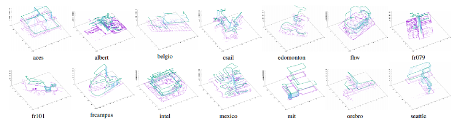
Figure 3: Datasets. (Purple points: point clouds. Green curve: robot’s trajectory. Each of the light blue line segments connects a local map pair that corresponds to each ground-truth loop closing.)

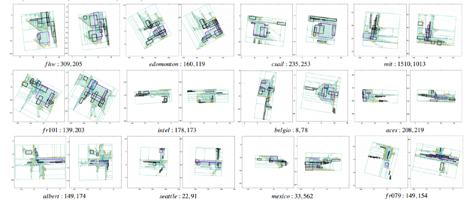
Figure 4: Samples of scene parsing. 12 ($=3\times 4$) different pairs of scene parsing are shown for 12 relevant pairings of a query local map (left) and a relevant database local map (right) with “query map’s ID, database map’s ID”. (Orange points: datapoints from the original local map. Boxes: “room” primitives proposed by the CoR method. The green big circle: planned viewpoint. Small blue points with lines: the robot’s trajectory. Green dots: unoccupied cells.)

IV Experiments

We conducted change retrieval experiments to verify the efficacy of the compressed LMD approach. In the following subsections, we first describe the datasets and investigate the influence of parameter settings and then report the experimental results on self-localization and change detection.

IV-A Settings

We created a large-size map collection from a dataset that was kindly provided by researchers online , which comprises odometry and laser data logs acquired by a car-like mobile robot in indoor environments (Fig. 3). The datasets were scan matched to obtain pointset maps from each of 14 datasets “aces”, “albert”, “belgio”, “csail”, “edomonton”, “fhw”, “fr079”, “fr101”, “frcampus”, “intel”, “mexico”, “mit”, “orebro”, “seattle” that were obtained from the long travel of the mobile robot, each of which corresponded to 240-4,800 scans. In the current experiments, each local map corresponds to a 5 m run of the robot, and a new local map is initialized every time the robot runs 1 m along the trajectory, yielding around 80-640 occupied cells per map.

For each query map, we simulated the appearance of new objects that were not observed in the database map. Our change simulator places a change region with size $w[m]\times h[m]$ $(w,h\in[1.0,2.0])$ at random location and generates a set of small virtual rectangular objects within the changed region. We then run a ray tracing algorithm to obtain modified datapoints that reflect changed objects. If a ray hits such a virtual changed object, the corresponding laser range measurement is replaced by the virtual measurement originated from the virtual object. If any ray does not hit any virtual object, it is impossible to detect such a change and thus we re-run the change simulator. However, note that our recognition algorithm does not assume any prior knowledge about the shape, pose, and size of the environment changes.

We consider a challenging scenario of self-localization, called loop closing [1], in which a robot traverses a loop-like trajectory and then returns to the previously explored location. More formally, the relevant map pair is defined by a database map that satisfies two conditions (light blue lines in Fig. 3): 1) The average distance of the datapoints from each query datapoint to their nearest neighbor database datapoint is nearer than other candidates. 2) Its distance traveled along the robot’s trajectory is sufficiently distant ($>10$ m) from that of the query map. As a result, a relevant pair of maps become dissimilar to each other, which makes our self-localization and change detection tasks a challenging one.

For each of the 14 datasets, we uniformly sampled 10 different queries and conducted $10\times 14$ $=140$ change detection tasks. This required a comparison of 12,320 pairs of query and database maps in total.

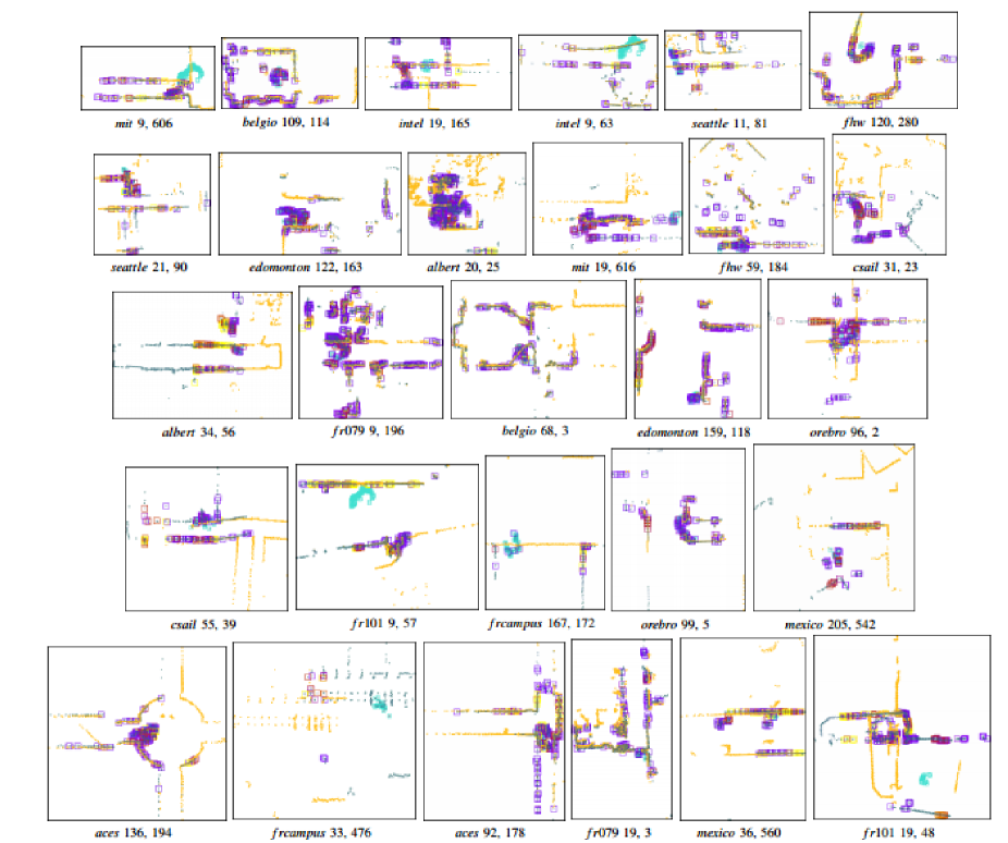
Figure 5: Change detection. Point clouds of the query and relevant database maps and ground-truth changes (light blue points) are overlaid using the information of the planned viewpoint, and are shown with “query map’s ID, database map’s ID”. The meaning of the datapoints, anomalies, and anomaly-ness is the same as in Fig.1.

IV-B Viewpoint Planning

Fig. 4 shows several examples of viewpoint planning using the CoR method in III-A. Results from each step of the CoR method, (1) entropy based orientation estimation, (2) scene parsing by Manhattan world grammar, (3) sampling of room primitives, and (4) determining of viewpoint are shown in the figure. One can see that our planner frequently provides similar viewpoints for the relevant map pair, even when the robot’s trajectories are very different between the map pair.

IV-C Change Detection

Fig. 5 shows several examples of change detection tasks. Here, we used the default value of the threshold on anomaly-ness $T^{NN-d}=1.5$. The figure shows change detection of 28 pairs uniformly sampled from the 140 relevant pairs. It can be seen that change detection was successful in most of the examples shown here. Exceptionally, change detection failed for the cases of “intel 9, 63”, “fr101 9, 57”, “frcampus 33, 476”, and “fr101 19, 48”. In “intel 9, 63” and “fr101 9, 57”, the change regions were near the static large walls; thus the robot could not distinguish the changes from the known walls. In “frcampus 33, 476”, one can see that self-localization was not successful owing to errors in viewpoint planning, and as a result, the robot could not discriminate changes from known objects. In “fr101 19, 48”, the robot failed to select the correct viewpoint orientation (among the four candidates explained in III-B), owing to unknown objects caused by changes, and in consequence, it failed to detect the changes. For the other 24 examples, change detection was successful by using both appearance and pose information from our LMD descriptor.

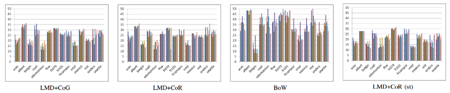
Figure 6: Self-localization performance. (Vertical axis: ANR[%]. For each dataset, from left to right, results for descriptor #1, …, #8 are shown. )

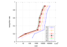
$mit$

$belgio$

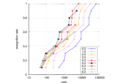
$intel$

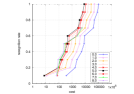
$fhw$

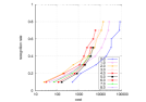
$frcampus$

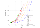
$mexico$

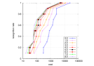
$seattle$

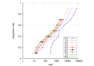
$edomonton$

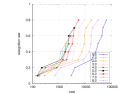
$albert$

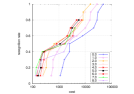
$csail$

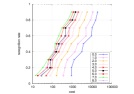
$orebro$

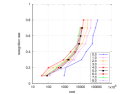
$fr101$

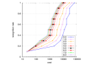
$aces$

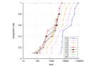
$fr079$

Figure 7: Change detection performance (LMD+CoG, descriptor#1). Horizontal axis: rank of change mask (log-scale). Vertical axis: recognition rate.

IV-D Performance of Global Self-localization

This subsection investigates the performance of global self-localization. For the performance evaluation, we used the averaged normalized rank (ANR) [29] as a performance index. ANR is a ranking-based performance measure in which a lower value is better. To determine the ANR, we performed a number of $N$ independent self-localization tasks with various queries and databases. For each task, the rank assigned to the ground-truth database map by a self-localization method of interest was investigated, and the rank was normalized by the database size $N$. The ANR was subsequently obtained as the average of the normalized ranks over all the self-localization tasks. These self-localization tasks were conducted using 2,896 different queries and a size 6,193 map database in total.

Self-localization performance is also measured by its recognition rate. Given a query local map, its retrieval result is in the form of a ranked list of database maps. Then, the recognition rate $y$ is defined over a set of self-localization tasks, as the ratio $y$ of tasks whose relevant database maps are correctly included in the top $x$ ranked maps.

TABLE I: Top-$X$% recognition rate for 2,590 retrieval expewriments

map retrieval method	Top-10		Top-5
LMD+CoG	0.44	( 1141 )	0.36	( 930 )
LMD+CoR	0.45	( 1157 )	0.35	( 908 )
BoW	0.25	( 645 )	0.15	( 396 )
LMD+CoR (st)	0.54	( 1393 )	0.45	( 1161 )

Fig. 6 and Table I (“LMD+CoG”, “LMD+CoR”) report the results. It can be seen that the proposed LMD method (LMD+CoG, LMD+CoR) produces good ANR performance (15%-30%) for most datasets considered here.

IV-E Influence of Appearance Descriptors

We also tested eight different appearance feature descriptors (III-A) with different parameter settings of $(R,A)$: $(1,1)$, $(6,3)$, $(12,6)$, $(1,6)$, $(3,6)$, $(6,6)$, $(3,1)$, and $(6,1)$. The descriptors #1, #7 and #8 can be viewed as variants of rotation invariant polestar descriptors [27], whereas the other ones can be viewed as variants of the shape context [26], both of which were successful in our previous work on map matching [18, 24]. We tested all the eight descriptors for all the datasets. For the result, the ANR per query was 25.8, 25.1, 24.6, 25.6, 25.1, 24.7, 25.1, and 25.5, and the ANR per dataset was 26.1, 26.3, 26.2, 28.7, 26.3, 26.8, 25.6, and 26.5 for each descriptor #1, …, #8. It can be said the performance difference between the descriptors was not significant in the current experiments. For the sake of simplicity, we employed descriptor #1 (polestar descriptor) in the following experiments.

IV-F Comparison against the BoW Method

To demonstrate the efficacy of the proposed LMD approach, using spatial information in the BoW model, we also compared the performance of the proposed LMD method against the previous BoW method that does not use spatial information, which is shown in Fig. 6 and Table I (“BoW”). As expected, the performance of the BoW method was significantly lower. In contrast to that, our method performed well as our method could exploit not only the appearance but also the poses of features to discriminate stationary objects (i.e., landmarks) from changes.

IV-G Comparison with Stationary Environments

We also tested the proposed CoR method in an alternative scenario of stationary environments, i.e., without the appearance of new objects. Fig. 6 and Table I (“LMD+CoR (st)”) show the results, where the performance is much better than in the case of non-stationary environment, (“LMD+CoR”). This results demonstrate the difficulty of self-localization in non-stationary environments addressed in this study.

IV-H Performance of Change Detection

Fig. 7 reports the performance of change detection. To investigate the efficacy of NN-d anomaly detection, we compared different settings of the threshold on anomaly-ness $T^{NN-d}$: 0.0, 1.0, … and 8.0. As mentioned, feature points were first thresholded and then ranked in descending order of map level similarity $K$, provided by the self-localization step. When anomaly-ness was ignored (e.g., $T^{NN-d}=0.0$), a huge amount of false-positive “changes” were detected. When threshold $T^{NN-d}$ was too high (e.g., $T^{NN-d}=7.0,8.0$), many changes were missed. In consequence, medium threshold values $T^{NN-d}=1.0,2.0,3.0$ yielded a good balance between cost and performance. It can be said that the use of not only pose but also appearance information, provided by the proposed LMD descriptor is important for a successful self-localization and change detection.

V Conclusion and Future Work

In this study, we tackled and reformulated the problem of simultaneous self-localization (i.e., identifying the database map of change) and change detection (i.e., identifying anomalies with respect to the database map) as a map retrieval problem, and proposed a local map descriptor with a compressed bag-of-words (BoW) structure as a scalable solution. As a primary novelty, the origin (or the viewpoint) of the local map coordinate is planned by scene parsing and determined by our “viewpoint planner” to be invariant against small variations in self-location and changes, aiming at providing similar viewpoints for similar scenes (i.e., the relevant map pair). We also extended the BoW model to enable the use of not only the appearance but also the pose of visual features with respect to the planned viewpoint. The key observation was that the planned viewpoint (i.e., the origin of local map coordinate) acts as a pseudo viewpoint that is usually required by spatial BoW (e.g., SPM) and also by anomaly detection (e.g., NN-d, LOF). Experiments on a challenging loop-closing scenario showed that the proposed LMD method outperformed the previous BoW method in self-localization and furthermore that the use of both appearance and pose information in change detection produces better results than the use of either information alone.

Our work is the first significant attempt in tapping into compressive change retrieval. While it shows promises, the problem is far from solved. In this study, our experiments were restricted to the 2D environment maps with 3 dof viewpoint planning. An immediate future step is to apply our algorithm on 3D pointset maps with 6 dof viewpoint planning, such as from 3D LIDAR data. Another future direction is to explore different appearance features. In this work, we focused on shape features that are effective in pointset maps, but there are many other types of appearance features such as color features and texture features [16]. In addition, we implemented a scene parsing algorithm using a Manhattan world grammar. One challenging extension is to analyze scene structure in more general scenarios of unstructured environments [29].

References

- [1] S. Thrun, W. Burgard, and D. Fox, Probabilistic robotics. MIT press, 2005.
- [2] V. Chandola, A. Banerjee, and V. Kumar, “Anomaly detection: A survey,” ACM computing surveys (CSUR), vol. 41, no. 3, p. 15, 2009.
- [3] A. Taneja, L. Ballan, and M. Pollefeys, “City-scale change detection in cadastral 3d models using images,” in IEEE CVPR, 2013.
- [4] ——, “Geometric change detection in urban environments using images,” IEEE T. PAMI, vol. 37, no. 11, pp. 2193–2206, 2015.
- [5] H. Andreasson, M. Magnusson, and A. Lilienthal, “Has somethong changed here? autonomous difference detection for security patrol robots,” in IEEE/RSJ IROS, 2007, pp. 3429–3435.
- [6] P. Drews, S. da Silva Filho, L. Marcolino, and P. Nunez, “Fast and adaptive 3d change detection algorithm for autonomous robots based on gaussian mixture models,” in IEEE ICRA, 2013, pp. 4685–4690.
- [7] P. Neubert, N. Sünderhauf, and P. Protzel, “Superpixel-based appearance change prediction for long-term navigation across seasons,” Robotics and Autonomous Systems, vol. 69, pp. 15–27, 2015.
- [8] K. Kondo, K. Tanaka, and T. Nagasaka, “Grammar-based map compression using manhattan world priors,” in IEEE ROBIO, 2011.
- [9] S. Hanada and K. Tanaka, “M2t: Local map descriptor,” in IEEE/SICE SII, 2014, pp. 210–215.
- [10] E. Silani and M. Lovera, “Star identification algorithms: Novel approach & comparison study,” IEEE T. aerospace and electronic systems, vol. 42, no. 4, pp. 1275–1288, 2006.
- [11] S. Lazebnik, C. Schmid, and J. Ponce, “Beyond bags of features: Spatial pyramid matching for recognizing natural scene categories,” in IEEE CVPR, vol. 2, 2006, pp. 2169 – 2178.
- [12] D. M. J. Tax, One-class classification. TU Delft, Delft University of Technology, 2001.
- [13] M. M. Breunig, H.-P. Kriegel, R. T. Ng, and J. Sander, “Lof: identifying density-based local outliers,” in ACM sigmod record, vol. 29, no. 2. ACM, 2000, pp. 93–104.
- [14] G. D. Tipaldi and K. O. Arras, “Flirt-interest regions for 2d range data,” in IEEE ICRA, 2010, pp. 3616–3622.
- [15] S. J. and Z. A., “Video google: a text retrieval approach to object matching in videos,” IEEE ICCV, pp. 1470–1477, 2003.
- [16] A. Masatoshi, C. Yuuto, T. Kanji, and Y. Kentaro, “Leveraging image-based prior in cross-season place recognition,” in ICRA, 2015.
- [17] K. Tanaka and E. Kondo, “Incremental ransac for online vehicle relocation in large dynamic environments,” in IEEE ICRA, 2006.
- [18] K. Tanaka and K. Kondo, “Multi-scale bag-of-features for scalable map retrieval.” JACIII, vol. 16, no. 7, pp. 793–799, 2012.
- [19] H. Zha, K. Tanaka, and T. Hasegawa, “Detecting changes in a dynamic environment for updating its maps by using a mobile robot,” in IEEE/RSJ IROS, vol. 3, 1997, pp. 1729–1734.
- [20] R. J. Radke, S. Andra, O. Al-Kofahi, and B. Roysam, “Image change detection algorithms: a systematic survey,” Image Processing, IEEE Transactions on, vol. 14, no. 3, pp. 294–307, 2005.
- [21] S. M. Lowry, N. Sünderhauf, P. Newman, J. J. Leonard, D. D. Cox, P. I. Corke, and M. J. Milford, “Visual place recognition: A survey,” IEEE TRO, vol. 32, no. 1, pp. 1–19, 2016.
- [22] E. Olson, “M3RSM: many-to-many multi-resolution scan matching,” in IEEE ICRA, 2015, pp. 5815–5821.
- [23] R. Arandjelović and A. Zisserman, “Three things everyone should know to improve object retrieval,” in IEEE CVPR, 2012.
- [24] K. Saeki, K. Tanaka, and T. Ueda, “Lsh-ransac: An incremental scheme for scalable localization,” IEEE ICRA, pp. 3523–3530, 2009.
- [25] S. Olufs and M. Vincze, “Robust single view room structure segmentation in manhattan-like environments from stereo vision,” in IEEE ICRA. IEEE, 2011, pp. 5315–5322.
- [26] M. G., B. S., and M. J., “Shape contexts enable efficient retrieval of similar shapes,” IEEE CVPR, pp. 723–730, 2001.
- [27] E. Silani and M. Lovera, “Star identification algorithms: Novel approach & comparison study,” IEEE Trans. Aerospace and Electronic Systems, vol. 42, no. 4, pp. 1275–1288, 2006.
- [28] T. Nagasaka and K. Tanaka, “An incremental scheme for dictionary-based compressive slam,” IEEE/RSJ IROS, 2011.
- [29] S. Hanada and K. Tanaka, “Partslam: Unsupervised part-based scene modeling for fast succinct map matching,” in IEEE/RSJ IROS, 2013.