Of Genes and Machines: application of a combination of machine learning tools to astronomy datasets

Abstract

We apply a combination of a Genetic Algorithms (GA) and Support Vector Machines (SVM) machine learning algorithm to solve two important problems faced by the astronomical community: star/galaxy separation, and photometric redshift estimation of galaxies in survey catalogs. We use the GA to select the relevant features in the first step, followed by optimization of SVM parameters in the second step to obtain an optimal set of parameters to classify or regress, in process of which we avoid over-fitting. We apply our method to star/galaxy separation in Pan-STARRS1 data. We show that our method correctly classifies 98% of objects down to $i_{\rm P1}=24.5$, with a completeness (or true positive rate) of 99% for galaxies, and 88% for stars. By combining colors with morphology, our star/classification method yields better results than the new SExtractor classifier spread_model in particular at the faint end ($i_{\rm P1}>22$). We also use our method to derive photometric redshifts for galaxies in the COSMOS bright multi-wavelength dataset down to an error in $(1+z)$ of $\sigma=0.013$, which compares well with estimates from SED fitting on the same data ($\sigma=0.007$) while making a significantly smaller number of assumptions.

1. Introduction

Astronomy has witnessed an ever-increasing deluge of data over the past decade. Future surveys will gather very large amounts of data daily that will require on-the-fly analysis to limit the amount of data that can be stored or analyzed, and allow timely discoveries of candidates to be followed-up: for instance Euclid (Laureijs et al., 2011, 100 GB per day), WFIRST (Spergel et al., 2015, 1.3TB per day), or the Large Synoptic Survey Telescope (LSST, Ivezic et al., 2008, 10 TB per day). The evolution of the type, volume, cadence of the astronomical data requires the advent of robust methods that will enable a maximal rate of extraction of information from the data. This means that for a given problem, one needs to make sure all the relevant information has is made available in the first step, followed by the use of a suitable method that is able to narrow down on the important aspects of the data. This can be both for feature selection as well as for noise filtering.

In machine learning parlance, the tasks required can be designated as classification tasks (derive a discrete value: star vs galaxy for instance) or regression tasks (derive a continuous value: photometric redshift for instance.) Methods for classification or regression usually are of two kinds: physically motivated, or empirical. Physically motivated methods use templates built from previously observed data, like star or galaxy Spectral Energy Distributions (SEDs) for instance in the case of determining photometric redshifts. They also attempt at including as much knowledge as we have of the processes involved in the problem at stake, such as prior information. Physically motivated methods seem more appropriate than empirical, however the very fact that they require a good knowledge of the physics involved might be a important limitation. Indeed, our knowledge of a number of processes involved in shaping the SEDs of galaxies for instance is still quite limited (e.g. Conroy et al., 2010, and references therein): whether is it about the processes driving star formation, dust attenuation laws, initial mass function, star formation history, AGN contribution etc …Hence choices need to be made: either make a number of assumptions, in order to reduce the number of free parameters. Or, one can decide to be more inclusive and add more parameters, but at the cost of potential degeneracies. Physically motivated methods are also usually limited in the way they treat the correlation between the properties of the objects, because the only correlations taken into account are those included in the models used, and might not reflect all of the information contained in the data.

On the other hand, empirical methods require few or no assumptions about the physics of the problem. The goal of an empirical method is to build a decision function from the data themselves. The quality of the generalization of the results to a full dataset depends of course on the representativity of the training sample. We note however that the question of the generalization also applies to physically motivated methods, as they are also validated on the training data.

Depending on the methods used, transformations may need to be effected before the method is applied; for example in the case of Support Vector Machines (SVM, e.g. Boser et al., 1992; Cortes & Vapnik, 1995; Vapnik, 1995; Smola & Schölkopf, 1998; Vapnik, 1998; Duda et al., 2001) linear separability is presumed, thereby requiring non-linearly separable or regressible data to be kernel transformed to enable this.

A challenge with empirical methods is that with growing numbers of input parameters, it becomes prohibitive in terms of CPU time to use all of them. It can also be counter-productive to feed the machine learning tool with all of these parameters, as some of them might either be too noisy, or not bring any relevant information to the specific problem to tackle. Moreover, high dimensional problems suffer from the bane of being over fit by machine learning methods (Cawley & Talbot, 2010), thereby yielding high-dimensional non-optimal solutions. This requires sub-selection of relevant variables from a large $N-$dimensional space (with $N$ potentially close to 1000). This task itself can also be achieved using machine learning tools. Here we present, to our knowledge, the first application to astronomy of the combination of two machine learning techniques: Genetic Algorithms (GA, e.g. Steeb, 2014) for selecting relevant features followed by SVM to build a decision/reward function. GA alone have already been used in astronomy for instance to study the orbits of exoplanets, and the SEDs of young stellar objects (Cantó et al., 2009), the analysis of SNIa data (Nesseris, 2011), the study of star formation and metal enrichment histories of resolved stellar system (Small et al., 2013), the detection of globular clusters from HST imaging (Cavuoti et al., 2014), or photometric redshifts estimation (Hogan et al., 2015). On the other hand, SVM have been extensively used to solve a number of problems such as object classification (Zhang & Zhao, 2004), the identification of red variables sources (Woźniak et al., 2004), photometric redshift estimation (Wadadekar, 2005), morphological classification (Huertas-Company et al., 2011), and parameters estimation for Gaia spectrophotometry (Liu et al., 2012). We note also that the combination of GA and SVM has already been used in a number of fields such as cancer classification (e.g. Huerta et al., 2006; Alba et al., 2007), chemistry (e.g. Fatemi & Gharaghani, 2007), bankruptcy prediction (e.g. Min et al., 2006) etc …We do not attempt here to provide the most optimized results from this combination of methods. Rather, we present a proof-of-concept that shows that GA and SVM yield remarkable results when combined together as opposed to using the SVM as a standalone tool.

In this paper, we focus on two tasks frequently seen in large surveys: star/galaxy separation and determination of photometric redshifts of distant galaxies. Star/galaxy separation is a classification problem that has been usually constrained purely from the morphology of the objects (e.g. Kron, 1980; Bertin & Arnouts, 1996; Stoughton et al., 2002). On the other hand, a number of studies used the color information with template fitting to separate stars from galaxies (e.g. Fadely et al., 2012). On top of these two common approaches, good results have been obtained by feeding morphology and colors to machine learning techniques (e.g. Vasconcellos et al., 2011; Saglia et al., 2012; Kovács & Szapudi, 2015). Our goal here is to extend the star/galaxy separation to faint magnitudes where morphology is not as reliable. We apply here the combination of GA with SVM to star/galaxy separation in the Pan-STARRS1 (PS1) Medium Deep survey (Kaiser et al., 2010; Tonry et al., 2012; Rest et al., 2014).

On the other hand, determining photometric redshifts is a well-studied problem of regression that has been dealt with using a variety of methods, including template fitting (e.g. Arnouts et al., 1999; Benítez, 2000; Brammer et al., 2008; Ilbert et al., 2009), cross correlation functions (Rahman et al., 2015), Random Forests (Carliles et al., 2010), Neural Networks (Collister et al., 2007), polynomial fitting (Connolly et al., 1995), symbolic regression (Krone-Martins et al., 2014). We apply the GA-SVM to the zCOSMOS bright sample (Lilly et al., 2007).

The outline of this paper is as follows. In Sect. 2 we present the data we apply our methods to, and also the training sets we use: PS1, and zCOSMOS bright. In Sect. 3 we briefly describe our methods; we include a more detailed description of SVM in an Appendix. We present our results in Sect. 4, and finally list our conclusions.

2. Data

We perform star/galaxy separation in PS1 Medium Deep data (see Sect. 2.1), using a training set built from COSMOS ACS imaging (see Sect. 2.2.1). We then derive photometric redshifts for the zCOSMOS bright sample (see Sect. 2.2.2).

2.1. Pan-STARRS1 data

The Pan-STARRS1 survey (Kaiser et al., 2010) surveyed 3/4 of the northern hemisphere ($\delta>-30$ deg), in 5 filters: $g_{\rm P1}$, $r_{\rm P1}$, $i_{\rm P1}$, $z_{\rm P1}$, and $y_{\rm P1}$ (Tonry et al., 2012). In addition, PS1 has obtained deeper imaging in 10 fields (amounting to 80 deg²) called as the Medium Deep Survey (Tonry et al., 2012; Rest et al., 2014). We use here data in the MD04 field, which overlaps the COSMOS survey (Scoville et al., 2007).

We use our own reduction of the PS1 data in the Medium Deep Survey. We use the image stacks generated by the Image Processing Pipeline (Magnier, 2006), and also the CFHT $u$ band data obtained by E. Magnier as follow up of the Medium Deep fields. We have at hand 6 bands: $u_{\rm CFHT}$, $g_{\rm P1}$, $r_{\rm P1}$, $i_{\rm P1}$, $z_{\rm P1}$, and $y_{\rm P1}$. We perform photometry using the following steps; we consider the PS1 skycell as the smallest entity: i) resample (using SWarp, Bertin et al., 2002) the u band images to the PS1 resolution, and register all images; ii) for each band fit the PSF to a Moffat function, and match that PSF to the worse PSF in each skycell; iii) using these PSF-matched images, we derive a $\chi^{2}$ image (Szalay et al., 1999); iv) we perform photometry using the SExtractor dual mode (Bertin & Arnouts, 1996), detecting objects in the $\chi^{2}$ image and measuring the fluxes in the PSF matched images: the Kron-like apertures are defined from the $\chi^{2}$ image and hence are the same over all bands ; v) for each detection we measure spread_model in each band on the original, non PSF-matched images. We consider here Kron magnitudes, which are designed to contain $\sim 90\%$ of the source light, regardless of being a point source star or an extended galaxy.

spread_model (Soumagnac et al., 2013) is a discriminant between the local PSF, measured with PSFEx (Bertin, 2011) and a circular exponential model of scale length $FWHM/16$ convolved with that PSF. This discriminant has been shown to perform better than SExtractor previous morphological classifier, class_star.

2.2. COSMOS data

2.2.1 Star/galaxy classification training set

We use the star/galaxy classification from Leauthaud et al. (2007) derived from high spatial resolution Hubble Space Telescope (HST) imaging (in the $F814W$ band) as our training set for star/galaxy classification. They separate stars from galaxy based on their SExtractor mag_auto and mu_max (peak surface brightness above surface level). By comparing the derived stellar counts with the models of Robin et al. (2007), Leauthaud et al. (2007) showed that the stellar counts are in excellent agreement with the models for $20<F814W<25$. We perform here star/galaxy separation down to $i_{\rm P1}=24.5$.

2.2.2 Spectroscopic redshift training set

We use data taken as part of the COSMOS survey (Scoville et al., 2007). We focus here on objects with spectroscopic redshifts obtained during the zCOSMOS bright campaign (Lilly et al., 2007, $i<22.5$). We use the photometry obtained in 25 bands by various groups in broad optical and near-infrared bands: Capak et al. (2007, $u^{*}$,$B_{J}$,$V_{J}$,$g^{+}$, $r^{+}$, $i^{+}$,$z^{+}$,$K_{s}$); narrow bands: Taniguchi et al. (2007, $NB816$) and Ilbert et al. (2009, $NB711$); intermediate bands Ilbert et al. (2009, $IA427$, $IA464$, $IA505$, $IA574$, $IA709$, $IA827$, $IA484$, $IA527$, $IA624$, $IA679$, $IA738$, $IA767$). We also use IRAC1 and IRAC2 photometry (Sanders et al., 2007). We consider here only objects with good redshift determination (confidence class: 3.5 and 4.5),$z<1.5$ (which yields 5,807 objects) and measured magnitudes for all the bands listed above, which finally leaves us with 5093 objects. We do not use objects with other confidence class values, as the spectroscopic redshifts can be erroneous in at least 15% of cases (Ilbert, Private communication).

3. Methods

We present here the two machine learning methods we use in this work: Genetic Algorithms are used to select the relevant features, and Support Vector Machines are used to predict the property of interest using these features.

3.1. Genetic Algorithms

Genetic algorithms (GA, e.g. Steeb, 2014) apply the basic premise of genetics to the evolution of solution sets of a problem, until they reach optimality. The definition of optimality itself is debateable, however, the general idea is to use a reward function to direct the evolution. That is, we evolve solution sets of parameters (or genes) known as organisms through several generations, according to some pre-defined evolutionary reward function. The reward function may be a goodness of fit, or a function thereof that may take into account more than just the goodness of fit. For example, one may choose to determine subsets of parameters which optimize $\chi^{2}$ or likelihood, Akaike Information criteria, energy functions, entropy, etc. The lengths of the first generation of organisms is chosen to range from the minimum expected dimensionality of the parameter space (which can be 1) to the maximum expected dimensionality of the covariance.

The fittest organisms in a particular generation are then given higher probabilities of being chosen to be the parents for successive generations using a roulette selection method based on their fitnesses. Parents are then cross-bred using a customized procedure - in our method we first choose the lengths of the children to be based on a tapered distribution where the taper depends on the fitnesses of the parents. That way the length of the child is closer to that of the fitter parent. The child is then populated using the genes of both parents, where genes that are present in both parents are given twice the weight as genes that are only present in one parent. The idea is that the child should, with a greater probability, contain genes that are present in both parents as opposed to the ones contained in only one of them. This process iteratively produces fitter children in successive generations and is terminated when no further improvement in the average organism quality is seen. Like in biological genetics, we also introduce a mutation in the genes with constant probability. The genes which are chosen to be mutated, are replaced with any of the genes that are not part of either parent, with uniform probability of choosing from the remaining genes. This allows for genes that are not part of the current gene pool to be expressed. The conceptual simplicity of genetic algorithms combined with their evolutionary analogy as applied to some of the hardest multi-parameter global optimization problems makes them highly sought after.

3.2. Support Vector Machines

Support vector machines (SVM) (e.g. Boser et al., 1992; Cortes & Vapnik, 1995; Vapnik, 1995; Smola & Schölkopf, 1998; Vapnik, 1998; Duda et al., 2001) is a machine learning algorithm that constructs a maximum margin hyperplane to separate linearly separable patterns. SVM is especially efficient in high dimensional parameter spaces,where separating two classes of objects is a hard problem, and performs with best case complexity $\mathcal{O}n_{parameters}n^{2}_{samples}$. Where the data is not linearly separable, a kernel transformation can be applied to map the original parameter space to a higher dimensional feature space where the data becomes linearly separable. For both problems we attempt to solve in this paper, we use a Gaussian Radial Basis Function kernel, defined as

$$K(x,x^{\prime})=\exp(-\gamma||x-x^{\prime}||^{2})$$ (1)

Another advantage of using SVM is that there are established guarantees of their performance which has been well documented in literature. Also, the final classification plane is not affected by local minima in the classification or regression statistic, which other methods based on least squares, or maximum likelihood may not guarantee. For a detailed description of SVM please refer to Smola & Schölkopf (1998); Vapnik (1995, 1998). We use here the python implementation within the Scikit-learn (Pedregosa et al., 2011) module.

3.3. Optimization procedure

We combine the GA and SVM to select the optimal set of parameters that enable one to classify objects or derive photometric redshifts. In either case, we first gather all input parameters, and build color combinations from all available magnitudes. We also consider here transformations of the parameters, namely their logarithm and exponential on top of their catalog values that we name ’linear’ afterwards, in order to capture non-linear dependencies on the parameters. Note that any transformation could be used, we limited ourselves to $\log$ and $\exp$ for sake of simplicity for this first application. This way, the rate of change of the dependent parameter as a function of the independent parameter in question is more accurately captured, and dependencies on multiple transformations of the same variable can also be captured. To eliminate scaling issues in transformed spaces, we transform all independent parameters to between -1 and 1. The optimization is then performed the following two steps iteratively until the end criterion or convergence criterion is met: selection of the relevant set of features in the first, and automatic optimization of SVM parameters to yield optimal classification/regression given the parameters. For SVM classification, the true positive rate is used as the fitness function. For SVM regression, a custom fitness function based on the problem at hand is chosen. For example, for SVM regressions on the photometric redshift we use

$$\frac{1}{\sum_{i}\left(\frac{z^{i}_{phot}-z^{i}_{spec}}{z^{i}_{phot}}\right)^{2}}$$ (2)

Once the fitness of all organisms has been evaluated, a new generation of same size as that of the parent generation is created using roulette selection. The GA then runs until it reaches a pre-defined stopping criterion. We use here the posterior distribution of the parameters. We stop the GA when all parameters have been used at least 10 times. We also use the posterior distribution to choose the optimal set of parameters. Various schemes can be defined. For our application, we restrict ourselves to characterizing the posterior distribution by its mean $\mu$ and standard deviation $\sigma$ (see Figure 1). We consider here all parameters that appear more that $\mu+\sigma$ or $\mu+2\sigma$ times in the posterior distribution, depending on which our results change significantly. For instance, in the case of photometric redshifts the mean of the posterior distribution is $\mu=13.8$, and the standard deviation $\sigma=10.4$, we keep all parameters that occur more than 24 times in the posterior distribution when using the $\mu+\sigma$ criterion.

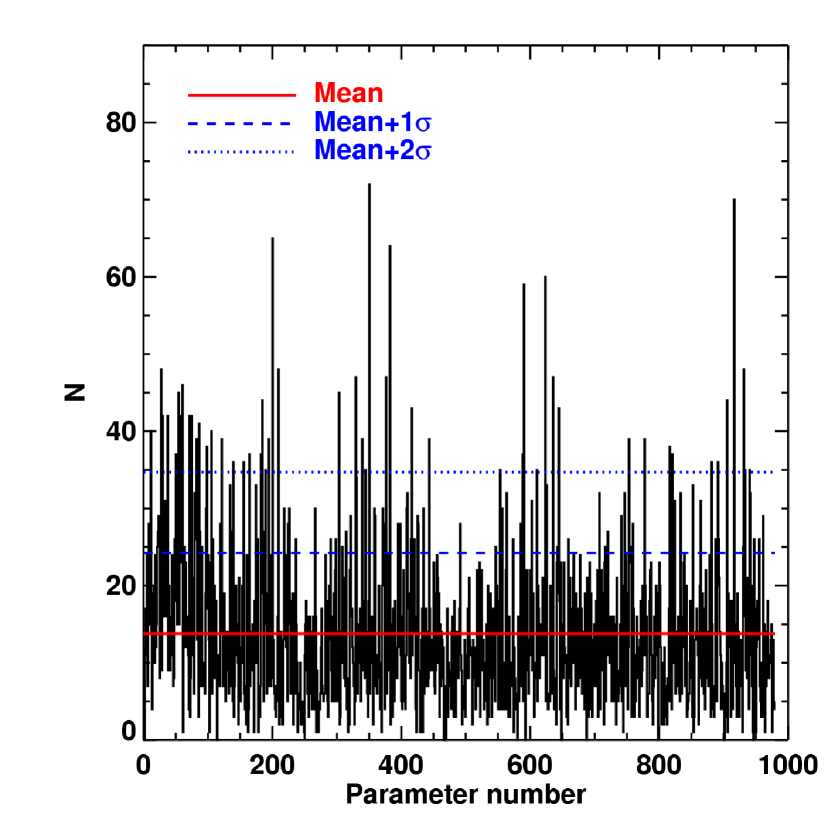
Figure 1.— Example of posterior distribution for the parameters obtained from the GA-SVM. This posterior distribution was derived for the application to photometric redshifts (§4.2). The red solid line shows the average occurence of the parameters; the dashed blue line the occurence at the mean plus one standard deviation, af the dotted blue line the occurence at the mean plus two standard deviations. We use here all parameters which appear more times than the mean plus one standard deviation in the posterior distribution.

3.3.1 SVM parameters optimization

SVM are not ”black boxes”, but come with a well defined formalism, and free parameters to be adjusted. For this application, we use the $\nu$SVM version of the algorithm which allows to control the fractional error and the lower limit on the fraction of support vectors used. We use here $\nu=0.1$. In the case of classification (star/galaxy separation), we are then left with only one free parameter, the inverse of the width of the Gaussian Kernel, $\gamma$ (eq. 1). In the case of regression (photometric redshifts), we have an additional free parameter, the trade off parameter $C$ (see Appendix A).

If not used with caution, machine learning methods can lead to over-fitting : the decision function is biased by the training sample and will not perform well on other samples. In order to avoid over-fitting and optimize the value of $\gamma$ and $C$, we perform 10-fold cross-validation: we divide the sample in 10 subsets; we then perform classification or regression for each subset after training on the 9 other subsets. We perform this cross validation for a grid of $\gamma$ and $C$ values. In the case of SVM, the overfitting can be measured by the fraction of objects used as support vectors, $f_{\rm SV}$. If $f_{\rm SV}\sim 1$, most of the training sample is used as support vectors, will lead to poor generalization. For each iteration, we also get $f_{\rm SV}$, in order to include it on our cost function. For both applications, we minimize a custom cost function that optimizes the quality of the classification or regression, and $f_{\rm SV}$.

4. Results

4.1. Star/Galaxy separation

We use as inputs to the GA feature selection step all magnitudes available for the PS1 dataset: $u_{\rm CFHT}$, $g_{\rm P1}$, $r_{\rm P1}$, $i_{\rm P1}$, $z_{\rm P1}$, and $y_{\rm P1}$; the spread_model values derived from each of these bands; the ellipticity measured on the $\chi^{2}$ image, all colors. We also included a few quantities determined by running the code lephare on these data: photometric redshift, and ratios of the minimum $\chi^{2}$ using galaxy, star, and quasar templates: $\chi^{2}_{\rm galaxy}/\chi^{2}_{\rm star}$, $\chi^{2}_{\rm galaxy}/\chi^{2}_{\rm quasar}$, and $\chi^{2}_{\rm quasar}/\chi^{2}_{\rm star}$. Including the transformations of these parameters yields 96 input parameters to the GA-SVM feature selection procedure.

The parameters selected by the GA with occurence larger than $\mu+\sigma$ times in the posterior distribution are listed in Table 1. We also indicate the parameters whose occurence is larger than $\mu+2\sigma$ times. The 15 selected parameters include spread_model derived in $g_{\rm P1}$, $r_{\rm P1}$ and $i_{\rm P1}$, but are dominated by colors (7 of 15). Using the parameters occuring more than $\mu+2\sigma$ yields similar results, however with significant overfitting.

Table 1Star/Galaxy separation: GA output parameters

Parameter	Transform	Occurence threshold
$u_{\rm CFHT}$	log	$\mu+\sigma$
$r_{\rm P1}$	lin	$\mu+\sigma$
$r_{\rm P1}$	log	$\mu+2\sigma$
spread_model_g	exp	$\mu+\sigma$
spread_model_r	lin	$\mu+2\sigma$
spread_model_r	log	$\mu+2\sigma$
spread_model_i	exp	$\mu+2\sigma$
$u_{\rm CFHT}-g_{\rm P1}$	lin	$\mu+\sigma$
$u_{\rm CFHT}-z_{\rm P1}$	lin	$\mu+\sigma$
$u_{\rm CFHT}-y_{\rm P1}$	lin	$\mu+2\sigma$
$g_{\rm P1}-y_{\rm P1}$	log	$\mu+\sigma$
$r_{\rm P1}-y_{\rm P1}$	exp	$\mu+\sigma$
$i_{\rm P1}-y_{\rm P1}$	lin	$\mu+\sigma$
$z_{\rm P1}-y_{\rm P1}$	exp	$\mu+\sigma$
$z_{\rm phot}$	lin	$\mu+\sigma$

In order to quantify the quality of the star/galaxy separation, we use following definitions for the completeness $c$ and the purity $p$:

$$c_{\rm g} = \frac{n_{\rm g}}{n_{\rm g}+m_{\rm g}}$$ (3)

$$p_{\rm g} = \frac{n_{\rm g}}{n_{\rm g}+m_{\rm s}}$$ (4)

where $n_{\rm x}$ is the number of objects of class $x$ correctly classified, and $m_{\rm x}$ is the number of objects of class $x$ misclassified. The same definition holds for the star completeness and purity.

Based on these definitions, in the case of star/galaxy separation, we use as cost function:

$$\begin{split}J=\left(\frac{c_{\rm g}-1}{0.005}\right)^{2}+\left(\frac{c_{\rm s}-1}{0.005}\right)^{2}+\left(\frac{p_{\rm g}-1}{0.005}\right)^{2}+\left(\frac{p_{\rm s}-1}{0.005}\right)^{2}+\\ \left(\frac{f_{\rm SV}-0.1}{0.01}\right)^{2}.\end{split}$$ (5)

In other words, we choose here to optimize the average completeness and purity for stars and galaxies, and also penalize high $f_{\rm SV}$, which amounts to penalize high fractional errors, and overfitting as well. Other optimization schemes can be adopted. We perform the optimization over the only SVM free parameter here, the inverse of the width of the Gaussian Kernel, $\gamma$. We use a grid search using a $\log$-spaced binning for $0.01<\gamma<10$.

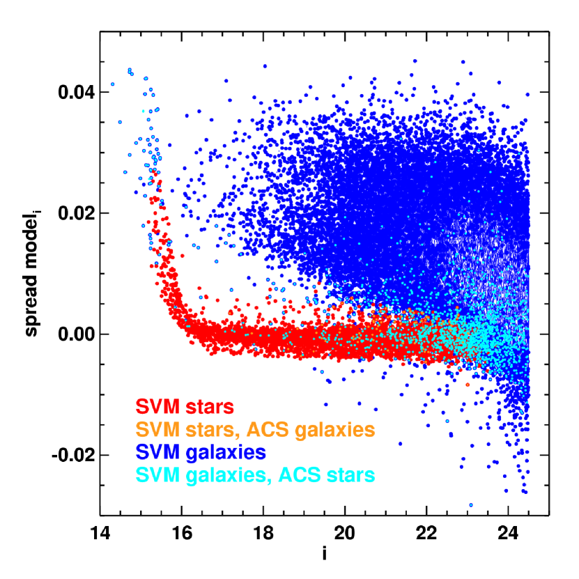
Figure 2.— SExtractor morphological classifier spread_model measured in PS1 $i$ band as a function of $i_{\rm P1}$. We also show the result of our baseline classification (training on all objects): red points show objects classified as stars by the GA-SVM, and blue points objects classified as galaxies. Orange and cyan points show misclassified objects: orange are galaxies according to the catalog of Leauthaud et al. (2007) classified as stars, and cyan stars classified as galaxies.

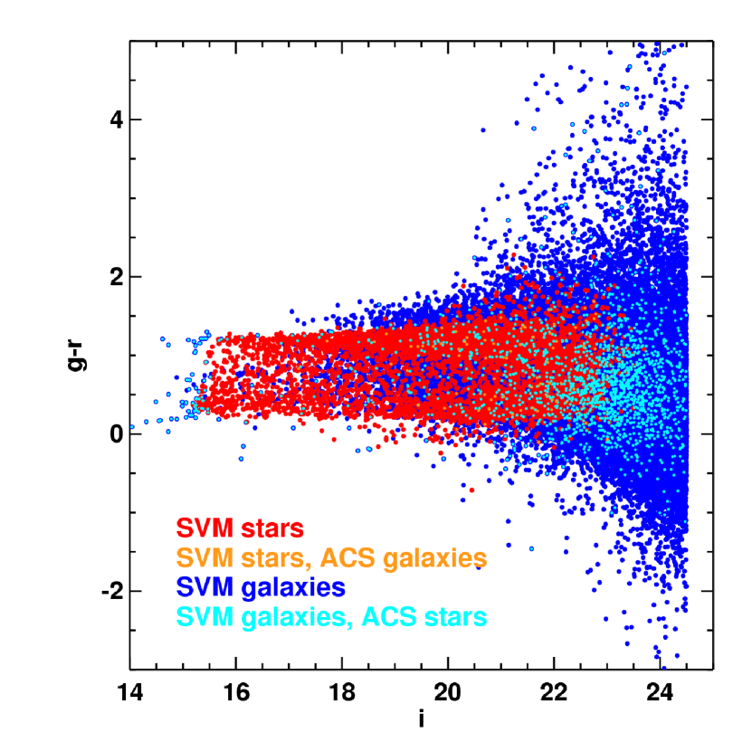
Figure 3.— Color magnitude diagram $g-i_{\rm P1}$ as a function of $i_{\rm P1}$. The color coding is the same as in Fig. 2

We show in Fig. 2 the spread_model derived in the PS1 $i$ band, as a function of $i_{\rm P1}$. Fig. 2 shows that spread_model enables to recover a star sequence down to $i_{\rm P1}\sim 22$. At fainter magnitudes morphology alone is not able to separate accurately stars from galaxies at the PS1 angular resolution. The colors coding shows the result of the GA-SVM classification. We classify objects down to $i_{\rm P1}=24.5$. We choose this limit because the completeness of the PS1 data drops significantly beyond 24.5, and also because the training set we use is valid down to $F814W=25$. Fig. 1 suggests that the GA-SVM is able to recover the classification at bright magnitudes, but also to extend it at the faint end. We list in Table 2 the percentage of objects classified correctly. Our method correctly classifies 97% of the objects down to $i_{\rm P1}=24.5$. We can compare our results to those from the PS1 photometric classification server (Saglia et al., 2012), who used SVM on bright objects using PS1 photometry. They obtained 84.9% of stars correctly classified down to $i_{\rm P1}=21$, and 97% of galaxies down to ${}_{\rm P1}=20$. Our method enables to improve upon those, as we get 88.6% of stars correctly classified, and 99.3% of galaxies correctly classified in the same magnitude range.

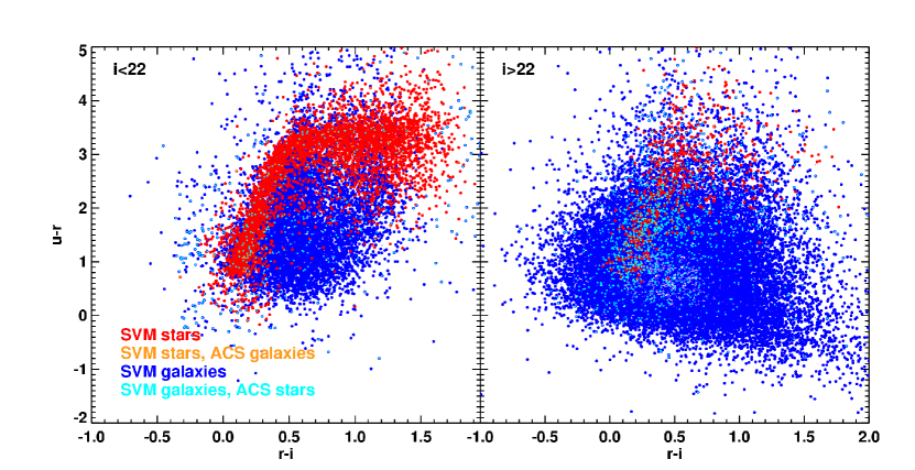
Figure 4.— Color-color diagram $u-r_{\rm P1}$ as a function of $r-i_{\rm P1}$. The left panel shows objects with $i_{\rm P1}<22$ and the right panel objects with $i_{\rm P1}>22$. The color coding is the same as in Fig. 2

We examine in more details in Fig. 3 and 4 the colors of the objects. These figures show that the bulk of stars that are misclassified as galaxies are at the faint end $i\gtrsim 22$, and that these objects are in regions where the colors of stars and galaxies are similar. Galaxies misclassified as stars are brighter $i<22$ but again are in regions where colors of stars and galaxies overlap. There are also a handful of very bright stars misclassified as galaxies, in a domain where the galaxy sampling is very poor. Finally, we classify as galaxies a few stars showing colors at the outskirt of the color distributions. These objects might be either misclassified by the ACS photometry, or the color might be significantly impacted by photometric scatter.

We show in Fig. 5 the completeness (left) and purity (right) of our classifications as a function of $i_{\rm P1}$.

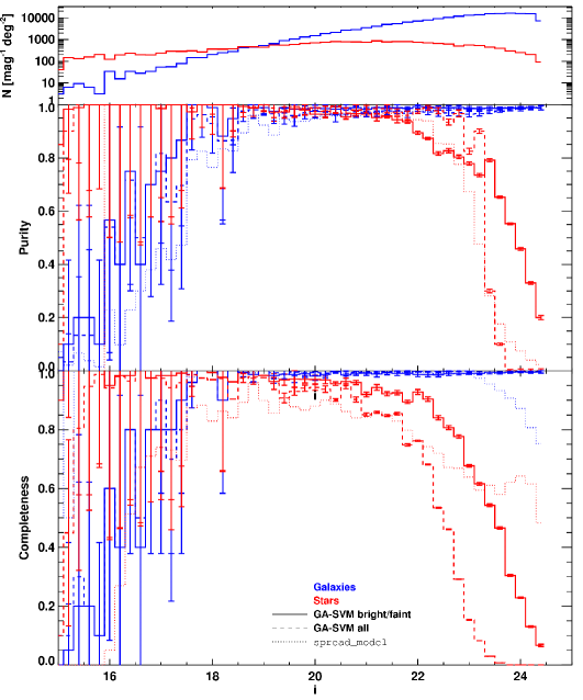
Figure 5.— Quality of the GA-SVM star/galaxy classification. Top: Galaxy and star counts.Middle: completeness as a function of PS1 $i$ magnitude. Bottom: Purity as a function of PS1 $i$ magnitude. On all panels, Red is for stars, and blue for galaxies. On the middle and bottom panels, lines show different classifications: the dashed lines show the result of our classifiction when training with the full sample; solid lines when traing on bright ($i_{\rm P1}>22$) and faint ($i_{\rm P1}<22$) objects separately; dotted lines show the classification from spread_model.

Table 2Star/Galaxy separation: performance

Type	GA-SVM all	GA-SVM bright/faint	spread_model
All types	97.4	98.1	92.7
Galaxies	99.8	99.2	94.5
Stars	74.5	88.5	75.9

Note. — Percentage of correctly classified objects for each method:

We derive the completeness and purity for each cross-validation subset, and show in Fig. 5 the average, and as error bars the standard deviation. Most of the features of our classification seen in Fig. 5 are due to the fact that the training sample is unbalanced at the bright end and the faint end: at the bright end, stars outnumber the galaxies, and the other way around at the faint end. At the bright end ($i_{\rm P1}<16$, which is also within the saturation regime), the completeness is higher for stars than for galaxies, while noisy because of small statistics. Some bright galaxies are misclassified as stars. At the faint end ($i_{\rm P1}>22$), the star completeness decreases, as some stars are classified as galaxies. The impression given by Fig. 5 is striking, as the star completeness decreases to 0 at $i_{\rm P1}\sim 24$. Note however that the stars represent only 3% of the overall population at this flux level (Leauthaud et al., 2007). The purity shows a similar behaviour at the bright end. At the faint end however the stars purity is larger than 0.85 for $i_{\rm P1}\lesssim 23$. For galaxies, both completeness and purity are lower than 0.8 at the bright end ($i_{\rm P1}<18$), however the number of galaxies is small at these magnitudes. At $i_{\rm P1}>18$, completeness and purity are independent of magnitude down to $i_{\rm P1}=24.5$ and larger than 0.95.

We compare this results to the classification obtained with spread_model derived in the $i_{\rm P1}$ band. We determine a single cut in spread_model_i using its distribution for reference stars and galaxies. Our cut is the value of spread_model_i such that $p(\rm{g|\texttt{spread\_model\_i}})=p(\rm{s|\texttt{spread\_model\_i}})$. We show in Fig. 5 the completeness and purity obtained with spread_model_i as dotted lines. For $i_{\rm P1}\lesssim 22$, the results from spread_model_i and our method are similar, as at the PS1 resolution, point sources and extended objects are well discriminated in this magnitude range. At $i_{\rm P1}>22$, our baseline method performs better, in particular for galaxies, which is expected as we add color information. While the galaxies’ purity is similar for both methods, the completeness obtained with spread_model_i drops to 0.75 at $i_{\rm P1}=24.5$, but our methods yields a completeness consistent with 1 down to this magnitude. For stars, the purity obtained with the two methods are similar. On the other hand, the completeness we obtain drops faster than that obtained with spread_model_i. In order to see whether we can improve our baseline method, we optimize the SVM parameters independently in two magnitude range: $i_{\rm P1}<22$ and $i_{\rm P1}>22$. As galaxies at the faint end outnumber stars by several orders of magnitude, we add an extra free parameter for the optimization at $i_{\rm P1}>22$, which attempts at correcting this sampling issue. In practice we use all stars available, but only a fraction of the galaxies available, from 1 to 10 times the number of stars. The results obtained are shown in solid lines on Fig. 5. The results for galaxies are virtually unchanged compared to our baseline method. For stars, we are able to improve at the faint end, where the purity is better than that obtained with spread_model_i for $i_{\rm P1}<23$.

As a final check, we also derive the star/galaxy separation by using SVM only, without selecting the inputs with the GA. The results are only marginally different. We note however that a parameter space with lower dimensions is less prone to overfitting with machine learning methods. On the other hand, even with similar results, a SVM-based star/galaxy separation with smaller number of inputs parameters is more likely to generalize properly.

4.2. Photometric redshifts

We used 978 input parameters as inputs for the GA-SVM optimization procedure: all magnitudes and colors available from the COSMOS dataset and the transformations of these parameters, as described in Sect. 3.3. Hereafter we consider the parameters that appear at least $\mu+1\sigma$ times in the posterior distribution, we are left with 131 parameters. The parameters retained by the GA-SVM are dominated by colors (82%, 108/131), and in particular colors involving intermediate and narrow bands (71%, 93/131). Using the parameters that appear $\mu+2\sigma$ times in the GA posterior distribution yields 45 parameters, with similar proportions of colors and intermediate and narrow bands. This is in line with the conclusions of studies using SED fitting methods which show that including narrow and intermediate bands improves significantly the estimation of photometric redshifts (e.g. Ilbert et al., 2009).

We quantify the errors on photometric redshifts as $err(z_{\rm spec})=(z_{\rm phot}-z_{\rm spec})/(1+z_{\rm spec})$, use as a measure of global accuracy $\sigma$ the normalized median absolute deviation, defined as $\sigma(z)=1.4826*\textrm{median}(|err(z_{\rm spec})-\textrm{median}(err(z_{\rm spec}))|)$.

We define the following cost function for the SVM optimization:

$$J=\left(\frac{\sigma(z)-0.005}{0.0001}\right)^{2}+\left(\frac{f_{\rm SV}-0.1}{0.01}\right)^{2}.$$ (6)

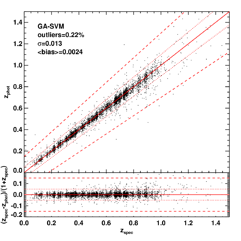
Figure 6.— Top: comparison of spectroscopic redshifts with photometric redshifts obtained with the GA-SVM. The solid line shows identity; the dotted line an error or 0.05 in $1+z$, and the dashed line an error of 0.15 in $1+z$. Bottom: error of photometric redshifts as a function of spectroscopic redshifts. Lines are the same as above.

We perform the optimization over the 2 SVM free parameters available here, $\gamma$, and the trade off parameter $C.$ We use a grid search using a log-spaced binning for $0.01<\gamma<10$ and $0.01<C<500$.

We compare in Fig. 6 spectroscopic and photometric redshifts. We obtain an overall accuracy of 0.013. The percentage of outliers, defined as objects with $|err(z_{\rm spec})|>0.15$, is below 1%. The average error (bias) is equivalent to 0; our results do not show any significant bias as a function of redshift. At high redshifts ($z>1$) the spectroscopic sampling is small, and so the model is less constrained. Using the parameters that appear $\mu+2\sigma$ times in the GA-SVM posterior distribution yields similar results ($\sigma(z)=0.014$), which shows that by using 3 times less parameters, the same accuracy can be achieved.

On a similar sample, Ilbert et al. (2009), using a SED fitting method, obtain an overall accuracy of 0.007. While our results are slightly worse at face value, we note that we use here only 2 free parameters for the photometric redshift optimization, and one model to derive the photometric redshifts (the one from SVM). On the other hand Ilbert et al. (2009) rely on 21 SED templates, 30 zero point offsets (one per band), and an extra parameter describing the amount $E(B-V)$ of internal dust attenuation. We also explicitly avoid overfitting, and doing so guarantees the potential for generalization of these results. Our tests show that we can obtain an overall accuracy of $\sim 0.01$, however this comes at the price of significant overfitting (the support vectors are made up from the whole sample.)

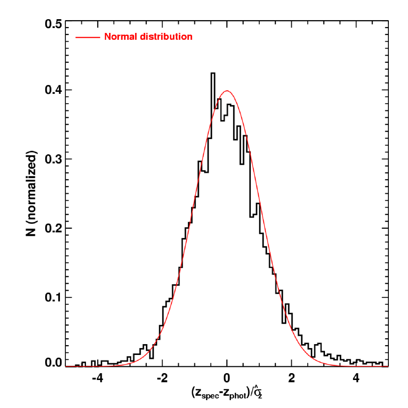
Figure 7.— Empirical estimate of photometric redhift errors. The histogram shows the distribution of the ratio $(z_{\rm spec}-z_{\rm phot})/\hat{\sigma}_{\rm z}$. The curve is a normal distribution.

As above, we also derive the photometric redshifts by using SVM only, without selecting the inputs with the GA. In this case the results are much worse, yielding large errors: $\sigma(z)\sim 0.5$. This shows that the combination of GA and SVM yields better results than SVM alone.

We also test whether we can derive empirical error estimates for each objects using SVM. We use a variant of the $k-$fold cross validation, so-called “inverse”. The usual $k-$fold cross validation consists of dividing the sample into $k$ subsamples (we use $k=10$ here); for each subsample predictions are made using the SVM trained on the union of the other $k-1$ subsamples. To derive error estimates, we use the inverse $k-$fold cross validation such that we train the SVM on one subsample, and predict photometric redshifts for the union of the other $k-1$ subsamples. We have then $k-1$ estimates of $z_{\rm phot}$. We derive an empirical error estimate $\hat{\sigma}_{\rm z}$ which is the standard deviation of these estimates. We show in Fig. 7 the normalized distribution of the ratio $(z_{\rm spec}-z_{\rm phot})/\hat{\sigma}_{\rm z}$. If our empirical estimate were an accurate measurement of the actual error, this distribution should be a Normal one. The comparison with a Normal distribution shows that this is indeed the case, which suggests that our error estimates are accurate.

5. Conclusions

We present a new combination of two machine learning methods that we apply to two common problems in astronomy, star/galaxy separation and photometric redshift estimation. We use Genetic Algorithms to select relevant features, and Support Vector Machines to estimate the quantity of interest using the selected features. We show that the combination of these two methods yields remarkable results, and offers an interesting opportunity for future large surveys which will gather large amount of data. In the case of star/galaxy separation, the improvements over existing methods are a consequence of adding more information, while for photometric redshifts, it is rather the selection of the input information fed to the machine learning methods. This shows that the combination of GA and SVM is very efficient in the case of problems with large dimensions.

We first apply the GA-SVM method to star/galaxy separation in the PS1 Medium Deep Survey. Our baseline method correctly classifies 97% of objects, in particular virtually all galaxies. Our results improve upon the new SExtractor morphological classifier, spread_model, which is expected as we added color information compared to morphology only. We show how these results can be further improved for stars by training separately bright and faint objects, and taking into account the respective number of stars and galaxies to avoid being dominated by one population.

We then apply the GA-SVM method to photometric redshift estimation for the zCOSMOS bright sample. We obtain an accuracy of 0.013, which compares well with results from SED fitting, as we are using only 2 free parameters. We also show that we can derive accurate error estimates for the photometric redshifts.

We present here a proof-of-concept of a new method that can be modified or improved depending on the problem at stake. For instance, one can substitute another machine learning tool to SVM (such as Random Forests for instance) to derive the quantity of interest. Furthermore the criterion used to select the final number of features from the GA posterior distribution can be also be optimized beyond the one we use here. All these tools will enable to use as much information as possible in an efficient way for future large surveys.

Appendix A Support Vector Machines: short description

We provide here a short description of the SVM. More detailed presentations of the formalism can be found elsewhere (e.g. Smola & Schölkopf, 1998; Vapnik, 1995, 1998). For the sake of brevity, we present here only the equations relevant to regression with SVM. Equations for classification are similar, except a few differences that we mention whenever necessary.

The training data usually consists of a number objects with input parameters, $\vec{x}$, of any dimension, and the known values of the quantity of interest, $\vec{y}$. The goal of SVM is to find a function $f$ such as

$$f=\vec{w}.\vec{x}+b$$ (A1)

which yields $\vec{y}$ with a maximal error $\epsilon$, and such as $f$ is as flat as possible. In other words, the amplitude of the slope $\vec{w}$ has to be minimal. One way to achieve this is to minimize the norm $\frac{1}{2}|w|^{2}$ with the condition $|y_{i}-\vec{w}.\vec{x_{i}}-b|\leq\epsilon$. The margin in that case is $\frac{2}{|w|}$. In other words, SVM attempt to regress with the largest possible margin.

In a number of problems, the data can not be separated using a fix, hard margin. It is then useful to allow some points to be misclassified. One uses a ”’soft margin”, which enables to allow some errors in the results. The modified minimization reads:

minimize $$\left.\begin{array}[]{l}\frac{1}{2}|w|^{2}+C\sum_{i}\xi_{i}+\xi_{i}^{*}\\ \end{array}\right.$$ (A3)

$$\textrm{subject to}: \left\{\begin{array}[]{l}y_{i}-w.x_{i}-b\leq\epsilon+\xi_{i}\\ -y_{i}+w.x_{i}+b\leq-\epsilon+\xi_{i}^{*}\\ \xi_{i}\textrm{,}\xi_{i}^{*}\geq 0\end{array}\right.$$ (A7)

where $\xi_{i},\xi_{i}^{*}$ are ”slack variables”, and $C$ is a free parameter which controls the soft margin. The larger $C$, the harder the margin: larger error are penalized.

Using Lagrange multiplier analysis, it can be shown that the slope $w$ can be written as:

$$w=\sum_{i=1}^{n}(\alpha_{i}-\alpha_{i}^{*})x_{i}$$ (A8)

where $\alpha_{i},\alpha_{i}^{*}$ are the Lagrange multipliers, which satisfy $\sum_{i=1}^{n}\alpha_{i}-\alpha_{i}^{*}=0$, and $\alpha_{i},\alpha_{i}^{*}\in[0,C]$.

Eq. A8 shows that the solution of the minimization problem is a linear combination of a number of input data points. In other words, the solution is based on a number of support vectors, the number of training samples where $\alpha_{i}-\alpha_{i}^{*}\neq 0$.

The above equations use the actual values of the data, assuming that the separation can be performed linearly. For most high dimension problems, this assumption is not valid any more. The fact that only a scalar product between the support vectors and the input data is required enables to use the so-called ”kernel trick”. The idea behind the trick is that one can use functions which satisfy a number of conditions to map the input space to another where the separation can be performed linearly. Eq. A8 then becomes:

$$w=\sum_{i=1}^{n}(\alpha_{i}-\alpha_{i}^{*})\Phi(x_{i})$$ (A9)

where the kernel $k(x,x^{\prime})=\langle\Phi(x)\Phi(x^{\prime})\rangle$.

Finally, a slightly modified version of the algorithm ($\nu$SVR) allows to determine $\epsilon$ and control the number of support vector. A parameter $\nu\in[0,1]$ is introduced such that Eq. A3 becomes

$$\textrm{minimize}\quad\frac{1}{2}|w|^{2}+C(\nu\epsilon+\sum_{i}\xi_{i}+\xi_{i}^{*}).$$ (A10)

It can be shown that $\nu$ is the upper limit on the fraction of errors, and the lower limit of the fraction of support vectors.

In the regression case described here, the free parameters for $\nu$SVR are the trade off parameter $C$ and all the kernel parameters (assuming that one fixes $\nu$, which allows control of the error and the fraction of support vectors). In the classification case ($\nu$SVC), the free parameters are only those from the kernel which is used, as $\nu$ replaces the trade off parameter $C$, and again, one would usually fix $\nu$.

References

- Alba et al. (2007) Albda, E., Garcia-Nieto, J., Jourdan, L., Talbi, E.-G. 2007, Congress on Evolutionary Computation
- Arnouts et al. (1999) Arnouts, S., Cristiani, S., Moscardini, L., et al. 1999, MNRAS, 310, 540
- Benítez (2000) Benítez, N. 2000, ApJ, 536, 571
- Bertin & Arnouts (1996) Bertin, E., & Arnouts, S. 1996, A&AS, 117, 393
- Bertin et al. (2002) Bertin, E., Mellier, Y., Radovich, M., et al. 2002, Astronomical Data Analysis Software and Systems XI, 281, 228
- Bertin (2011) Bertin, E. 2011, Astronomical Data Analysis Software and Systems XX, 442, 435
- Boser et al. (1992) Boser, B. E., Guyon, I. M., Vapnik, V. N. 1992, Proceedings of the 5th Annual ACM Workshop on Computational Learning Theory, 144
- Brammer et al. (2008) Brammer, G. B., van Dokkum, P. G., & Coppi, P. 2008, ApJ, 686, 1503
- Budavári (2009) Budavári, T. 2009, ApJ, 695, 747
- Cantó et al. (2009) Cantó, J., Curiel, S., & Martínez-Gómez, E. 2009, A&A, 501, 1259
- Capak et al. (2007) Capak, P., Aussel, H., Ajiki, M., et al. 2007, ApJS, 172, 99
- Carliles et al. (2010) Carliles, S., Budavári, T., Heinis, S., Priebe, C., & Szalay, A. S. 2010, ApJ, 712, 511
- Cavuoti et al. (2014) Cavuoti, S., Garofalo, M., Brescia, M., et al. 2014, New Astronomy, 26, 12
- Cawley & Talbot (2010) Cawley, G.,& Talbot, N. 2010, Journal of Machine Learning Research, 11, 2079
- Collister et al. (2007) Collister, A., Lahav, O., Blake, C., et al. 2007, MNRAS, 375, 68
- Connolly et al. (1995) Connolly, A. J., Csabai, I., Szalay, A. S., et al. 1995, AJ, 110, 2655
- Conroy et al. (2010) Conroy, C., White, M., & Gunn, J. E. 2010, ApJ, 708, 58
- Cortes & Vapnik (1995) Cortes, C., Vapnik, V. N. 1995, Machine Learning, 20, 273
- Duda et al. (2001) Duda, R. O., Hart, P. E., Stork, D. G. 2001, Pattern Classification, Wiley
- Fadely et al. (2012) Fadely, R., Hogg, D. W., & Willman, B. 2012, ApJ, 760, 15
- Fatemi & Gharaghani (2007) Fatemi, M. H., Gharaghani, S. 2007, Bioorganic & Medicinal Chemistry, 15, 24, 7746
- Hogan et al. (2015) Hogan, R., Fairbairn, M., & Seeburn, N. 2015, MNRAS, 449, 2040
- Huerta et al. (2006) Huerta, E. B., Duval, B., Hao, J.-K. 2006, Applications of Evolutionary Computing, 3907, 34
- Huertas-Company et al. (2011) Huertas-Company, M., Aguerri, J. A. L., Bernardi, M., Mei, S., & Sánchez Almeida, J. 2011, A&A, 525, A157
- Ilbert et al. (2009) Ilbert, O., Capak, P., Salvato, M., et al. 2009, ApJ, 690, 1236
- Ivezic et al. (2008) Ivezic, Z., Tyson, J. A., Abel, B., et al. 2008, arXiv:0805.2366
- Kaiser et al. (2010) Kaiser, N., Burgett, W., Chambers, K., et al. 2010, Proc. SPIE, 7733, 77330E
- Kron (1980) Kron, R. G. 1980, ApJS, 43, 305
- Kovács & Szapudi (2015) Kovács, A., & Szapudi, I. 2015, MNRAS, 448, 1305
- Krone-Martins et al. (2014) Krone-Martins, A., Ishida, E. E. O., & de Souza, R. S. 2014, MNRAS, 443, L34
- Laureijs et al. (2011) Laureijs, R., Amiaux, J., Arduini, S., et al. 2011, arXiv:1110.3193
- Leauthaud et al. (2007) Leauthaud, A., Massey, R., Kneib, J.-P., et al. 2007, ApJS, 172, 219
- Lilly et al. (2007) Lilly, S. J., Le Fèvre, O., Renzini, A., et al. 2007, ApJS, 172, 70
- Liu et al. (2012) Liu, C., Bailer-Jones, C. A. L., Sordo, R., et al. 2012, MNRAS, 426, 2463
- Magnier (2006) Magnier, E. 2006, The Advanced Maui Optical and Space Surveillance Technologies Conference, 50
- Min et al. (2006) Min, S.-H., Lee, J., Han, I. 2006, Expert Systems with Applications, 31, 3, 652
- Nesseris (2011) Nesseris, S. 2011, Journal of Physics Conference Series, 283, 012025
- Pedregosa et al. (2011) Pedregosa, F., Varoquaux, G., Gramfort, A., et al. 2011, Journal of Machine Learning Research, 12, 2825
- Rahman et al. (2015) Rahman, M., Ménard, B., Scranton, R., Schmidt, S. J., & Morrison, C. B. 2015, MNRAS, 447, 3500
- Rest et al. (2014) Rest, A., Scolnic, D., Foley, R. J., et al. 2014, ApJ, 795, 44
- Robin et al. (2007) Robin, A. C., Rich, R. M., Aussel, H., et al. 2007, ApJS, 172, 545
- Sanders et al. (2007) Sanders, D. B., Salvato, M., Aussel, H., et al. 2007, ApJS, 172, 86
- Saglia et al. (2012) Saglia, R. P., Tonry, J. L., Bender, R., et al. 2012, ApJ, 746, 128
- Scoville et al. (2007) Scoville, N., Aussel, H., Brusa, M., et al. 2007, ApJS, 172, 1
- Small et al. (2013) Small, E. E., Bersier, D., & Salaris, M. 2013, MNRAS, 428, 763
- Smola & Schölkopf (1998) Smola, A. J., Schölkopf, NeuroCOLT Technical Report NC-TR-98-030
- Soumagnac et al. (2013) Soumagnac, M. T., Abdalla, F. B., Lahav, O., et al. 2013, arXiv:1306.5236
- Spergel et al. (2015) Spergel, D., Gehrels, N., Baltay, C., et al. 2015, arXiv:1503.03757
- Steeb (2014) Steeb, W. H. 2014, The Nonlinear Workbook, World Scientific
- Stoughton et al. (2002) Stoughton, C., Lupton, R. H., Bernardi, M., et al. 2002, AJ, 123, 485
- Szalay et al. (1999) Szalay, A. S., Connolly, A. J., & Szokoly, G. P. 1999, AJ, 117, 68
- Taniguchi et al. (2007) Taniguchi, Y., Scoville, N., Murayama, T., et al. 2007, ApJS, 172, 9
- Tonry et al. (2012) Tonry, J. L., Stubbs, C. W., Lykke, K. R., et al. 2012, ApJ, 750, 99
- Vapnik (1995) Vapnik V. N. 1995, The Nature of Statistical Learning Theory, Springer-Verlag
- Vapnik (1998) Vapnik V. N. 1998, Statistical Learning Theory, Wiley
- Vasconcellos et al. (2011) Vasconcellos, E. C., de Carvalho, R. R., Gal, R. R., et al. 2011, AJ, 141, 189
- Wadadekar (2005) Wadadekar, Y. 2005, PASP, 117, 79
- Woźniak et al. (2004) Woźniak, P. R., Williams, S. J., Vestrand, W. T., & Gupta, V. 2004, AJ, 128, 2965
- Zhang & Zhao (2004) Zhang, Y., & Zhao, Y. 2004, A&A, 422, 1113