Biological hierarchies emerged from natural characteristics of a number theory

Abstract

We would like to show how biological grouping, especially in the case of species formation, is emerged through a nature of interactive populations with a number theory. First, we are able to define a species as a $p$-Sylow subgroup of a particular community in a single niche, confirmed by topological analysis. We named this model the patch with zeta dominance (PzDom) model. Next, the topological nature of the system is carefully examined. We confirm the induction of hierarchy and time through a one-dimensional probability space with certain topologies. For further clarification of induced fractals including the relation to renormalization, a theoretical development is proposed based on a newly identified fact, namely that scaling parameters for magnetization analogs exactly correspond to imaginary parts of the Riemann zeta function’s nontrivial zeros. In our PzDom model, calculations only require knowledge of the density of individuals over time.

1 Introduction

Living organisms mainly have three characters in contrast to non-organic materials: reproduction, metabolism and compartmentalization. These characters are all important for maintaining their own identities, aiming to be reproductive with high fitness rates. However, the definitions lack the social aspects of the organisms. The society of life is not a mere aggregation of mutually independent individuals. It does include social interactions for even higher fitness rates. Grouping of the individuals based on the relational aspects of the living organisms is thus important and may act as another characteristic of the organisms. The problem here is how ‘grouping’ can be appropriately defined in the context of reproduction.

Group selection is a proposed mechanism of evolution in life, in which natural selection acts at the level of groups, instead of the level of individuals or genes. However, it would not occur in an ultimate level with infinite time and space, because the non-rewarded cost to support non-relative individuals would eliminate the individuals with such a character during evolution. Naive group selections are thus difficult to occur, and biologists propose other types of selection mechanisms: kin selection/inclusive fitness theory and multilevel selection. Kin selection is a selection mechanism that acts on relative individuals. The cooperation of these individuals are thus possible to increase their fitness regarding the relatedness of them. It is evidently true in many taxa, e.g. in eusocial insects. For marking relatives, green beard gene is discussed to give a signal that they are the cooperators. On the other hand, multilevel selections act on multilevels, not only on an individual level. The hierarchies of life system can be interpreted as a result of selections acting on different levels; however, this theory is rather hypothetical except the case in human beings [Sober and Wilson, 1998].

Biological systems compose of various levels of hierarchies; i.e. molecule, cell, tissue, organ, organ system, (individual) organism, population, community, ecosystem and biosphere. Theoretically, this character might be arised from natures of thermodynamical open systems and set theoretical natures of dissipative structures. However, detailed theories of this phenomena are still obscure. In order to explain the origins of these hierarchies, we focus on one of the mysterious concepts among the hierarchies - ‘species’. Currently, there are various ways to define a species, and none of these is uniformly applicable to phenomena considered in the context of biology. For example, biological species concept is stated as “groups of actually or potentially interbreeding natural populations, which are reproductively isolated from other such groups”. Although this species concept is experimentally quantifiable and the most well-defined concept compared to others, it cannot be applied to asexual living organisms that do not mate each other. Ring species are another example that cannot be applicable for this species concept. For others, morphological species concept, “a group of organisms in which individuals conform to certain fixed properties”, can be applied only when the characteristics of interests have discrete natures so as to distinguish a pair of species well. Cryptic species demonstrate an example that cannot be applicable for this species concept. Evolutionary species concept, “an entity composed of organisms which maintains its identity from other such entities through time and over space, and which has its own independent evolutionary fate and historical tendencies”, has arbitrary nature because it is not clear what extent of divergence and distant-related phylogeny can necessarily and sufficiently cause the difference of species level. It is quite often confused with population concept. Although it is important to have a common definition of species in order to compare the dynamics of communities (sets of populations from different species) of various biological taxa, there is still no perfectly proper definition of species for the problem.

What we want here is by a mathematical convergence mechanism utilizing ‘exponential’ and ‘log’-like functions, a demonstration of clear-cut definitions of species, and in further sense interactions of the species. They should be qualitatively defined based on quantitative calculations. Previously, we demonstrate population can be interpretable in the context of Hubbell’s unified neutral theory [Hubbell, 1997] [Hubbell, 2001](or, MaxEnt theories; e.g. [Phillips et al., 2006]), while temporal species can be interpretable as more adaptive concept [Adachi, 2015]. This might be the clue to solve the problem of species definition, because different levels of biological hierarchies - namely, population and species - have distinct characteristics that can be evaluated by the number of individuals classified in the mean of population criterion or species criterion. We would like to develop the logic further, by utilizing an adaptation concept combined with a number theory in mathematics. First, we would like to develop a metric that can distinguish the border of population dynamics (associated with chaotic behavior) and species dynamics (associated with directional adaptation/disadaptation). In the mean time, we would like to utilize a theory that resembles quantum mechanics, because in this line we can treat concepts of quantization (discrete natures of species) and wave functions (functions that describe species-species interaction) as different aspects of the same entity. Regarding this step, one can understand how ‘interaction’ and ‘independency’ can be deciphered in the context of mathematics. Of course, there are some differences among microscopic quantum mechanics in physics and the theory developed here. We would carefully treat the differences later.

2 Results

2.1 Universal equation for population/species dynamics based on the Price equation and logarithms

First of all, we will intorduce exponential- and log-like functions to achieve convergence of the indicators to certain discrete values. The neutral logarithmic distribution of ranked biological populations, for example, a Dictyostelia metacommunity [Adachi, 2015], can be expressed as follows:

$$N_{k}=a-b\ln k,$$ (1)

where $N$ is the population density or the averaged population density of species over patches, and $k$ is the index (rank) of the population. The parameters $a\approx N_{1}$ and the rate of decrease $b$ are derived from the data by sorting the populations by number ranks. We also applied this approximation to an adaptive species to evaluate the extent of their differences from neutral populations [Adachi, 2015]. We note that this approximation is only applicable to communities that can be regarded as existing in the same niche, and not to co-evolving communities in nonoverlapping niches.

Based on the theory of diffusion equations with Markov processes, as used in population genetics [Kimura, 1964], we assume that the relative abundance of the populations/species is related to the $N$th power of $D$ ($=\bar{w}$ in [Kimura, 1964]) multiplied by the relative patch quality $P$ ($=C$ in [Kimura, 1964]) (that is, $PD^{N_{k}}=C\bar{w}^{N_{k}}=\phi=N_{k}/\Sigma N$; see also [Kimura, 1964]). In this context, $D^{N_{k}}$ represents the relative fitness of an individual; this varies over time and depends on the particular genetic/environmental background and the interactions between individuals. $P$ is a relative environmental variable and depends on the background of the occupying species; it may differ within a given environment if there is a different dominant species.

To better understand the principles deduced from Kimura’s theory, we introduce the Price equation [Price, 1970]:

$$w_{k}\Delta z=\mathrm{Cov}(w_{k},z_{k})+E(w_{k}\Delta z_{k}).$$ (2)

Remember $N_{1}=kN_{k}$ when the distribution is completely harmonic (neutral). Note that $z=\ln(k\cdot N_{k})/\ln k=1+\ln N_{k}/\ln k$, where $k\neq 1$ and $z=+\infty$ when $k=1$; we use this instead of gene frequency in Price’s original paper. Furthermore, $w_{k}$ appears as a selection coefficient, not the fitness itself. The relative distance between the logarithms of norms $N$ and the rank $k$ will be discussed later when we consider the Selberg zeta analysis [Juhl, 2001]; here, $\ln k$ is the relative entropy from a uniform distribution as $a$ (in other words, it s a Kullback-Leibler divergence $D_{1}(P||Q)=\sum_{i=1}^{n}p_{i}\ln\frac{p_{i}}{q_{i}}$ of $n=1,p_{i}=1,q_{i}=1/k$, the interaction probability from the first ranked population/species; thus we are able to calculate the deviation from a logarithmic distribution, and both logarithms, $\ln N_{k}$ and $\ln k$, are topological entropies). Next, we assume that for a particular patch, the expectation of the individual populations/species is the averaged (expected) maximum fitness; this is $D$ to the power $E(\Sigma N)$th, when $E(\Sigma N)$ is the average $N$ among all populations or the sum of the average $N$ over all patches among all species ($|D_{k}|^{E(\Sigma N)}$). This is a virtual assumption for a worldline (the path of an object in a particular space) because a population seems to be in equilibrium when it follows a logarithmic distribution [Hubbell, 1997] [Hubbell, 2001] [Adachi, 2015] and species dominate [Adachi, 2015]. We will prove below that the scale-invariant parameter small $s$ indicates adaptations in species in neutral populations. Under the assumptions in this paragraph, $E[w]$ is $|D_{k}|^{E(\Sigma N)}$ and $E[z]$ is approximately $\ln N_{1}/\ln k$. If we set $w=|D_{k}|^{E(\Sigma N)}-\Delta z$, $N_{k}=D^{N_{k}}$ and $k\neq 1$, $\Delta z\approx\Delta N_{k}\ln D_{k}/\ln k$ with $D_{k}\sim 1$. When $k=1$, $\Delta z=\infty$ but $\Delta z$ is removed from the calculation by an identical $\Delta z$ anyway, upon introduction of the equation below. Dividing the Price equation by $\Delta z$, we obtain

$$w_{k}=\frac{\ln\frac{N_{1}}{N_{k}}}{\ln k}-1+|D_{k}|^{E(\Sigma N)}(k\neq 1).$$ (3)

Recall $N_{1}=kN_{k}$ when the distribution is harmonic (normal). In this case, $\ln\frac{N_{1}}{N_{k}}=\ln k$ and $\frac{\ln\frac{N_{1}}{N_{k}}}{\ln k}$ becomes $1$. The value of this calculation represents the deviation from the harmonic (neutral) distribution. We will consider the case when $k=1$ in a later subsection; see Eqns. (12) and (13). For simplicity, we denote $1+\mathrm{Cov}/\Delta z:\frac{\ln\frac{N_{1}}{N_{k}}}{\ln k}$ as $\Re(s)$ and $E(w_{k}):|D_{k}|^{E(\Sigma N)}$ as $\Im(s)$. Now think of a Dirichlet series $\sum_{j=1}^{\infty}b_{Dj}l_{Dj}^{s}$. An upper limit of box dimension of this system $A$ (a subset of $\mathbb{R}^{2}$)is:

$$\overline{\dim}_{B}A=\underset{n\to\infty}{\lim\sup}\frac{1}{\ln l_{Dn}^{-1}}\ln(\sum_{j=1}^{n}b_{Dj})$$ (4)

[Cahen, 1894]. If we regard $\underset{n\to\infty}{\lim}\sum_{j=1}^{n}b_{Dj}=\frac{N_{1}}{N_{k}}$ and $\underset{n\to\infty}{\lim}l_{Dn}=\frac{1}{k}$, such a Dirichlet series fulfilling this condition is characteristic of the model we are considering; dimensions large enough can achieve such approximations close to $\lim$. When $s=1$, the Dirichlet series will be a set of: $\frac{N_{1}}{kN_{k}}$, the deviation from logarithmic distribution of $N$, setting a datum point as 1.The discreteness would be checked in later sections, especially in Figure 1 and Table 1.

2.2 Introducing $\Re(s)$ allows us to distinguish types of neutrality

Zipf’s law is used to statistically analyze probability distributions that follow a discrete power law. For example, if the distribution of $N$ can be approximated by a logarithmic relation with parameter $k$, then Eqn. (1) holds. Zipf’s law is related to the Riemann zeta function $\zeta(s)=\sum_{n=1}^{\infty}\frac{1}{n^{s}}$ as follows:

$$|P_{k}||D|^{N_{k}}=f_{s}(k)=\frac{1}{k^{\Re(s)}|\zeta(s)|}=\frac{N_{k}}{E(\Sigma N)},$$ (5)

and this will normalize the $k$th abundance by $E(\Sigma N)$. We set absolute values of $|\zeta|$ and $|P_{k}|$ for approximating both the $\Re(s)>1$ ($\zeta>0$, $N_{k}<N_{1}/k$) and $\Re(s)<1$ ($\zeta<0$, $N_{k}>N_{1}/k$) cases. Note that this model is a view from the first-ranked population, and either cooperation or competition is described by the dynamics/dominancy of the populaton. To examine the difference between population and species dynamics, linearization of the above model leads to

$$\frac{\Delta N_{k}}{E(\Sigma N)}=-\frac{\Delta\zeta}{k^{\Re(s)}|\zeta|^{2}}.$$ (6)

Therefore, $\Delta N_{k}>0$ implies $\Delta\zeta<0$, $\Delta N_{k}<0$ implies $\Delta\zeta>0$, and $\Delta N_{k}=0$ implies $\Delta\zeta=0$. Each of the local extrema of $\zeta$ thus represents a pole for the population/species, and a large (resp. small) value of $|\zeta|$ represents a small (resp. large) fluctuation. Only those points of $\zeta$ that are close to zero represent growth bursts or collapses of the population/species. According to the Riemann hypothesis, at these points, the following equation will hold $[\Re(s)=1/2]$ and $[\Re(s)=-2l_{s},\Im(s)=0]$ (negative values for $s$ will be characterized later), where $l_{s}$ is a natural number independent of the population/species rank.

Taking the logarithm of Eqn. (5), we obtain

$$N_{k}=\frac{1}{\ln D_{k}}\ln\frac{1}{P_{k}\zeta(s)}-\frac{s}{\ln D_{k}}\ln k,$$ (7)

$$-\ln D_{k}\cdot N_{k}=\ln P_{k}\zeta(s)+s\ln k.$$ (8)

Therefore,

$$a=\frac{-\ln P_{k}\zeta(s)}{\ln D_{k}},$$ (9)

$$b=\frac{s}{\ln D_{k}},$$ (10)

$$\Re(s)=\frac{\ln\frac{N_{1}}{N_{k}}}{\ln k}(k\neq 1),$$ (11)

$$\zeta(s)=\frac{E(\Sigma N)}{N_{1}}\geq 1\ (k=1\mathrm{\ in\ species}),$$ (12)

$$\Re(s)=1\ (k=1\mathrm{\ in\ population/observer}),$$ (13)

$$D_{k}=e^{\frac{s}{b}},$$ (14)

$$P_{k}=\frac{1}{D_{k}^{a}\zeta(s)}.$$ (15)

$\Re(s)$ is obviously scale invariant if $k$ is a fixed number in a particular system. Note that $s$ and $\zeta(s)$ can thus be approximated using data from the distribution of $N$. When $k=1$ for a given population, $s$ can be defined as $1$ because the distribution is almost harmonic. When $k=1$ for a given species, $s$ can be better calculated by an inverse function of $\zeta$, because in this situation the distribution is no longer harmonic. For convergence, it is necessary that $N\sim 0$, $s\sim 1$, $\zeta\sim\pm\infty$, and $P\sim 0$. We will also assume that $s=+\infty$ and $\zeta=1$ when a single population/species is observed. In [Adachi, 2015], we analyzed $s$ values using both the relative abundances of the population and the species; we determined that they give significantly different results (see Figure 1 and Table 1). The population values are restricted to between $0$ and $2$, while those of the species are often greater than $2$. This proves that populations behave neutrally below $\dim_{B}A=2$, while species are more likely to dominate above $\dim_{B}A=2$; this will be discussed in more detail below. When $s$ is larger than $2$, the dynamics correspond to that of species, as will be discussed below. In Table 1, 6/54 $s$ values greater than 2 are highlighted in red; this indicates that these were not observed in a population of 162 samples ($p\sim 4\times 10^{-45}$ for $\chi^{2}$-test). In the following, the parameter $s$ is the small $s$ of this model. Note that when $k\neq 1$, the calculation of $\Re(s)$ is the same for both a population and a species, and the border $\Re(s)=2$ clarifies the distinction of a neutral population ($0<\Re(s)<2$) versus a dominant species ($\Re(s)>2$) as expected in the fractal theory described earlier.

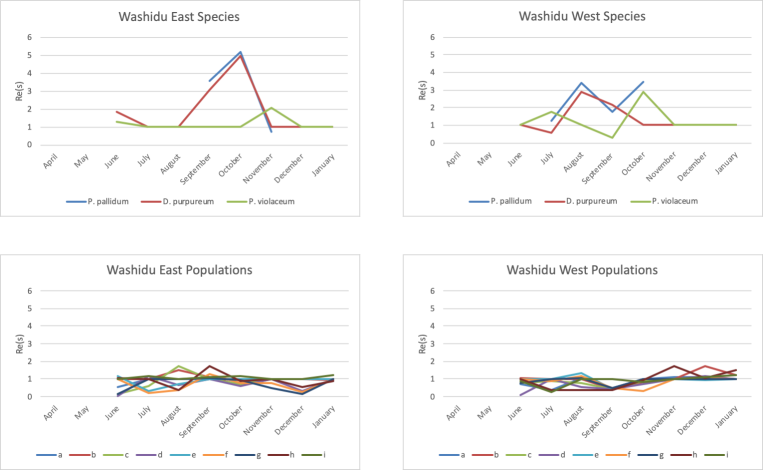
Figure 1: Dynamics of $\Re(s)$ over time for species and populations in two quadrats. P. pallidum: Polysphondylium pallidum; D. purpureum: Dictyostelium purpureum; P. violaceum: Polysphondylium violaceum. The top two panels present data for three different species, and the lower two panels present data for nine different point quadrats.

Table 1: $\Re(s)$ and $N$ values.

$\Re(s)$	P. pallidum (WE)	D. purpureum (WE)	P. violaceum (WE)	P. pallidum (WW)	D. purpureum (WW)	P. violaceum (WW)
April	1	-	1	1	-	1
June	0.7693	1.8305	1.258	-	1	1
July	-	1	1	1.2619	0.5752	1.7742
August	-	1	1	3.4223	2.8795	1
September	3.5762	3.0777	1	1.7897	2.1411	0.3186
October	5.1648	4.9423	1	3.4417	1	2.9047
November	0.7481	1	2.056	-	1	1
December	-	1	1	-	1	1
January	-	1	1	-	1	1
$N$	P. pallidum (WE)	D. purpureum (WE)	P. violaceum (WE)	P. pallidum (WW)	D. purpureum (WW)	P. violaceum (WW)
April	0	76	0	0	83	0
June	123	209	52	147	0	0
July	1282	0	0	80	215	320
August	1561	0	0	1330	181	0
September	901	107	0	809	77	649
October	1069	35	0	799	0	107
November	60	0	101	336	0	0
December	190	0	0	711	0	0
January	29	0	0	99	0	0

$\Re(s)$ WE	a	b	c	d	e	f	g	h	i
April	1.0336	1	1.9442	1	1	1	1.0821	1	1
June	0.5328	1	0.1545	0.0332	1.1928	1	0.1374	1.076	1.0071
July	1	1	0.6131	1.1497	0.3117	0.2016	1	1	1.148
August	1	1.4925	1.7167	0.6348	0.7075	0.3523	1	0.3502	1
September	1	1.1361	1	1	1	1.3035	1.0325	1.7248	1.085
October	1	0.6746	0.6937	0.6092	1	0.7836	0.9259	0.886	1.1746
November	1	1	1	1	1	0.7481	0.472	1	1
December	1	1	1	0.3429	1	0.2455	0.1712	0.5647	1
January	1	0.9516	1	1	1	1	1	0.8666	1.215
$\Re(s)$ WW	a	b	c	d	e	f	g	h	i
April	1	1	0.7125	0.8782	1	1	1	1	1.473
June	0.708	1.0735	0.7614	0.1056	1	1	0.7883	1	0.8612
July	0.3888	1	0.8635	1	1	0.8614	1	0.3629	0.263
August	1.0524	1	0.756	0.5644	1.3367	1.1911	1.0473	0.3985	1
September	0.4918	0.4236	0.4243	0.4427	0.4535	0.4969	0.5051	0.3985	1
October	1	0.8073	0.8982	0.6913	1	0.3219	1	0.9284	0.8523
November	1.1334	1	1	1	1	1	1	1.7225	1
December	1.1214	1.7164	1	1.1833	0.9208	1.0718	1	1.0594	1.1375
January	1	1.2501	1	1	1	1	1	1.5151	1.2228
$N$ WE	a	b	c	d	e	f	g	h	i
April	680	0	94	0	0	1392	424	0	0
June	1120	0	2131	2580	221	2640	2270	384	372
July	0	0	1573	469	2613	3200	3680	0	580
August	0	331	170	1728	1800	3760	0	3267	4800
September	0	1240	0	4320	0	418	820	1307	960
October	0	1413	1680	2360	3600	1020	594	736	313
November	0	0	0	907	0	540	540	0	0
December	0	0	0	580	0	787	773	376	933
January	0	457	0	0	1300	0	0	391	560
$N$ WW	a	b	c	d	e	f	g	h	i
April	840	0	384	457	0	0	0	0	109
June	1088	421	869	3160	0	0	1140	3400	1320
July	1680	0	613	0	0	720	2880	1933	2400
August	704	0	1627	2496	288	457	860	3520	4640
September	1760	1760	1627	1386	1440	2016	1147	2640	3480
October	3520	960	613	1350	0	2816	0	667	1380
November	760	0	0	0	0	0	2640	800	0
December	590	124	0	440	1600	784	4400	1013	2000
January	1307	331	0	0	0	0	0	160	560

WE: the Washidu East quadrat; WW: the Washidu West quadrat (please see [Adachi, 2015]. Scientific names of Dictyostelia species: P. pallidum: Polysphondylium pallidum; D. purpureum: Dictyostelium purpureum; and P. violaceum: Polysphondylium violaceum. For calculation of $\Re(s)$, see the main text. $N$ is number of cells per 1 g of soil. Species names for Dictyostelia represent the corresponding values. a - i indicate the indices of the point quadrats. Red indicates $\Re(s)$ values of species that were approximately integral numbers greater than or equal to 2.

If $D_{k}\sim 1$, there are two possibilities: (i) $P_{k}\approx 1/\zeta(s)\approx\Sigma\mu(n)/n^{s}$ (where $\mu$ is the Möbius function) must be true for $a$ to converge, and for $b$ to converge, we need $s\sim 0$; (ii) For $N$ to converge, we need $s\sim 1$ when $P_{k}<<1$. In this case, we have $kP_{k}\approx 1/\zeta(s)$. When (i) holds, we have true neutrality among the patches. Both (i) and (ii) can be simply explained by a Markov process for a zero-sum population, as described in Hubbell (2001). In both cases, $f_{s}(k)\sim P_{k}$, and the populations are apparently neutral for $D$. When there is true neutrality in both the populations and the environment, $P_{k}\approx 1/\zeta(s)\approx\Sigma\mu(n)/n^{s}$, we say that there is Möbius neutrality. When there is apparent neutrality of $D$ with $s\sim 1$, we say that there is harmonic neutrality. The value of $s$ can thus represent the characteristic status of a system. We now consider situations in harmonic neutrality. $\Re(s)>2$ is an indicator of adaptation beyond the effects of fluctuation from individuals with harmonic neutrality. Also note that $\mu(n)$ represents the bosonic $1$ with an even number of prime multiplications, the fermionic $-1$ with an odd number of multiplications, or $0$ as the observant, which can be divided by a square of prime. This occurs when two quantized particles interact. Note that in about 1400 CE, Madhava of Sangamagrama proved that

$$\sum_{n:odd}(-1)^{(n-1)/2}/n=\pi/4.$$

This means that the expected interactions of a large number $n$ of fermions can be described as $\pi/4$ in the sense of a reciprocal of the distribution function with $s=1$. The interaction of the two particles means multiplication by $2$, which results in $\pi/2$, as discussed in the next subsection where an imaginary axis is rotated from a real axis by the angle of $\pi/2$, that is, an induction of a hierarchy in a different dimension.

There is a way of describing quantization of $s$. First, think of the tube zeta function $\tilde{\zeta}_{A}(s):=\int_{0}^{\delta}t_{t}^{s-N-1}|A_{t}|dt_{t}$ as before. Think of $r\to+\infty$ and then

$$\int_{1/r}^{\delta}t_{t}^{\dim_{B}A-N-1}|A_{t}|dt_{t}\sim\mathrm{res}(\tilde{\zeta}_{A},\dim_{B}A)\ln r$$ (16)

[Lapidus et al., 2017]. We can set an average Minkowski content as

$$\tilde{\mathscr{M}}^{\dim_{B}A}(A):=\underset{r\to+\infty}{\lim}\frac{1}{\ln r}\int_{1/r}^{\delta}t_{t}^{\dim_{B}A-N-1}|A_{t}|dt_{t}.$$ (17)

From the Lemma 2.4.7. for [Lapidus et al., 2017],

$$\tilde{\mathscr{M}}^{*s}(A)=\Bigg{\{}\begin{array}[]{l}0\ (\mathrm{for}\ \Re(s)>\overline{D}_{av})\\ +\infty\ (\mathrm{for}\ 0\leq\Re(s)<\overline{D}_{av})\end{array},$$ (18)

$$\tilde{\mathscr{M}}_{*}^{s}(A)=\Bigg{\{}\begin{array}[]{l}0\ (\mathrm{for}\ \Re(s)>\underline{D}_{av})\\ +\infty\ (\mathrm{for}\ 0\leq\Re(s)<\underline{D}_{av})\end{array},$$ (19)

where $D_{av}$ is an average Minkowski dimension. When $\dim_{B}A$ exists, $D_{av}=\dim_{B}A$ (Proposition 2.4.9. of [Lapidus et al., 2017]) and as $\Re(s)=\dim_{B}A\to D_{av}$, $\tilde{\mathscr{M}}^{s}(A)$ will converge to $\underset{r\to+\infty}{\lim}\frac{1}{\ln r}\int_{1/r}^{\delta}t_{t}^{\dim_{B}A-N-1}|A_{t}|dt_{t}=F(t_{t})$, independent of $\delta,r$. Thus quantization related with $w$ occurs.

Similarly, think of the tube zeta function of second kind $\tilde{\zeta}_{2A}(s):=\int_{0}^{\delta}t_{t}^{s-N}|A_{t}|dt_{t}$ as before. Think of $r\to+\infty$ and then

$$\int_{1/r}^{\delta}t_{t}^{\dim_{B}A-N}|A_{t}|dt_{t}\sim\mathrm{res}(\tilde{\zeta}_{2A},\dim_{B}A)\delta.$$ (20)

We can set an average Minkowski content as

$$\tilde{\mathscr{M}}_{2}^{\dim_{B}A}(A):=\underset{r\to+\infty}{\lim}\frac{1}{\delta}\int_{1/r}^{\delta}t_{t}^{\dim_{B}A-N}|A_{t}|dt_{t}.$$ (21)

Then,

$$\tilde{\mathscr{M}}_{2}^{*s}(A)=\Bigg{\{}\begin{array}[]{l}0\ (\mathrm{for}\ \Re(s)>\overline{D}_{av})\\ +\infty\ (\mathrm{for}\ 0\leq\Re(s)<\overline{D}_{av})\end{array},$$ (22)

$$\tilde{\mathscr{M}}_{2*}^{s}(A)=\Bigg{\{}\begin{array}[]{l}0\ (\mathrm{for}\ \Re(s)>\underline{D}_{av})\\ +\infty\ (\mathrm{for}\ 0\leq\Re(s)<\underline{D}_{av})\end{array},$$ (23)

where $D_{av}$ is an average Minkowski dimension. When $\dim_{B}A$ exists, $D_{av}=\dim_{B}A$ and as $\Re(s)=\dim_{B}A\to D_{av}$, $\tilde{\mathscr{M}}_{2}^{s}(A)$ will converge to $\underset{r\to+\infty}{\lim}\frac{1}{\delta}\int_{1/r}^{\delta}t_{t}^{\dim_{B}A-N}|A_{t}|dt_{t}=F(t_{t})$, independent of $\delta,r$. Thus quantization related with $s$ also occurs. In these ways, quantization is an expected outcome of Minkowski components, for both $w$ and $s$.

Also note that here we assume continuity of functions or the existence of $\dim_{B}A$, which is likely to be held in natural systems. This is a mere description, and not a mathematical proof.

2.3 Introducing $\Im(s)$ explains adaptation/disadaptation of species

Next, we need to consider $R=T$ theory, Weil’s explicit formula, and some algebraic number theory to define $\Im(s)$ precisely. $R=T$ theory is based on an ordinary representation of a Galois deformation ring. If we consider the mapping to $T$ that is shown below, they become isomorphic and fulfill the conditions for a theta function for zeta analysis. Let ($s\in\mathbb{C},D\in\mathbb{C}$), where $\mathbb{C}$ is complex. First, we introduce a small $s$ that fulfills the requirements from a higher-dimensional theta function. Assuming $\mathbb{H}$, $\mathbb{C}$, $\mathbb{R}$, $\mathbb{R^{*}_{+}}$, $\mathbb{R_{\pm}}$ as a higher-dimensional analogue of the upper half-plane, a complex $\prod\mathrm{C}=\frac{1}{k^{s}\zeta}$, $[\prod\mathrm{C}]^{+}=\{z\in\mathrm{\mathbb{C}}|z=\bar{z}\}/T_{H}$ (Hecke ring, $R=T$ theorem), $|\Im(s)|$ dual with $\mathbb{|R|}$ [Weil, 1952], $\ln|\Im(s)|$, $s$ could be set on $\mathbb{H}$ and $\ln|\Im(s)|=\ln(|D|^{E(\Sigma N)})=E(\Sigma N)\ln|D|$ is a part of $\Re(s)=b\ln|D|$. Thus, $\mathbb{H}\subseteq\mathbb{C}\supseteq\mathbb{R}\supseteq\mathbb{R_{\pm}}\supseteq\mathbb{R^{*}_{+}}$, and the functions described here constitute a theta function. The series converges absolutely and uniformly on every compact subset of $\mathbb{R}\times\mathbb{R}\times\mathbb{H}$ [Neukirch, 1999], and this describes a (3 + 1)-dimensional system. This is based on the $R=T$ theorem and Weil’s explicit formula (correspondence of zeta zero points, Hecke operator, and Hecke ring); for a more detailed discussion, see [Weil, 1952] [Taylor and Wiles, 1995] [Wiles, 1995] [Kisin, 2009]. Since $b$ is real, $\Re(s)=b\ln|D|$ and $\Im(s)=b\arg D$. Thus, $\Re(s)$ is related to the absolute value of an individual’s fitness, and $\Im(s)$ is the time scale for oscillations of $D$ and is the argument multiplied by the $b$ scale. Therefore,

$$\frac{\partial\Re(s)}{\partial t}=b\frac{1}{|D|}\frac{\partial|D|}{\partial t},$$ (24)

$$\frac{\partial\Im(s)}{\partial t}=b\frac{\partial\arg D}{\partial t}.$$ (25)

When $0<\Re(s)<1$ and $|D|^{\prime}>0$, $\Re(s)\sim 1$ and we usually have harmonic neutrality. This case was often prominent in the Dictyostelia data. When $0<\Re(s)<1$ and $|D|^{\prime}<0$, $\Re(s)\sim 0$ and we usually have Möbius neutrality. When $1<\Re(s)<2$, the population/species can diverge when $\Im(s)=T$, that is, when it equals the imaginary part of a nontrivial zero of $\zeta$ for $w=s-1$ as . Thus, the population/species can diverge when $\arg D=T/b$. We also note that

$$D=e^{\frac{s}{b}}=e^{\frac{\Re(s)}{b}}(\cos\frac{\Im(s)}{b}+i\sin\frac{\Im(s)}{b}),$$ (26)

so $\Im(s)\sim\pm m(\pi/2)b$ for quantization (compactification of $m$, which is a natural number; generally, quantization refers to the procedure of constraining something from a continuous state to a discrete state; $\pi/2$ value is calculable from Madhava’s equation described earlier), assuming that the distribution of population/species numbers is in equilibrium and is dependent on interactions between them, as described in the previous subsection; thus, $|D|=e^{\Re(s)/b}$. With the Riemann-von Mangoldt formula [von Mangoldt, 1905], the number of nontrivial zero points $N(T)$ is

$$N(T)=\frac{T}{2\pi}\log\frac{T}{2\pi}-\frac{T}{2\pi}+O(\log T),$$ (27)

so that $T\sim 2\pi e^{2\pi N(T)/T+1}$. Note that from Stirling’s approximation, $N(T)=\ln n!\approx n\ln n-n$, indicating that the number of species is equal to the sum of the relative entropies. On the other hand, $T=\pm m(\pi/2)b$. Therefore, for populations/species as a whole, $|D|^{E(\Sigma N)}=e^{m\pi\Re(s)\Sigma N/2T}$. Since the $|D|^{E(\Sigma N)}$ axis and the $T/\arg D$ axis are orthogonal and the scale of the latter is $2\pi$ times that of the former, $|D|^{E(\Sigma N)}\approx|T|$ (Table 2) gives a good fit to a highly adaptive population/species growth burst or collapse for an entire population or species and $m$ can be calculated as

$$m=\frac{1}{\Re(s)E(\Sigma N)}(4N(T)+\frac{2T}{\pi}(\ln 2\pi+1)).$$ (28)

If we set a particular unit space for calculation of population density, $\Im(s)=e^{\Re(s)E(\Sigma N)/b}$ is obviously a scale invariant for the case of species, where $\Re(s)$ is a scale invariant to system size, $b$ is the order of the ratio of the sum of population densities of a particular species to the number of patches, and $E(\Sigma N)$ is the ratio of the sum of the population densities to the number of patches. For a given population, if $b$ is the order of the population density of a particular patch, it is also a scale invariant to the sampling size, assuming that a sufficiently large number of samples are collected. Nontrivial zeros of $\zeta$ are prime states (those related to prime numbers $p$), and they are indicators of imminent growth bursts or collapses of the population/species. Note that $\zeta$ can also be expressed as follows [Riemann, 1859]:

$$\zeta(s)=2^{s}\pi^{s-1}\sin\frac{\pi s}{2}\Gamma(1-s)\zeta(1-s)=2^{s}\pi^{s}\sin\frac{\pi s}{2}\frac{1}{\Gamma(s)\sin\pi s}\zeta(1-s).$$ (29)

To avoid a discontinuity at a zero of $\zeta$, $\Re(s)$ is 1/2 or an integer. Zero points of $\zeta$ thus restrict both $\Re(s)$ and $\Im(s)$ to a particular point. Note that $T$ consists of the imaginary parts of the $\zeta$ zeros, which are not integers themselves in the quantization. This model is found to be consistent with the results for some species, as shown in red in Table 1: ($\Re(s),\Im(s)\approx T,m$) = (3.078, 14.99, 0.01003), (4.942, 38.74, 0.01723), (2.056, 275.5, 2.994), (2.8795, 13.80, 0.009451), (2.1411, 115.9, 0.05094), (2.9047, 13.93, 0.004941). Thus, this model gives a logical explanation for the observed quantization in some situations for the Dictyostelia species regarding $O(\log T)$, and for a population, the data do not seem to be at a zero point, according to the $\Im(s)$ value. Except for the case (2.056, 275.5, 2.994), they are in a situation similar to a Bose-Einstein condensate; this is discussed in later sections.

Now consider $\mathrm{res}(\tilde{\zeta}_{A},\dim_{B}A)=\mathrm{res}(\tilde{\zeta}_{2A},\dim_{B}A)$. Then, as $\delta\to r$,

$$\frac{\tilde{\zeta}_{2A}}{\tilde{\zeta}_{A}}\sim\frac{r}{\ln r}\sim\pi(r)$$ (30)

where $\pi(r)$ is the prime counting function as $r$ is sufficiently large. Thus $r$ can be converted to the number of quantizations possible, and larger it becomes, the closer it approaches the characteristics of primes and quantization by primes is thus achieved. Next, consider an absolute zeta function:

$$\zeta_{\mathbb{G}_{m}/F_{1}}(s)=\frac{s}{s-1}=\frac{s}{w},$$ (31)

when $\mathbb{G}_{m}=GL(1)$. The tube zeta functions acting on the denominator ($\tilde{\zeta}_{A}$) and the numerator ($\tilde{\zeta}_{2A}$) convert the absolute zeta function to the prime counting function. The number of primes is thus calculable from $F_{1}$

Table 2: $T$, $\Im(s)$, $p$, and $|N(p)|$ values.

$T$	WE P. pallidum	WE D. purpureum	WE P. violaceum	WW P. pallidum	WW D. purpureum	WW P. violaceum	$\Im(s)$	WE P. pallidum	WE D. purpureum	WE P. violaceum	WW P. pallidum	WW D. purpureum	WW P. violaceum
April							April
June		147.4228	30.4249				June	8.1822	148.6187	31.1005
July				40.9187		174.7542	July				39.3062	5.3315	174.5203
August				21.0220	14.1347		August				22.6267	13.7962	2.4878
September	21.0220	14.1347		52.9703	116.2267		September	23.2403	14.9897	2.4101	53.1153	115.8800	2.0281
October	48.0052	37.5862		21.0220		14.1347	October	45.6795	38.7450	2.0958	22.6675	2.4764	13.9291
November		14.1347	275.5875				November	7.7262	15.3777	275.5449
December							December
January							January

$p$	WE P. pallidum	WE D. purpureum	WE P. violaceum	WW P. pallidum	WW D. purpureum	WW P. violaceum	WE a	WE b	WE c	WE d	WE e	WE f	WE g	WE h	WE i	WW a	WW b	WW c	WW d	WW e	WW f	WW g	WW h	WW i
April							1		1			1	1			1		1	1					1
June	1	239	7				1		1	1	1	1	1	1	1	1	1	1	1			1	1	1
July				17	1	317			1	1	1	1	1		1	1		1			1	1	1	1
August				3	2	1		1	1	1	1	1		1	1	1		1	1	1	1	1	1	1
September	3	2	1	31	157	1		1		1		1	1	1	1	1	1	1	1	1	1	1	1	1
October	23	13	1	3	1	2		1	1	1	1	1	1	1	1	1	1	1	1		1		1	1
November	1	2	677							1		1	1			1						1	1
December										1		1	1	1	1	1	1		1	1	1	1	1	1
January								1		1	1			1	1	1	1						1	1
$|N(p)|$ for $a_{1}$	WE P. pallidum	WE D. purpureum	WE P. violaceum	WW P. pallidum	WW D. purpureum	WW P. violaceum	WE a	WE b	WE c	WE d	WE e	WE f	WE g	WE h	WE i	WW a	WW b	WW c	WW d	WW e	WW f	WW g	WW h	WW i
April							1.021		0.885			1.017	1.029			1.015		0.997	1.009					0.958
June	0.938	0.946	0.863				0.971		0.993	0.999	0.989	0.997	0.994	0.991	0.996	0.973	0.994	0.995	0.995			1.001	0.999	0.997
July				0.884	1.000				0.972	0.989	0.988	0.991	0.990		0.989	0.983		1.002			1.002	0.999	0.985	0.990
August				0.647	0.673			0.900	0.902	0.965	0.979	0.987		0.987	0.992	0.995		0.981	0.976	0.931	0.976	0.995	0.985	0.993
September	0.639	0.644		0.874	0.922	1.000		1.025		1.112		0.970	1.047	0.782	1.013	1.007	1.008	1.008	1.008	1.008	1.007	1.007	1.007	0.988
October	0.679	0.657		0.646		0.665		0.981	0.989	0.962	1.000	1.000	1.002	1.000	0.974	0.999	1.001	0.996	0.969		0.988		0.997	0.998
November	0.946									1.008		0.969	0.985			1.007						0.999	0.968
December										0.983		0.990	0.994	1.005	0.999	0.988	0.876		0.987	1.005	0.986	0.998	0.986	0.988
January								0.994		1.008	1.008			0.999	1.037	1.017	1.057						1.044	1.053

WE: the Washidu East quadrat; WW: the Washidu West quadrat (please see [Adachi, 2015]). Scientific names of Dictyostelia species: P. pallidum: Polysphondylium pallidum; D. purpureum: Dictyostelium purpureum; and P. violaceum: Polysphondylium violaceum. $T$ consists of the theoretical imaginary parts of the Riemann $\zeta$ zero points corresponding to $p$ and $\Im(s)=|D|^{E(\Sigma N)}$. a - i indicate the indices of the point quadrats. The $T/\Im(s)$ of populations are not shown because the $\Im(s)$ are so small that $T$ and $\Im(s)$ do not correspond to each other. In this case, $p$ is set at 1. For calculation of $p$ and $|N(p)|$, see the main text. Blank values are undefinable. Red indicates species for which $|N(p)|$ was approximately 2/3.

2.4 Group theoretical insight to a species concept

Next, we would like to demonstrate topological aspects of the theory above. Before that, let us start from simple philosophical beginnings. When we regard a certain level of hierarchy, the level has to possess identical homeostasis. To maintain its identity requires adaptation to the environment in natural systems. The biological term ‘adaptation’ is thus integrated as a basic idea in evolvable systems with hierarchy. We would start from a certain level of hierarchy where adaptation is obviously applicable (such as the individual level, or, in our case, metapopulation: a set of local populations that are linked by dispersal; metapopulation is introduced here to grasp population dynamics linked to actual space, or a sum of patch in the environment, to function as a unit of dynamic behavior that obeys a rule of heat bath that integrates the random behavior of the idea). If we manage to select a proper set of indicator value and morphism, we can recognize the actual hierarchy in nature with adaptation. The existences of such morphisms and indicator values can be guaranteed by believing that there is a discrete nature of species in biological observations, empirically supported by clustering of genetic distances along phylogenetical tree/web. If there is no such set of morphisms and indicators, the identity of hierarchy collapsed and the clustering of phylogeny would vanish. Here we would like to propose a particular example of such a set of morphisms and indicators as a $p$-Sylow subgroup in the following texts.

Let us summarize the problem first. We need a clear-cut definition of species. With this aim, we need a labeling for a species. For a labelling, some sorts of prime numbers are convenient. For example, a prime number cannot be divided by divisors other than 1 and itself. If there is another divisor, it can be divided into two, three or other combinations of identical characteristics and they became unstable during a development of a system. That is, a single identity can be reformed into two, three or more different identities if the number is not a prime. If we regard the numbers above as numbers of particular interactions important to represent the dynamic of species, the number of interactions in long term likely to be prime numbers. Therefore, $p$-Sylow subgroup in algebra, which is able to label a species by a particular prime $p$ and whose characteristics of group represent the number of interactions and the stability/equilibrium of species in a particular niche as a subgroup, is a suitable candidate for such assumptions. In this manuscript, we would like to demonstrate the suitability of $p$-Sylow subgroup as a morphism and an indicator proposed earlier.

For a trial, we introduce group theory to our model as an example of such a morphism. A set $G$ can be regarded as a group if $G$ is accompanied by an operation (group law, here we can define an element of the group as an interaction from population $X$ to $Y$ and an operation as a synthesis of interactions) that combines any two elements of $G$ and satisfies the following axioms. (i) closure: a result of an operation is also an element in $G$; (ii) associativity: for all $a_{G}$, $b_{G}$ and $c_{G}$ in $G$, $(a_{G}b_{G})c_{G}=a_{G}(b_{G}c_{G})$; (iii) identity element: for all elements $a_{G}$ in $G$, there exists an element $1_{G}$ in $G$ such that $1_{G}a_{G}=a_{G}1_{G}=a_{G}$ holds; i.e. the existence of a self-interaction; (iv) inverse element: for all $a_{G}$ in $G$, there exists an element $a_{G}^{-1}$ such that $a_{G}a_{G}^{-1}=a_{G}^{-1}a_{G}=1_{G}$; i.e. the existence of an interaction from population $X$ to $Y$ and $Y$ to $X$. Next, we move forward to the nilpotent group. If a group $G$ has a lower central series of subgroups terminating in the trivial subgroup after finitely many steps: $G=G_{0}\supset G_{1}\supset\dots\supset G_{j}=\{1_{G}\}$ where at all $i=1,2,\dots,j$, $G_{i-1}/G_{i}\subset$ [a center of $G/G_{i}$] then $G$ is called a nilpotent group. If a group is a nilpotent group, after finitely many steps (or, in other words, finitely many time steps), it can converge to a certain identity as a unique trivial subgroup (i.e. an equilibrium). In biology, an adaptation process to a particular environment with time series is likely to fulfill the condition here, to reach a certain goal for a particular living organism. One line for the motivation for this theory is theoretically all the $p$-group must be nilpotent group (from textbooks for algebra), and if the group is not a nilpotent, it must not be a $p$-Sylow subgroup. If it is not, we cannot proceed to the next step. The other line is also notable that $1_{G}$ status is a status in equilibrium in a particular niche, as its multiplication does not alter the status of a particular niche. For the ring structure, $0_{G}$ appears and addition of a different niche to a particular community in equilibrium does not alter the remaining niche in equilibrium. These analogies are important to develop a model based on group or ring theory, corresponding actual characteristics of a biological model. In this regard, let us consider a nilpotent group $G$ to represent a status identity of a certain community in a particular niche.

We next investigate “Sylow theorems” [Sylow, 1872] as relevant to our context. The necessary and sufficient condition for a finite group $G$ being a nilpotent group is that an order $n$ of $G$ can be prime factorized as $p_{1}^{l_{1}}p_{2}^{l_{2}}\dots p_{g}^{l_{g}}$ and for each $i=1,2,\dots,g$, every subgroup $N_{i}$ (as $p_{i}$-Sylow subgroup) is a normal subgroup in $G$. When the left coset $a_{G}H$ is equivalent to the right coset $Ha_{G}$ of subgroup $H$ in $G$ with an element $a_{G}$, $H$ is a normal subgroup of $G$. $N_{i}$ satisfies a subgroup in $G$ with an order of $p_{i}^{l_{i}}$ and it is a $p_{i}$-Sylow subgroup. It is also true that the number of subgroups with an order $p_{i}^{l_{i}}$ in $G$ is (a multiplication of) $p_{i}$ + 1 and all of them are conjugate. Conjugate of $H$ means $a_{G}Ha_{G}^{-1}$ with $a_{G}$ in $G$. In this sense, $p_{i}$ can label a subgroup of community (from now on, provisionally regarded as “species”). $l_{i}$ is a particular dimension of the species. Normality of $N_{i}$ is trivial when the group is abelian. Conjugacy means that genetics within a species is mathematically in equivalence relation. Therefore, if we can adopt a robust method for calculating $p_{i},l_{i}$ values with an operation of group, we can mathematically regard a species $p_{i}$ as a subgroup of a community $G$. Later, we will demonstrate the exact calculation procedure concomitantly with characterization of the model with empirical data on the Dictyostelia community in Izu of Japan, to show the applicability of the model to actual biological hierarchies, especially with population, species, and community dynamics. Next, we will show you later a metric $\Re(s)$ is a fractal dimension in our model for species. In the fractal structure, the order of $p$-Sylow subgroup should be $p^{l}$, when $l=\Re(s)$.

Thus, we are able to characterize a computation method for $p,l$ for the “Sylow theorems” introduced earlier. In this sense, an element of a community (group) $G$ is the number of different interaction modes in $p$-numbered species with directionality from a species to another, as deduced from the character of the mathematical group. The operation of the group is a synthesis of another possible interaction in a subgroup. A nilpotent group means after finitely many steps, all interactions finally result in the self-interaction ($1_{G}$) of constitutes (preservation of the identity of interactions) as doing something good for themselves. This logic characterizes a species concept based on $p$-Sylow subgroups, established among interaction mode of the species, not merely based on a particular species. This discussion leads to a species concept relating to a category theory in mathematics.

We would like to further clarify a metric that can be used to discriminate between the dynamics of populations/species, based on fractals, as an example of an indicator value described earlier. We will use the following definitions in our analysis, which is based on empirical data obtained from a natural environment. We define a population as a group of individuals of a species inhabiting the same area and time, and a species as a sum of populations with genetically close relationships distinguishable by discontinuity of genetic distances among different species specific to each niche, characterized by a $p$-Sylow subgroup. In this sense, “ring species” is a single species, not constituted by different species.

$p$-Sylow subgroup as an indicator of species

In the previous sections, we became able to calculate primes $p$ from corresponding $\Im(s)$ values in species. We could also calculate $\Re(s)$ values, and this would exactly be $l_{i}$ values introduced in Sylow theorems in the Introduction when it is an integer. We justify these ideas in what follows.

Now we further expand the interpretations with topological theory. Regarding a space described by $s,w$ of species $k$ is locally compact, let us set a function $f:Q\to R$ where $Q,R$ are compact Riemann surfaces derived from the locally compact spaces at the population and species level, respectively. Let us also neglect the case for $k=1$ so as to ensure the function $f$ is regular. With a dimension $l$, $Q$ for each species has a single ramification with a ramification index of $l$. Next, let $f$ be a covering function with a degree of $E(\Sigma N)$ at a complement of $f^{-1}(f(Q_{r}))$ where $Q_{r}$ is a set of ramification points. Introducing a genus number $g(Q),g(R)$ results in the Riemann-Hurwitz formula [Hartshorne, 1977]

$$g(R)-1=\frac{1}{2}\sum_{i=1}^{g}(l_{i}-1)+E(\Sigma N)(g(Q)-1).$$ (32)

Equating genus number $g(Q),g(R)$ for $\Re(s)$ of populations and species as isolated singularities, and $g(Q)-1=w_{Q}$ (that is, $w_{Q}$ is averaged selection coefficient of individuals, and $E(\Sigma N)(g(Q)-1)$ is fitness of population as a whole), we can obtain the modified Price equation introduced earlier:

$$w_{R}=\Re(s_{Q})-1+\Im(s_{Q}),$$ (33)

where $\Re(s_{Q})-1=\frac{1}{2}\sum_{i=1}^{g}(l_{i}-1)$. For multiple species in a community, we can also sum $w_{R}$ to determine community fitness if we can collect all the species involved. Since $l$ is the number of conjugates of $p_{i}$-Sylow subgroup and equals the order of $G/N_{i}$ in species $i$, it should be a prime given that $G$ also has stable identity observed from a $p_{i}$-Sylow subgroup and no subgroup separates from $G$. If $p\neq 2$, $\Re(s_{Q})$ is an integer and fulfills the foregoing logic. This expansion further clarifies that our $w_{R}$ value is a sum of an average contribution from $w_{Q}$ values and further contributions from above structures: $w_{Q}$, which invests fitness advantage in the layer above the original layer, e.g., species and population. Multilevel selctions is thus calculable in the mean of Riemann-Hurwitz formula/Price equation.

degenerate $w$ and nondegenerate $s$ over a fractal

Now we know $\Re(s)$ is an upper limit of fractal dimension of $A$, characterized by the Dirichlet series. We will expand our theory to a fractal nature of species dynamics over population dynamics in a certain scale. Consider a distance zeta function for $\mathbb{R}^{2}$:

$$\zeta_{A}(s):=\int_{A_{\delta}}d(x,A)^{s-N}dx,$$ (34)

when $A_{\delta}$ is a $\delta$-neighborhood of $A$, $d(x,A)$ is a distance from $x$ to $A$ and $N=2$. As there is a critical line $\{\Re(s)=\overline{\dim}_{B}A\}$ and $\zeta_{A}(s)$ is only defined in $\Re(s)>N$ when $|\bar{A}|>0$ ($\dim_{B}A=N$) [Lapidus et al., 2017], $\Re(s)=2$ is the critical line for our fractal model and it is confirmed by observation in later sections. From this theory, fractal structure from population to species can only appear beyond $\Re(s)=2$ in our $\mathbb{R}^{2}$ model and it is statistically confirmed later on.

To explain this more carefully, consider a tube zeta function [Lapidus et al., 2017]:

$$\tilde{\zeta}_{A}(s):=\int_{0}^{\delta}t_{t}^{s-N-1}|A_{t}|dt_{t}.$$ (35)

This is a $w$ analogue of $s$ distance zeta function. Whether $A$ is Minkowski nondegenerate or degenerate is tested by analyzing $\dim_{B}A$-dimensional Minkowski contents $\mathscr{M}^{\dim_{B}A}(A)$ (_∗ or ^∗ notes lower or upper limit). If $0<\mathscr{M}_{*}^{\dim_{B}A}(A)\leq\mathscr{M}^{*\dim_{B}A}(A)<+\infty$, it is Minkowski nondegenerate. If $\mathscr{M}_{*}^{\dim_{B}A}(A)=0$ or $\mathscr{M}^{*\dim_{B}A}(A)=+\infty$, it is Minkowski degenerate. Since $|A_{t}|=t_{t}^{N-\dim_{B}A}(F(t_{t})+o(1))$ as $t_{t}\to 0^{+}$, $\underset{t_{t}\to 0^{+}}{\lim\inf}F(t_{t})=\mathscr{M}_{*}^{\dim_{B}A}(A)=0$ in the equation above if the tube zeta function is definable. Therefore, $A$ is Minkowski degenerate in the sense of $w$. Furthermore, consider a tube zeta function (for second kind, newly defined here with $s$) as:

$$\tilde{\zeta}_{2A}(s):=\int_{0}^{\delta}t_{t}^{s-N}|A_{t}|dt_{t}.$$ (36)

If we set $t_{t}=d(x,A)$, $\tilde{\zeta}_{2A}(s)\approx\int_{0}^{\delta}F(t_{t})dt_{t}$. If the zeta function converges to but does not equal $0$, it should neither be $\mathscr{M}_{*}^{\dim_{B}A}(A)=0$ nor $\mathscr{M}^{*\dim_{B}A}(A)=+\infty$ ($\underset{t_{t}\to 0^{+}}{\lim\sup}F(t_{t})=\mathscr{M}^{*\dim_{B}A}(A)=+\infty$). Thus $A$ is Minkowski nondegenerate in the sense of $s$.

Next, we move on to $\{0<\Re(s)<N\}$ (please also refer to [Lapidus et al., 2017]). For this criterion, think of relative fractal drum $(A,\Omega)$:

$$A_{\mathscr{L}}=\{a_{k_{a}}=\sum_{j=k_{a}}^{\infty}\ell_{j}:k_{a}\in\mathbb{N}\},\Omega_{\mathscr{L}}=\bigcup_{k_{a}=1}^{\infty}(a_{k_{a}+1},a_{k_{a}})$$ (37)

where $\mathscr{L}=(\ell_{j})_{j\geq 1}$ and $(\ell_{j})_{j=1}^{\infty}$ is an infinite nonincreasing sequence of positive numbers such that $\sum_{j=1}^{\infty}\ell_{j}<\infty$. We can set $a_{k_{a}}=|\zeta(\Re(s))|$ when $\Re(s)>0$ and $\Re(s)\neq 1$. In $\Re(s)=1$, we can set $a_{k_{a}}=\frac{E(\sum N)}{N_{1}}$. Set a relative tube zeta function:

$$\tilde{\zeta}_{A,\Omega}(s):=\int_{0}^{\delta}t_{t}^{s-N-1}|A_{t}\cap\Omega|dt_{t}.$$ (38)

And also, a window:

$$\mathbf{W_{w}}=\{s\in\mathbb{C}:\Re(s)\geq S(\Im(s))\}$$ (39)

where the function screen $S:\mathbb{R}\to(-\infty,D(\zeta_{A})]$ and an abscissa $D(\zeta_{A}):=\inf\{\alpha\in\mathbb{R}:\int_{A_{\delta}}d(x,A)^{\alpha-N}dx<\infty\}$. Additionally, $\mathscr{P}(\zeta_{A},\mathbf{W_{w}})=\{\omega\in\mathbf{W_{w}}:\omega\mathrm{\ is\ a\ pole\ of\ }\zeta_{A}\}.$

A distributional fractal tube formula of level $k_{l}=0$ is:

$$|A_{t}\cap\Omega|=\sum_{\omega\in\mathscr{P}(\tilde{\zeta}_{A,\Omega},\mathbf{W_{w}})}\mathrm{res}(t_{t}^{N-s}\tilde{\zeta}_{A,\Omega}(s),\omega)+\tilde{\mathscr{R}}_{A,\Omega}^{[0]}(t_{t}),$$ (40)

where

$$<\tilde{\mathscr{R}}_{A,\Omega}^{[k_{l}]},\varphi>=\frac{1}{2\pi i}\int_{S}\frac{\{\mathfrak{M}\varphi\}(N-s+1+k_{l})}{(N-s+1)_{k_{l}}}\tilde{\zeta}_{A,\Omega}(s)ds,$$ (41)

$\{\mathfrak{M}f\}(s):=\int_{0}^{+\infty}t_{t}^{s-1}f(t_{t})dt_{t}$ and $\varphi\in\mathscr{K}(0,\delta)$ ($\mathscr{D}(0,\delta):=C_{c}^{\infty}(0,\delta)$, $C_{c}^{\infty}(0,\delta)$ is a space of infinitely differentiable complex-valued test functions with compact support contained in $(0,\delta)$ and $\mathscr{D}(0,\delta)\subseteq\mathscr{K}(0,\delta)$). $\tilde{\mathscr{R}}_{A,\Omega}^{[0]}(t_{t})$ will give you the residual of $|A_{t}\cap\Omega|$.

Now we consider a relative shell zeta function:

$$\breve{\zeta}_{A,\Omega}(s;\delta):=-\int_{0}^{\delta}t_{t}^{s-N-1}|A_{t,\delta}\cap\Omega|dt_{t}$$ (42)

where $A_{t,\delta}:=A_{\delta}\setminus A_{t}^{c}$. If $(A,\Omega)$ is a Minkowski nondegenerate,

$$\mathscr{M}_{*}^{\dim_{B}A}(A,\Omega)\leq\mathrm{res}(\breve{\zeta}_{A,\Omega},\dim_{B}A)\leq\mathscr{M}^{*\dim_{B}A}(A,\Omega).$$ (43)

That is, except the case for $\Re(s)=1$ with an observer of the system, this condition is fulfilled in the sense of $s$. However, it is not Minkowski measurable because $|A_{t}\cap\Omega|$ is not approaching 0 and thus $\underset{t_{t}\to 0^{+}}{\lim}t_{t}^{-N-\dim_{B}A}|A_{t}\cap\Omega|$ does not converge [Lapidus et al., 2017]. In the sense of $w$, $(A,\Omega)$ is a Minkowski degenerate. For $\Re(s)=1$, there is a possibility $\breve{\zeta}_{A,\Omega}$ converges and assuming the observer exists, it does converge despite not being Minkowski measurable. Therefore in all the situations there is chaos observed from $\Re(s)=1$, predicted by $\tilde{\mathscr{R}}_{A,\Omega}^{[0]}(t_{t})$. $\Re(s)=2$ is mathematically cumbersome to characterize and similar analyses for it are beyond the scope of this paper [Lapidus et al., 2017].

An interpretation of supersymmetry in our model

Note that $w=s-1$, and $w$ and $s$ correspond to the $R$-charges of the so-called bosonic $\psi$ and fermionic $\phi$ functions, respectively. Note also that $w$ may be stacked as a boson with other individuals in the selection space, $s$ is derived from $w$, and the $s$ value is a mutually exclusive existence related with time development as shown later together with supersymmetry.

2.5 Selberg zeta-function and Eisenstein series reveal Maass wave form as a function of probability of population number distribution and genetic information

Once we have obtained the small $s$ for a system, we then apply the automorphic $L$-function to calculate the Eisenstein series. This allows us to understand the relation of small $s$ to the diffusion equation in neutral theory and to obtain further information about the prime closed geodesics, which are used to further analyze the intra-population/species interacting mode [Motohashi, 1997]. The prime closed geodesics on a hyperbolic surface considered here are primitive closed geodesics that trace out their image exactly once. The expression prime obeys an asymptotic distribution law similar to the prime number theorem. For this application, we must discriminate between the discrete spectrum and the continuous spectrum of a Selberg zeta-function. We can then proceed to calculate the Eisenstein series that corresponds to the discrete spectrum.

The Selberg zeta function is defined by

$$\zeta_{\Gamma}(s)=\prod_{p}(1-N(p)^{-s})^{-1},$$ (44)

where $N(p)$ is a norm of prime closed geodesic. The determinant of the Laplacian of the complete Selberg zeta-function is

$$\det(\Delta,s)=\mathrm{det}_{D}(\Delta-s(1-s))\mathrm{det}_{C}(\Delta,s),$$ (45)

$$\det(\Delta,s)=s(1-s),\mathrm{det}_{C}(\Delta,s)=\hat{\zeta}(2s),$$ (46)

where $\hat{\zeta}(s)=\pi^{-s/2}\Gamma(s/2)\zeta(s)$, and $D$ and $C$ denote discrete and continuous spectra, respectively [Motohashi, 1997]. It is evident both in populations and species that the discrete spectrum dominates the continuous spectrum by $\sim 10^{3}$ (populations) or $\sim 10^{263}$ (species). Thus, discreteness of species dynamics is proven. When $d$ is assumed to be the dimension of a compact oriented hyperbolic manifold, the number of prime closed geodesics in a Selberg zeta-function $N^{\prime}(T)$ is [Deitmar, 1989]

$$N^{\prime}(T)\sim\frac{e^{(d-1)T}}{(d-1)T}(T>>1).$$ (47)

Table 3 lists the calculated determinants, Magnus expansion/Eisenstein series $E(s)$, and other parameter values. $E(s)$ is defined as follows:

$$E(s)=\sum^{\infty}_{n=-\infty}a_{n}(s)e^{2\pi in\Re(s)},$$ (48)

$$a_{0}(s)=\Im(s)^{s}+\frac{\hat{\zeta}(2s-1)}{\hat{\zeta}(2s)}\Im(s)^{1-s},$$ (49)

$$a_{n}(s)=\frac{2|n|^{s-1/2}\sqrt{\Im(s)}K_{s-1/2}(2\pi|n|\Im(s))}{\hat{\zeta}(2s)}\sigma_{1-2s}(|n|),$$ (50)

where $K$ is the modified Bessel function of the second kind, and $\sigma$ is the divisor function [Motohashi, 1997].

In the diffusion equation of the neutral theory of population genetics [Kimura, 1964],

$$\frac{\partial\phi}{\partial t}=\frac{1}{2N}\Delta u=\frac{\lambda}{2N}u,$$ (51)

where $\lambda$ and $u$ are an eigenvalue and an eigenfunction, respectively, and $\phi=N_{k}/E(\Sigma N)$. Let a manifold $M$ be constituted by $s\backslash\{s=1\}$ (non-degenerate as shown earlier). If we let $f_{M}=u/(2N_{k})$, then $f_{M}$ is a Morse function because the Hessian of $f_{M}$ is assumed to be nonzero. We would like to know $\Delta f_{M}=0$ to analyze the conditions under which the system is at equilibrium. When $f(x)$ is a function of genetic information, $u=f(x)\phi=E(s)$ and the Dirac operator is $D_{irac}=\sqrt{1/4-\Delta}=\sqrt{1/4-s(1-s)}=s-0.5$. In adapted/collapsed positions of the Riemann $\zeta$ zero values, the most promising virtual adaptation of $|D|^{E(\Sigma N)}$ is on $\Re(s)=1$ axis of the Dirac operator if the Riemann hypothesis is true. Indeed, in our physical model, the hypothesis is very likely to hold, as will be discussed below.

Table 3: Eisenstein series.

	WE P. pallidum $a_{0}$	WE D. purpureum $a_{0}$	WE P. violaceum $a_{0}$	WE P. pallidum $a_{1}$	WE D. purpureum $a_{1}$	WE P. violaceum $a_{1}$	WE P. pallidum $a_{2}$	WE D. purpureum $a_{2}$	WE P. violaceum $a_{2}$
April
June	0.1166-3.721$i$	-2907+9002$i$	75.36+6.341$i$	107.9-246.1$i$	-1.676E+293-4.636E+293$i$	1.014E+50-1.183E+50$i$	-1.553E+24-3.218E+24$i$		-4.658E+134-3.981E+134$i$
July
August
September	-5.049E+4-5.802E+4$i$	-4019+1061$i$		5.121E+31+2.8968E+31$i$	3.702E+14+2.907E+15$i$		-9.081E+95-8.357E+95$i$	1.940E+56-1.809E+56$i$
October	7.881E+7-3.648E+8$i$	-6.713E+7+2.216E+7$i$		4.255E+75+4.292E+75$i$	6.913E+61+4.055E+61$i$		1.352E+201+5.734E+200$i$	1.292E+168+5.540E+167$i$
November	-5.847-0.1007$i$		-8.654E+4+5762E+4$i$	-25.17-86.36$i$			-2.837E+22-3.789E+22$i$
December
January
	WW P. pallidum $a_{0}$	WW D. purpureum $a_{0}$	WW P. violaceum $a_{0}$	WW P. pallidum $a_{1}$	WW D. purpureum $a_{1}$	WW P. violaceum $a_{1}$	WW P. pallidum $a_{2}$	WW D. purpureum $a_{2}$	WW P. violaceum $a_{2}$
April
June
July	100.7-20.98$i$	-4.174+1.950$i$	-6908+6514$i$	8.135E+66+5.148E+65$i$	0.0008612-0.0004888$i$		6.966E+173-8.522E+172$i$	-1.315E+11+5.805E+9$i$
August	4754+4.299E+4$i$	149.7-1908$i$		2.338E+30+3.249E+30$i$	-4.876E+12-2.196E+12$i$		6.660E+91+2.055E+92$i$	2.747E+51+8.049E+50$i$
September	-1067-599.3$i$	-1.533E+4-2.132E+4$i$	-0.6369-0.1195$i$	1.669E+95+5.284E+94$i$	9.423E+224-1.419E+224$i$	-6.086E-5+7.396E-6$i$	3.359E+239-1.062E+238$i$		-9.681E-6+1.044E-5$i$
October	-2671+4.615E+4$i$		1118-1781$i$	-2.835E+30-2.7966E+30$i$		-1.536E+13-6.848E+12	5.946E+92+6.116E+92$i$		9.392E+50+2.948E+51$i$
November
December
January
WE population $a_{0}$	a	b	c	d	e	f	g	h	i
April	1.689-0.4811$i$		1.362+2.347$i$			1.684-0.5220$i$	1.695-0.4159$i$
June	0.7967-0.2722$i$		1.489-0.6494$i$	1.482-0.5900$i$	-3.637-1.471$i$	-3.265+1.460$i$	1.491-0.6431$i$	-3.888+0.8620$i$	-3.335+1.431$i$
July			1.206-0.4145$i$	-1.224+1.828$i$	1.479-0.6824$i$	1.494-0.6664$i$	-0.1460+1.035$i$		-1.209+1.820$i$
August		-5.434+0.4162$i$	-3.909-6.883$i$	1.122-0.3407$i$	0.9469-0.1481$i$	1.459-0.6731$i$		1.460-0.6736$i$	-0.3406+1.133$i$
September		0.8091+0.6884$i$		1.093+0.1722$i$		0.2645+1.505$i$	1.035+0.2829$i$	-3.165+3.610$i$	0.9290+0.4783$i$
October		0.5892+0.01517$i$	0.5005+0.09150$i$	0.8522-0.2121$i$	-1.806+1.614$i$	0.004016+0.5061$i$	-1.085+1.269$i$	-0.73946+1.055$i$	-3.740+1.533$i$
November				0.4751+0.6602$i$		1.147-0.2378$i$	1.444-0.6489$i$
December				1.108-0.5486$i$		1.373-0.6452$i$	1.464-0.6530$i$	-0.4479+0.2800$i$	-1.182-2.214$i$
January		1.390-0.2006$i$			1.352-0.08658$i$			1.443-0.3694$i$	1.092+0.5930$i$
WE population $a_{1}$	a	b	c	d	e	f	g	h	i
April	-0.0007441+0.0015797$i$		5.899E-5+0.0002192i			-0.0008437+0.001642$i$	-0.0006145+0.001484$i$
June	-0.0003174+0.0001383$i$		-0.003930-0.0004962$i$	-0.006792-0.002592$i$	-7.3801931E-8+1.306E-7$i$	-1.751E-06+2.008E-06$i$	-0.004276-0.0006772$i$	-5.566E-7+7.463E-7$i$	-1.5805E-06+1.839E-6$i$
July			-0.0006207+0.0003732$i$	-1.225E-5+02092E-5$i$	-0.002707+0.00037618$i$	-0.004148-0.0001904$i$	-4.487E-5+5.822E-5$i$		-1.246E-6+2.119E-5$i$
August		-1.520E-7+6.738E-7$i$	6.547E-9+2.447E08$i$	-0.0004982+0.0003134$i$	-0.0003172+0.0002353$i$	-0.002185+0.0004423$i$		-0.002205+0.0004393$i$	-3.666E-5+4.691E-5$i$
September		-9.872E-5+0.0001962$i$		-0.0002168+0.0003280$i$		-3.217E-5+9.374E-5$i$	-0.0001812+0.0002923$i$	9.017E-9+8.620E-6i	-0.0001342+0.0002402$i$
October		-0.0001907+0.0001242$i$	-0.0001636+0.0001110$i$	-0.0003148+0.0001763$i$	-8.884E-06+1.060E-5$i$	-7.641E-5+6.192E-5$i$	-1.960E-5+2.050E-5$i$	-2.931E-5+2.858E-5$i$	-1.053E-6+1.764E-6$i$
November				-9.076E-5+0.0001247$i$		-0.0004263+0.0003626$i$	-0.0016388+0.0006494$i$
December				-0.0006964+0.0001186$i$		-0.001613+4.996E-5$i$	-0.002808-0.0002560$i$	-6.020E-5+2.657E-5$i$	1.141E-08+2.077E-08$i$
January		-0.0004369+0.0006407$i$			-0.0003490+0.0005662$i$			-0.0006340+0.0007780$i$	-0.0001126+0.0002949$i$
WE population $a_{2}$	a	b	c	d	e	f	g	h	i
April	0.1655-0.2418$i$		0.2766+0.05377$i$			0.1543-0.2511$i$	0.1805-0.2277$i$
June	0.001801-0.1721$i$		-0.2118-0.1539$i$	-0.2727-0.07898$i$	0.05182+0.01284$i$	0.07611-0.02970$i$	-0.2218-0.1457$i$	0.06921-0.009994$i$	0.07565-0.02774$i$
July			0.01072-0.2132$i$	0.1224-0.06005$i$	-0.1478-0.2161$i$	-0.2099-0.1794$i$	0.1130-0.1072$i$		0.1223-0.06059$i$
August		0.08196+0.03297$i$	0.03305+0.05488$i$	0.02127+2.796$i$	0.04785-0.1872$i$	-0.1213-0.2216$i$		-0.1225-0.2213$i$	0.1107-0.1005$i$
September		0.1568-0.1298$i$		0.1318-0.1715$i$		0.1731-0.07667$i$	0.1388-0.1618$i$	0.1510+0.04875$i$	0.1487-0.1457$i$
October		0.04334-0.1625$i$	0.04902-0.1571$i$	0.02119-0.1795$i$	0.09455-0.06120$i$	0.07109-0.1302$i$	0.09101-0.08467$i$	0.08721-0.09754$i$	0.08633-0.01128$i$
November				0.1211-0.1331$i$		0.05783-0.2045$i$	-0.06664-0.2427$i$
December				-0.06560-0.1717$i$		-0.1281-0.1727$i$	-0.1802-0.1571$i$	0.03012-0.1168$i$	0.03424+0.007115$i$
January		0.1250-0.2098$i$			0.1385-0.1962$i$			0.09781-0.2320$i$	0.1815-0.1306$i$
WW population $a_{0}$	a	b	c	d	e	f	g	h	i
April	1.499-0.2584$i$		1.552-0.6434$i$	1.535-0.4636$i$					1.037+1.278$i$
June	0.6953+0.005382$i$	-1.772+1.771$i$	0.4713+0.2177$i$	1.490-0.6277$i$			0.3437+0.3362$i$	-1.080+1.434$i$	-0.05846+0.6924$i$
July	1.340-0.6114$i$		-0.8316+1.041$i$			-0.8131+1.030$i$	-2.186+1.656$i$	1.374-0.6322$i$	1.461-0.6683$i$
August	-0.7692+1.442$i$		0.7818+0.02336$i$	1.242-0.4748$i$	-3.727+2.059$i$	-2.023+2.073$i$	-0.7302+1.415$i$	1.430-0.6536$i$	-0.3950+1.159$i$
September	-2.852+0.9236$i$	-1.675+0.4108$i$	-1.690+0.4171$i$	-2.040+0.5713$i$	-2.238+0.6590$i$	-2.917+0.9497$i$	-3.009+0.9845$i$	-1.197+0.2043$i$	4.910+4.391$i$
October	-1.080+1.434$i$	0.2468+0.4246$i$	-0.2961+0.8878$i$	0.7576-0.05433$i$		1.452-0.6691$i$		-0.5079+1.051$i$	-0.004859+0.6467$i$
November	1.804-0.5315$i$						1.757-0.6573$i$	1.943+0.5431$i$
December	-0.3324+1.410$i$	-6.858-1.056$i$		-0.7473+1.747$i$	0.6101+0.4127$i$	-0.04755+1.143$i$	0.3004+0.7754$i$	0.01739+1.077$i$	-0.4338+1.498$i$
January	1.683-0.5205$i$	1.701-0.1286$i$						1.669+0.5323$i$	1.701-0.1815$i$
WW population $a_{1}$	a	b	c	d	e	f	g	h	i
April	-0.0004866+0.0008370$i$		-0.001444+0.001296$i$	-0.0007981+0.001050$i$					-2.963E-5+0.0002245$i$
June	-0.0002117+0.0001521$i$	-8.412E-6+1.179E-5$i$	-0.0001416+0.0001132$i$	-0.005478-0.001234$i$			-0.0001147+0.00009658$i$	-1.773E-5+2.177E-5$i$	-6.296E-5+6.057E-5$i$
July	-0.001241+0.0003091$i$		-2.753E-5+2.544E-5$i$			-2.814E-5+2.590E-5$i$	-6.121E-06+7.211E-06$i$	-0.001449+0.00030657$i$	-0.002520+0.0001481$i$
August	-2.193E-5+3.069E-5$i$		-0.0002230+0.0001822$i$	-0.0007333+0.0003824$i$	-1.135E-6+2.897E-6$i$	-5.782E-6+1.052E-5$i$	-2.296E-5+3.184E-5$i$	-0.001741+0.0004760$i$	-3.468E-5+4.423E-5$i$
September	-3.498E-6+1.108E-6$i$	-1.801E-5+4.372E-6$i$	-1.770E-5+4.313E-6$i$	-1.163E-5+3.065E-6$i$	-9.034E-6+2.485E-6$i$	-3.061E-6+9.868E-7$i$	-2.465E-6+8.207E-7$i$	-3.106E-5+6.698E-6$i$	-0.8425+0.4974$i$
October	-1.773E-5+2.177E-5$i$	-9.851E-5+8.592E-5$i$	-4.566E-5+4.691E-5$i$	-0.0002390+0.0001657$i$		-0.002193+0.0003354$i$		-3.484E-5+3.774E-5$i$	-6.789E-5+6.428E-5$i$
November	-0.0006908+0.002217$i$						-0.001149+0.002449$i$	0.0001674+0.0009833$i$
December	-2.921E-5+4.922E-5$i$	-1.297E-9+3.961E-7$i$		-1.748E-5+3.322E-5$i$	-0.0001276+0.0001491$i$	-4.315E-5+6.628E-5$i$	-7.359E-5+9.922E-5$i$	-4.742E-5+7.121E-5$i$	-2.563E-5+4.454E-5i
January	-0.0008408+0.001635$i$	-0.0002792+0.001140$i$						-2.042E-5+0.0006735$i$	-0.0003226+0.001194$i$
WW population $a_{2}$	a	b	c	d	e	f	g	h	i
April	0.1437-0.2153$i$		0.03308-0.2796$i$	0.1036-0.2473$i$					0.2223-0.06741$i$
June	0.05090+1.831$i$	0.1046-0.05581$i$	0.06576-0.1535$i$	-0.2498-0.1277$i$			0.07229-0.1455$i$	0.1024-0.07878$i$	0.08685-0.1230$i$
July	-0.07951-0.2060$i$		0.08284-0.09623$i$			0.082594-0.09693$i$	0.09030-0.05283$i$	-0.09435-0.2059$i$	-0.1547-0.1934$i$
August	0.1142-0.08209$i$		0.06316-0.1729$i$	-0.008232-0.2156$i$	0.1045+0.0006674$i$	0.1160-0.03936$i$	0.1139-0.08372$i$	0.1139-0.08372$i$	0.1100-0.09872$i$
September	0.03142-0.05401$i$	0.01886-0.08188$i$	0.01906-0.08157$i$	0.02353-0.07398$i$	0.02575-0.06955$i$	0.03193-0.05197$i$	0.03261-0.04876$i$	0.01136-0.09211$i$	6.670E+17+2.805E+18$i$
October	0.1024-0.07878$i$	0.07653-0.1397$i$	0.09252-0.1112$i$	0.04573-0.1731$i$		-0.1302-0.2108$i$	0.1024-0.07878$i$	0.09631-0.1016$i$	0.08532-0.1258$i$
November	0.2069-0.2351$i$						0.1619-0.2742$i$	0.3064-0.04207$i$
December	0.1316-0.08667$i$	0.07125+0.06142$i$		0.1345-0.06719$i$	0.1048-0.1494$i$	0.1275-0.1024$i$	0.1187-0.1250$i$	0.1262-0.1063$i$	0.1326-0.08157$i$
January	0.1542-0.2509$i$	0.2222-0.1755$i$						0.2623-0.08933$i$	0.2164-0.18421$i$

WE: the Washidu East quadrat; WW: the Washidu West quadrat [Adachi, 2015]. Scientific names of Dictyostelia species: P. pallidum: Polysphondylium pallidum; D. purpureum: Dictyostelium purpureum; and P. violaceum: Polysphondylium violaceum. Blank values are either infinity, undefinable, or overflows.

2.6 Geodesics of zeta-functions elucidate the mode of interaction within the systems and its expansion

Let $E$ be an elliptic curve over a rational $\mathbb{Q}$ of a $\mathbb{Q}$-approximated conductor $N_{c}=\ln N_{k}/\ln k=z-1$, defined above in the first part of the Results section when discussing the Price equation. Let $p$ be the corresponding prime for each $|D|^{E(\Sigma N)}$ value, including $p=1$ when $\pi(|D|^{E(\Sigma N)})=0$, and consider the Hasse-Weil $L$-function on $N_{c}/\mathbb{Q}$:

$$L(s,E)=\prod_{p}L_{p}(s,E)^{-1},$$ (52)

$$L_{p}(s,E)=\left\{\begin{array}[]{ll}(1-a_{n}p^{-s}+p^{1-2s}),&\mathrm{if}\ p\nmid N_{c}\ \mathrm{or}\ p=1\ \mathrm{when}\ N(p)\neq 0,\\ (1-a_{n}p^{-s}),&\mathrm{if}\ p(\neq 1)\parallel N_{c}\ \mathrm{when}\ N(p)\neq 0,\\ 1,&\mathrm{if}\ p^{2}(\neq 1)\mid N_{c}\ \mathrm{when}\ N(p)\neq 0\ \mathrm{or}\ N(p)=0.\end{array}\right.$$ (56)

Note that an ideal $L_{p}(s,E)$ is a conductor of $L(s,E)|\mathbb{K}$ when $\mathbb{K}$ is a finite extension of a rational $\mathbb{Q}$. When $L_{p}\nmid\infty$, the global Artin conductor $L(s,E)$ should be 1 or $-$1, and the system will fluctuate [Neukirch, 1999]. Note that if $\Re(s)>2$, $L(s,E)$ converges as expected from the border between populations and species [Katz, 2009].

Considering that the geodesic $N(p)$ in the Selberg zeta function, the Hasse-Weil $L$-function on $N_{c}/\mathbb{Q}$ is

$$\zeta_{\Gamma}(s)=\prod_{p}(1-N(p)^{-s})^{-1}.$$ (57)

In the observed data for Dictyostelia (Table 2), in most cases, $N(p)^{-s}=a_{n}p^{-s}-p^{1-2s}$, and $|N(p)|$ is either 1 or 2/3 for the first order. The 95% confidential intervals are $0.93\pm 0.03/0.66\pm 0.01$ for species and $0.991\pm 0.007$ for populations. A smaller $a_{n}$ indicates a larger effect, and according to Table 3, in nonevolving situations, the dominant species is independent of the covariance of the Price equation, as is often the case for observed species data, for which $a_{0}$ is the smallest coefficient of the Eisenstein series. For populations, $|a_{1}|$ is always the smallest. When the smallest coefficients depend on $\Re(s)$, the first orders are the smallest for almost all cases, except as discussed above. It also may occur when $p\parallel N_{c}$, $|N(p)|=p\ \mathrm{or}\ 2/3*p$, and in this case, the population/species will be in a branch cut. $N_{c}$ is thus related to the information of the lower hierarchy as $N_{k}$ and to that of the upper hierarchy as $k$. If the ratio of their logarithms is a multiple of $p$, the branch cut becomes apparent.

Next, let us assume $Q=[q_{a},q_{b},q_{c}]=q_{a}X^{2}+q_{b}XY+q_{c}Y^{2},-q_{d}=q_{b}^{2}-4q_{a}q_{c}$. This assumption implies an interaction mode with the complete parameters of the subpopulations $X$ and $Y$ in a particular population/species. The Hurwitz-Kronecker class numbers $H(q_{d})=\Sigma 1/w_{Q}$ in a Jacobi theta function, which is a shadow of the Eisenstein series $E(s)$, should be $|N(p)|$, according to the trace formula [Zagier, 2000a]. Now, consider $q_{d}$ modulo 4 for the symmetrical case $q_{a}=q_{c}$. Unless $Q=[q_{a},0,q_{a}]$ or $[q_{a},q_{a},q_{a}]$ with $w_{Q}=2\ \mathrm{or}\ 3$, $w_{Q}$ should be unity [Zagier, 2000b]. If $H(q_{d})=2/3$, then $q_{a}=3$ and $q_{b}=0$ because $q_{a}$ is an integer. Therefore, there is no heterointeraction between the subpopulations. The $|N(p)|=2/3$ mode thus represents a noninteracting mode. Furthermore, we exclude the cases with 2 or 3 zeros among $q_{a},q_{b},q_{c}$ because we require proper subpopulations as $X,Y$. $|N(p)|=1$ therefore implies an interacting mode with $q_{a}=q_{b}=q_{c}=3$ or a noninteracting mode with $q_{a}=q_{c}=2,q_{b}=0$. However, the former is necessary due to (3+1) dimensional nature of the system. When the infinite generation ring $A_{r}\subset C$ is $A_{r}=Z[\{1/2\}\cup\{1/q_{m}\ |\ q_{m}\equiv 3\ \mathrm{mod}\ 4\}]$, the Hasse zeta

$$\zeta_{A_{r}}(s)=\prod_{p\equiv 1\ \mathrm{mod}\ 4}(1-p^{-s})^{-1}$$

has a possible analytic continuation in $\Re(s)>0$ and $\Re(s)=0$ is a natural boundary [Kurokawa, 1987]. Since $p$ in Table 2 is either $1\ \mathrm{mod}\ 4$ or $[\{1/2\}\cup\{1/q_{m}\ |\ q_{m}\equiv 3\ \mathrm{mod}\ 4\}]$, the $1\ \mathrm{mod}\ 4$ part represents a characteristic $\zeta$ with Möbius neutrality. The $[\{1/2\}\cup\{1/q_{m}\ |\ q_{m}\equiv 3\ \mathrm{mod}\ 4\}]$ part represents an infinite generation ring of the system; it has the property that a certain combination of minimum spaces are not isomorphic to each other, representing an asymmetry of the system, which is approaching a singularity (Bott-Shapiro Lemma; [Milnor, 1969]). It is notable that the $|N(p)|=1$ case demonstrates $L_{p}\nmid\infty$, and the $|N(p)|=2/3$ case demonstrates $L_{p}|\infty$; therefore, they represent discontinuous and continuous courses, respectively [Neukirch, 1999]. In other words, the $1\ \mathrm{mod}\ 4$ case is in the unique factorization domain on $\mathbb{H}$ with oscillative imaginary dimension, and the $3\ \mathrm{mod}\ 4$ case is not because of the lack of oscillative dimension. From Table 1, Table 2, and [Adachi, 2015], it is observed that the $3\ \mathrm{mod}\ 4$ case is described as being adapted stages, and the $1\ \mathrm{mod}\ 4$ case is nonadapted stages. The $2$ cases are at ramification and likely to be involved in Bose-Einstein condensates with maximum $T_{s}$ values, as described in later sections. Now consider an odd prime $p$. The fields generated by $p$ have an imaginary part when $p\equiv 1\ \mathrm{mod}\ 4$, but not when $p\equiv 3\ \mathrm{mod}\ 4$. Since, in our model, the imaginary part $i$ is related to oscillation, $p\equiv 1\ \mathrm{mod}\ 4$ is still in the world of fluctuation, and $p\equiv 3\ \mathrm{mod}\ 4$ is in a directional world. We use statistical mechanics to expand this interpretation in what follows.

Note that a quartic potential $V_{p}=\phi>0$ represents a state that has already occurred in $\Re(s)>0$, while $V_{p}<0$ can represent a future state with a normally divergent Eisenstein series. This is only converged/predictable when [$V_{p}=-\phi$, $\Re(s)\approx-1/(3\phi)$ and $\Im(s)\approx\pm e^{-1/(3\phi)}$] (note that it is bosonic; [Marinõ, 2014]). [Bridgeland, 2002] showed that three-dimensional minimal models are not unique, but they are unique at the level of a derived category. For additional support for this idea, see [Shimodaira, 2008], in which the variations in multiscale bootstrap analysis are expanded from positive to negative values, rendering the Bayesian nature of bootstrap analysis in the plus values of $\Re(s)$ converted to frequentist probability in the minus values of $\Re(s)$ as in [Shimodaira, 2008]. Consider the situation when $s=w+1$. Because our model assumes a zero-sum patch game with neutrality as the null hypothesis, bootstrapping is an analog of the situation, especially when $\Re(s)>0$. With this reversing of curvature, the expected future of $\Im(s)$ as a Bayesian principle could be converted to a frequentist principle predicting further in the future. More specifically, the predictable points are usually close to the real axis, and the trivial zeros of the Riemann $\zeta$ ($-1/3\phi=-2l_{s},\Im(s)=0$) can be used to predict the adaptation/disadaptation of the population/species of interest. In Washidu East, this can be observed during June for P. pallidum ($-1/3\phi=-2.044$, adaptation in next month) and during September for D. purpureum ($-4.148$, disadaptation in next month); in Washidu West, it can be observed during July for D. purpureum ($-1.954$, disadaptation in next month) and during October for P. violaceum ($-3.830$, disadaptation in next month). For simplicity, consider the Hurwitz zeta function:

$$\zeta(s,k)=\sum_{n=0}^{\infty}\frac{1}{(k+n)^{s}}.$$ (58)

For any $k$, $-\zeta(s,k)$ with a negative $s$ value is equal to $\frac{B_{-s+1}(k)}{-s+1}=\int B_{-s}(k)dk+C_{B}$, where $B_{-s}(k)$ is a Bernoulli number and $C_{B}$ is a constant of integration. That is, for any $-s$ of a positive even number, it becomes $0$. Summing all values with differing $k$ from $1$ to the number of population/species, it is still $0$. This means for any $-s$ of a positive even number, the integrated output of all the interactions from all the population/species can be represented as $|\zeta(s,k)|=0$ and it means population burst/collapse of the population/species. Hence why we can deduce the outcome of the future from negative even $s$ values.

In this sense, when there is zero variation, the bootstrapping process becomes machine learning [Shimodaira et al., 2011] and it is analogous to measurement. Since $\Re(s)=0$ ($\Re(s)=1$ for observer $k=1$ in population) is a natural boundary of the system $\zeta$, harmonic neutrality determines what types of behavior can be observed in the system. When two randomly selected integer constitutes are disjoint, the probability is $1/\zeta(2)=6/\pi^{2}$. Distributing this to the positive and negative $\Re(s)$ planes results in a probability of $3/\pi^{2}$. The probability of being an observer, which corresponds to the nondisjoint case, is therefore $1-6/\pi^{2}$. That is, the probabilities for $\mu(n)=0,1,-1$ are $1-6/\pi^{2},3/\pi^{2},3/\pi^{2}$. This case is very likely to occur in our statistical model and thus for nontrivial zeros of $\zeta$, $\Re(s)=1/2$ [Denjoy, 1931]. Furthermore, the absolute Riemann hypothesis can be rewritten as follows:

$$\zeta_{h}(s,\rho)=\prod_{\alpha}\zeta_{h}(s-\alpha)^{\mathrm{mult(\alpha)}}=0,\infty\Rightarrow\Re(s)\in\frac{1}{2}\mathbb{Z},$$ (59)

where $\zeta_{h}$ is an absolute zeta function and $\alpha\in\mathbb{R}i$. In our biological model without considering future ($\Re(s)>0$), $\zeta_{h}(s,\rho)=0,\infty$ means $s=0,1$ and so obviously, this condition is fulfilled.

2.7 Use of statistical mechanics in the model

From the last presentation, we could demonstrate eigenvalue-like values, eigenfunction-like functions, and interaction modes of the model. However, we can apply statistical mechanical concepts [Fujisaka, 1998] [Banavar et al., 2010] to the dynamics of populations and species to demonstrate their macroscopic phase transitions. For this, we considered distinguishable individuals with Boltzmann statistics and indistinguishable individuals with Bose statistics [Banavar et al., 2010]. Please note that this is not a generalized approach for applying statistical mechanics to ecology; we use it to prove the existence of Bose-Einstein condensation in an adaptive species. Our approach is different from (1 + 1)-dimensional phase transitions and Bose-Einstein condensation, such as was described by [Bianconi et al., 2009]. According to the main body of this manuscript, we need more dimensions. Furthermore, our model is based on empirical data, not merely theory; it is not appropriate for living organisms that have significantly high rates of immigration, and we avoid the difficulties caused by considering dynamics in physical spaces.

As in the unified neutral theory [Hubbell, 1997] [Hubbell, 2001] and in the model of a Dictyostelia community [Adachi, 2015], the number of individuals within a population/species is denoted as $N_{k}$. The population has a logarithmic distribution for the rank of the number of individuals $k$, which is equal to the number of individuals within a population in a particular patch. For species, the average number of individuals of a particular species in a particular patch is calculated, and the distribution is roughly approximated by a logarithm before comparison to a population. Recall that

$$N_{k}=a-b\ln k.$$ (60)

Let us assume a binary condition, in which +1/2 polarity is defined as the tendency for an individual to replicate and -1/2 polarity is the tendency to die. In this situation, the probability of +1/2 polarity determines the increase in the population or species, which is denoted as $\kappa$, and -1/2 polarity determines the decrease, which is denoted as $\kappa^{\prime}$. The overall polarity of each patch is denoted as $\pm h$. Note that the assumption here implies a cooperative increase or decrease in the number of individuals, which is likely to be the case in a biological system. Assuming a canonical ensemble, and assuming that the microstate probability (not microcanonical ensemble) is $P_{m}=e^{-q_{s}h}$, the macrostate is the sum of the states with polarity $h$ and $-h$:

$$\kappa=\frac{e^{q_{s}h}}{Z},$$ (61)

$$\kappa^{\prime}=\frac{e^{-q_{s}h}}{Z},$$ (62)

$$Z=e^{q_{s}h}+e^{-q_{s}h},$$ (63)

where $Z$ is a partition function, and $q_{s}$ is a parameter. In this context, the Helmholtz free energy $F$ equals the number of individuals. That is, an individual could be interpreted as a value of free energy that is required for maintaining the individual’s life. Furthermore, we regard Gibbs free energy and Helmholtz free energy as equivalent as for a little extent of migration Dictyostelia species perform in the model soil environment. We also assume $h=F$ for determining the polarity of a patch with $F$ energy. Note that $h$ becomes an intensive parameter within a particular patch of an intra-acting population; note that this is not purely intensive, as is the case in physics. We assume a positive boundary condition, as required by the Lee-Yang theorem, and we assume an infinite volume limit of $F$ [Tasaki and Hara, 2015]. In the theorem, $\Re(h)>0$ is required by the holomorphic condition in the positive boundary condition, and it holds in this case.

This model was applied to empirical data from both a population and a species to observe the differences between them. Initially, the free energies of independent individuals in a particular environment without time development (this model neglects time) were set to be equal, and for simplicity their sum was set to equal the number of individuals. As an informational analogue with a novel assumption, we set the Gibbs free energy to $G=N_{k}$ (individuals/g soil; this was not normalized to reflect the spatial scale of the system); the individual living organisms were considered to be the source of free energy. The immigration rate is $m_{i}$; the enthalpy is $H=a-m_{i}b\ln k$, which was not defined by [Harte et al., 2008]; the absolute temperature is $T_{s}=(1-m_{i})b$, which can be converted to the Lagrange multiplier $\lambda_{1}$ [Harte et al., 2008] $=\alpha/N_{k}$ [Fisher et al., 1943] $=\theta/N_{k}$ [Hubbell, 2001] $=1/(N_{k}T_{s})$; and the entropy in this model, the self-information/surprisal [Tribus, 1961] of the probability that the first-ranked populations/species interact with the population/species of interest, is simply $\ln k$ for the $k$th ranked population/species. Note that $\ln k$ is equal to Kullback-Leibler divergence of $\sum_{i=1}^{n}p_{i}\ln\frac{p_{i}}{q_{1}}$ with $n=1,p_{i}=1,q_{i}=1/k$, the interaction probability from the first ranked population/species as stated before. This is different from the information entropy: $I_{e}=-\Sigma p(n)\ln(p(n))$, which is the average of the overall information entropy in the system. This idea is similar to that of [Dewar and Porté, 2008] when the information entropy is $H(p||q)=-\Sigma p\ln p/q=\Sigma\ln q$, where $p$ is the probability of the first-ranked population/species, and to that of [Banavar et al., 2010] when the relative entropy $H_{C-G}(\vec{P})\equiv-\Sigma P_{i}\ln P_{i}/P_{0i}=\Sigma\ln P_{0i}$, where $P_{i}$ is the probability of the first-ranked population/species. Note that $T_{s}$ is an intensive parameter within the observed intra-active community, and it depends on the scaling of $N$; it is not purely intensive, as in thermodynamics. Furthermore, the format $N_{k}=a-b\ln k$ is only achieved when the system is in equilibrium, and mixing the systems does not maintain linearity of the parameters. Based on the immigration rate $m_{i}$, the internal energy is $U=(1-m_{i})a$, and the emigrant population (work sent outside the system) is equal to $m_{i}(a-b\ln k)$. These assumptions reflect that $G=H-T_{s}S$, $H=U+(\mathit{emigrant\ population})$, $entropy=\ln(\mathit{the\ number\ of\ states})$, and $N_{k}=a-b\ln k$. Overall, the number of individuals is analogous to the free energy, and the rank of the population/species can be interpreted as the information represented by the entropy. The temperature $T_{s}$ is a characteristic parameter of the distribution of the populations/species per gram of soil, which reflects the extent of domination. For constant $G$ and $H$, as the entropy grows, $T_{s}$ becomes smaller, analogous to the flow of heat from a warmer to a cooler environment; this is thus analogous to the second law of thermodynamics. Further, this is analogous to the equation $P=E-ST$ in [Arnold et al., 1994], where $P$ is the free energy (growth rate), $E$ is the mean energy (reproductive potential), $T^{-1}$ is the inverse absolute temperature (generation time $\tau$), and $S$ is the Gibbs-Boltzmann entropy (population entropy $-\tau H$). According to the theory of statistical mechanics [Fujisaka, 1998], $q_{s}=1/(1-m_{i})b$, $M_{q}(T_{s})=e^{N}$, and $\phi(q_{s})=q_{s}F=a/b-\ln k\cdot 1/(1-m_{i})$. The Lagrangian $L=(kinetic\ energy)-(potential\ energy)$ of the system is thus $U-(1-m_{i})N_{k}=T_{s}\ln k$. The calculations based on actual data for Dictyostelia [Adachi, 2015] are shown in Table 4 ($m_{i}<10^{-3}<<1$ and $G\approx F$). When $N>>1$, the correlation function $C_{q}$ and the spectrum intensity $I_{q}$ are defined as

$$C_{q}(t)=C_{q}(0)e^{-\gamma_{q}t},C_{q}(0)=\frac{4U^{2}\kappa\kappa^{\prime}}{\gamma_{q}^{2}},$$ (64)

$$I_{q}(\omega)=C_{q}(0)\frac{2\gamma_{q}}{\omega^{2}+\gamma_{q}^{2}},$$ (65)

where

$$\gamma_{q}=2Uq_{s}.$$ (66)

Note that under low temperatures (temperatures lower than the critical temperature), the correlation function is not unique [Tasaki and Hara, 2015]. The estimated values for $U,T_{s},q_{s},\kappa,\kappa^{\prime},\phi(q_{s}),\gamma_{q},\omega$, and $I_{q}(\omega)$ are presented in Table 4. Compared with populations, species exhibit more stable dynamics, and this is evident in the values we observe for $\gamma_{q}$. Noting that the time scale of the observations is a month, we observe that populations rise and fall over a time scale of approximately a week, while the time scale for species is on the order of approximately three weeks. As expected [Adachi, 2015], the climax species Polysphondylium pallidum shows less contrast than does the pioneering species Dictyostelium purpureum/Polysphondylium violaceum; this is evident in the value of $I_{q}(\omega)$.

Table 4: Statistics of the PzDom model.

WE (population)	$\bar{N}\approx\bar{G}\approx\bar{F}\approx\bar{h}$	$\Sigma N$	$u\approx a$	$T_{s}\approx b$	$q_{s}$	$\kappa$	$\kappa^{\prime}$	$\phi(q_{s})$	$\gamma_{q}$	$\omega$	$I_{q}(\omega)$	$M_{\mathit{mean}}$	$W$	$E(T)$	$T_{c}$	$S$
April	288	288	1373	913.4	0.001095	0.6525	0.3475	0.315	3.007	0.5	122441	0.305	943	-25262	2090	-34.3
June	1302	1302	3234	1335	0.000749	0.8755	0.1245	0.975	4.845	0.5	79340	0.751	1734	-1273125	2090	-27.48
July	1346	1346	4138	1932	0.000518	0.8011	0.1989	0.697	4.283	0.5	273928	0.6023	2235	-1091372	2090	-12.57
August	1762	1762	5258	2457	0.000407	0.8075	0.1925	0.717	4.28	0.5	432522	0.6151	2864	0	2090	0
September	1007	1007	3645	1946	0.000514	0.7379	0.2621	0.518	3.746	0.5	384187	0.4758	2117	-482733	2090	-12
October	1302	1302	3502	1537	0.000651	0.8447	0.1553	0.847	4.557	0.5	134371	0.6895	1888	-1168407	2090	-23.52
November	221	221	874.4	355.1	0.002816	0.7762	0.2238	0.622	4.925	0.5	8806	0.5523	400	-26922	2090	-41.65
December	383	383	985.3	308.6	0.00324	0.923	0.077	1.242	6.385	0.5	2107	0.846	453	-124239	2090	-42.21
January	301	301	1204	663.4	0.001507	0.7124	0.2876	0.454	3.63	0.5	48754	0.4248	708	-38460	2090	-37.77
WE (P. pallidum)	$N_{k}\approx G\approx F\approx h$	$\Sigma N$	$u\approx a$	$T_{s}\approx b$	$q$	$\kappa$	$\kappa^{\prime}$	$\phi(q)$	$\gamma_{q}$	$\omega$	$I_{q}(\omega)$	$M_{\mathit{mean}}$	$W$	$E(T)$	$T_{c}$	$S$
April	0	76	76	109	0.009174	0.5	0.5	0	1.386	0.5	3792	0	-	0	1500	-37.3
June	123	384	211.9	140.5	0.007117	0.8513	0.1487	0.872	3.016	0.5	1613	0.7025	174	-10552	1500	-36.87
July	1282	1282	1282	1849	0.000541	0.8	0.2	0.693	1.386	0.5	698365	0.6	2136	0	1500	0
August	1561	1561	1561	2252	0.000444	0.8	0.2	0.693	1.386	0.5	1035801	0.6	2601	0	1500	0
September	901	1007	900.6	1145	0.000873	0.8282	0.1718	0.787	1.573	0.5	215394	0.6564	1372	-532363	1500	-18.84
October	1069	1104	1069	1492	0.00067	0.8074	0.1926	0.717	1.433	0.5	430622	0.6148	1739	-702886	1500	-2.83
November	60	161	100.8	58.8	0.016998	0.8849	0.1151	1.02	3.426	0.5	201	0.7698	78	-2771	1500	-37.96
December	190	200	189.6	273.5	0.003657	0.8	0.2	0.693	1.386	0.5	15276	0.6	316	-21559	1500	-35.02
January	29	29	28.9	41.7	0.023994	0.8	0.2	0.693	1.386	0.5	355	0.6	48	-501	1500	-38.19
WE (D. purpureum)	$N_{k}\approx G\approx F\approx h$	$\Sigma N$	$u\approx a$	$T_{s}\approx b$	$q$	$\kappa$	$\kappa^{\prime}$	$\phi(q)$	$\gamma_{q}$	$\omega$	$I_{q}(\omega)$	$M_{\mathit{mean}}$	$W$	$E(T)$	$T_{c}$	$S$
April	76	76	75.6	109	0.009174	0.8	0.2	0.693	1.386	0.25	2656	0.6	126	-3425	1500	-37.3
June	209	384	211.9	140.5	0.007117	0.9514	0.0486	1.487	3.016	0.25	602	0.9027	231	-39390	1500	-36.87
July	0	1282	1282	1849	0.000541	0.5	0.5	0	1.386	0.25	1194304	0	-	0	1500	0
August	0	1561	1561	2252	0.000444	0.5	0.5	0	1.386	0.25	1771367	0	-	0	1500	0
September	107	1007	900.6	1145	0.000873	0.5464	0.4536	0.093	1.573	0.25	402946	0.0929	1148	-1057	1500	-18.84
October	35	1104	1069	1492	0.00067	0.5117	0.4883	0.023	1.433	0.25	753243	0.0233	1492	-28	1500	-2.83
November	0	161	100.8	58.8	0.016998	0.5	0.5	0	3.426	0.25	502	0	-	0	1500	-37.96
December	0	190	189.6	273.5	0.003657	0.5	0.5	0	1.386	0.25	26124	0	-	0	1500	-35.02
January	0	29	28.9	41.7	0.023994	0.5	0.5	0	1.386	0.25	607	0	-	0	1500	-38.19
WE (P. violaceum)	$N_{k}\approx G\approx F\approx h$	$\Sigma N$	$u\approx a$	$T_{s}\approx b$	$q$	$\kappa$	$\kappa^{\prime}$	$\phi(q)$	$\gamma_{q}$	$\omega$	$I_{q}(\omega)$	$M_{\mathit{mean}}$	$W$	$E(T)$	$T_{c}$	$S$
April	0	76	75.6	109	0.009174	0.5	0.5	0	1.386	0.25	4150	0	-	0	1500	-37.3
June	52	384	211.9	140.5	0.007117	0.6784	0.3216	0.373	3.016	0.25	2837	0.3568	147	-981	1500	-36.87
July	0	1282	1282	1849	0.000541	0.5	0.5	0	1.386	0.25	1194304	0	-	0	1500	0
August	0	1561	1561	2252	0.000444	0.5	0.5	0	1.386	0.25	1771367	0	-	0	1500	0
September	0	1007	900.6	1145	0.000873	0.5	0.5	0	1.573	0.25	406453	0	-	0	1500	-18.84
October	0	1104	1069	1492	0.00067	0.5	0.5	0	1.433	0.25	753652	0	-	0	1500	-2.83
November	101	161	100.8	58.8	0.016998	0.9685	0.0315	1.713	3.426	0.25	61	0.937	108	-9517	1500	-37.96
December	0	190	189.6	273.5	0.003657	0.5	0.5	0	1.386	0.25	26124	0	-	0	1500	-35.02
January	0	29	28.9	41.7	0.023994	0.5	0.5	0	1.386	0.25	607	0	-	0	1500	-38.19
WW (population)	$\bar{N}\approx\bar{G}\approx\bar{F}\approx\bar{h}$	$\Sigma N$	$u\approx a$	$T_{s}\approx b$	$q$	$\kappa$	$\kappa^{\prime}$	$\phi(q)$	$\gamma_{q}$	$\omega$	$I_{q}(\omega)$	$M_{\mathit{mean}}$	$W$	$E(T)$	$T_{c}$	$S$
April	199	199	837.7	491.1	0.002036	0.6921	0.3079	0.405	3.411	0.5	29497	0.3842	518	-15198	2090	-39.99
June	1266	1266	3590	1611	0.000621	0.8281	0.1719	0.786	4.457	0.5	163710	0.6562	1930	-1052479	2090	-21.89
July	1136	1136	3123	1294	0.000773	0.8527	0.1473	0.878	4.827	0.5	86210	0.7055	1611	-910738	2090	-28.21
August	1621	1621	4799	2244	0.000446	0.8092	0.1908	0.723	4.277	0.5	358627	0.6185	2622	0	2090	0
September	1917	1917	3329	992.7	0.001007	0.9794	0.0206	1.931	6.708	0.5	5888	0.9588	2000	-3524889	2090	-33.13
October	1256	1256	3562	1598	0.000626	0.8281	0.1719	0.786	4.457	0.5	161072	0.6562	1914	-1035555	2090	-22.18
November	467	467	2483	1813	0.000552	0.6259	0.3741	0.257	2.739	0.5	543887	0.2519	1853	-54850	2090	-16.64
December	1217	1217	3870	1887	0.00053	0.7841	0.2159	0.645	4.102	0.5	289622	0.5682	2142	-841208	2090	-14.25
January	262	262	1249	830	0.001205	0.6528	0.3472	0.316	3.009	0.5	100983	0.3056	857	-20976	2090	-35.5
WW (P. pallidum)	$N_{k}\approx G\approx F\approx h$	$\Sigma N$	$u\approx a$	$T_{s}\approx b$	$q$	$\kappa$	$\kappa^{\prime}$	$\phi(q)$	$\gamma_{q}$	$\omega$	$I_{q}(\omega)$	$M_{\mathit{mean}}$	$W$	$E(T)$	$T_{c}$	$S$
April	0	83	82.7	119.3	0.008385	0.5	0.5	0	1.386	0.25	4969	0	-	0	1500	-37.16
June	147	147	146.7	211.6	0.004726	0.8	0.2	0.693	1.386	0.25	10009	0.6	244	-12907	1500	-35.89
July	80	615	331.1	211.3	0.004733	0.6807	0.3193	0.379	3.134	0.25	6153	0.3615	221	-2314	1500	-35.9
August	1330	1511	1330	1658	0.000603	0.8327	0.1673	0.802	1.605	0.25	466030	0.6654	1999	0	1500	0
September	809	1535	881.8	691.6	0.001446	0.9121	0.0879	1.17	2.55	0.25	29776	0.8243	982	-539782	1500	-28.43
October	799	905	798.8	998.5	0.001002	0.832	0.168	0.8	1.6	0.25	170039	0.664	1203	-423678	1500	-22.39
November	336	336	335.6	484.1	0.002066	0.8	0.2	0.693	1.386	0.25	52393	0.6	559	-67559	1500	-31.87
December	711	711	711	1026	0.000975	0.8	0.2	0.693	1.386	0.25	235299	0.6	1185	-303407	1500	-21.77
January	99	99	99	142.8	0.007001	0.8	0.2	0.693	1.386	0.25	4561	0.6	165	-5881	1500	-36.84
WW (D. purpureum)	$N_{k}\approx G\approx F\approx h$	$\Sigma N$	$u\approx a$	$T_{s}\approx b$	$q$	$\kappa$	$\kappa^{\prime}$	$\phi(q)$	$\gamma_{q}$	$\omega$	$I_{q}(\omega)$	$M_{\mathit{mean}}$	$W$	$E(T)$	$T_{c}$	$S$
April	83	83	82.7	119.3	0.008385	0.8	0.2	0.693	1.386	0.25	3180	0.6	138	-4100	1500	-37.16
June	0	147	146.7	211.6	0.004726	0.5	0.5	0	1.386	0.25	15640	0	-	0	1500	-35.89
July	215	615	331.1	211.3	0.004733	0.8842	0.1158	1.016	3.134	0.25	2899	0.7684	280	-35447	1500	-35.9
August	181	1511	1330	1658	0.000603	0.5543	0.4457	0.109	1.605	0.25	826373	0.1086	1665	0	1500	0
September	77	1535	881.8	691.6	0.001446	0.5554	0.4446	0.111	2.55	0.25	91753	0.1109	694	-657	1500	-28.43
October	0	905	798.8	998.5	0.001002	0.5	0.5	0	1.6	0.25	304145	0	-	0	1500	-22.39
November	0	336	335.6	484.1	0.002066	0.5	0.5	0	1.386	0.25	81864	0	-	0	1500	-31.87
December	0	711	711	1026	0.000975	0.5	0.5	0	1.386	0.25	367654	0	-	0	1500	-21.77
January	0	99	99	142.8	0.007001	0.5	0.5	0	1.386	0.25	7126	0	-	0	1500	-36.84
WW (P. violaceum)	$N_{k}\approx G\approx F\approx h$	$\Sigma N$	$u\approx a$	$T_{s}\approx b$	$q$	$\kappa$	$\kappa^{\prime}$	$\phi(q)$	$\gamma_{q}$	$\omega$	$I_{q}(\omega)$	$M_{\mathit{mean}}$	$W$	$E(T)$	$T_{c}$	$S$
April	0	83	82.7	119.3	0.008385	0.5	0.5	0	1.386	0.1667	5057	0	-	0	1500	-37.16
June	0	147	146.7	211.6	0.004726	0.5	0.5	0	1.386	0.1667	15918	0	-	0	1500	-35.89
July	320	615	331.1	211.3	0.004733	0.9539	0.0461	1.514	3.134	0.1667	1250	0.9077	353	-92951	1500	-35.9
August	0	1511	1330	1658	0.000603	0.5	0.5	0	1.605	0.1667	847392	0	-	0	1500	0
September	649	1535	881.8	691.6	0.001446	0.8672	0.1328	0.938	2.55	0.1667	43018	0.7344	884	-309230	1500	-28.43
October	107	905	798.8	998.5	0.001002	0.5532	0.4468	0.107	1.6	0.1667	304735	0.1064	1002	-1211	1500	-22.39
November	0	336	335.6	484.1	0.002066	0.5	0.5	0	1.386	0.1667	83322	0	-	0	1500	-31.87
December	0	711	711	1026	0.000975	0.5	0.5	0	1.386	0.1667	374202	0	-	0	1500	-21.77
January	0	99	99	142.8	0.007001	0.5	0.5	0	1.386	0.1667	7253	0	-	0	1500	-36.84

The statistics are described in the text. WE: the Washidu East quadrat; WW: the Washidu West quadrat [Adachi, 2015]. Scientific names of Dictyostelia species: P. pallidum: Polysphondylium pallidum; D. purpureum: Dictyostelium purpureum; and P. violaceum: Polysphondylium violaceum. $N$ is the average number of cells per 1 gram of soil. Note that $a$ values are not based on averages, but on the actual distribution of the number of each population or species. Red indicates that $W\approx T_{s}$, which means that the given system approximately reached the maximum value of $T_{s}$ for that species.

2.8 Adaptation of species

When a system is stimulated by $h=F$, the polarity is

$$M=N_{k}\cdot Z^{-1}(e^{q_{s}h}-e^{-q_{s}h})=N_{k}\cdot\tanh(q_{s}h).$$ (67)

For spontaneous polarity, we have $M\neq 0$. Once adapted, the averaged polarities ($M_{\mathit{mean}}=M/N_{k}$) of the three dominant species, P. pallidum, D. purpureum, and P. violaceum, were larger and showed better adaptation than those of the individual averaged populations. As we see from considering the Weiss field $h=WM_{\mathit{mean}}$, $M_{\mathit{mean}}$ is a solution of $M$. Note that $W$ is an intensive parameter within a particular intra-active patch, as is the case for the definition of $h$. In a Weiss field, $T_{s}>W$ results in chaos and $T_{s}<W$ results in order, and thus $W$ is likely to be the upper limit on $T_{s}$ in the ordering (increasing) of a particular species. That is, a long-range order is only achieved when $T_{s}<W$, and if $T_{s}>W$, the output is disordered chaos [Tasaki and Hara, 2015]. $T_{s}=W$ is not applicable to this system, due to the mean-field approximation of the Weiss field. $M_{\mathit{mean}}$ and $W$ are listed in Table 4; note that some results reach the upper limit of $T_{s}\approx W$, indicating adaptation of a particular species denoted by $W$ (Table 4, red characters). The value of $W$ for the species is lower than that for the populations, indicating that the given species is easily able to dominate the overall population. If we set the long-range order parameter per individual to $p(T_{s})=M_{mean}^{2}$ [Tasaki and Hara, 2015], empirically, $p(T_{s})\leq 0.01$ seems to be an indicator of a stably adapted condition (Table 4). Comparing Table 1 with Table 4, except for ($\Re(s),\Im(s),m$) = (2.056, 275.5, 2.994), they correspond to each other and are similar to a Bose-Einstein condensation [Tasaki and Hara, 2015]. The distinguishable individuals ought to behave as mutually exclusive fermions, but they could be treated as bosons, even when the number of fermions is known; when their number is large, they can be approximated as bosons. Bose-Einstein condensation is thus achieved, but only for the case in which $m\sim 0$.

Near the critical point $T_{s}\approx T_{c}$, $M_{\mathit{mean}}$ is small and the susceptibility is approximately

$$\chi_{T}=U^{\prime}(q_{s})\propto|T_{s}-T_{c}|^{-1}\mathrm{(Curie-Weiss\ law)}.$$ (68)

For the values of $U^{\prime}(q_{s})$ that approach infinity, in Figure 2, we graph $q_{s}$ versus $U(q_{s})$. Note that in both of the quadrats in the study region (Washidu East and Washidu West), the species we consider seem to have two phases for any given number of individuals; for small $q_{s}$, there is a species domination phase, and for large $q_{s}$, there is a chaotic phase without species differentiation. For the populations as a whole, we note that the Washidu East and Washidu West populations each have two phases for the total number of individuals; again, for small $q_{s}$ there is a domination phase, and for large $q_{s}$ there is a chaotic phase of individuals. From each quadrat, we averaged three temperatures that were close to $U^{\prime}(q_{s})$ as it approaches infinity, and we determined that the critical temperature is $T_{c}=2090\pm 50$ (95% confidence) for populations and $1500\pm 500$ for species. This indicates that when $T_{s}>\sim 2090$, one population can uniquely dominate; when $T_{s}\sim 1500$–2090, no population dominates, but a species can uniquely dominate. When $T_{s}<\sim 1500$, neither populations nor species dominate, and the system is chaotic, although the tendency of populations and species to increase still remains for $T_{s}<W$. These results are consistent with those obtained by considering the Weiss field, $W$. Note that the critical point $T_{c}$ and Weiss field $W$ are conceptually different: the former represents discontinuity of the overall phase, and the latter represents the conversion between ordered and disorders states [Tasaki and Hara, 2015]. Above the critical temperature for species, conversion between the dominating species phase and the increasing population phase is continuous, not discrete [Tasaki and Hara, 2015]. The domination phases and tendency to increase for each population or species are shown in Figure 3.

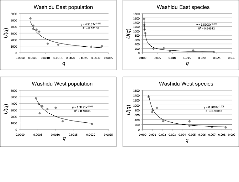
Figure 2: $U(q_{s})$ for Dictyostelia fitted with power functions.

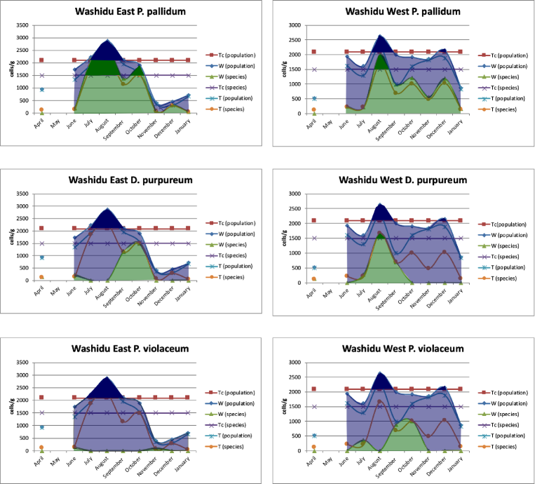
Figure 3: $W/T_{c}/T_{s}$ dynamics. P. pallidum: Polysphondylium pallidum; D. purpureum: Dictyostelium purpureum; P. violaceum: Polysphondylium violaceum. Dark blue shading indicates a phase in which the given population dominates; light blue indicates a phase in which a population is increasing; dark green indicates a particular species dominates; and light green indicates that a particular species is increasing. Populations include all species within the system, and are thus not restricted to the species labeled at the top of each figure.

Furthermore, $T_{s}<T_{c}$ increases the internal energy,

$$E(T_{s})=-\bar{N}h\tanh(q_{s}h)\approx-\bar{N}q_{s}h^{2},$$ (69)

when $\bar{N}$ is $N_{k}$ averaged over patches in populations or species. When $T_{s}>T_{c}$, $E=0$, and when $T_{s}<T_{c}$, $E$ is proportional to $T_{c}-T_{s}$. The specific heat $C_{s}(=\partial E/\partial T_{s}|_{h=0})$ is $0$ at or above $T_{c}$, it is finite at or below the $T_{c}$, and it has a sudden increase at $T_{c}$. Usually, species have higher internal energy than do populations. The critical point can be determined by using data specific to a given species; note that there are several phases for population and species, including domination, increasing, and chaos.

2.9 Introducing large S, an order parameter

For the population space defined above and the volume of the system $V=1$ for 1 gram of soil, we define $S$ near the critical points as follows:

$$f\{S\}=f_{0}+A^{\prime}S^{2}+B^{\prime}S^{4}-h^{\prime}S,$$ (70)

where $f=F\approx G$ is the Hamiltonian; $h^{\prime}$ is the flow of the population from outside; and $f_{0}$, $A^{\prime}$, and $B^{\prime}$ are coefficients approximated by an expansion and assuming $B^{\prime}>0$ and $A^{\prime}=A^{\prime\prime}(T_{s}-T_{c})$, in which $A^{\prime\prime}$ is another approximated coefficient. At equilibrium,

$$\frac{\partial f}{\partial S}=4B^{\prime}S^{3}+2A^{\prime\prime}(T_{s}-T_{c})S-h^{\prime}=0,$$ (71)

and the solution is the order parameter. When $h^{\prime}=0$, $S=0$ is the only solution of $T_{s}>T_{c}$. An additional solution, $S\approx\pm(T_{c}-T_{s})^{1/2}$, exists when $T_{s}<T_{c}$, with $h^{\prime}$ breaking the symmetry. The isothermal susceptibility is $\chi_{T}\approx|T_{s}-T_{c}|^{-1}$. When $T_{s}=T_{c}$, we have $S\approx h^{\prime 1/3}$. When $C_{0}=-T_{s}\partial^{2}f_{0}/\partial T_{s}^{2}$, we have the specific heat $C_{s}=C_{0}$ at $T_{s}>T_{c}$, $C_{s}=T_{s}A^{\prime\prime 2}/2B^{\prime}$ at $T_{s}<T_{c}$, and a jump at $T_{s}=T_{c}$. The calculated values of $S$ are listed in Table 4. The results indicate that there is a tendency towards order when a population or species dominates.

2.10 Application of the type IV Painlevé equation to an $X^{2}$ system

After the dicussion in equilibrium, We will now discuss the development of time-related function $t$ (time is actually $t^{2}$) in our system. Assume that $X^{2},XY,Y^{2}$ (instead of $X,Y$, as modeling the selection of the interactions among $X,Y$; that is, $X^{2},Y^{2}$ correspond to $N_{X},N_{Y}$ and $XY$ is a term of interaction) obey the Lotka-Volterra equations, which are equivalent to the type IV Painlevé equations:

$$\frac{dX^{2}}{dt}=X^{2}(XY-Y^{2}),\frac{dXY}{dt}=-XY(X^{2}+Y^{2}),\frac{dY^{2}}{dt}=Y^{2}(XY-X^{2}).$$ (72)

The system represents the adaptive species situation discussed in the previous subsection and has the required symmetry. If the second equation is converted to $\frac{dXY}{dt}=XY(X^{2}+Y^{2})$, then the system becomes cooperative. To obtain $\dot{X}$, simply divide the equation by $2X$. Now let us consider $N_{P}(t)=1/X$. We apply the Verhulst logistic equation model proposed by [Lizama and Mesquita, 2013]:

$$\frac{dN_{P}(t)}{dt}=N_{P}(t)(a_{P}(t)-b_{P}(t)N_{P}(t)).$$ (73)

Therefore, $a_{P}(t)=-XY/2$, $b_{P}(t)=-XY^{2}/2$, and if we set $c_{P}(t)=e^{Y}$,

$$N_{P}(t+1)=N_{P}(t)^{\frac{1}{1+\frac{1}{b}}}c_{P}(t)^{\frac{1}{b(1+\frac{1}{b})}},$$ (74)

and $t=b\arg D$ is properly selected. Note that a gauge function $h_{t}(t_{t})$ will be $(\ln t_{t}^{-1})^{m_{h}-1}$ where $t_{t}=e^{-\frac{1}{b}}$ and $m_{h}=\Re(s)$ [Lapidus et al., 2017]. From this, it is clear that the root of time is proportional to the temperature $b$ of $N_{k}=a-b\ln k$ (not $b(t)$ in the above equation), and the inverse temperature is related to the root of generation time, which is the inverse of $t$. Next, consider an absolute zeta function

$$\zeta_{\mathbb{G}_{m}/F_{1}}(s)=\frac{s}{s-1}=\frac{s}{w},$$ (75)

when $\mathbb{G}_{m}=GL(1)$. Note that $s/w$ is the value of $s$ for a particular group during the previous time step. Therefore, $\arg w=\arg D=1/b$ (time and $\arg D$ are measured in opposite directions). If we consider $\mathbb{G}:\mathbb{H}$/|H|$\times\mathbb{R}\times\mathbb{R}$ in terms of introducing $\Im(s)$ to explain adaptation/disadaptation of a species, there is a unique irreducible unitary representation $\rho_{G}:\mathbb{G}\rightarrow GL(W)$, besides an isomorphism, and for any $c_{G}\in\mathbb{H}$/|H|,

$$\rho_{G}(c_{G})=c_{G}\mathrm{Id}_{W}$$ (76)

when $\mathrm{Id}_{W}$ is an identity mapping (Stone-von Neumann theorem; [Stone, 1930] [von Neumann, 1931] [von Neumann, 1932] [Stone, 1932]). This representation characterizes the system, which is still not possible at this moment.

Let us further expand this approach. Consider the Gauss equation with rational $\alpha,\beta,\gamma$:

$$t(1-t)y^{\prime\prime}+\{\gamma-(\alpha+\beta+1)t\}y^{\prime}-\alpha\beta y=0.$$ (77)

If we select a quotient of two linearly independent solutions of the equation, $w_{y}(t)=y_{1}/y_{2}$, the Schwarz equation is

$$(\frac{w_{y}^{\prime\prime}}{w_{y}^{\prime}})^{\prime}-\frac{1}{2}(\frac{w_{y}^{\prime\prime}}{w_{y}^{\prime}})^{2}=\frac{1}{2}(\frac{1-\lambda^{2}}{t^{2}}+\frac{1-\mu^{2}}{(t-1)^{2}}+\frac{\lambda^{2}+\mu^{2}-\nu^{2}-1}{t(t-1)})$$ (78)

when $\lambda^{2}=(1-\gamma)^{2},\mu^{2}=(\gamma-\alpha-\beta)^{2}$, and $\nu^{2}=(\alpha-\beta)^{2}$. Next, consider $y=D$. When $b\neq 0$, the branch points of $w_{y}$: $t=0,1,\infty$ are $\arg D=0,1/b,\infty$, respectively. Since $\arg D$ should be $\lambda\pi,\mu\pi,\nu\pi$, respectively, we obtain $\gamma=1$ and $\gamma-\alpha-\beta=\pm 1/(b\pi)$. Therefore,

$$w_{y}^{\prime}=\frac{y_{1}}{y_{2}}=\frac{constance\ t^{-\gamma}(t-1)^{\gamma-\alpha-\beta-1}}{y_{2}^{2}}=\frac{constance\ t^{-1}(t-1)^{\pm\frac{1}{b\pi}-1}}{y_{2}^{2}},$$ (79)

and $y_{1}=y_{2}=D$ results in

$$D=\pm\sqrt{\frac{constance}{t(t-1)^{1\mp\frac{1}{b\pi}}}}.$$ (80)

Assuming $t$ proceeds in the negative direction (because $D>1$),

$$D_{t-1}=\sqrt{(t-1)^{\mp\frac{1}{b_{t}\pi}}\frac{t}{(t-2)^{1\mp\frac{1}{b_{t-1}\pi}}}}D_{t}$$ (81)

when $t\neq 0,1,\infty$ (double-signs correspond). Thus,

$$D=\Biggl{\{}(t-1)^{\mp\frac{1}{b_{t}\pi}}\frac{t}{(t-2)^{1\mp\frac{1}{b_{t-1}\pi}}}\Biggr{\}}^{\frac{1}{2t}}.$$ (82)

For $t=0,1,\infty$, consider the Gauss hypergeometric function:

$$F_{G}(a_{F},b_{F},c_{F};z_{F})=\frac{\Gamma(c_{F})}{\Gamma(a_{F})\Gamma(c_{F}-a_{F})}\int_{0}^{1}t_{F}^{a_{F}-1}(1-t_{F})^{c_{F}-a_{F}-1}(1-t_{F}z_{F})^{-b_{F}}dt_{F}.$$ (83)

The solutions for $t=0$ are

$$y_{1,0}=F_{G}(\alpha,\beta,\gamma;t)=\infty,$$ (84)

$$y_{2,0}=t^{1-\gamma}F_{G}(\alpha-\gamma+1,\beta-\gamma+1,2-\gamma;t)=\infty.$$ (85)

The solutions for $t=1$ are

$$y_{1,1}=F_{G}(\alpha,\beta,\alpha+\beta-\gamma+1;1-t)=\infty,$$ (86)

$$y_{2,1}=(1-t)^{\gamma-\alpha-\beta}F_{G}(\gamma-\alpha,\gamma-\beta,\gamma-\alpha-\beta+1;1-t)=\infty.$$ (87)

These solutions arise from the assumptions of our biological model. The actual converged values of $D$, including $t=2$, should be validated either by observation or by calculation from other time points. The solutions for $t=\infty$ are

$$y_{1,\infty}=t^{-\alpha}F_{G}(\alpha,\alpha+1-\gamma,\alpha-\beta+1;1/t)=0,$$ (88)

$$y_{2,\infty}=t^{-\beta}F_{G}(\beta,\beta+1-\gamma,\beta-\alpha+1;1/t)=\infty,$$ (89)

as expected. For the purposes of model validation, we neglect the values from populations because $t$ is usually close to 1 or 2, indicating the values are not converging (chaos). Setting $b_{t}\sim b_{t-1}$ when $t>>1$, we examined 21 calculable values of species and omitted three values (October for Washidu West D. purpureum, $N=0$; August for Washidu West P. violaceum, $N=0$; and September for Washidu West P. violaceum, $\Re(s)=0.32$, which is too small); the observed/expected $D$ values are shown in Figure 4. A Student’s $t$ test indicated that our model was a good fit to the observations ($p=0.809$). Pearson’s $\chi^{2}$ similarly indicated the extent of the match ($\chi^{2}=1.281$, $p=1.000$).

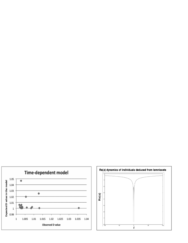
Figure 4: Plots of observed and expected $D$ values in the time-dependent model, and individual $\Re(s)_{l}$dynamics from the lemniscate.

For population-level dynamics, it is difficult to predict outputs directly because of the chaotic situation. However, we can introduce a newly defined $\Re(s)_{l}$ as follows. Consider a lemniscate function of

$$r^{2}=2a_{l}^{2}\cos 2\theta,\arg D=r=\frac{1}{b}t,a_{l}=\frac{1}{b}.$$ (90)

We can set an almost confluent situation of individual population growth with $b\sim 1$ and $E(\Sigma N)\sim 1$. Since $\theta=\arg\arg D=2\pi e^{Re(s)_{l}}$,

$$\Re(s)_{l}=\ln\{\frac{\arccos(\frac{1}{2}t^{2})}{4\pi}\}.$$ (91)

The values among populations are likely to be negative. From these calculations, we can estimate the overall trend of the growth/decline of a metapopulation; see the right panel in Figure 4.

2.11 Development of the model by web-based formalism

Here, we introduce an analogy to supersymmetry to further describe the time development of our model. This is Hodge-Kodaira decomposition for $\phi$ function:

$$I\phi^{j}(\Re(s))=\underset{p_{s}+q_{s}=j}{\bigoplus}I\phi^{p_{s},q_{s}}(\Re(s)),(\overline{\phi^{p_{s},q_{s}}(\Re(s))}=\phi^{q_{s},p_{s}}(\Re(s))=\phi^{p_{s},q_{s}}(-\Re(s)),$$ (92)

where $I:\phi\to v=\ln N_{k}/\ln\Im(s)$ for cohomology group as in [Adachi, 2017].

First, consider Bochner’s conjecture: for $\phi$ to be a characteristic function of the probability, the following three conditions are both necessary and sufficient: (I) $|\phi|/2$ is a positive constant; (II) $|\phi(\Re(s))|/2$ is continuous when $\Re(s)=0$; (III) $|\phi(0)|/2=1$. Therefore, $\phi(-\Re(s))=\overline{\phi(\Re(s))}$. Next, we consider the transactional interpretation of quantum physics [Cramer, 1986], or Hodge-Kodaira decomposition to explain the time symmetry of our model. Based on this, we develop a supersymmetry matrix:

$$\frac{1}{2}\left(\begin{array}[]{cc}\mathrm{F4}:\phi(\Re(s))&\mathrm{F1}:\overline{\phi(-\Re(s))}\\ \mathrm{F2}:-\phi(-\Re(s))&\mathrm{F3}:\overline{\phi(\Re(s))}\\ \end{array}\right),$$

where combinations of F4/F1 and F3/F2 are advanced/retarded waves and the determinant $\frac{1}{2}$(F4F3-F1F2) is past–future. Here, $\phi(\Re(s))$/$\overline{\phi(-\Re(s))}$ is the absorber/observer, and $-\phi(-\Re(s))$/$\overline{\phi(\Re(s))}$ is the emitter/observant; note that $\overline{\phi(\Re(s))}$ is the past and $-\phi(-\Re(s))$ is the future. In a complex-based system, the ($-1+i$)-adic system can be used to represent all complex numbers, whereas the ($1-i$)-adic system cannot [Knuth, 1997]. Moreover, when $n$ is natural, only $-n\pm i$ can be used to represent all complex numbers. Thus, F1 of the observer represents the information of all possible futures, while the observed F4 cannot represent all possibilities; this results in an asymmetry between the past and future. Although all scenarios may have been part of the past, the future is restricted to a particular scenario. In the same way, F2 cannot represent all possibilities, but F3 can. This is the opposite of the relationship between the observant and observer.

To expand this interpretation, consider [advanced–retarded] waves as a realization of the future population, $\mathrm{F4}-\mathrm{F1}$ and $\mathrm{F3}-\mathrm{F2}$, in the $(\pm 1\pm i)$-adic system. $\mathrm{F4}-\mathrm{F1}$ represents a population increase, and $\mathrm{F3}-\mathrm{F2}$ represents a population decrease. Their geometric mean is $2\sqrt{(\cos\theta+i\sin\theta)(\cos\theta-i\sin\theta)}=2$. Recall that bosons and fermions are orthogonal, based on the difference in their argument $\pi/2$, as in previous sections. The expected integral of this function is

$$\int_{0}^{\frac{\pi}{2}}\frac{d\theta}{2\sqrt{(\cos\theta+i\sin\theta)(\cos\theta-i\sin\theta)}}=\frac{\pi}{4}.$$ (93)

Remember that for an individual, the argument should be $\pi/4$, and an individual cannot represent the whole in the $(+1+i)$-adic system. To represent the whole, it is necessary to use a three-dimensional $(-1+i)$-adic system with an argument of $3\pi/4$, such as $X^{2},XY$, and $Y^{2}$. For example, consider

$$2\int_{-1}^{1}\sqrt{1-x^{2}}dx=2\int_{-1}^{1}\sqrt{(1+i\sqrt{x})(1-i\sqrt{x})(1+i\sqrt{-x})(1-i\sqrt{-x})}dx=\pi.$$ (94)

The integral over population changes from $-1$ (decrease) to +1 (increase) of the geometric mean of probabilities of the potential in $(population\ increase\ probability)^{2}$ with past and future (correspond to $1+i\sqrt{\pm x}$) and $(population\ decrease\ probability)^{2}$ with past and future (correspond to $1-i\sqrt{\pm x}$) results in $\pi/2$. Therefore, the expected value of the concomitant increase/decrease of two interactants is expected to be $\pi/2(<2)$. Similarly,

$$\int_{-1}^{1}\frac{dx}{\sqrt{1-x^{2}}}dx=\int_{-1}^{1}\frac{dx}{\sqrt{(1+i\sqrt{x})(1-i\sqrt{x})(1+i\sqrt{-x})(1-i\sqrt{-x})}}=\pi.$$ (95)

Therefore, the number of interacting dimensions (reciprocal of the expected probability) of the $\pm 1$ fluctuation is close to three. Furthermore,

$$\int_{-\infty}^{+\infty}\frac{dx}{1+x^{2}}=\int_{-\infty}^{\infty}\frac{dx}{(1+ix)(1-ix)}=\pi.$$ (96)

Considering all the potentials of a particular wave function, the expected dimensions should be close to three. In other words, the dimensionality of the F3 potential is equal to that of the F4 potential + $2\pi x$.

The above system of matrices is obviously $SU(2)$. Since the system is also a Kähler manifold without $s=1$, the four-dimensional Riemann manifold of the system becomes a Ricci-flat Kähler manifold/Calabi-Yau manifold [Kobayashi and Nomizu, 1996]. The system also has Riemann curvature tensors with self-duality, since it is a two-dimensional Ising model [Tasaki and Hara, 2015]. Furthermore, it is assumed to be asymptotically locally flat, and therefore the $\phi$ space is an instanton. If we set $\overline{W_{z}}$, where a superpotential $W_{z}=\phi\frac{N_{k}+1}{N_{k}}(\Phi-e^{-iN\vartheta}\frac{\Phi^{N_{k}+1}}{N_{k}+1})$ for $\Phi=\phi i$, this is analogous to the $\phi-instanton\ equation$ described by [Gaiotto et al., 2016]:

$$(\frac{\partial}{\partial x}+i\frac{\partial}{\partial\tau})\Phi^{I}=\frac{i\phi}{2}g^{I\overline{J}}\frac{\partial\overline{W_{z}}}{\partial\overline{\Phi}^{\overline{J}}},$$ (97)

where $x$ is the genetic information, $\tau$ is time, $g^{I\overline{J}}$ is a metric tensor, and $\Re(\phi^{-1}W_{z})$ and $\Im(\phi^{-1}W_{z})$ are the Hamiltonian and the potential of the system, respectively. Assuming the unified neutral theory, $\Phi$ itself is a quantum critical point. This is because within the population system, it is assumed to be in equilibrium with the highest adaptation in the ordered state, and the lowest value of the critical temperature is $T_{qc}=0$. Thus, each individual in the population has an equal role. With a vacuum weight $v_{ij}=v_{i}-v_{j}$, where $v_{i}=\phi\overline{W_{z}}_{i}$, the worldline is parallel to $v_{ij}$. The vacuum configurations $\Phi_{i}$ and $\Phi_{j}$ exhibit a boundary for each critical point/state. When $e^{i\theta}\frac{W_{ji}}{|W_{ji}|}=\phi$, $\Phi_{i}$ is a boosted soliton of the stationary soliton $\Phi_{j}$, and these define the edges of the webs [Gaiotto et al., 2016].

2.12 Implications of the model as a nine-dimensional system

When $|N(p)|$ is 1 or 2/3, this suggests that the model described here has $\mathcal{N}=2$ supersymmetry with three dimensions. In the previous subsection, we included supersymmetry, and in this subsection, we include three-dimensionality in the model. The equation that we need was presented in [Károlyházy, 1966]; this is the original work, which contained a serious misprint; for corrections and details, see [Károlyházy et al., 1986]:

$$(\Delta\Phi)^{2}\approx\Lambda^{4/3}\Phi^{2/3}.$$ (98)

To apply this equation, we need an analogue to the speed of light and to the uncertainty principle. For the speed of light, recall that

$$\frac{\partial\Re(s)}{\partial t}=b\frac{1}{|D|}\frac{\partial|D|}{\partial t}.$$ (99)

This is analogous to Hubble’s law for $H(t)$:

$$\frac{dD}{dt}=H(t)D,$$ (100)

with

$$\frac{\partial\Re(s)}{\partial t}=bH(t).$$ (101)

Note that $\max(dD/dt)=|D|^{E(\Sigma N)}$ for the observed system. The parameter analogous to the speed of light is therefore $|D|^{E(\Sigma N)}$. If we consider the time-dependent function $D$ considered in the previous sections, then we have

$$H(t)=\frac{1}{D}\frac{dD}{dt}=\frac{t^{2}-4t+2}{2t^{2}(t-1)(t-2)}-\frac{1}{2t^{2}}\ln[\{(t-1)^{\mp\frac{1}{b_{t}\pi}}\frac{t}{(t-2)^{1\mp\frac{1}{b_{t-1}\pi}}}\}].$$ (102)

The uncertainty principle can be written as $\Delta D\Delta p_{m}\geq\hbar/2$, where $p_{m}=M_{mass}\dot{D}$. We can set $\hbar=1$. If we set $M_{mass}=H(t)^{-1}=\phi\approx constant$ and $D=1+\Delta N_{k}$, then the uncertainty principle simplifies to $(\Delta\Delta N_{k})^{2}\geq 1$; obviously, this condition is fulfilled by the system by changing $D$. Since $|dD/dt|=|D|^{E(\Sigma N)}$ is only achieved when $\phi=0$, the condition for the analogy to the photon is appropriate.

Now, let $|\Phi|=N_{k}/E(\Sigma N)\propto T_{s}$ in equilibrium. If $G$ is an analogue of the gravitational constant, the Planck scale can be written as $\Lambda=\sqrt{\hbar G/|D|^{3E(\Sigma N)}}$. When $\phi_{i}$ is the mass of the internal populations and $\phi_{e}$ is that from the external populations, we can set $V_{p}=GM_{i}M_{e}/D\approx\phi_{i}$. Note that $G=D/\phi_{e}=1/(\phi_{e}-\Delta\phi_{e})\approx constant$ ($\phi/D=PD^{N_{k}-1}=\phi-\Delta\phi$), and $\Lambda^{2}\approx constant$. Therefore $(\Delta\Phi)^{3}\propto\Phi$, that is, $\Phi$ is the third power of its fluctuation, assuming $D^{E(\Sigma N)}=constant$. If we apply $\mathcal{N}=2$ supersymmetry with the three-dimensional Ising model [Bobev et al., 2015], then the kink is $\bigtriangleup=|N(p)|=2/3$ and the superpotential is $\mathbf{W}=\Phi^{3}$. The dimensionality of the Ising model should be three. Next, we consider the Stefan-Boltzmann law. Since the entropy density is $s_{d}=4U/3T_{s}\propto T_{s}^{3}$, there are nine dimensions in $s_{d}\propto\mathbf{W}$; this is similar to the case in superstring theory. Note that $\mathbf{W}$ and $s_{d}$ are in opposite directions. We can also set a three-dimensional fermionic Grassmann number, similar to what we did with string theory, if we assume a zero-sum patch game of the unified neutral theory and assume the fitness is $w$. The future predicted by the model is the Eisenstein series with $w_{Q}=3$ [Marinõ, 2014]. Overall, based on the requirements from $\mathbf{W}=\Phi^{3}$ and $w_{Q}=3$, $w_{Q}$ should be $3$ and $|N(p)|=1$ should be in the interacting mode.

Additionally, according to [Steinhardt and Turok, 2004], for a universe with constant $\epsilon$, the scale factor $a(t)$ and the Hubble radius $H(t)^{-1}$ are related by the Friedmann equations with our modification of the $t\rightarrow t^{2}$ correspondence in $H(t)$ (that is, time emerges from a self-interaction of a particular potential $\Im(s)$):

$$a(t)\approx t^{2/\epsilon}\approx(H(t)^{-1})^{1/\epsilon}.$$ (103)

Let us set $\epsilon\equiv 3/2*(1+\varpi)$. In this system, $\varpi>1$, $-1/3<\varpi\leq 1$, and $\varpi\leq-1/3$ correspond to contraction, oscillation, and expansion of the universe. Since $\epsilon=1/\bigtriangleup$, $|N(p)|=1,2/3$ show expansion/oscillation of the universe. Therefore, the former mode represents expansion, and it turns into the latter mode with oscillation, not with expansion. We need further development of new dimension as a result of multilevel selection to expand another higher level of hierarchy.

2.13 Induction of hierarchy and time through one-dimensional probability space with certain topologies

It appears doubtful why single-dimensional information ($N_{k}$), with a topology labelled by rank $k$, can induce a 3-dimensional system ($a,b,\ln k$, regarding $N_{k}$ as free energy, the others as internal energy or enthalpy, temperature, and entropy, respectively) of an individual density, accompanied with an even additional time dimension. To explain this, first of all, we set a $1$-dimensional $C^{\infty}$ manifold with a topology as $(B,\mathscr{O})$ with $s\in B$. Inspired by the Bethe ansatz (e.g. [Bethe, 1931]), we set three different topologies isomorphic to $\Delta,\mathbb{C},\hat{\mathbb{C}}$ for further clarification of our model. These topologies naturally invest a cohomology, time dimension, and hierarchy to the system. Furthermore, we are able to define a proper topology independently from moduli of measurements with individual numbers and a Galois action dependent on moduli of it in an evolutionary system with hierarchy by Galois extension, such as biological systems in this case. For application to biological hierarchies, this model is tested using protein abundance data derived from liquid-chromatography mass spectrometry (LC/MS) of HEK-293 cells and species density data from a wild Dictyostelia community. Finally, we sought to evaluate interactions of the constituents of biological systems by invoking a Weierstraß $\wp$ function to estimate the strength of homo- and hetero-interactions. These results serve to further justify our “small $s$” metric to decipher system dynamics of interest. For example, adapted, non-adapted (neutral), and disadapted (repressed) proteins can be classified by expansion of the model using a Clifford algebra. Furthermore, utilizing a congruent zeta function elucidates the contribution to adaptive/disadaptive situations from each hierarchy.

2.14 General guidelines for topological evaluations

We start from a 1-dimensional $C^{\infty}$ manifold with a topology, $(B,\mathscr{O})$. Note that many aspects of $(B,\mathscr{O})$ can be explained by the inverse square law by drawing on forces in the models below.

This partial topology of $\mathscr{O}$ means, for example, a regular automorphism on $\Delta$, $f(\Delta)=\{e^{i\theta}\frac{z-\alpha}{1-\bar{\alpha}z};z\in B,\theta\in\mathbb{R},\alpha\in\Delta\}$ can explain anything emanating from the set of $f$, for example, isomorphism to $\mathbb{R}^{3}$ space, and explored in more detail below. An apparently neutral particle system introduced with hierarchies by Galois extension could be $\mathrm{Gal}(\mathbb{Q}(\zeta_{n})/\mathbb{Q})\cong(\mathbb{Z}/n\mathbb{Z})^{\times}$ when $\zeta_{n}$ is a cyclotomic field. If GCD$(n,m)$ is $1$, $\mathrm{Gal}(\mathbb{Q}(\zeta_{nm})/\mathbb{Q})\cong\mathrm{Gal}(\mathbb{Q}(\zeta_{n})/\mathbb{Q})\times\mathrm{Gal}(\mathbb{Q}(\zeta_{m})/\mathbb{Q})$. This would lead to a Kummer extension decomposed to species with $p$ identity.

For a topology of $\mathbb{C}$, $f(\mathbb{C})=\{az+b;z\in B,a,b\in\mathbb{C}\}$ and isomorphic to $\mathbb{R}^{4}$, later indicated as ($3+1$) dimensions with a time dimension. Obviously interaction of a complex metric, e.g. $s^{2},w^{2}$ can induce a time dimension. For a topology of $\hat{\mathbb{C}}$, $f(\hat{\mathbb{C}})=\{\frac{az+b}{cz+d};z\in B,a,b,c,d\in\mathbb{C}\}$ and isomorphic to $\mathbb{R}^{6}(\mathbb{R}^{3}\times\mathbb{R}^{3})$, later indicated by letting $\mathbb{R}^{4}$ compact by inducing a hierarchy.

Fundamentally, a simply connected subregion without holes such as a Riemann surface induced during hierarchization is isomorphic and holomorphic to either $\Delta,\mathbb{C}$, or $\hat{\mathbb{C}}$. Schwarz-Christoffel mapping enables a conformal transformation from polygons to one of those regions, and the Widely Applicable Information Criterion (WAIC) has a central role as an analogy to logarithmic velocity in fluid mechanics calculated from $D$. Without singularity, this is straightforward to consider and we focus on the case for singular points. As in the Bethe ansatz [Bethe, 1931], a single dimension $z$ with a particular topology is able to induce both a ($3+1$)-dimensional system and hierarchies.

$\mathscr{O}\cong\Delta$ case

The Riemann-Roch theorem states

$$l(D)-l(K-D)=\mathrm{deg}(D)-g+1,$$ (104)

where $D$ is a divisor, $K$ is a canonical divisor, and $g$ is a genus number. Let $TB$ be a bundle. An interaction, $TB\tilde{\times}TB:=\bigcup_{p\in B}T_{p}B\times T_{p}B$, becomes a 3-dimensional $C^{\infty}$ manifold. Let open base elements of the manifold be $x,y,z$, and the planes on the bases be $X,Y,Z$. If we consider interactions of these bases, the left term of Eq. (101) is 3, from $g=10$ and $\mathrm{deg}(D)=12$.

Let $F$

$$F(z)=q\prod_{n=1}^{\infty}(1-q^{n})^{2}(1-q^{11n})^{2}=\sum_{n=1}^{\infty}c(n)q^{n}$$ (105)

be a totally real number field of degree $g$ over $\mathbb{Q}$, and $\mathbb{K}$ be a totally imaginary quartic extension of $F$. Let $D$ and $D^{int}$ be simple algebras over $\mathbb{K}$ with $D=e^{s/b}$. Let $\mathbf{G}=\mathbf{GU}(D,\alpha)$ with $\alpha$ being a second kind involution of $D$. Take a 3-dimensional $\ell$-adic system in which $W_{E}=\Re(s)=\ell,D^{\times}=p=|D|^{E(\Sigma N)},GL_{d}(E)=v=\ln N_{k}/\ln p$, where $W_{E}$ denotes the Weil group of center $E$ as a Langlands correspondence [Rapoport and Zink, 1996] [Adachi, 2017]. $\ell$ is obviously an étale (crystalline) topology independent of moduli $N_{k}$, in the sense that a homomorphism of Noetherian local rings is unramified and flat, and the object is a localization of a finitely generated algebra of the origin. These $p$($\ell$)-adic geometries are analogical to real differentiables and Clifford-Klein geometries as calculated later. The $\mathscr{O}\cong\Delta$ case visualizes both persistence homology $p$ and étale cohomology $l$.

$\mathscr{O}\cong\mathbb{C}$ case

A Minkowski metric small $s$ can be utilized for a time developing model when $\sin,\cos$ of the metric are converted to $\sinh,\cosh$. However, for more detailed analysis, another Minkowski metric in our model could be

$$s_{M}=[\Im(s)^{2}(\Delta\Im(s))^{2}-(\Delta a)^{2}-(\Delta b)^{2}-(\Delta\ln k)^{2}]^{\frac{1}{2}}.$$ (106)

In this sense, the world line of a species is identical and a different species is non-zero, discretely depending on $\Delta\Im(s)$. When we take $ds_{M}^{2}=a(V_{1})ds_{M1}^{2},ds_{M1}^{2}=a(V_{2})ds_{M2}^{2}$, and so on. $ds_{M}^{2}=ds_{M}^{\prime 2}$ due to a Lorentz transformation and $\ln(s_{M})=\sum_{i=1}^{\infty}\ln a(V_{i})$ becomes a module when $2ds_{M}=0$. A set of species can thus be characterized by this module of $s_{M}$. A Lagrangian could be

$$L=-\phi\Im(s),$$ (107)

and a Hamiltonian could be

$$\mathscr{H}=-\phi\Im(s)^{2}\sqrt{\frac{\Im(s)^{2}+(H(t)D)^{2}}{\Im(s)^{2}-(H(t)D)^{2}}}.$$ (108)

We can consider $D^{\prime}\cong D^{int}$, $\mathbf{G}^{\prime}\cong\mathbf{G^{int}}$, and a time dimension is induced by some admissible isomorphisms (Proposition 2.5.6 in [Varshavsky, 1998]). Note that ‘temperature’ $b$ and root of time $t$ are closely correlated by $t=b\arg D$. Now consider the $\mathrm{Poincar\acute{e}}$ conjecture, where every simply connected closed $n$-dimensional manifold $W_{E}$ is homeomorphic to $n$-dimensional sphere $S^{n}$. Let a Morse function be $f:W_{E}\rightarrow[a,b]$, in which $a,b$ are regular values. Let $f$ have critical points $p,p^{\prime}$ that correspond to indexes $\lambda,\lambda+1$ as time. Consider that $S^{n-\lambda-1}$ and $S^{\lambda}$ cross at a single point; this indicates the status of present. The exchange of Morse functions would result in no new critical point appearing and disappearance of critical points $p,p^{\prime}$ ($h$-cobordism theorem). This is what happens at the present state following the time arrow. Remark that $p,p^{\prime}$ are linked to a Hecke ring via non-trivial zero points of Riemann zeta, fulfilling the condition of the Yang-Baxter equation. Thus this phenomenon is closely related to an analogy to quantum entanglement and face models [Baxter, 1973] [Andrews et al., 1984]. Of course, in the case of species, as species still exist, they will reappear with different $p$ values in this model.

In this sense, for any labelling of time points $\tau^{\prime}\in\mathcal{T}_{S^{*}}$, a potential for the Petersson-Weil metric is as follows:

$$\omega_{WP}=d(\sigma_{\mathcal{T}}(\tau\mathrel{\vee\!\!\!\!\bot}\tau*)-\sigma_{\mathcal{T}}(\tau\mathrel{\vee\!\!\!\!\bot}\tau^{\prime})),$$ (109)

when $\mathrel{\vee\!\!\!\!\bot}$ is a quasi-Fuchsian Kleinian group [Hubbard, 2006]. The ‘mating’ represents the coupling of times corresponding to $p,p^{\prime}$.

Now consider $p$, $p^{\prime}$ as characteristics on a field $k$, as in $d=p=0$ in [Adachi, 2017]. Let $E$ be a singular hyperelliptic curve of the system. Real $D$ will be a tensor product of an endomorphism of $E$ on $\bar{k}$ and $\mathbb{Q}$, approximately. The resultant $D$ is a quaternion field on $\mathbb{Q}$. Take a set of $\ln N$ as an $\ell$-adic rational Tate module as in [Adachi, 2017]. $D$ will only ramify at $p,p^{\prime}$ or a point at infinity (c.f. [Silverman, 1986]). This restricts the possible direction of the time arrow to vanish $p,p^{\prime}$ only.

Generally, for species, we draw a picture of time development when the observer is at $k=1$. For other observations, we can simply take $k\to k^{\prime}$ shifts for the calculations. That is, we can take a cyclotomic field related to the number of $k_{\mathrm{max}}$. In this sense, time in the context of a complex metric can be utilized and the world line is in web form branched at each cross-section of $p$ and $p^{\prime}$, not in parallel as discussed in some studies. For moving one distinct world line to another, we need velocity $H(t)D>\Im(s)$.

Next, shift from $p$ to $l=\Re(s)$ following the method outlined, and simply consider a combinatory function in a probability space, $\Gamma(s+1)=s\Gamma(s)$. This is an example of a shift map. If we take a function similar to a $\Gamma$ function, we can observe discrete time development merely by multiplying a master $s$ function if we know the particular $s$. That is, adding a single fractal dimension in the past world (subtracting a single dimension from the future world by an observation) results in a simple multiplication of $s$ and master $\Gamma(s)$. Therefore, only evaluating an $s$ of interest is sufficient for this aim.

Similarly, consider the Maass form of the Selberg zeta function as calculating the mode of species dynamics. Stirling’s approximation would be $\Gamma(s)\approx\sqrt{\frac{2\pi}{s}}(\frac{s}{e})^{s}\exp(\frac{1}{12s})$, and considering a first-order approximation of the exponent with $(1+1/12s)$ can suitably approximate the situation with superstring theory of $12$ dimensions. For further approximation, we need additional dimensions. Jacobian mapping independent of a path $\lambda$

$$\Phi(p)=(\int_{\lambda}\varphi_{1},\cdots,\int_{\lambda}\varphi_{g})\in\mathbb{C}^{g}/^{t}\Omega\mathbb{Z}^{2g}=\underset{\sim}{J}(B)$$ (110)

is one choice. If we know the master Maass form as the invariant form for $\rho_{G}(c_{G})=c_{G}\mathrm{Id}_{W}$ when $\mathrm{Id}_{W}$ is an identity mapping of a system of interest (Stone-von Neumann theorem; [Stone, 1930] [von Neumann, 1931] [von Neumann, 1932] [Stone, 1932]), differential operation does not cause any difference in the form. This ensures the condition for a suitable $\mathcal{D}$-module and the accompanying derived category. Thus we can adopt a modified microlocally analytic $b$ function as $\partial_{b}=i\partial$ as a substitute for the differential operation; i.e., $\partial_{b}^{2}=-\partial^{2}$, rotating the form in the angle of $\pi$, and $\partial_{b}^{4}=\partial^{4}=i.d.$, reverting back to the original orientation of the form. An Ornstein-Uhlenbeck operator would be $L=-\sum_{i=1}^{d}\partial_{i}^{*}\partial_{i}=\sum_{i=1}^{d}\partial_{b}^{2}$. Setting a bounded Baire function $h$ on $\mathbb{R}^{d}$ and $f$ as a solution of $Lf=h-<h>,<h>=\int_{\mathbb{R}^{d}}h(x)g(x)dx$, $E(h(W))-<h>=E(Lf(W))$ means a deviation from the expected function $h$ value in the future. The operator $\partial_{b}$ is thus characterized for an operator calculating a future state. $\partial_{b}^{2}$ could be an element of a $\mathcal{D}$-module as $\mathcal{D}\circ\mathcal{D}=i.d.$ Then $\partial_{b}$ would develop to analogies to energy or momentum, $\partial_{b}/\partial t=E$ or $-\partial_{b}/\partial x_{k}=p_{x_{k}}$ as variations of operators. The $\pi/2$ rotation of $\Im(s)$ is thus justified by the modified $b$ function. Considering $(3+1)$ dimensions with an interaction of two 2-dimensional particles, this theory and transactional interpretation of quantum mechanics [Cramer, 1986] are suitable. If we regard $\partial_{b}^{k},k\in\mathbb{Z}$ as ideals of a finitely generated Jacobson radical, Nakayama’s lemma shows maintaining identity before and after the operation means the module is zero. Therefore, in this finite case, everything is an observant and at least an infinite generation is required to achieve the values out of zeros. That means, if we see something, time is infinite. Hironaka’s resolution of singularities at characteristic $0$ implies such a mating of $p,p^{\prime}$.

To resolve such a master relation, consider a form of “velocity” as $v\in TB$. Then take a 2-dimensional space consisting of $s\in B$. $s(v,t)=p(v)+tq(v)$ as in a Lagrange equation. The Gauss curvature of this surface $K\leq 0$. $K\equiv 0$ is only achieved when $TB$ is time-independent, and this $TB$ with $K=0$ is the time-invariant bundle usable for $TB\tilde{\times}TB$ calculation for a 3-dimensional system and 6-dimensional hierarchies. Additionally, the Legendre transformation of the above equation is $X=v,Y=tv-s,Z=t$ and $\{v-q(v)\}\frac{dY}{dv}=Y+p(v)$. $K=0$ means $v=0$ and $s=p(0)$ is the required solution. Furthermore, $s$ can be regarded as a Dirac measure ($w$ is a counterpart of mass and $s=w+1$), and $s^{\prime}=-s$ can be regarded as a Schwartz distribution. Although addition is allowed in the distribution, generally multiplication is not (we will illustrate that it is feasible later). However, setting the differential as $\partial_{b}^{2}$, it becomes first order with a minus sign and differentiation by time: $t^{2}$ is plausible. For instance,

$$\begin{split}\int\int\underset{V}{\cdots}\int s\Delta\varphi dt=\int\int\underset{V}{\cdots}\int\varphi[\Delta s]dt+\int\underset{S}{\cdots}\int s[\frac{d\varphi}{d\nu}]dS\\ -\int\underset{S}{\cdots}\int\varphi[\frac{ds}{d\nu}]dS,\end{split}$$ (111)

where $\varphi$ is a distribution of interest, $s\in S$, and $\nu$ is a differential by unit area. The first term on the right is noise, the second is related to fractal structure, and the third is oscillative behavior. Besides singular points, it is regular. An entire function considering negative even singular points of $l-n$ regarding $w=s-1$ would be

$$Z_{l}=\frac{\mathrm{Pf.}w^{l-n}}{\pi^{(n-2)/2}2^{l-1}\Gamma(\frac{l}{2})\Gamma(\frac{l+2-n}{2})},$$ (112)

where at the singular points, $k\in\mathbb{Z}_{\geq 0},Z_{-2k}=\square^{k}w;\square=(-1)(\frac{\partial_{b}^{4}}{\partial x_{1}^{4}}+\frac{\partial_{b}^{4}}{\partial x_{2}^{4}}+\cdots+\frac{\partial_{b}^{4}}{\partial x_{n-1}^{4}}-\frac{\partial_{b}^{4}}{\partial t^{4}})$. In the $\varnothing=\partial B$ case, $\square Z_{2}=w,\square^{k}Z_{2k}=w$. This means, periodical population bursting/collapsing by negative even $w$ values. For negative odd $w$ values, chaos ensues (Šarkovski, Stefan, Block theorem) [Guckenheimer and Holmes, 1983]. Thus, adopting $s,w$ is suitable for applying a single-dimensional model. $s$ is a measure provided it is finite in bounded domains. Therefore, singular points reflect appearance/disappearance of fractal structures. In summary, a topology $\mathscr{O}$ should be $(\{m=k\}\subset\mathbb{N},\{\varepsilon=b\},\{\Omega=a\})$ of $N_{k}=a-b\ln k$. For further details regarding distributions, see [Schwartz, 1966].

Now let $E$ be an elliptic curve: $y^{2}+y=x^{3}-x^{2}$ as in [Eichler, 1954]. This is equivalent to $y(y+1)=x^{2}(x-1)$. If we consider ($3+1$)-dimensional $N=1\ SU(2)$ without fluctuation, $x^{2}$ could be mass, $(x-1)$ could be a goldstino as spontaneous breaking of supersymmetry, $y$ could be 3-dimensional fitness $D$ with fluctuation, and $y+1$ could be ($3+1$)-dimensional $s$. The goldstino would represent temporal asymmetry. In Gaussian ensembles, a complex system GUE breaks time-reversal and a self-dual quaternion system GSE preserves it. Therefore $y+1$ preserves time symmetry and consequently the present $y$ breaks the symmetry.

A Riemann scheme would uniformize the fitness space as a hypergeometric differential equation.

Now consider

$$\frac{dY}{dx}=(\frac{A}{x}+\frac{B}{x-1})Y,\\$$ (113)

$$A=\left(\begin{array}[]{ccc}\lambda_{1}+\lambda_{3}+\lambda_{4}+\lambda_{5}&\lambda_{2}&0\\ 0&\lambda_{3}+\lambda_{4}&\lambda_{5}\\ 0&0&0\end{array}\right),$$ (114)

$$B=\left(\begin{array}[]{ccc}0&0&0\\ 0&0&0\\ \frac{\lambda_{1}(\lambda_{1}+\lambda_{3}+\lambda_{5})}{\lambda_{5}}&\frac{\lambda_{1}\lambda_{2}+\lambda_{2}\lambda_{3}+\lambda_{3}\lambda_{5})}{\lambda_{5}}&\lambda_{2}+\lambda_{4}+\lambda_{5}\end{array}\right).$$ (115)

This will culminate in a generalized hypergeometric function ${}_{3}F_{2}$ that satisfies a Fuchs-type differential equation ${}_{3}E_{2}$. If we set proper region $\Delta$ (13 different regions),

$$y(x)=\int_{\Delta}s^{\lambda_{1}}(s-1)^{\lambda_{2}}t^{\lambda_{3}}(t-x)^{\lambda_{4}}(s-t)^{\lambda_{5}}dsdt.$$ (116)

$x=0$, $w=D$, $s=1$ would result in

$$y(0)=\int_{\Delta}s^{\lambda_{1}}w^{\lambda_{2}}t^{\lambda_{3}+\lambda_{4}}\{-(t-1)\}^{\lambda_{5}}dsdt.$$ (117)

$\lambda_{1}=\lambda_{2}=\lambda_{3}=\lambda_{4}=\lambda_{5}=1$ would be $E^{2}:-\int y(y+1)x^{2}(x-1)dxdy$ form, obviously the integral of the interaction of two elliptic curves.

For consideration of an interacting 4-dimensional system, let us take $\mathrm{Painlev\acute{e}}$ VI equations on a ($3+1$)-dimensional basis with a single Hamiltonian [Manin, 1999] [Kawakami et al., 2016]. The Hamiltonian should be $H_{k}=\partial_{k}\ln\tau(t)=\frac{\partial_{k}\tau(t)}{\tau(t)}=H(t)N_{k}=\frac{N_{k}}{E(\Sigma N)}=\phi$ when $H(t)$ is a Hubble parameter [Iorgov et al., 2015]. $\tau(t)$ is thus an inverse of a Hubble parameter, and its $k$th boundary is a $k$th species. Note that the 3-dimensional system represents the smallest possible number of dimensions whose associativity equations become non-empty even in the presence of the flat identity. Furthermore, considering a fundamental group $\pi_{1}$ of $C_{0,n}:=\mathbb{P}^{1}\backslash\{z_{1},...,z_{n}\}$, the dimension of representations $\rho$ of $\pi_{1}$ in $SL(2,\mathbb{C})$ is $2(n-3)$ [Iorgov et al., 2015]. If we would like to set $\pi_{1}$ as an $\mathrm{\acute{e}tale}$ topology with 0 dimension, $n=3$. ($3+1$)-dimensional semisimple Frobenius manifolds constitute a subfamily of $\mathrm{Painlev\acute{e}}$ VI:

$$\begin{split}\frac{d^{2}X}{dt^{2}}=\frac{1}{2}(\frac{1}{X}+\frac{1}{X-1}+\frac{1}{X-t})(\frac{dX}{dt})^{2}\\ -(\frac{1}{t}+\frac{1}{t-1}+\frac{1}{X-t})\frac{dX}{dt}\\ +\frac{X(X-1)(X-t)}{t^{2}(t-1)^{2}}[(\theta_{\infty}-\frac{1}{2})^{2}\\ +\theta_{0}^{2}\frac{t}{X^{2}}+\theta_{1}^{2}\frac{t-1}{(X-1)^{2}}+(\theta_{t}^{2}-\frac{1}{4})\frac{t(t-1)}{(X-t)^{2}}].\end{split}$$ (118)

Recall that the above equation is related to a rank 2 system:

$$\frac{d\Phi}{dz}=(\frac{\mathcal{A}_{0}}{z}+\frac{\mathcal{A}_{t}}{z-t}+\frac{\mathcal{A}_{1}}{z-1})\Phi,$$ (119)

or

$$\frac{d\mathcal{A}_{0}}{dt}=\frac{[\mathcal{A}_{t},\mathcal{A}_{0}]}{t},\frac{d\mathcal{A}_{1}}{dt}=\frac{[\mathcal{A}_{t},\mathcal{A}_{1}]}{t-1}$$ (120)

with 4 regular singular points $0,t,1,\infty$ on $\mathbb{P}_{1}$. Also,

$$\mathcal{A}_{0}+\mathcal{A}_{t}+\mathcal{A}_{1}=-\mathcal{A}_{\infty}=\mathrm{diag}\{-\theta_{\infty},\theta_{\infty}\}.$$ (121)

Note that the total sum of the matrix system is equal to 0. Assuming a 3-wave resonant system [Kakei and Kikuchi, 2007],

$$\partial_{\tau}u_{1}+c_{1}\partial_{x}u_{1}=i\gamma_{1}u_{2}^{*}u_{3}^{*}$$ (122)

$$\partial_{\tau}u_{2}+c_{2}\partial_{x}u_{2}=i\gamma_{2}u_{3}^{*}u_{1}^{*}$$ (123)

$$\partial_{\tau}u_{3}+c_{3}\partial_{x}u_{3}=i\gamma_{3}u_{1}^{*}u_{2}^{*}$$ (124)

An expansion of this model results in the $h_{V}^{11}=h_{\hat{V}}^{12}$ mirror symmetry relation for the Calabi-Yau threefolds. Recall that matrix $\mathrm{Painlev\acute{e}}$ systems of two interacting systems

$$\begin{split}t(t-1)H_{\mathrm{VI}}^{\mathrm{Mat}}(\alpha,\beta,\gamma,\delta,\omega;t;q_{1},p_{1},q_{2},p_{2})\\ =\mathrm{tr}[Q(Q-1)(Q-t)P^{2}\\ +\{(\delta-(\alpha-\omega)K)Q(Q-1)+\gamma(Q-1)(Q-t)\\ -(2\alpha+\beta+\gamma+\delta)Q(Q-t)\}P+\alpha(\alpha+\beta)Q],\end{split}$$ (125)

has 11 parameters.

Now let us convert a $\mathrm{Painlev\acute{e}}$ VI equation to a more realizable form as in physics. The $\mathrm{Painlev\acute{e}}$ VI equation is equivalent to

$$\frac{d^{2}z}{d\tau^{2}}=\frac{1}{(2\pi i)^{2}}\sum_{j=0}^{3}\alpha_{j}\wp_{z}(z+\frac{T_{j}}{2},\tau)$$ (126)

where $(\alpha_{0},...,\alpha_{3}):=(\alpha,-\beta,\gamma,\frac{1}{2}-\delta)$, $(T_{0},...,T_{3})=(0,1,\tau,1+\tau)$, and $\wp$ is the Weierstraß$\wp$ function (Theorem 5.4.1 of [Manin, 1999]). Furthermore, any potential of the 3-dimensional normalized analytic form

$$\Phi(x_{0},x_{1},x_{2})=\frac{1}{2}(x_{0}x_{1}^{2}+x_{0}^{2}x_{2})+\sum_{n=0}^{\infty}\frac{M(n)}{n!}e^{\frac{n+1}{r+1}x_{1}}x_{2}^{n}$$ (127)

can be expressed through a solution to the $\mathrm{Painlev\acute{e}}$ VI equivalent with $(\alpha_{0},...,\alpha_{3})=(\frac{1}{2},0,0,0)$, that is,

$$\frac{d^{2}z}{d\tau^{2}}=-\frac{1}{8\pi^{2}}\wp_{z}(z,\tau).$$ (128)

When $q=D=e^{i\pi\tau}$, the Picard solution of the $\tau$ function on the 4 dimensions that corresponds to the $c=1$ conformal field blocks in an Ashkin-Teller critical model would be

$$\tau_{\mathrm{Picard}}(t)=\mathrm{const}\cdot\frac{q^{\sigma_{0t}^{2}}}{t^{\frac{1}{8}}(1-t)^{\frac{1}{8}}}\frac{\vartheta_{3}(\sigma_{0t}\pi\tau\pm\sigma_{1t}\pi|\tau)}{\vartheta_{3}(0|\tau)},$$ (129)

where the Jacobi theta function is $\vartheta_{3}(z|\tau)=\sum_{n\in\mathbb{Z}}e^{i\pi n^{2}\tau+2inz}$; $\mathrm{tr}\mathcal{M}_{\mu}\mathcal{M}_{\nu}=2\cos 2\pi\sigma_{\mu\nu}$ when the parameter space of ($\theta_{0},\theta_{t},\theta_{1},\theta_{\infty}$) is $\mathcal{M}$ [Gamayun et al., 2012] [Bershtein and Shchechkin, 2015] [Iorgov et al., 2015] [Gavrylenko and Lisovyy, 2018]. For other algebraic solutions, see [Lisovyy and Tykhyy, 2014]. Let us calculate a Clifford algebra in an $n=3$ system [Meinrenken, 2013]. First, let the representation $(\rho,V)$ of the algebra $\mathrm{Cl}_{n}$ fulfill the condition $\rho:\mathrm{Cl}_{n}\ni\phi\longmapsto\rho(\phi)\in\mathrm{End}(V)$ with $\rho(\phi)\rho(\psi)=\rho(\phi\psi)$. When $n$ is odd, for example, $3$, there are nonequivalent representations:

$$\rho_{+}:\mathrm{Cl}_{3}\simeq\mathbb{C}(2)\oplus\mathbb{C}(2)\ni(\phi,\psi)\rightarrow\psi\in\mathrm{End}(\mathbb{C}^{2}),$$ (130)

$$\rho_{-}:\mathrm{Cl}_{3}\simeq\mathbb{C}(2)\oplus\mathbb{C}(2)\ni(\phi,\psi)\rightarrow\phi\in\mathrm{End}(\mathbb{C}^{2}).$$ (131)

For example, let us calculate a complex $v,v^{\prime}$ by $\Re(v)=v$, $\Im(v)=e^{(\Re(v)/b)E(N)}$, $\Re(v^{\prime})=N_{k}/\Im(v)$, and $\Im(v^{\prime})=e^{(\Re(v^{\prime})/b)E(N)}$ as in [Adachi, 2017]. The next complex $v^{\prime\prime}$ is $\Re(v^{\prime\prime})=N_{k}/\Re(v^{\prime})$ and $\Im(v^{\prime\prime})=e^{(\Re(v^{\prime\prime})/b)E(N)}$. We can calculate $v^{\prime\prime\prime}$ by the same operator as before. We denote this situation RRR. Graphing the calculated $\Im(v^{\prime\prime\prime})$ values with their rank among 800 proteins permits classification into 3 groups demarcated based on slope values, namely, values below $1.01$, between $1.01$ to $2.00$, and above $2.00$ (Figure 5). The $0.30$ value of Filamin-A was excluded because it probably mostly reflects adapted proteins in fibroblasts (HEK-293). The irreducible representations in the raw LC/MS data of [Adachi, 2017] are 4-dimensional 1–2 (average $1.368\pm 0.004$, 99% confidence) in non-adapted situations and 3-dimensional $1$ (average $1.001571\pm 0.000006$, 99% confidence) in adapted situations, respectively (Supplementary Table 1). The remainder are probably repressed (disadapted) proteins. In tensor algebra $TB:=\bigoplus_{n=0}^{\infty}B^{\otimes n},B=\bigoplus_{i\in I}RX_{i},x\in X$, $x\otimes x-q(x)\in R\oplus B^{\otimes 2}$, $x$ is a single fractal dimension ($=w$), and the fractal dimension of $q(x)$ is $1/2,1$ for non-adapted and adapted stages, respectively. We are thus able to calculate a characteristic number related to protein adaptation.

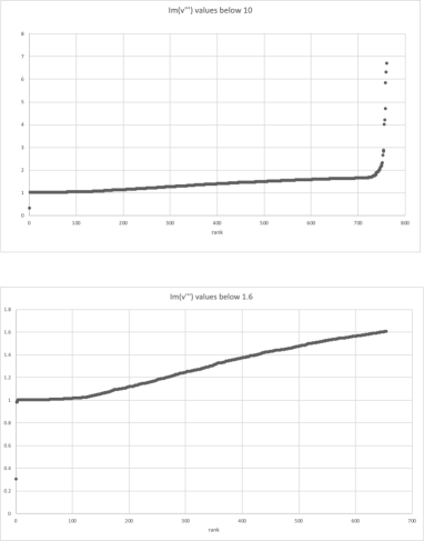
Figure 5: $\Im(v^{\prime\prime\prime})$ values versus their ranks.

$\mathscr{O}\cong\hat{\mathbb{C}}$ case

For the species data set (Table 1), consider that a sequential operation is an exact form. As in [Adachi, 2017], setting operation III as $\Re(v)=v$, $\Im(v)=\mu_{l}=e^{(\Re(v)/b)E(N)}$, $\Re(v^{\prime})=E[l]=l=\ln(N_{k})/\ln(\Im(v))$, $\Im(v^{\prime})=e^{(\Re(v^{\prime})/b)E(N)}$, $\Re(v^{\prime\prime})=\ln(N_{k})/\ln(\Im(v^{\prime}))$, $\Im(v^{\prime\prime})=e^{(\Re(v^{\prime\prime})/b)E(N)}$, $v^{\prime\prime\prime}$ by $\Re(v^{\prime\prime\prime})=\ln(N_{k})/\ln(\Im(v^{\prime\prime}))$, and $\Im(v^{\prime\prime\prime})=e^{(\Re(v^{\prime\prime\prime})/b)E(N)}$, we have $\Re(v)\simeq\Re(v^{\prime\prime})\simeq 0$, $\Im(v)\simeq\Im(v^{\prime\prime})\simeq 0$, $\Re(v^{\prime})\simeq\Re(v^{\prime\prime\prime})\simeq 0$, $\Im(v^{\prime})\simeq\Im(v^{\prime\prime\prime})\simeq 0$, suggesting that an actual/potential of species creates an actual/potential appearance of the adapted hierarchy above two layers. Recall that this is a short exact sequence; the morphism $\Im$ becomes monomorphism and $\Re(ln)$ becomes epimorphism. Furthermore, $\mathrm{Im}\Im$ is equal to $\mathrm{Ker}\Re(ln)$. Obviously there also exists a homomorphism $h:\Im(v^{\prime})\rightarrow\Re(v^{\prime})$, $h:\Re(v^{\prime\prime})\rightarrow\Im(v^{\prime})$, $h:\Im(v^{\prime\prime})\rightarrow\Re(v^{\prime\prime})$ or $h:\Re(v^{\prime\prime\prime})\rightarrow\Im(v^{\prime\prime})$, and the short exact sequence is a split. These are abelian groups and $\Re(v^{\prime})\simeq\Im(v)\oplus\Im(v^{\prime})$, $\Im(v^{\prime})\simeq\Re(v^{\prime})\oplus\Re(v^{\prime\prime})$, $\Re(v^{\prime\prime})\simeq\Im(v^{\prime})\oplus\Im(v^{\prime\prime})$, $\Im(v^{\prime\prime})\simeq\Re(v^{\prime\prime})\oplus\Re(v^{\prime\prime\prime})$. The data show that an actual layer is a direct sum of a potential layer below and a potential layer. The data also show that a potential of the layer is a direct sum of a real layer and a layer above the layer. Finally, defining a Galois action $\mathrm{Gal}(L/K)$, actions defined by $\Re(v^{\prime})/\Im(v)\simeq\Im(v^{\prime})$, $\Im(v^{\prime})/\Re(v^{\prime})\simeq\Re(v^{\prime\prime})$, $\Re(v^{\prime\prime})/\Im(v^{\prime})\simeq\Im(v^{\prime\prime})$, and $\Im(v^{\prime\prime})/\Re(v^{\prime\prime})\simeq\Re(v^{\prime\prime\prime})$ are all Galois, achieving our goal for defining proper Galois actions with a topology of $v$ for biological hierarchies. A species is thus likely to emerge from the interaction of species.

For species, consider that a sequential operation in the previous sections is an exact form. As in [Adachi, 2017], setting an operation III, we have $\Re(v)\simeq\Re(v^{\prime\prime})\simeq 0$ and $\Im(v)\simeq\Im(v^{\prime\prime})\simeq 0$, but no further (Table 1), suggesting that an actual/potential of species creates an actual/potential appearance of the adapted hierarchy above two layers, which diminishes in the three layers above. This might reflect effects from different time scales among different layers [Adachi, 2015]. Similar to the previous section, $\Re(v^{\prime})\simeq\Im(v)\oplus\Im(v^{\prime})$ and $\Im(v^{\prime})\simeq\Re(v^{\prime})\oplus\Re(v^{\prime\prime})$.

From the III morphisms, we can draw a short exact sequence corresponding to $\Re(v)\to\Im(v)\to l=\Re(v^{\prime})\to l\times(\Im(s)=\Im(v^{\prime}))\to\Re(v)=\Re(v^{\prime\prime})$,

$$0\to\mathcal{A}(u)\overset{\iota}{\to}\mathcal{B}(u)\overset{\mathrm{sp}}{\to}\mathcal{C}(u\times\sqrt{-1}S^{*})\to 0,$$ (132)

regarding $g=l$ as a specific spectrum of the Schwartz distribution (or Sato hyperfunction [Sato, 1959] [Sato, 1960]) of a microfunction $\mathrm{sp}\ g$ [Sato, 1969] [Morimoto, 1970]. Not only addition, but also multiplication is feasible for $-s$ in this regard.

Congruent zeta function

Hereafter we will adhere to the situation where $\mathscr{O}\cong\hat{\mathbb{C}}$. For the other aspect, instead of $\Im(v^{\prime})$, we can consider $\mathbb{Z}/l\mathbb{Z}$, by $1/l$-powered $\Im(v^{\prime})$, state a $p$-adic number correspondence, and then take a valuation of it. Universal coefficient theorems [Bott and Tu, 1982],

$$\begin{split}0\to\mathrm{Ext}(H_{q-1}(X,A),G)\to H^{q}(X,A;G)\\ \to\mathrm{Hom}(H_{q}(X,A),G)\to 0,\end{split}$$ (133)

could be described as

$$0\to\mu_{l}\to E[l]\to\mathbb{Z}/l\mathbb{Z}\to 0,$$ (134)

making an exact sequence, with $\Re(s)$ value in the middle level between populational $\Re(v)$ value and its fractal $\Re(v^{\prime\prime})$ value. $E[l]\to\mathbb{Z}/l\mathbb{Z}$ is an injection and $\mathbb{Z}/l\mathbb{Z}\to 0$ an epimorphism. The image of the former is the kernel of the latter. Homology backwards is a homomorphism of the cohomology, and the exact sequence splits. These are abelian groups and $E[l]\cong\mathbf{\mu}_{l}\oplus\mathbb{Z}/l\mathbb{Z};\mathbb{Z}/l\mathbb{Z}\cong E[l]\oplus 0$. A real level is constituted by a direct sum of a potential level below and its own potential. A potential level is constituted by a direct sum of a real level below and a real level above. $E[l]/\mathbf{\mu}_{l}\cong\mathbb{Z}/l\mathbb{Z};\mathbb{Z}/l\mathbb{Z}/E[l]\cong 0$ are Galois actions and a representation of an étale topology $\ell$ is obtained, concomitantly with information of interactions among different levels of hierarchies. Species should appear two layers above the population layer. [Adachi, 2015] reports results where the point mutation rate is on the order of $10^{-8}$ and speciation is on the order of $10^{-25}$, roughly above a square of $10^{-8}$ over $10^{-8}$. This calculation could be modeled by a simple critical phenomenon of dendrogram percolation. In this model, approaching $1/2-0$ probability of mutation maintenance leads to divergence in cluster size. Regarding non-trivial $\zeta(s)=0$ as a seed for speciation, a $\sim 10^{8}$ population is on the same order as a branch for being identical to ancestors or different from them at each genome base pair. A dendrogram can be regarded as a phylogenetic tree for dividing cells, which is common to both asexually propagating organisms and a constituent of sexually reproducing organisms at the level of cell division of germ line cells, strictly correlated to mutation during cell cycle processes. These facts exhibit $\ell$ and Galois actions can adequately describe interhierarchical interactions.

The logic above would suggest application of Grothendieck groups. Let the situation be a Noetherian ring, i.e., $B$ is the ring. Let $F(B)$ be the set of all isomorphisms of $B$-modules. Let $C_{B}$ be the free abelian group generated by $F(B)$. The short exact sequence above is associated with $(\mu_{l})-(E[l])+(\mathbb{Z}/l\mathbb{Z})$ of $C_{B}$ (() is an isomorphism). Let $D_{B}$ be the subgroup of $C_{B}$. The quotient group $C_{B}/D_{B}$ is a Grothendieck group of $B$ related to potential of $s,w$ layers, denoted by $K(B)$. If $E[l]$ is a finitely generated $B$-module, $\gamma(E[l])$ would be the image of $(E[l])$ in $K(B)$. There exists a unique homomorphism $\lambda_{0}:K(B)\to G$ such that $\lambda(E[l])=\lambda_{0}(\gamma(E[l]))$ for all $E[l]$ when $G$ is an abelian group of the $B$-module. This representation corresponds to the Stone-von Neumann theorem in this restricted situation. $B$ is generated by $\gamma(B/p)$ when $p$ corresponds to species in a biological sense. If $B$ is a principal ideal domain constituting a single niche without cooperation of distinguished niches, $K(B)\cong\mathbb{Z}$, and this is suitable when considering biological numbers for individuals. Considering different $E[l]$, $M_{l}$, and $N_{l}$, and the set of all isomorphisms of a flat $B$-module $F_{1}(B)$, $\gamma_{1}(M_{l})\cdot\gamma_{1}(N_{l})=\gamma_{1}(M_{l}\otimes N_{l});\gamma_{1}(M_{l})\cdot\gamma(N_{l})=\gamma(M_{l}\otimes N_{l});K_{1}(A)\cong\mathbb{Z}$ with tensor products. Furthermore, if $B$ is regular, $K_{1}(B)\to K(B)$ is an isomorphism. The sum of interactions for different niches (not interacting between distinguished niches) is thus calculable as integers by a Grothendieck group. If the calculation does not lead to integers, the situation involves interactions among distinguished niches. Algebraic expansion of this ring thus introduces entirely different niches to the original ring. If $a\in K,f(x)=x^{l}-x-a,\alpha\in\bar{K},f(\alpha)=0,\alpha\notin K(\alpha\in\partial K)$, $f(x)$ is irreducible on $K$, $L=K(\alpha)$ is a Galois extension, and $\mathrm{Gal}(L/K)\cong\mathbb{Z}/l\mathbb{Z}$. $\alpha$ is from the hierarchy above based on a new ideal.

To unify the sections introducing Galois $H^{i}$ and the preceding sections regarding the time arrow, consider $X,Y$, which are eigen and smooth connected algebraic curves on an algebraic closed field.

$$\begin{split}H^{i}(X_{\bar{k}},\mathbb{Q}_{\ell})\xrightarrow{\mathrm{pr}_{1}^{*}}H^{i}(X_{\bar{k}}\times_{\bar{k}}Y_{\bar{k}},\mathbb{Q}_{\ell})\\ \xrightarrow{\cup\mathrm{cl}(\gamma)}H^{i+2d}(X_{\bar{k}}\times_{\bar{k}}Y_{\bar{k}},\mathbb{Q}_{\ell}(d))\xrightarrow{\mathrm{pr}_{2_{*}}}H^{i}(Y_{\bar{k}},\mathbb{Q}_{\ell}),\end{split}$$ (135)

when $\gamma$ is an algebraic correspondence from $Y$ to $X$. If we assume $X$ and $Y$ correspond to different time points, the above diagram,

$$\gamma^{*}:H^{i}(X_{\bar{k}},\mathbb{Q}_{\ell})\rightarrow H^{i}(Y_{\bar{k}},\mathbb{Q}_{\ell})$$ (136)

describes the time development of the system. To dissect the contributions of each component on the time developing system, let $\kappa_{m}$ be an $m$-dimensional expansion of $\kappa$, which is a finite field of a residue field of an integer ring $O_{K}$ on $K$. When the eigen smooth scheme $Y$ is on $\kappa$,

$$\sum_{i=0}^{2d}(-1)^{i}\mathrm{Tr}(\mathrm{Frob}_{v}^{m};H^{i}(Y_{\bar{k}},\mathbb{Q}_{\ell}))=\sharp Y(\kappa_{m})$$ (137)

[Deligne, 1977] [Rapoport and Zink, 1982].

When $Y$ is finite, a congruent zeta function is

$$Z(Y,T)=\exp(\sum_{n=1}^{\infty}\frac{\sharp Y(\kappa_{n})}{n}T^{n}).$$ (138)

Setting

$$P_{i}(Y,T)=\det(1-\mathrm{Frob}_{v}T;H^{i}(Y_{\bar{k}},\mathbb{Q}_{\ell}))$$ (139)

results in

$$Z(Y,T)=\prod_{i=0}^{2\dim Y}P_{i}(Y,T)^{(-1)^{i+1}}.$$ (140)

To separate each contribution of $H^{i}$, consider Weil conjectures [Deligne, 1974] [Deligne, 1980.], and $P_{i}(Y,T)$ and $P_{j}(Y,T)$ are disjoint when $i\neq j$. $P_{i}(Y,T)$ and $\mathrm{Tr}(\mathrm{Frob}_{v}^{m};H^{i}(Y_{\bar{k}},\mathbb{Q}_{\ell}))$ are thus calculable and this deciphers each contribution of $P_{i}(Y,T)$s. Examples of the calculation are provided in Tables 5 & 6. Generally, large positive zeta values represent highly adapted situations, whereas large negative zeta values represent highly disadapted situations and zero values are neutral situations. $P_{0},P_{1},P_{2}$ correspond to $\Re(v^{\prime}),\Im(v^{\prime}),\Re(v^{\prime\prime})$. For $\Re(v^{\prime}),\Re(v^{\prime\prime})$, values close to zero represent large contributions, and for $\Im(v^{\prime})$, large values represent large contributions. The inverses of $\Re(v^{\prime}),\Re(v^{\prime\prime})$ scale for $\Im(v^{\prime})$. The important point here is that by utilizing a congruent zeta function, we can visualize a contribution from each hierarchy.

Table 5: Calculations for Washidu East quadrat

$Z$ (congruent)	P. pallidum	D. purpureum	P. violaceum
April	-	-	-
June	0.009378	151.1	9.272
July	-	-	-
August	-	-	-
September	114.7	30.89	-
October	334.6	-540.4	-
November	0.02561	-	-54.13
December	-	-	-
January	-	-	-

$P_{0}$	P. pallidum	D. purpureum	P. violaceum
April	-	-	-
June	-1.288	-0.06806	-0.1520
July	-	-	-
August	-	-	-
September	-1.163	-0.7248	-
October	-0.8250	0.02954	-
November	-1.002	-	0.1790
December	-	-	-
January	-	-	-

(continues.)

$P_{1}$	P. pallidum	D. purpureum	P. violaceum
April	-	-	-
June	0.7635	-10.29	-1.253
July	-	-	-
August	-	-	-
September	-133.4	-22.39	-
October	-276.1	-15.96	-
November	0.7480	-	-9.689
December	-	-	-
January	-	-	-

$P_{2}$	P. pallidum	D. purpureum	P. violaceum
April	-	-	-
June	-63.23	1.000	0.8886
July	-	-	-
August	-	-	-
September	1.000	1.000	-
October	1.000	0.9999	-
November	-29.13	-	1.000
December	-	-	-
January	-	-	-

Table 6: Calculations for Washidu West quadrat.

$Z$ (congruent)	P. pallidum	D. purpureum	P. violaceum
April	-	-	-
June	-	-	-
July	8.135	0.002196	97.00
August	123.7	29.31	-
September	26.54	-106.1	0.0001892
October	99.51	-	26.36
November	-	-	-
December	-	-	-
January	-	-	-

$P_{0}$	P. pallidum	D. purpureum	P. violaceum
April	-	-	-
June	-	-	-
July	-0.1936	-2.208	-0.1174
August	-1.306	-0.9804	-
September	-0.6856	0.08601	-8.157
October	-1.141	-	-0.7729
November	-	-	-
December	-	-	-
January	-	-	-

(continues.)

$P_{1}$	P. pallidum	D. purpureum	P. violaceum
April	-	-	-
June	-	-	-
July	-1.483	0.9810	-11.39
August	-161.6	-28.74	-
September	-18.19	-9.126	1.000
October	-113.6	-	-20.37
November	-	-	-
December	-	-	-
January	-	-	-

$P_{2}$	P. pallidum	D. purpureum	P. violaceum
April	-	-	-
June	-	-	-
July	0.9417	-202.2	1.000
August	1.000	1.000	-
September	1.000	1.000	-647.9
October	1.000	-	1.000
November	-	-	-
December	-	-	-
January	-	-	-

From these theorems, we can deduce that $\mathbf{P}^{2}$ is a pencil on elliptic curves with a section of order two and an additional multisection. Setting $\zeta=e^{2\pi i/3}=(e^{\pi i/3})^{2}$ on the initial condition of $\mathbf{P}^{2}$ at the point $x_{a}=0$,

$$t=\zeta+1,X(\zeta+1)=\frac{1}{1-\zeta},X^{\prime}(t)=\frac{1}{3}.$$ (141)

In the PzDom model, $1/\Im(s-1)\approx e^{\pi i/3}$ for predicting the future and $t$ is an addition of $1$ to interactive $(e^{\pi i/3})^{2}$ if $\Re(s-1)$ is neglectable. When in close proximity to trivial zero points of Riemann $\zeta$, $t\sim 1$ and $X(t)\sim 1$. $X^{\prime}(t)=\frac{1}{3}$ thus represents a ($2+1$)-dimensional system.

System dimensions are thus reduced to 2+1. For reproducing the kernels, let $q$ be in $(Q^{\infty})^{\Gamma}(\mathbf{H}^{*})$. Then,

$$q(w)dw^{2}=\frac{12}{\pi}(\int_{\mathbf{H}}\frac{q(\bar{z})\Im(z)^{2}}{(z-w)^{4}}|dz|^{2})dw^{2},$$ (142)

where $w=\alpha/\beta$ and $z:=(\alpha\zeta+\bar{\alpha})/((\beta\zeta+\bar{\beta})$. The term in parentheses is the reproduced kernel (Prop. 5.4.9 of [Hubbard, 2006]).

Now consider $q$ difference $\mathrm{Painlev\acute{e}}$ VI with $\hat{\mathfrak{gl}}_{3}$ hierarchy. $q$ could be equal to $-s$, and $y(x+1)=\frac{1-q^{x}}{1-q}y(x)=(\sum_{i=0}^{x-1}q^{i})y(x)$ can be converted from $q$ to $-s$, when $x\to\infty$.

Setting $|q|>1$, $t$ as an independent variable, and $f$, $g$ as dependent variables,

$$\begin{split}T(g)=\frac{(f-ta_{1})(f-ta_{2})b_{3}b_{4}}{g(f-a_{3})(f-a_{4})},T^{-1}(f)\\ =\frac{(g-tb_{1})(g-tb_{2})a_{3}a_{4}}{f(g-b_{3})(g-b_{4})},\end{split}$$ (143)

where

$$f=-\frac{\mathcal{A}_{0}^{12}}{\mathcal{A}_{1}^{12}},g=\frac{(\mathcal{A}_{0}^{12}+x_{1}\mathcal{A}_{1}^{12})(\mathcal{A}_{0}^{12}+x_{1}q^{\alpha_{1}+1}\mathcal{A}_{1}^{12})}{q(\mathcal{A}_{0}^{11}(\mathcal{A}_{1}^{12})^{2}-\mathcal{A}_{1}^{11}\mathcal{A}_{0}^{12}\mathcal{A}_{1}^{12}+q^{\beta_{2}+1}(\mathcal{A}_{0}^{12})^{2})}.$$ (144)

$$\mathcal{A}_{0}^{12}=q^{\alpha_{1}+\alpha_{2}+2}x_{1}x_{2}\omega_{13}\bar{w}_{32},$$ (145)

$$\mathcal{A}_{1}^{12}=q^{\alpha_{1}+1}x_{1}\omega_{11}\bar{w}_{12}+q^{\alpha_{2}+1}x_{2}\omega_{12}\bar{w}_{22},$$ (146)

$$\mathcal{A}_{0}^{11}=q^{\alpha_{1}+\alpha_{2}+2}x_{1}x_{2}(1+\omega_{13}\bar{w}_{31}),$$ (147)

$$\begin{split}\mathcal{A}_{1}^{11}=-q^{\alpha_{1}+1}x_{1}(1+\omega_{12}\bar{w}_{21}+\omega_{13}\bar{w}_{31})\\ -q^{\alpha_{2}+1}x_{2}(1+\omega_{11}\bar{w}_{11}+\omega_{13}\bar{w}_{31})\end{split}$$ (148)

and considering $q=-b\ln D$ of the PzDom model, local time development can be easily calculated. $(a_{1},a_{2},a_{3},a_{4})$; $(b_{1},b_{2},b_{3},b_{4})$ have 4 parameters interacting with each other in this soliton equation of similarity reduction [Jimbo, 1996] [Kakei and Kikuchi, 2007]. In other words, we are treating a direct sum of two Virasoro algebras, or a Majorana fermion analog and a super-Virasoro algebra [Bershtein and Shchechkin, 2015].

Further considerations of 1+1 dynamics

There is another way of considering system dynamics with $q$, starting from a Young tableau. Let $S$ be a finite or countable set, for example, as the measures of species density as $\mathrm{Spec}\mathbb{Z}$. For $\Re(s)\leq 1/2$, let an absolute value of an absolute zeta function $\zeta_{K}=\zeta_{\mathbb{G}_{m}/F_{1}}(x,y)=|\frac{s(x,y)}{(s-1)(o,y)}|;x,y\in S$ where $\mathbb{G}_{m}=GL(1)$. For $\Re(s)>1/2$, and let an absolute value of an inverse of an absolute zeta function $\zeta_{K}=\frac{1}{\zeta_{\mathbb{G}_{m}/F_{1}}(x,y)}=|\frac{(s-1)(o,y)}{s(x,y)}|;x,y\in S$. $\zeta_{K}$ becomes a Martin kernel. Let a distance function $D_{\delta}(x,y)=\sum_{z\in S}C_{z}(|\zeta_{K}(z,x)-\zeta_{K}(z,y)|+|\delta_{zx}-\delta_{zy}|)$, where $\delta$ is the delta function. For a distance space $(S,D_{\delta})$, a topology of $S$ determined by $D_{\delta}$ is a discrete topology and $(S,D_{\delta})$ is totally bounded. A completion of $(S,D_{\delta})$ will be set as $\hat{S}$. Let a Martin boundary $\partial S=\hat{S}\backslash S$ be a ($d-1$)-dimensional species density not restricted to a random walk or transition probability. $S^{d}$ represents all possibilities of $S^{d-1}$ with a time dimension. Furthermore, a set of $S^{d-1}$ can be expressed by a Young tableau in a Frobenius coordinate system. Taking a Maya diagram of the tableau distributes the data to a single dimension. Therefore, the 3-dimensional system is in fact represented as a 1-dimensional system, a set of $F_{1}=F_{q}$. In this context, a set of the individual numbers of species is over $\mathbb{Z}$ and a time $X$ is a flat algebra $\Lambda$-space over $\mathbb{Z}$. A $\Lambda$-structure on $X$ is $\psi_{p}:X\to X$, where $\psi$ is $X\times_{\mathrm{Spec}\mathbb{Z}}\mathrm{Spec}\mathbb{F}_{p_{c}}$. In other words, $\Lambda=\mathbb{Z}[\mathrm{Gal}(\mathbb{Z}/\mathbb{F}_{p_{c}})]$. $p_{c}=1$ when there is no hierarchy/period in our analysis and, for example, $p_{c}=2$ in protein or species data sets described above. Therefore, the hierarchy extends from $F_{1}$ to $F_{2}$. $M_{n/\mathbb{F}_{1}}=\underline{\mathrm{Hom}}_{\mathbb{G}_{m}/F_{1}}(\mathbb{A}^{n},\mathbb{A}^{n})=\zeta_{K};GL_{n/\mathbb{F}_{1}}=\underline{\mathrm{Aut}}_{\mathbb{G}_{m}/F_{1}}(\mathbb{A}^{n})=S^{n}$ and thus $s\in\mathbb{G}_{m}$ and $s-1\in F_{1}$ when $\Re(s)\leq 1/2$ and $s-1\in\mathbb{G}_{m}$ and $s\in F_{1}$ when $\Re(s)>1/2$. $q\in\mathbb{G}_{m}$ and $\mathrm{Spec}(q)$ is $\mathrm{Spec}(s)$ or $\mathrm{Spec}(s-1)$. Since $D=e^{s/b}$ is calculable in with a root of time $t$, temperature $b_{t}$ at time point $t^{2}$ and temperature $b_{t-1}$ at time point $(t-1)^{2}$ when time is properly scaled, the dynamics of $q$ can be calculated by this basal information. See [Borger, 2009] for further details in this respect as relates to Grothendieck’s Riemann Roch theorem. This is another explanation as to why a 1-dimensional system with a certain topology leads to $3+1$ dynamics.

$\wp$ as evaluations for interactions

Take Wallis’ formula:

$$\lim_{n\to\infty}\frac{1}{\sqrt{n}}\cdot\frac{2\cdot 4\cdot\bullet\bullet\bullet\cdot(2n)}{1\cdot 3\cdot\bullet\bullet\bullet\cdot(2n-1)}=\sqrt{\pi}.$$ (149)

The upper product of even numbers could be a product of bosonic multiplications, and the lower product of odd numbers could be that of fermionic multiplications. The square of them divided by $n$ as an average number of actions would result in $\pi$. $\pi$ is thus the number ratio of boson multiplications and fermion multiplications. In other words, an area of a circle corresponds to boson actions and the square of the radius corresponds to fermion actions. Globally there are $\sim 3$ times more bosonic actions than fermionic actions. For further expansion for the bosonic even $-s$ (without $s=0$) with $\mu(n)=1$, Weierstraß $\wp(1/n)=\sum_{s=-2}^{negative\ even\neq 0}(1/n)^{s}$ and a $((s/2+1)\times n)(n\times 1)$ matrix would calculate a set of patch quality $P_{s}$ of bosons involving a future status of $s=-2$. Similarly, even $-w$ with $\mu(n)=-1$, $-\wp(1/n)=-\sum_{w=-2}^{negative\ even\neq 0}(1/n)^{w}$, and a $((w/2+1)\times n)(n\times 1)$ matrix would calculate a set of patch quality $-P_{w}$ of fermions involving a future status of $w=-2$. Regarding $w=s-1$, $P(s)=P_{s}-P_{w=s-1}=\zeta(s)+n+n^{2}$ and the Riemann $\zeta$ function can be related to patch quality. Population bursts with these even $s$ (odd $w$) could be calculated by $P_{s}\to+\infty$ with negative even $s$ (negative odd $w$), or in lower extent of bursting, $P_{w}\to\mp\infty$ with $s\to 1\mp 0(w\to 2\mp 0)$. Since $P(0)\neq 0$ and $P(0)\to+\infty$, considering $P(s)=\wp(1/n)+\wp(1/n)/n$ and $a_{k},b_{k}$ as zero points and poles of the function,

$$\begin{split}f_{P}(1/n)=C_{P}\prod_{k=1}^{\infty}\frac{\wp(1/n)-\wp(a_{k})}{\wp(1/n)-\wp(b_{k})}\\ \times\prod_{k=1}^{\infty}\frac{\wp(1/n)/n-\wp(a_{k})/n}{\wp(1/n)/n-\wp(b_{k})/n}=0\end{split}$$ (150)

because the constant $C_{P}=0$ when $s=0$ [Ahlfors, 1979]. Thus $s=0(w=-1)$ means every singularity can be considered as a zero ideal adopting $f_{P}$. We can regard a logarithm of $s$ as a fitness when the fitness is sufficiently small. If we regard Weierstraß $\zeta(z;\Lambda)=\frac{1}{z}+\sum_{w\in\Lambda^{*}}(\frac{1}{z-w}+\frac{1}{w}+\frac{z}{w^{2}})$ (not Riemann zeta) as a distribution function, an additive operation for fractal dimensions $s_{1},s_{2}$ results in

$$\zeta(s_{1}+s_{2})=\zeta(s_{1})+\zeta(s_{2})+\frac{1}{2}\frac{\wp^{\prime}(s_{1})-\wp^{\prime}(s_{2})}{\wp(s_{1})-\wp(s_{2})}.$$ (151)

This means the third term on the right is a contribution of different fractal hierarchies, besides a direct sum of distribution functions. Tables 7 to 11 present values for the Weierstraß zeta function, Weierstraß $\wp$, $\wp^{\prime}$, and interaction terms. Note that at Washidu West in September, Pv-Dp-Pp interacted strongly in that order. In October, there is also a strong interaction of Pv-Pp. Compared with Washidu West, Washidu East exhibited weaker interaction and was dominated by Pp. It is also notable that the strengthes of hetero-interactions were generally weaker than those of homo-interaction, as supposed. Of course, utilizing population data instead of species data elucidates similar or larger values for hetero-interaction terms compared with homo-interaction terms (data not shown), as was expected.

Table 7: Weierstraß $\zeta$ values.

Weierstraß $\zeta$	WE P. pallidum	WE D. purpureum	WE P. violaceum
April
June	2.290e15 - 5.081e15i	5.648e51 + 1.513e52i	3.036e32 + 1.2783e32i
July
August
September	-9.284e28 - 2.716e28i	-1.501e23 + 3.448e23i
October	-3.307e36 - 2.666e37i	-1.220e35 - 2.047e35i
November	3.579e14 - 1.003e15i		2.065e59 + 9.395e59i
December
January

(continues.)

Weierstraß $\zeta$	WW P. pallidum	WW D. purpureum	WW P. violaceum
April
June
July	2.329e35 + 1.735e35i	7.052e8 - 2.352e10i	4.950e53 + 1.630e54i
August	-4.121e28 - 1.547e28i	-1.075e22 + 3.286e22i
September	1.493e39 + 1.008e39i	6.076e48 + 1.023e49i	1.220 + 0.02924i
October	-4.379e28 - 1.562e28i		-1.440e22 + 4.328e22i
November
December
January

Table 8: $\wp$ values.

$\wp$	WE P. pallidum	WE D. purpureum	WE P. violaceum
April
June	1.709e16 + 9.720e15i	-2.966e51 + 1.066e51i	-1.304e32 + 2.778e32i
July
August
September	5.052e28 - 1.081e29i	-5.829e23 - 4.100e23i
October	1.694e37 - 1.838e35i	1.622e35 - 7.066e34i
November	3.600e15 + 1.691e15i		-9.903e58 + 2.100e58i
December
January

(continues.)

$\wp$	WW P. pallidum	WW D. purpureum	WW P. violaceum
April
June
July	-1.334e35 + 1.676e35i	1.259e11 + 1.727e10i	-2.717e53 + 7.949e52i
August	2.719e28 - 4.871e28i	-6.167e22 - 3.546e22i
September	-5.774e38 + 7.958e38i	-1.837e38 + 7.905e37i	-0.8200 + 4.042i
October	6.491e22 - 1.137e22i		3.434e17 - 1.790e18i
November
December
January

Table 9: $\wp^{\prime}$ values I.

$\wp^{\prime}$	WE P. pallidum	WE D. purpureum	WE P. violaceum
April
June	3.841e16 - 5.488e16i	1.938e50 + 5.613e50i	2.450e32 + 1.2734e32i
July
August
September	-1.181e29 - 7.904e28i	-9.494e23 + 8.939e23i
October	1.048e36 - 1.027i	-3.553e34 - 1.217e35i
November	7.322e15 - 1.234e16i		2.058e57 + 1.008e58i
December
January

Table 10: $\wp^{\prime}$ values II.

$\wp^{\prime}$	WW P. pallidum	WW D. purpureum	WW P. violaceum
April
June
July	1.162e35 + 9.874e34i	1.594e11 - 6.432e11i	1.231e52 + 4.372e52i
August	-5.395e28 - 4.181e28i	-9.400e22 + 1.055e23i
September	4.088e38 + 3.182e38i	3.442e47 + 6.318e47i	14.97 - 8.365i
October	-5.744e28 - 4.312e28i		-1.223e23 + 1.360e23i
November
December
January

Table 11: Hetero-interaction terms.

hetero-interaction	WE		WW
Pp-Dp (June)	0.001160 - 0.09419i	Pp-Dp (Jul)	0.01142 - 0.3558i
Pp-Pv (June)	0.01818 - 0.4494i	Pp-Pv (Jul)	0.0008154 - 0.08021i
Dp-Pv (June)	0.001160 - 0.09419i	Dp-Pv (Jul)	0.0008154 - 0.08021i
September	0.09055 - 0.5885i	August	0.09149 - 0.6049i
October	0.03433 - 0.3021i	Pp-Dp (Sep)	-2.372e8 + 3.704e8i
November	0.0003791 - 0.05081i	Pp-Pv (Sep)	0.008871 - 0.2633i
		Dp-Pv (Sep)	-1.659e8 - 1.791e9i
		October	-3.728e5 - 3.975e5i

For further clarification, regarding $\wp$ as an elliptic function,

$$\wp^{\prime 2}=4\wp^{3}-g_{2}\wp-g_{3}$$ (152)

is a normal form without multiple root. Rationals exist, $F(\wp(u)),G(\wp(u))$ as Legendre canonical forms of elliptic integrals, such that any elliptic function $f(u)=F(\wp)+G(\wp)\wp^{\prime}$. Thus a particular state during time procedure $\wp^{\prime}$ can be related to any elliptic function form by a particular pair of Legendre canonical forms. Utilizing Weierstraß $\wp$ is thus closely related to abstraction of interaction of the states, with a cube of $\wp$ itself. Setting $\Omega$ as a period of $f(u)$, the canonical form $K(\Omega)\cong\mathbb{C}[x,y]/(y^{2}-4x^{3}+g_{2}x+g_{3})$, where $\mathbb{C}[x,y]$ is an integral domain. The ideal thus characterizes the observation phenomena related to $F,G$.

To develop the evaluation, $s$ can be regarded as the elliptic function $f(u)$ via $p,l$ double periodicity, and a linear plot of $f(u)$ against $\wp^{\prime}$ shows $F,G$ values. Basically, due to empirically massive values for $\wp^{\prime}$, $G\sim 0$ and $F$ are almost identical to either of the $s$ values selected for calculating the interaction. By this method, one can evaluate which of the interacting partners plays a major role in the interaction. The results are shown in Table 12; in WE, the climax species Pp dominated, while in WW, pioneering species Dp and Pv had significant roles [Adachi, 2015]. Note that $F,G$ are solutions for corresponding hypergeometric differential equations. Thus $g_{2},g_{3}$ become apparent during the time development process. $\omega$ can be calculated by $g_{2}=60\sum_{\omega\in\Lambda^{\prime}}\frac{1}{\omega^{4}},g_{3}=140\sum_{\omega\in\Lambda^{\prime}}\frac{1}{\omega^{6}}$. Riemann’s theta relations showed how a ($3+1$)-dimensional system could be rearranged to a $2+2$ system. Tables 13 & 14 show calculated values for $g_{2},g_{3}$ in normal form of the elliptic curves.

Table 12: $F$ values and contributions.

$F$	WE	major		WW	major
Pp-Dp (June)	0.7693+8.182i	Pp	Pp-Dp (Jul)	0.5752+5.331i	Dp
Pp-Pv (June)	0.7693+8.182i	Pp	Pp-Pv (Jul)	1.262+39.31i	Pp
Dp-Pv (June)	1.258+31.10i	Pv	Dp-Pv (Jul)	0.5752+5.331i	Dp
September	3.078+14.99i	Pp	August	2.879+13.80i	Dp
October	4.907+38.67i	Dp	Pp-Dp (Sep)	1.790+53.12i	Pp
November	0.7481+7.726i	Pp	Pp-Pv (Sep)	0.3186+2.028i	Pv
			Dp-Pv (Sep)	0.3186+2.028i	Pv
			October	2.905+13.93i	Pv

Table 13: $g_{2},g_{3}$ values I.

Normal form	$g_{2}$	$g_{3}$	int.	const.	synch.
Pp-Dp (June)	3.066e103-2.529e103i	-7.698e119+1.343e119i	-	+	anti
Pp-Pv (June)	-2.408e65-2.899e65i	1.298e81+7.295e81i	+	-	anti
Dp-Pv (June)	3.066e103-2.529e103	-3.028e135-1.182e136i	-	+
September	-3.651e58-4.368e58i	-3.373e81-4.044e82i	+	+	for
October	1.159e75-2.991e73i	-1.859e110+8.674e109i	-	+	anti
November	3.747e118-1.663e118i	-1.630e134-3.473e132i	-	+

Table 14: $g_{2},g_{3}$ values II.

Normal form	$g_{2}$	$g_{3}$	int.	const.	synch.
Pp-Dp (Jul)	-4.118e70-1.788e71i	2.322e82+2.096e81i	+	-	anti
Pp-Pv (Jul)	-1.728e107+2.700e107i	-6.829e142+7.054e141i	+	+	for
Dp-Pv (Jul)	1.691e198-1.728e107i	-3.697e118+1.709e118i	-	+	anti
August	-1.060e58-6.532e57i	-2.706e79-8.852e80i	+	+	for
Pp-Dp (Sep)	-9.168e77-4.559e78i	-5.398e116-7.349e116i	+	+	for
Pp-Pv (Sep)	-1.199e78-3.676e78i	-1.584e79+1.834e78i	+	+
Dp-Pv (Sep)	1.099e77-1.162e77i	-3.794e77-5.397e77i	-	+
October	1.634e46-5.905e45i	4.963e63+3.128e64i	-	-

2.15 Renormalization and fractals among sets beyond (empty) boundaries

In physics, renormalization is widely applied to accommodate the divergence of terms (e.g., [Benfatto and Gallavotti, 1995], [Cardy, 1996]) despite its fragility in rigorous mathematics. Importantly, renormalization could be intrinsically related to the development of fractals, which apparently disappear from the layer of interest, while at a larger scale higher-order fractals are manifested. Herein, we commence by deciphering a model of magnetization in a scaling hypothesis by focusing on the fact that the parameters involved are exactly equivalent to the imaginary parts of particular nontrivial zero points of a Riemann zeta function. Utilizing an analogy of magnetization to species dynamics in biology, we posit that fractals can explain many salient aspects. To approach this problem, we introduce two mathematical ideas - étale and Frobenioid.

Broadly speaking, an étale is a category-theoretic abstraction of the notion of a category if it has a lifting property that is analogous to being a local diffeomorphism, i.e., intuitively a function between smooth manifolds that preserves the local differentiable structure. A Frobenioid is a category-theoretic abstraction of the notion of a category of line bundles or monoids of divisors over a base category of topological localizations such as a Galois [Mochizuki, 2020a]. A Gaussian monoid would roughly correspond to a harmonic function related to an étale or Frobenioid. Thus, $p$ (persistent homology) or $l$ (étale cohomology) can be evaluated as the number of Gaussian monoids. For Cartesian coordinates (implying entanglement of each line as in [Witten, 2017]), the system according to étale and Frobenioid is described as de Rham side or Hodge filtration, designated as the Frobenius picture in [Mochizuki, 2020b]. For polar coordinates, it is described as the étale side or Galois action on torsion points, designated as the étale picture in [Mochizuki, 2020b]. The Frobenius picture corresponds to the last figure we propose here. For the étale picture, a gradient is étale acting on self-organization, whilst a rotation acting on circulation is Frobenioid, both of them acting on divergence. The logarithm of a multiplicative étale picture is an additive Frobenius picture in the sense of complex metrics.

Our biological model exhibits properties for real étale, whilst the Frobenioid is an imaginary part of a newly defined complex metric $s$. Introducing automorphic forms and tori would lead to a master Lagrangian inspired by an analogy to the standard model in physics, and further clarifications explain how fractals in a higher-order hierarchy can explain neglecting divergence in the current layer and investing the property to fractals. Through a biological species model that obviously possesses the property for a multilevel hierarchy, herein we propose a toy hybrid model drawing on mathematics, physics, and biology to tackle the divergent terms of interest.

Imaginary part of zeros for Riemann zeta function deciphering scaling hypothesis

Drawing on the notion of critical phenomena of magnetic bodies, we developed a biological phase model. To test the hypothesis, let us start from the empirical fact of critical indices in high isotropy for specific heat, spontaneous magnetization, and magnetic susceptibility $\alpha\approx-0.14\approx-T_{1}/100,\beta\approx 0.38\approx T_{6}/100$, and $\gamma\approx 1.375\approx T_{47}/100$, where $T_{n}$ represents imaginary values of Riemann $\zeta$ non-trivial zeros corresponding to $n$-th primes in ascending order. $\alpha+2\beta+\gamma\approx 2$ is the empirical fact of the scaling hypothesis. If we apply this scaling hypothesis for magnetization to the PzDom model as an analogy,

$$\ln PD^{N_{k}}=\ln P+(-1/b)(-\Re(s)N_{k})+i\Im(s)N_{k}/b,$$ (153)

where $\alpha=\ln P$ for specific heat term, $\beta=-1/b$ for the second term of spontaneous magnetization (being fractal; as shown later, 26 dimensions similar to a heterotic string theory or, Fake Monster Lie Algebra as supposed in [Borcherds, 1996], [Kachru and Tripathy, 2017] in the sense of $\nabla$ (later indicated as related to $(p,v)$ in [Adachi, 2017]) and $T^{7}(\times T^{2})$), which may become apparent when $p\equiv 1,3\mod 8$ and $p\equiv 1,3,4,9,10,12\mod 13$, considering $p=x^{2}+26y^{2}$; from Castelnuovo’s theorem, $X$ being a curve of even degree $d$ and genus $g$ in $\mathbb{P}^{3}$ not belonging to a plane, $g\leq\frac{1}{4}d^{2}-d+1=25$ when $d=12$ [Hartshorne, 1977], setting a dimensional limit to symmetries of a string theory), $\gamma=1/b\Im(s)$ for magnetic susceptibility term. Energy $E=-\Re(s)N_{k}$, momentum $\mathbf{P}=\Im(s)^{2}N_{k}$, temperature $T=b$. The first two terms are obviously étale functions and the last term is a Frobenioid.

Furthermore, expected prime $l=\Re(s)$ values for species exhibit right helicoid movement with constant $M_{z}+\hbar P_{z}$, where $M_{z},P_{z}$ are $z$-components of angular momentum and momentum, and $l,\Im(s)=\bar{D}$ are radius of rotation and average linear rate of growth. Taking $\hbar=1$, constant $l$, and a counterpart of mass as a constant measure for population/species density, $\bar{D}=N_{k}/E(N)$, $\bar{D}+l\bar{D}$ is constant and $(1+l)\bar{D}=C_{1}t+C_{0}$, where $t$ is a parameter and $C_{1},C_{0}$ are constants. In this helicoid-type development of a ruled surface, $(l+1)$ can be defined as a counterpart of mass regarding $\bar{D}$ as a velocity. This development can explain a fractal structure by adding a single dimension to the model. That is, with $(l,t)$ as auxiliary variables, we can take a minimal surface $(x,y,z)\in\mathbb{R}^{3}$ as $x=l\cos t,y=l\sin t,z=(1+l)\bar{D}=C_{1}t+C_{0}$ and the $z$-axis is the additional axis added as the fractal structure. This is exactly shown when $(l,t)$ generate a surface of minimal area as required for least actions. Note that considering von Neumann entropy $S_{vN}[\hat{\rho}]=-k\mathrm{Tr[\hat{\rho}\ln\hat{\rho}]},\hat{\rho}=\sum p_{i}\hat{P}_{\varphi_{i}}$, where $\varphi$ is a particular state and $\hat{P}$ is an orthogonal projection operator, maximizing von Neumann entropy means orthogonalization of the systems as producing orthogonal fractal dimensions. The nematic liquid crystal phase (as no fractal) or the cholesteric liquid crystal phase (as fractal of helicoid) is a candidate model for analogy.

Next, take $\sim 2$ as corresponding to the box dimension of $B$, $\dim_{B}B=2$, as the border of $\Re(s)$ distinguishing Minkowski measurable (structured by quantization) and Minkowski non-measurable (chaotic) spaces. $\alpha+2\beta+\gamma\approx 2$ should be a fractal dimension and scaling parameters could be mapped to some sort of topological dimensions. Since $T_{1},T_{6},T_{47}$ correspond to $2,13,211$ of a particular category of the number of “unsplittable” interactions, $10^{2}=100$ and before interaction of the constituents, the root of this normalizing parameter should be $2\times 5=10$, $(2+2\times 13+211)/10=23.9\approx 24$. The importance of “5” is described below. Furthermore, summing up the merely self-interacting case with $p=1$, $240/10=24$. Since $\epsilon$-expansion of the renormalization group shows $(\alpha,\beta,\gamma)=(\epsilon/6,1/2-\epsilon/6,1+\epsilon/6)$, a renormalization of a 12-dimensional system indicates $\epsilon=12$ and $(\alpha,\beta,\gamma)=(2,-3/2,3)$, which corresponds to the dimensions of specific heat, spontaneous magnetization, and magnetic susceptibility. The sum of the dimensions of specific heat and magnetic susceptibility is $5$, and duplication for the dimension of spontaneous magnetization is $-3$. The latter is diminished dimensions that contribute to a fractal.

If we constitute a Fuchs-type differential equation from the system, a necessary condition for the sum of characteristic exponents $\lambda$ is $\sum\lambda=240$. This is equal to $\sum_{a\in S}\sum_{k=1}^{n}\lambda_{a,k}=\frac{n(n-1)(\#S-2)}{2}$ when $\#S$ is the number of elements in $S$. Splitting $240$ into $\{1,2,13,13,211\}$ means $n=5$ and $\#S=26$ of the heterotic string theory. This necessary condition is sufficient for that the G.C.D. of $\{1,2,13,13,211\}$ is $1$ and the Fuchs-type differential equation, i.e., a hypergeometric differential equation, does really exist.

The dimension for the equation derived in Srinivasa Ramanujan (1916?) in an unpublished manuscript is as follows:

$$F(z)=q\prod_{n=1}^{\infty}(1-q^{n})^{2}(1-q^{11n})^{2}=\sum_{n=1}^{\infty}c(n)q^{n}.$$ (154)

Consider a stress tensor $T^{ik}$. Therein, 13 independent elements could be regarded as a cyclic group of a power of $q$, as in

$$\{W,S_{x/c},S_{y/c},S_{z/c},\sigma_{xx},\sigma_{xy},\sigma_{xz},\sigma_{yx},\sigma_{yy},\sigma_{yz},\sigma_{zx},\sigma_{zy},\sigma_{zz}\}.$$ (155)

This is on the basis of 13 dimensions in analogy to spontaneous magnetization. Without $W$, it becomes 12 dimensions (as Teichmüller space related to torus, $6g-6=12,g=3$ for two self-interacting terms and one hetero-interacting term) and their interaction leads to 24 dimensions or weights (as Teichmüller space related to torus, $6g-6=24,g=5$ for $\Re(s)=5$). Analogous to electric field and magnetic field, $\mathbf{E}\perp\mathbf{H},E=H$, the tensor cannot be diagonalized and there is no étale element. Note that the weight $24$ appears at free energy of canonical distribution in quantum theory as follows:

$$F=F_{cl}+\frac{1}{24T^{2}}\sum_{i}\frac{1}{m_{i}}\Biggl{<}\Biggl{(}\frac{\partial U}{\partial q_{i}}\Biggr{)}^{2}\Biggr{>}.$$ (156)

$F\to T_{eff},F_{cl}\to T,24\to 12$ transitions are also derived as expected. Furthermore, $\alpha=(2a_{s}-1)/a_{s},\beta=(1-b_{s})/a_{s},\gamma=(2b_{s}-1)/a_{s},a_{s}=1/2$, and $b_{s}=3/4$ for the classical case. Let us consider an $X^{2}+XY+YX+Y^{2}$ system with a single dimension equipartitioned to each, $1/4$. $a_{s}=1/2$ means the hetero interaction terms $XY,YX$ should diminish to zero. This is as per the PzDom model, the harmonic neutrality with $\Re(s)=1$. However, once the system moves forward to the cooperative part of $1<\Re(s)<2$, it first develops commensalism, and $XY$ should be validated as $1/4$ but $YX$ is still zero, with $b_{s}=3/4$. Thus, the development of commensalism would result in the development of cooperation with the parameter equal to $1$, moving into $\Re(s)>2$ with no further interaction with phase transition in an analogy to an ideal gas. For example, the $P_{W}=\frac{2}{3}u$ relation ($P_{W}$ is a pressure and $u$ is a density of internal energy) shows a $2/3$ norm for geodesics of a Selberg zeta function in non-interacting mode of $\Re(s)=2,3$. Note that a general law between pressure and energy, $P_{W}<\frac{E}{3V}$, implies a norm of $1/3$ derived from the trichotomy of the $X^{2}+XY+Y^{2}$ system. The norm $|N(p)|=1/3$ appears in each density of population/species. For further development stricter than an ideal gas, consider an analogy to van der Waals law:

$$P_{W}=\frac{NT_{W}}{V-Nb_{W}}-\frac{N^{2}a_{W}}{V^{2}},$$ (157)

which results in critical points $T_{cr}=(\frac{2}{3})^{3}\frac{a_{W}}{b_{W}},V_{cr}=3Nb,P_{cr}=(\frac{1}{3})^{3}\frac{a_{W}}{b_{W}^{2}}$ (here $N$ is reduced number of molecules). $\frac{1}{3}X^{2}+\frac{0}{3}XY+\frac{1}{3}Y^{2}$ model is applicable for this case and the critical phenomena are deeply involved in situations analogical with gas. Empirically, $q/T_{cr}\sim 10$ when $q$ is the latent heat for vaporization and temperature is significantly lower than the critical temperature, indicating $T_{cr}$ is the border between the $\frac{0}{3}XY$ world and the $\frac{1}{3}XY$ world. $5+5=10$ was observed for development to $\Re(s)\geq 5$ (empirically observed in October in the Washidu East quadrat between Polysphondylium pallidum and Dictyostelium purpureum; this value is exactly the critical temperature; $(a_{W},b_{W})\sim(2700,0.53),(82000,16)$ for each; the latter is $30$ times the former, and P. pallidum may act as $l=2$ part and D. purpureum may act as $l=3$ part (2 main fractal dimensions with 1 vibrational dimension, later indicated); both of the species are shrinking because $P_{W}<0$).

However, consider an additional critical index for magnetic charge, $\delta(=3)$. This is reasonable because population/species density should be $3$-dimensional, and a single dimension would be equipartitioned to the $3$ dimensions for the counterpart of the magnetic charge. $\alpha+2\beta+\gamma+\delta\geq 5$ for the classic case (Rushbrooke inequality), and a prime equal to or larger than $5$ would lead to the deeper mathematical logic behind Inter-Universal Teichmüller Theory [Mochizuki, 2020a] [Mochizuki, 2020b] [Mochizuki, 2020c] [Mochizuki, 2020d]. This reflects a hierarchical structure induced by $\mathbb{R}^{3}\times\mathbb{R}^{3}=\mathbb{R}^{6}$ directly produced by another $\mathbb{R}^{3}$ structure that already belongs to $\Re(s)\geq 5$, resulting in $9$ dimensions. This becomes prominent in $\Re(s)\geq 5$. That is, for development of a system that goes beyond $\dim_{B}B=2$, a different interaction partner for development beyond $\Re(s)=5$ ($2\times 5=10$) is needed. Or, considering the $p=x^{2}+5y^{2}$ case leadings to $p\equiv 1,9\mod 20$ would potentially be sufficient, which is empirically not observed. This leads to a Navier-Stokes-type interaction equation with “viscosity” as entanglement of different subgroups and the dimension $24$ is thus linked to critical phenomena. Considering Mathieu’s equation

$$\ddot{x}+\omega_{0}^{2}[1+\cos(2\omega_{0}+\varepsilon)t]x=0,$$ (158)

the resonance in the neighborhood of outer vibration $\gamma_{M}=\omega_{0}$, the limits of instable regions for parameter resonance are $\varepsilon_{M}=-\frac{5}{24}\omega_{0},\frac{1}{24}\omega_{0}$. These calculations clearly suggest an interpretation of critical phenomena by a 24-dimensional system and an accompanying resonance by an $\Re(s)=5$ system. For the Mathieu (Hill) equation, a general solution would be $x(z)=e^{\mu_{M}z}x_{1}(z)+e^{-\mu_{M}z}x_{2}(z)$ when $x_{1},x_{2}$ would bear periodic functions such as $\omega_{0}^{2}[1+\cos(2\omega_{0}+\varepsilon_{M})t]$. At least locally, this equation means transfer of étale from one to the other. Note that the étale is calculable with

$$\cosh\mu_{M}T_{M}=\phi_{2}(\frac{T_{M}}{2})\phi_{1}^{\prime}(\frac{T_{M}}{2})+\phi_{1}(\frac{T_{M}}{2})\phi_{2}^{\prime}(\frac{T_{M}}{2}),$$ (159)

where $\phi$ are particular solutions for $x$ and $T_{M}=2\pi/(2\omega_{0}+\varepsilon_{M})$. Calculations for $\phi^{\prime}$ values indicate that $\varepsilon_{M}=-\frac{5}{24}\omega_{0}$ is the dominant mode which empirically prevails in Dictyostelia (Table 15).

Table 15: $\phi^{\prime}$ values.

$\phi^{\prime}$	P. pallidum 1	P. violaceum 1	P. pallidum 2	P. violaceum 2
WE June	1.00E+168	2.3E+272	-2.1E+167	-2E+271
WE November	4.7E+69	7E+186 to 4E+188	-1.06E+69	-1E+185 to -5E+186

WE: Washidu East quadrat; P. pallidum: Polysphondylium pallidum; P. violaceum: Polysphondylium violaceum. 1, 2 denote $\varepsilon=-\frac{5}{24}\omega_{0},\frac{1}{24}\omega_{0}$ cases, respectively.

In analogy to rigid bodies (uniform sphere of radius $a$) as Monsters, $I=\frac{2}{5}\mu a^{2}$ is the moment of inertia and $I\frac{d\Omega_{z}}{dt}=K_{z}$ is the $z$-component of the moment of force in the fractal axis. This equation shows a Monster of $l=2$ guided by $\Re(s)=5$ resonance. Two Monsters with boundaries and a single dimension for additional fluctuation (the normal vibration for two atoms), $2+2+1=5$ means successful construction of an $\Re(s)=5$ system. If the energy for the vibration is strong, a Hodge-Kodaira decomposition type observation and time development model shows the boundary of interaction as a hyperboloid of one sheet, a connected relation. On the other hand, weak vibration shows that as a hyperboloid of two sheets, split (of course when the sheet reaches the origin of coordinates, it is a cone, indicating observation). Additionally, the anisotropic situation of critical phenomena could be modified by the difference between an almost analogical situation to Helmholtz free energy without migration (PzDom) and Gibbs free energy with migration, resulting in slightly lower values of indices compared with isotropic critical phenomena. In analogy to fluid mechanics, a long shallow-water wave would be observed in a neighbor of $\partial B$, while a short deep-water wave would be observed close to the origin of coordinates. $\lambda_{m}=2\pi/N(T)$ would be a particular wave and $\lambda<\lambda_{m}$ would be a capillary wave with the effects from surface ($\partial A$) tension ($A\subset B$) being prominent. On the other hand, if $\lambda>\lambda_{m}$, the gravity wave with effects from $D$ is prominent. That is, $D$ affects regions close to the boundary and inner structures have their own substructures depending on the borders. For instance, vorticity can be analyzed by persistent homology [Kramar et al., 2016] [Kashiwara and Schapira, 2018], that is, $p$. Note that $\Re(s)$ is an étale cohomology and dual to $\Im(s)$. Homology is related to inner structure, while cohomology is related to the border. For example, consider the Poisson-Schwarz integral formula

$$f(z_{0})=iC_{I}+\frac{1}{2\pi i}\int_{\partial A}\Re[f(z)]dK,\\ f(z_{0})=C_{R}+\frac{1}{2\pi}\int_{\partial A}\Im[f(z)]dK,$$ (160)

where $H$ is a complex velocity potential with $(z_{0},a\in A)$ as source, sink of strength $1$, $G$ is a complex velocity potential with $z_{0}$ exhibiting a vortex filament of strength $1$, $K=H(z;z_{0},a)+iG(z,z_{0}),C_{R}=\Re[f(a)]$, and $C_{I}=\Im[f(a)]$. These formulae are useful for analyzing inner structures or boundary behavior, to the extent that the situation is regular and singularities can be neglected.

A master automorphic form

Automorphic form is an invariant meromorphic function for linear transformation groups. For a modular group, it is called a modular function. A modular function

$$\lambda(\tau)=\lambda(\frac{a\tau+b}{c\tau+d}),\begin{pmatrix}a&b\\ c&d\end{pmatrix}\equiv\begin{pmatrix}1&0\\ 0&1\end{pmatrix}(\mod 2)$$ (161)

is a permutation from $(0,1,\infty)\to(1,\infty,0)$, hence $\lambda^{3}=i.d.$. Thus an observant, an observer, and a limit constitutes a system of interest in 3-dimensional space. For the modular group,

$$J(\tau)=\frac{4}{27}\frac{(1-\lambda+\lambda^{2})^{3}}{\lambda^{2}(1-\lambda)^{2}}=\frac{-4(e_{1}e_{2}+e_{2}e_{3}+e_{3}e_{1})^{3}}{(e_{1}-e_{2})^{2}(e_{2}-e_{3})^{2}(e_{3}-e_{1})^{2}}$$ (162)

is the automorphic form and a specific $\Delta$ of $\Delta\oplus\Delta^{\prime}=[-1,1]\subset\mathbb{H}$ would be mapped to $\mathbb{H}$. In future, $0\to 1,1\to\infty$, and $\infty\to 0$ would be achieved [Ahlfors, 1979]. Note the case that a trace of $\lambda$ is $2$, which results in the existence of a master form of

$$\rho_{G}(c_{G})=c_{G}\mathrm{Id}_{W}$$ (163)

when $\mathrm{Id}_{W}=|J(\tau)|$ is an identity mapping (Stone-von Neumann theorem; [Stone, 1930] [von Neumann, 1931] [von Neumann, 1932] [Stone, 1932]). This is the $\varnothing=\partial B$ case. $J(\tau)=1$ can be recursively defined by the relations above with any particular time point as the initial value. Assuming a primitive recursive function would not require such an initial value over infinity, if one has all the information incorporated to $J(\tau)$. However, in the PzDom model, the final output of the model in static state would be $N_{k}=a,b=0,D=1,H(t)=1/2,\Re(s)=0$, and $\Im(s)=1$ (note that $N_{k}=a-b\ln k$ case, different from the parameters $a,b$ in the previous matrix) and thus $s=i$. For constant $s$ multiplication as a shift map for time development, the resultant $\lambda_{s}$ would be

$$\begin{pmatrix}i&0\\ 0&1\end{pmatrix}(\mod 2).$$ (164)

For $\mathrm{Id}_{W}=J(\tau)$, $\tau=\frac{i\pm\sqrt{7}}{2}$ and this goes beyond the border of $|\tau|=2$ as expected, to cross the border of $\Re(s)=2$ in the PzDom model. Therefore $\varnothing\neq\partial B$ (open model) beyond the border can be introduced by this $\tau=\frac{i\pm\sqrt{7}}{2}$ acting as a seed of $\partial B$ (closed model). The virial theorem shows a relation between kinetic energy $T_{v}$ and potential energy $U$ as $\bar{U}=2E/(k+2)$ and $\bar{T}_{v}=kE/(k+2)$ ($E$ is total energy, and barred symbols are averages with $k$-th order of a constant for similarity) with homogeneous potentials and coordinates in finite regions. A system of a counterpart of force with the inverse squared law shows an elliptic orbit with $t^{\prime}/t=(l_{o}^{\prime}/l_{o})^{3/2}$, where $l_{o}$ is a locus of the orbit. $k=3/2$, $\bar{U}=\frac{4}{7}E$, $\bar{T}_{v}=\frac{3}{7}E$. Masses are related by their square roots and $\sqrt{\bar{U}}=\frac{2}{\sqrt{7}}\sqrt{E}=\sqrt{E}/l$ for $\Re(\tau)=\frac{\sqrt{7}}{2}$. When $\sqrt{E}\in\mathbb{Z}$, $\sqrt{\bar{U}}$ is homomorphic to $\mathbb{Z}/l\mathbb{Z}$ and thus $\sqrt{\bar{T}}$ is homomorphic to $l\mathbb{Z}$, as in the Chinese Remainder Theorem. Similar logic holds for a squared potential, $D^{2}$ space with $\Re(s)=2$. Thus, $(D,s)\cong(\sqrt{E},\tau)$, and there is a $2\leftrightarrow\frac{\sqrt{7}}{2}$ correspondence. It is notable that for elliptic integrals of the first kind, $K=\int_{0}^{1}\frac{dz}{\sqrt{(1-z^{2})(1-k^{2}z^{2})}}$ (Legendre canonical form), moduli $(k,k^{\prime}=\sqrt{1-k^{2}})=(i,\sqrt{2})$ are a pair of the periods of the inverse functions $z$ of canonical forms $K=\frac{\sqrt{2}\Gamma^{2}(1/4)}{8\sqrt{\pi}}$ and $(4K,2iK^{\prime})=(5.244,2.622+2.622i)$. Branch points for $\sqrt{1-z^{2}}$ are $(1.311,3.933)$. Since the sum of all the residues in a periodical parallelogram of elliptic functions is zero, if something non-zero is observed, a periodical parallelogram becomes unbounded and time is infinite. Thus, rotation by $i$ and $|\tau|=\sqrt{2}$ are a pair, considering interacting elliptic functions $(i^{2}=-1,\sqrt{2}^{2}=2)$ for them. Weierstraß $\wp=(\frac{K}{\omega_{1}})^{2}(\frac{1}{z^{2}}-\frac{1+k^{2}}{3})$ means $k=i$ is a Frobenioid (monoid and morphism as an action induced by the ring homomorphism) only with the $\frac{1}{z^{2}}$ term, and the remaining $-1$ with $k=\sqrt{2}$ is an étale (Figure 6). For $\tau=i$, it is notable that $R=\mathbb{Z}[i]$ and $R^{*}\cong\mathbb{Z}/4$. The group of automorphisms of a set $X$ has order $4$, and $j=1728$ (char $k\neq 3$). Thus, $J(\tau)=1$. $\Lambda=\mathbb{Z}\oplus\mathbb{Z}i$ and $g_{3}=-g_{3}=0$; thus, $X$ is $y^{2}=x^{3}-Ax$ [Hartshorne, 1977], rendering $-g_{3}$ as étale. This is equivalent to the Berger theorem [Kedlay, 2010], where the functor $D_{\mathrm{rig}}^{\dagger}$ from the category of continuous representations of $G_{K}$ on finite-dimensional $\mathbb{Q}_{p}$ -vector spaces to the category of étale $(\phi,\Gamma)$-modules over $\mathbf{B}_{\mathrm{rig},K}^{\dagger}$ is an equivalence of categories, when the situation is as supposed in rigid geometry [Adachi, 2017]. That is, there exists such a continuous representation $G_{K}$ considering the torus above. An example of a (Lie) group that corresponds to $G_{K}$ is as follows. Let $v_{K}:\Gamma_{K}\to v\to\mathbb{Z}_{p}^{\times}$ denote the cyclotomic character; that is, for all negative integers $m$ and all $N_{k}=\gamma_{\nabla}\in\Gamma_{K}$, $\gamma_{\nabla}(\zeta_{p^{m}})=\zeta_{p^{m}}^{v_{K}}$. In this case, we can compute

$$\nabla=\frac{\ln\gamma_{\nabla}}{\ln v}$$ (165)

as an endomorphism of $D_{\mathrm{rig}}^{\dagger}$, using the power series for logarithms. We can regard $\Gamma_{K}$ as a one-dimensional $p$-adic Lie group over $\mathbb{Z}_{p}$ because of the continuous nature of $v$ and then $\nabla$ is an action of the Lie group. In this way, our mdoel defines a discrete group $N_{k}/l\mathbb{Z}$ and here we can define a continuous Lie group $\nabla$ over $\mathbb{Z}_{p}=l\mod p$ as a $p$-adic Hodge theory that relates étale cohomology to de Rham cohomology [Mochizuki, 1999]. We can also draw a short exact sequence,

$$(\sim 0)\to p\to v\to\nabla\to(\sim 0).$$ (166)

Frobenioids and étales are thus classified as continuous and discrete natures of corresponding groups. As later indicated, this is why renormalization neglecting fractal structures is sufficient for interpreting theories based on Lie groups in physics. However, for integrative models, we require discrete fractal structures from étale properties. Thus, $(p,l)$ or $(p,v)$ could be regarded as two dimensions of a Young tableau and the numbers constitute an order of appearances in the system. It is notable that multiplications for $p,l,v$ result in additions by $\log$ structures.

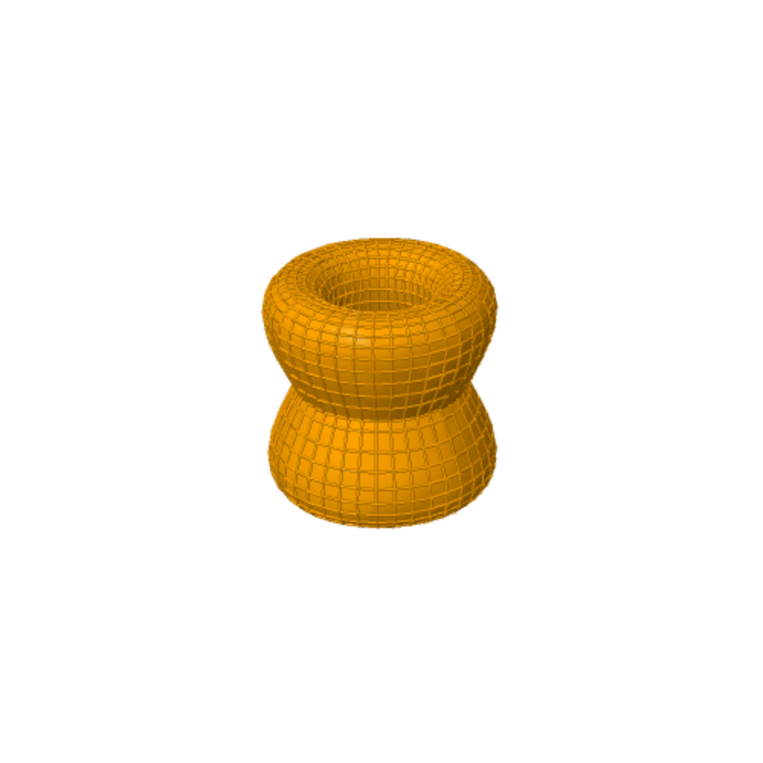
Figure 6: The torus of moduli $(i,\sqrt{2})$.

Communication among different sets (of Monsters) described by an integrated model with a master Lagrangian

Consider a finite covering of $B$ as a compact space such as a compact Riemann surface (or any infinite series of a point which has an accumulation point with identity; Bolzano-Weierstraß theorem; Artin perspective). Therein, the order limit of finite simple groups is at most that of a Monster group (maximizing entropic information while minimizing free energy, Noetherian perspective); i.e., if the order goes beyond the value, it becomes unavoidably not simple and the system will split. This causes $\varnothing=\partial B$ in that situation. For example, take an absolute zeta function $p^{\prime}=s/w$. It belongs to a distribution space of $(\mathscr{D}_{L^{p^{\prime}}})$ and it should be a finite sum of differential coefficients of functions $\in L^{s}$ [Schwartz, 1966]. However, if there is still an infinitely ordered Sato hyperfunction beyond the Schwartz distributions and boundaries [Sato, 1959] [Sato, 1960], communications among different Monsters (analogical to rigid bodies; angular velocity $\Im(s)$ is independent of the coordinate system while translational motion or a fractal dimension $\Re(s)$ is dependent on a particular coordinate system such as an observer; i.e., the nonholonomic world of relativity versus the holonomic world of quantum mechanics) are still possible. These communications render it plausible to bind up the different Monsters to a certain system, in discrete terms, not in the sense of manifolds. Let us consider the match of Steiner circles, or for elliptic integrals considered later as $D$, Poncelet’s poristic polygons including Steiner’s series [Emch, 1899-1900] [Emch, 1900-1901.] in two different Monsters. For the most effective communications, a non-Euclid distance, such as a Lorentz metric, should be selected, multiplied by $\sqrt{-1}$ to accommodate hyperfunctions. The best communication should entail sending out the information of $J(\tau)$ to match the series. Ideally this is between $\Delta(\cong B_{1})$ and $\Delta(\cong B_{2})$ via $\tau=\frac{i\pm\sqrt{7}}{2}$. Here, the Routh function is apparently useful for communication from a particular Monster with a Lagrangian (least action for calculating the trajectory):

$$R(q,p_{m},\xi,\dot{\xi})=p_{m}\dot{q}-L.$$ (167)

As later shown, given a momentum and $q$, $\mathbf{P}=\Im(s)\phi,q=D$, and the relative entropy $S=\ln\Delta\Gamma=\ln\frac{\Delta\mathbf{P}\Delta q}{(2\pi\hbar)^{3}}$ and setting $(2\pi\hbar)^{3}$ as a volume of line integral of action, $k$ becomes uncertainty per volume. The least action is thus connected to maximum entropy. In other words, a least action maximizes a Minkowski metric $s_{M}$ accompanied by $\xi$ to another Monster with a Hamiltonian (energy for a status) accompanied by $q$; e.g., a Carnot cycle of a particular Monster ($M_{C}$) gives work to another Monster ($M_{W}$), the latter sucking up free energy from the former. Dealing with a Frobenioid related to $q$ is straightforward from the viewpoint of Kobayashi (for the étale function, refer to Inter-Universal Teichmüller Theory [Mochizuki, 2020a] [Mochizuki, 2020b] [Mochizuki, 2020c] [Mochizuki, 2020d]). Simply, we took the Dirac picture and $H=H_{0}+H^{\prime}$, where $H,H_{0}$, and $H^{\prime}$ are Hamiltonian, partly independent, and partly dependent of time. $M_{W},M_{C}$ correspond to Hamiltonians of $H_{0},H^{\prime}$. This interaction picture (abbreviated to $I$; the Schrödinger picture is abbreviated to $S$) leads to

$$\ket{\alpha_{I}(t)}\equiv e^{iH_{0S}t}\ket{\alpha_{S}(t)},\beta_{I}(t)\equiv e^{iH_{0S}t}\beta_{S}e^{-iH_{0S}t},i\frac{d}{dt}\ket{\alpha_{I}(t)}=H^{\prime}_{I}\ket{\alpha_{I}(t)},$$ (168)

where $\beta=1/b$ is inverse temperature. For example, if we set $\alpha^{\prime\prime}(\omega)d\omega=\alpha^{\prime\prime}(b)\ket{\alpha_{I}(b)}=\Im(s)D$ and $\omega\alpha^{\prime\prime}(\omega)=\bra{\alpha_{I}(b)}\alpha^{\prime\prime}(b)=\Im(s)D$, $\int_{0}^{\infty}\omega\alpha^{\prime\prime}(\omega)d\omega=\frac{i\pi}{2}\langle\{\dot{\hat{D}}\hat{D}\}\rangle=0$ leads to commutative relation in the Poisson bracket ($=m$ of quantization number). $\pi m/2$ could be a retarded Green function, or from an elliptic function perspective, Legendre’s relation $\eta_{1}\omega_{3}-\eta_{3}\omega_{1}=\pi m/2$. In this case, when the time of $\hat{D}$ is earlier (later) than the time of $\dot{\hat{D}}$, it is non-zero (zero). Generally this is the case with Dictyostelia, excepting Polysphondylium violaceum in November at the Washidu East quadrat. This operation predicts the presence of an irreversible process when the formula is non-zero. If we fix $\hat{D}$, $\dot{\hat{D}}$ starts from the Green function being zero and after it crosses the time for $\hat{D}$, the Green function becomes apparent. Note that in this case, we set $\varepsilon=\mu=D/\Im(s)(=\alpha^{\prime\prime}/\Im(s)^{2})$. The distribution of $\varepsilon,\mu$ in different ratios depending on $\varepsilon\mu=(D/\Im(s))^{2}$ results in a distribution of étale and Frobenioid analogous to the electric and magnetic forces, respectively. When $t\to\infty$, $H(t)=1/2$ and since $m\in\mathbb{Z}$, $\hat{D}^{2}\in 2\mathbb{Z}$, fulfilling the condition for crossing the border $\Re(s)=2$. For further development, some forces analogical to that of physics as inverse square laws, such as gravity and electric fields, can be defined on $D$-space. $M=\phi/\sqrt{1-(H(t)D)^{2}/\Im(s)^{2}}$ is analogical to mass, or electric or magnetic charge. The reason for introducing squares will be discussed later. For the electric force,

$$\mathbf{F}_{e}=\frac{\mathrm{sign}(M)}{4\pi\varepsilon}\frac{M_{i}M_{j}}{D^{2}}\mathbf{e_{F}}$$ (169)

could be defined. Note that the $\mathrm{sign}(M)$ is set at plus when the force acts to increase the number of individuals of particular $M_{i}$, and set at minus when the force acts to decrease the number of individuals of particular $M_{i}$. $i=j$ means self-interaction. Note that $\varepsilon=D/\Im(s)$ in this case. This holds similarly for the magnetic force, with $\mu=D/\Im(s)$. For the gravity force,

$$\mathbf{F}_{g}=\frac{\mathrm{sign}(M)}{4\pi k_{g}}\frac{M_{i}M_{j}}{D^{2}}\mathbf{e_{F}}$$ (170)

could be defined. Note again that the $\mathrm{sign}(M)$ is set at plus when the force acts to increase the number of individuals of particular $M_{i}$, and set at minus when the force acts to decrease the number of individuals of particular $M_{i}$. $i=j$ means self-interaction. Note that $k_{g}=D/\Im(s)$ in this case. Although this is apparently recognizable as a classical Newton equation, note that $k_{g}$ is a function of $D$, not a constant. The gravity, electric, or magnetic force is $\mathbb{R}^{3}\to\mathbb{R}^{2}$ projection of a more generalized form:

$$\mathbf{F}_{s}=\frac{\mathrm{sign}(M)\Im(s)}{4\pi}\frac{M_{i}M_{j}}{D^{3}}\mathbf{e_{F}},$$ (171)

and fixing a single dimension of $D$ as $k_{g}\Im(s)$ or $\varepsilon\Im(s)$ results in the gravity or electric force. Similar logic also applies for the magnetic force.

Now consider a Schwarzschild solution analogy to a black hole. The entropy of the solution would be $S_{BH}=c^{3}A/4G=\pi D4\pi(\Im(s)D)^{2}$, which represents a $\pi D$ increase of a sphere with radius $\Im(s)D$. The Planck-length is $\ell_{P}=1/\sqrt{4\pi D}$. The information of this solution is roughly accumulated in this minimal surface. The Schwarzschild radius is $r_{H}=2GM=\Im(s)M/2\pi D$ and it is a quotient of a momentum $\Im(s)M$ to a circumference $2\pi D$. The Hawking temperature is $T_{H}=\frac{1}{8\pi GM}=\frac{\pi D}{2\Im(s)M}$. Thus, species $M$ is accompanied by this trapping radius and a temperature analogical to the black hole. Jeans wave number $k_{J}$, wave length $\lambda_{J}$, and mass $M_{J}$ would be

$$k_{J}=\sqrt{\frac{N_{k}\Im(s)}{bD}},\lambda_{J}=2\pi\sqrt{\frac{bD}{N_{k}\Im(s)}},M_{J}=\frac{4}{3}\pi^{4}\sqrt{\frac{1}{N_{k}}(\frac{bD}{\Im(s)})^{3}}.$$ (172)

Perturbations larger than $\lambda_{J},M_{J}$ would admit developments of species dynamics (Tables 16 - 19). This analogy to celestial objects is developed into an H-R plot of species (Figure 7). There are three distinct phases: $b$ values under $\sim 300$ denoting a chaotic situation, $b$ values above $\sim 700$ with an upper distribution ($N>600$) for an adapted situation, and $b$ values above $\sim 700$ with a lower distribution ($N<200$) denoting a disadapted situation. This type of plot is useful to discriminate the phase of the species.

Table 16: $\lambda_{J}$ values compared to $D$ (Washidu East).

$\lambda_{J}$	P. pallidum	D. purpureum	P. violaceum	D	P. pallidum	D. purpureum	P. violaceum
April				April
June	2.358	0.4255	1.852	June	1.005	1.013	1.009
July				July
August				August
September	1.472	5.324		September	1.003	1.003
October	1.100	6.623		October	1.003	1.003
November	2.253		0.2943	November	1.013		1.036
December				December
January				January

P. pallidum: Polysphondylium pallidum; D. purpureum: Dictyostelium purpureum; P. violaceum: Polysphondylium violaceum. Numbers in red indicate perturbations larger than $\lambda_{J}$. Blank cells signify not calculable.

Table 17: $\lambda_{J}$ values compared to $D$ (Washidu West).

$\lambda_{J}$	P. pallidum	D. purpureum	P. violaceum	D	P. pallidum	D. purpureum	P. violaceum
April				April
June				June
July	1.634	2.703	0.3881	July	1.006	1.003	1.008
August	1.476	5.127		August	1.002	1.002
September	0.7980	1.752	4.556	September	1.003	1.003	1.000
October	1.478		5.158	October	1.003		1.003
November				November
December				December
January				January

P. pallidum: Polysphondylium pallidum; D. purpureum: Dictyostelium purpureum; P. violaceum: Polysphondylium violaceum. Numbers in red indicate perturbations larger than $\lambda_{J}$. Blank cells signify not calculable.

Table 18: $M_{J}$ values compared to $N$ (Washidu East).

$M_{J}$	P. pallidum	D. purpureum	P. violaceum	N	P. pallidum	D. purpureum	P. violaceum
April				April		75.56
June	841.7	8.423	174.5	June	122.6	208.9	52.44
July				July	1282
August				August	1561
September	1504	8429		September	900.6	106.7
October	745.3	5289		October	1069	34.78
November	359.1		1.345	November	60.00		100.8
December				December	189.6
January				January	28.90

P. pallidum: Polysphondylium pallidum; D. purpureum: Dictyostelium purpureum; P. violaceum: Polysphondylium violaceum. Numbers in red indicate perturbations larger than $M_{J}$. Blank cells signify not calculable.

Table 19: $M_{J}$ values compared to $N$ (Washidu West).

$M_{J}$	P. pallidum	D. purpureum	P. violaceum	N	P. pallidum	D. purpureum	P. violaceum
April				April		82.67
June				June	146.7
July	182.6	2220	9.795	July	80.00	214.8	320.0
August	2241	12760		August	1330	180.78
September	215.3	216.8	32130	September	809.2	77.00	648.9
October	1350		7666	October	798.8		106.7
November				November	335.6
December				December	711.1
January				January	99.00

P. pallidum: Polysphondylium pallidum; D. purpureum: Dictyostelium purpureum; P. violaceum: Polysphondylium violaceum. Numbers in red indicate perturbations larger than $M_{J}$. Blank cells signify not calculable.

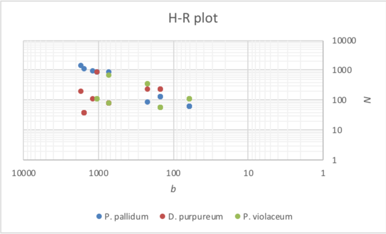
Figure 7: Phase diagram for species.

For further investigation, consider an analogue of radius of action in the nuclear force, ${\mkern 0.75mu\mathchar 22\relax\mkern-9.75mu\lambda}\approx\frac{\hbar}{Mc}=\frac{1}{M\Im(s)}$ and as $D\sim 1$ we can set ${\mkern 0.75mu\mathchar 22\relax\mkern-9.75mu\lambda}r_{H}=1$. Thus when $D>r_{H}$, there is an interaction between the Monsters analogous to a Schwarzschild black hole, which is likely to be involved in Yukawa-type potential. When $D\leq r_{H}$, it is not possible to get outside the Monster. If $r_{H}\ll 1$, there is an attraction force to develop the fractal dimension.

Furthermore, considering an inverse cube of $\frac{1}{3}\Im(s)D$ results in a case similar to quantum color dynamics (QCD) (equals the average of the square of a radius of gyration). With an analogue of color as $C=\sqrt{\frac{1}{3}}(R\bar{R}+G\bar{G}+B\bar{B})$, $\exp(C)^{2}=\exp(\frac{1}{3}(\Im(s)D))^{3}$ results in $\Im(s)D=(R\bar{R})^{2}+R\bar{R}G\bar{G}+B\bar{B}R\bar{R}$, or a permutation with $R,G,B$, in the sense of a QCD analogue. Color thus becomes valuation of interacting particles. Three-body interaction of $\Re(s)=2$ (hence, with $\Re(s)=-2$ as future) and $\Re(s)=5$ is an example of the case. This $l=5$ case should be regarded as two different aspects. We can consider $\tau_{\rho}=\frac{1}{12}(\frac{1}{4}-\rho^{2})\equiv 2(1+\rho^{2})(\mod 5)$ as in [Mochizuki, 1999]. $\rho=0$ results in $\bar{\mathcal{N}}_{1,1}^{0}$ being divided to $2$ over $\bar{\mathcal{M}}_{1,1}$ and $3$ over $\bar{\mathcal{M}}_{1,1}$; this is an aspect from the same layer as the observant, consisting of $l=2,2,3$ as the three bodies. Similarly, $\rho=1$ results in $\bar{\mathcal{N}}_{1,1}^{1}$ being divided to $1$ over $\bar{\mathcal{M}}_{1,1}$ and $3$ over $\bar{\mathcal{M}}_{1,1}$ (reduced); this is an aspect from the same layer as the observer, observing $\Re(s)=4\to 3$ from $1$. On the other hand, $\rho=\pm i$ results in $\bar{\mathcal{N}}_{1,1}^{-1}\cong\bar{\mathcal{N}}_{1,0}$; this is an aspect from the upper layer from the layer of the observer. In the latter case, the constituents of $l=2+3=5$ can be regarded as forming a solitary acting on the original $l=2$ constituent.

For further clarification, consider D-fivebranes superstring theory [Witten, 1995] [Lambert, 1998]. $\mathbb{R}^{4}(3+1)$ case would develop one-number ADHM instanton [Witten, 1995], and the potential energy is $V=\frac{1}{8}(X^{2}+\rho^{2})\phi^{2}$. Our case implies $(X,\phi)=(1,4)$ and $\rho$ is either $0$ with a branch, $1$ for normal observation, or $\pm i$ with a fractal. A massless model would result in D-fivebranes $\Re(s)=5$ with type I or type IIA, B superstring theory with $K3\times S^{1}$ [Lambert, 1998] ($11-5=6$ dimensions compactified on M-theory). Since a $K3$ surface might be related to the $M_{24}$ group as a subgroup, $M_{24}$ is related to our model in the sense of condensed matter physics described by superstring theory.

This D5 system is analogical to the D1-D5 system in [Martinec et al, 1999]. When $H_{i}=1+(\frac{q_{i}}{D})^{2},i=1,5;h=1-(\frac{r_{H}}{D})^{2}$, the Lorentz metric is

$$ds_{M}^{2}=\frac{-hdt^{2}+dD_{5}^{2}}{\sqrt{H_{1}H_{5}}}+\sqrt{\frac{H_{1}}{H_{5}}}dD_{||}^{2}+\frac{h^{-1}dD^{2}+d\Omega_{3}^{2}}{\sqrt{H_{1}H_{5}}}.$$ (173)

Sending the length of string $l_{s}=2\pi l\to 0$ (as observant) would result in

$$\frac{ds_{M}^{2}}{l_{s}^{2}}=\frac{-hdt^{2}+dD_{5}^{2}}{\sqrt{g_{s}^{2}Q_{1}Q_{5}}}(\frac{D}{l_{s}^{2}})^{2}+\sqrt{\frac{Q_{1}}{Q_{5}}}[\frac{dD_{||}^{2}}{V_{4}^{1/2}}]+\frac{h^{-1}(\frac{dD}{D})^{2}+d\Omega_{3}^{2}}{\sqrt{g_{6}^{2}Q_{1}Q_{5}}},$$ (174)

with $Q$ being an instanton and $V_{4}=\Sigma_{1}\Sigma_{2}\Sigma_{3}\Sigma_{4}$. The geometry is locally $AdS_{3}\times S^{3}\times T^{4}$, the radius of $S^{3}$ is $R_{AdS}=l_{s}(g_{6}^{2}Q_{1}Q_{5})^{1/4}$, and the characteristic proper size of $T^{4}$ is $l_{s}(Q_{1}/Q_{5})^{1/4}$. This would lead to a harmonic function

$$H=\sum_{\alpha}\frac{q_{\alpha}^{2}}{|D/D_{\alpha}|^{2}},h=0;(D\sim r_{H})$$ (175)

as the inverse square law when $M_{\alpha}=q_{\alpha}$.

Physical Lagrangian densities for quantum electrodynamics (QED) and QCD are

$$\mathfrak{L}=\bar{\psi}(ic\gamma^{\mu}\partial_{\mu}-Mc^{2})\psi+e\bar{\psi}\gamma^{\mu}A_{\mu}\psi-\frac{1}{4\mu_{0}}F_{\mu\nu}F^{\mu\nu},$$ (176)

$$\mathfrak{L}=\bar{q}(ic\gamma^{\mu}\partial_{\mu}-Mc^{2})q+g(\bar{q}\gamma^{\mu}T_{a}q)G_{\mu}^{a}-\frac{1}{4}G_{\mu\nu}^{a}G_{a}^{\mu\nu}.$$ (177)

In the sense of Lefschetz operator ($i\bar{\partial}$) for multiplication, this is in the form

$$\mathfrak{L}=\frac{1}{2}(\partial_{\mu}\phi_{i})^{2}-\frac{1}{2}\mu^{2}\phi_{i}^{2}-\frac{1}{4}\lambda(\phi_{i})^{4}.$$ (178)

A counterpart of these in integrated form in our model is

$$\mathfrak{L}=\frac{1}{2}(-sw\Im(s)-M\Im(s)^{2})\phi_{i}^{2}+\frac{1}{2}p^{2}\phi_{i}^{2}-\frac{1}{4}l\frac{\Im(s)}{D}(\phi_{i})^{4}.$$ (179)

The first term is diminishing mass, the second is the remaining Frobenioid, and the third is the contribution to fractals. $\phi_{i}$ would be Selberg zeta $\zeta_{\Gamma}$, Hasse-Weil $L$ or a field $|\mathbf{f}_{s}|=\frac{\Im(s)}{4\pi}\frac{M}{D^{3}}(s\to\Re(s),w\to\Re(s)-1)$ as indicated earlier (Tables 20 -22). Empirically, $H(t)\approx 0$ and the effect of this parameter is neglected. For a Hamiltonian, they are significantly low when black hole analogies are prominent. For a Lagrangian, negative values may indicate a contribution to fractals composed by climax species Polysphondylium pallidum, while positive values may be anti-fractal species dynamics attributable to pioneering species Dictyostelium purpureum & Polysphondylium violaceum (refer to [Adachi, 2015]).

Table 20: $|\mathbf{f}_{s}|$ values.

$|\mathbf{f}_{s}|$	WE P. pallidum	WE D. purpureum	WE P. violaceum	WW P. pallidum	WW D. purpureum	WW P. violaceum
April
June	0.2045	6.189	0.3291
July				0.3998	0.1470	7.049
August				1.575	0.1307
September	1.638	0.1253		2.211	0.4583
October	3.484	0.09617		1.575		0.1294
November	0.2209		12.38
December
January

WE: Washidu East quadrat, WW: Washidu West quadrat; P. pallidum: Polysphondylium pallidum; D. purpureum: Dictyostelium purpureum; P. violaceum: Polysphondylium violaceum. Numbers in red indicate significantly large values deduced by a black hole analogy. Blank cells signify not calculable.

Table 21: Lagrangian.

$\mathfrak{L}$	WE P. pallidum	WE D. purpureum	WE P. violaceum	WW P. pallidum	WW D. purpureum	WW P. violaceum
April
June	-0.3983	7.609E+5	-5.164
July				5.676	-0.08279	1.907E+6
August				-899.8995563	-0.800427157
September	-1072	-0.9108		-2036	2485
October	-2.368E+4	-2.932		-906.8		-0.8065
November	-0.4868		2.820E+7
December
January

WE: Washidu East quadrat, WW: Washidu West quadrat; P. pallidum: Polysphondylium pallidum; D. purpureum: Dictyostelium purpureum; P. violaceum: Polysphondylium violaceum. Numbers in red indicate significantly large absolute values deduced by a black hole analogy. Blank cells signify not calculable.

Table 22: Hamiltonian.

$\mathfrak{H}$	WE P. pallidum	WE D. purpureum	WE P. violaceum	WW P. pallidum	WW D. purpureum	WW P. violaceum
April
June	-0.4346	-1.230E+6	-10.24
July				-39.89	-0.1037	-2.707E+6
August				-684.2	-0.8629
September	-798.1	-0.9680		-5601	-2686
October	-1.278E+4	-4.487		-690.0		-0.8678
November	-0.5288		-3.558E+7
December
January

WE: Washidu East quadrat, WW: Washidu West quadrat; P. pallidum: Polysphondylium pallidum; D. purpureum: Dictyostelium purpureum; P. violaceum: Polysphondylium violaceum. Numbers in red indicate significantly large absolute values deduced by a black hole analogy. Blank cells signify not calculable.

The energy

$$E=\sum_{k}\frac{\partial\mathfrak{L}}{\partial\dot{q}_{k}}\dot{q}-\mathfrak{L}=\mathfrak{H}=\frac{1}{2}(-sw\Im(s)-M\Im(s)^{2})\phi_{k}^{2}-\frac{1}{2}p^{2}\phi_{k}^{2}+\frac{1}{4}l\frac{\Im(s)}{D}(\phi_{k})^{4},$$ (180)

and

$$p_{k}=\frac{\partial\mathfrak{L}}{\partial\dot{q}_{k}}=\frac{-sw\Im(s)-M\Im(s)^{2}}{H(t)D}\phi_{k}^{2}.$$ (181)

$\dot{q}_{k}=p_{k}/M$ and

$$D=\frac{i}{H(t)}\sqrt{\frac{sw\Im(s)}{M}+\Im(s)^{2}}\cdot\phi_{k}.$$ (182)

The sign is for a weak interaction analogue and it completely depends on environmental factors in our biological model. This completes our integrated model for biology analogical to the standard model plus gravity theory, investing a single dimension with a topology to a dynamical system with a Lagrangian and Hamiltonian.

Further clarification of our model

If we regard $D=u-w=K$ as an elliptic integral, $f(u)=\sum\frac{1}{D_{i}^{3}}$ has dual periodicity and Weierstraß $\wp=-\zeta^{\prime}(z;\Lambda)$, where Weierstraß zeta would be $\zeta(z;\Lambda)=\frac{1}{z}+\sum_{w\in\Lambda^{*}}(\frac{1}{z-w}+\frac{1}{w}+\frac{z}{w^{2}})$. Weierstraß zeta accounts for observations from multiple $w$ and $0$ accompanied with an absolute zeta function from duplications of $w$. Furthermore, a set of differentials of the first kind of $K$, $\mathfrak{L}_{0}\ni w_{i}dz$, and one-dimensional topologically congruent group $B_{1}^{*}(\mathfrak{R})$ with real coefficients become isomorphic as a $k_{0}$-module. An Abel-Jacobi map shows that

$$\bar{\mathfrak{D}}_{0}:=\mathfrak{D}_{0}/\mathfrak{D}_{H}\cong V_{g}(k)/P(w_{i}dz).$$ (183)

$\mathfrak{D}_{0}$ is a $0$-dimensional factor group of $K$ and $\mathfrak{D}_{H}$ is a principal factor group of $K$. $D$ could be regarded as a periodic group, $P(w_{i}dz)$. Thus $\mathfrak{D}_{H}\cong P(w_{i}dz)$. A $g$-dimensional complex vector module of a modulus $k$, $V_{g}(k)\cong\mathfrak{D}_{0}$, could be $\mathrm{sign}(M_{i})M_{i}$ ($M_{i}$ can be $\Im(s)$). Neglecting factorization by a solid angle $4\pi$, the inverse square law could be multiplication of three $\bar{\mathfrak{D}}_{0}$ in the Abel-Jacobi map.

Interestingly, calculation using physical values from 2018 CODATA shows $\sqrt{k_{g}\sqrt{\varepsilon_{0}\mu_{0}}}\sim 1.9943\sim 2$, and $\mathbf{F}_{s}=\frac{\mathrm{sign}(M)}{8\pi}\frac{M_{i}M_{j}}{D^{2}}\mathbf{e_{F}}$, fulfilling equal partition of forces to outward and inward directions of a particular sphere with radius $D$. This also suggests the branching of the gravity force occurred first, and the branching of the electric (communicative “étale”) from the magnetic force ($=4\pi\times 10^{-7}$ and thus a Frobenioid) occurred afterwards. The subtle difference from $2$ value indicates neglecting the effect from weak interaction, whose calculation is not straightforward in our model. Even in the standard model, a neutrino is massless and this differs from empirical understandings.

For the SI unit system, the dimension of this value is $\mathrm{\frac{\sqrt{kg\cdot s^{3}}}{m^{2}}}$. In our unit system, it is dimensionless. The constant would be $\frac{\sqrt{\phi}t^{3}}{D^{2}}$. The measure of root of observed $\phi$, $\sqrt{\phi}$, is equivalent to $t$ (a root of physical time), and the measure of $D$ is a square of $t$, indicating observation linked to interaction. That is, a multiplication of a root of the observant and a cube of $t$ is a duplication of observed fitness of $D^{2}$, indicating duplicated fitness in the potential cube-$t$ space. For further development, considering Einstein’s equation

$$R_{ik}-\frac{1}{2}g_{ik}R=\frac{8\pi G}{c^{4}}T_{ik},$$ (184)

where $G=1/8\pi,c=\Im(s),T_{ik}=\phi\Im(s)^{2}D^{2}\sqrt{\frac{\Im(s)^{2}+(H(t)D)^{2}}{\Im(s)^{2}-(H(t)D)^{2}}},\dot{D}=H(t)D$, and the curvature of the left-hand side equals to $\phi\cdot(\frac{\dot{D}}{H(t)\Im(s)})^{2}\cdot\sqrt{\frac{\Im(s)^{2}+(H(t)D)^{2}}{\Im(s)^{2}-(H(t)D)^{2}}}$. This means, if the system is abstracted to a sphere, $1/r^{2}=\phi\cdot(\frac{\dot{D}}{H(t)\Im(s)})^{2}\cdot\sqrt{\frac{\Im(s)^{2}+(H(t)D)^{2}}{\Im(s)^{2}-(H(t)D)^{2}}}$ and $r=H(t)\Im(s)/\dot{D}\sqrt{\phi\sqrt{\frac{\Im(s)^{2}+(H(t)D)^{2}}{\Im(s)^{2}-(H(t)D)^{2}}}}$. It is also notable that the Ricci curvature tensor is a multiplication of the metric tensor of $1$ and the ratio of étale to Frobenioid, i.e., the determinant with matrix from the second fundamental form to that from first fundamental form. The resultant term appears as $\phi\cdot(\frac{\dot{D}}{H(t)\Im(s)})^{2}\cdot\sqrt{\frac{\Im(s)^{2}+(H(t)D)^{2}}{\Im(s)^{2}-(H(t)D)^{2}}}$, and $t\to\infty,\Im(s)\gg H(t)D$ leads to $4\phi(\dot{D}/\Im(s))^{2}$.

The Macdonald formula shows

$$\prod_{m=1}^{\infty}(1-q^{2m})^{k}=\sum_{m=0}^{\infty}a_{m,k}q^{m}.$$ (185)

If $\mathfrak{g}=\mathfrak{sl}_{2}$, then $k=3$ and it becomes

$$\sum_{m=-\infty}^{\infty}(-1)^{m}(2m+1)(q^{m(m+1)})=2\prod_{m=1}^{\infty}(1-q^{2m})^{3}.$$ (186)

Regarding $D_{m}^{-1}=(1-q^{2m})$, a whole product of infinite $D$ results in multiplication of the value by $2$, similar to the situation above. Regarding bosonic fitness $w$, $2m+1$ means a chaotic situation and this underlies the inverse square law, if the forces are not multiply split.

It is notable that by introducing a squared part for mass, $H(t)D>\Im(s)$ means the mass becomes a purely imaginary number, not a real number. The dimension for the potential as an imaginary axis thus rotates when multiplied by $-i$, and it becomes a real axis. Thus, the potential could be converted to a fractal dimension and it becomes apparent when the velocity of increasing $D$ is high enough such that $H(t)D>\Im(s)$, which is true for zero points of a Riemann zeta function as expected. When the velocity is approximately $\Im(s)$, the first-order approximation for kinetic energy is $\frac{1}{2}M\Im(s)^{2}$. This is achieved in $E=M\Im(s)^{2}$ energy theory when $(H(t)D)^{2}=5\Im(s)^{2}$. Thus, for creating fractals beyond $\Re(s)=2$ (square law), one needs recognization from $5$-dimensioned fractals in each for $H(t)D\approx\Im(s)$. This is useful for between $\Re(s)=5$ and $\Re(s)\sim 2$ for the development of fractals. The energy related to these forces means energy for creating fractals. For example, recall $s=\frac{\sqrt{7}+i}{2}$ as indicated earlier. The self-interaction of $s$ results in $\frac{7}{4}e_{\Re(s)}^{2}+\frac{2\sqrt{7}}{4}ie_{\Re(s)}e_{\Im(s)}-\frac{1}{4}e_{\Im(s)}^{2}$. Thus, the weight for the first term is $\frac{4}{7}$ and it should be an integer. The second term is not an integer and the third term is a multiple of $4$, and neither of them should be considered further. For the Pontryagin class (or, a part of the Hirzebruch signature as indicated), $p_{2}(M)=\frac{4(2i-1)^{2}+45}{7}$ and the first term corresponds to $p_{2}(M)$ as $\Re(s)=2i-1\ (p_{1}(M)=2(2i-1))$. If the condition $i\equiv 0,1\mod 7$ is fulfilled, then $p_{2}(M)$ is an integer and $M$ is a differential manifold. However, if not, $M$ is an exotic sphere that is homeomorphic but not diffeomorphic to the standard Euclidean $S^{7}$. For a continuous time model by differentials, this is not allowed and development into $\Re(s)\geq 5$ should be achieved in partners of $\Re(s_{1})+\Re(s_{2})=7j,7j+1,j\in\mathbb{N}$ (e.g., $\Re(s)=5$ and $\Re(s)=2$ observed in October at the Washidu East quadrat between Polysphondylium pallidum  and Dictyostelium purpureum ).

Roles of another analogy to quantum mechanics in our model

If we set $\phi\ket{\alpha_{S}(t)}=l\ket{\alpha_{S}(t)}$ and $\bra{\alpha_{S}(t)}\phi=\bra{\alpha_{S}(t)}p$, then the bra becomes the basic bra and the ket becomes the standard ket. The former represents phase information (Frobenioid; persistence homology), and the latter represents the norm (étale function or cohomology). Note that $l$ is suitable for communication because of its characteristics beyond the restricted layer of a particular system. Setting the $\Phi(\alpha)=0$ function as a monic polynomial for a cyclotomic field, the polynomial becomes a zero ideal of the ring structure for the bra or ket. The eigenvalues for $\ket{\alpha(t)}\bra{\alpha(t)}$ are either 1 or 0 (an observed state or non-observed state by the interactions between a particular set of kets and bras), and this information is usable for Morse code for the communication. Their integration becomes a Dirac $\delta$ function, that is, $\Re(s)=l$. Only where $p=l$, $\bra{\alpha(t)}\phi\ket{\alpha(t)}$ leads to $E(N)$. For the $H=H_{0}+H^{\prime}$ case of $M_{C}$ and $M_{W}$, $H_{0}=l$, $H^{\prime}=-l$, and $H=l+(-l)=0$. This means $M_{W}$ is invested with a fractal structure of $l$-dimensions, while $M_{C}$ loses the same number of fractal dimensions. The time development will result in a static state of $M_{W}$ being invested with everything if the relation continues at all.

The entanglement entropy of these two harmonic oscillators is

$$S_{A}=\cosh^{2}\theta\ln\cosh^{2}\theta-\sinh^{2}\theta\ln\sinh^{2}\theta,$$ (187)

where $\theta$ is expressed by $l=\frac{2\sinh\theta\cosh\theta}{1+2\sinh^{2}\theta}$ with Hamiltonian $H=w^{{\dagger}}w+c^{{\dagger}}c+l(w^{{\dagger}}c^{{\dagger}}+wc)$, when $(w,w^{{\dagger}}),(c,c^{{\dagger}})$ are creation-annihilation operators of $M_{W},M_{C}$. For maximum entanglement, consider Hilbert spaces $\mathcal{H}_{W},\mathcal{H}_{C}$. The dimensions of the spaces are $|\mathcal{H}_{W}|=\sum N_{W},|\mathcal{H}_{C}|=\sum N_{C}$ and $\min(\ln|\mathcal{H}_{W}|,\ln|\mathcal{H}_{C}|))$ is their maximum entanglement entropy. If $M_{W}$ absorbs all of $N_{k}$ in $M_{C}$, then $\ln|\mathcal{H}_{C}|=\ln P+N_{k}\frac{s}{b}$ and the second term approaches zero. Thus, $\ln P$ is the entanglement entropy attributable to diminishing $N_{k}$.

It is notable that once assuming an analogy to QED of the Frobenioid-étale relationships, at least for $\Re(s)=2,3$, hetero-interaction terms become negligible according to QED, which accords well with empirical results. For the most efficient communication that communicates all the étales and Frobenioids, as both of them are in parallel, the following condition is needed:

$$\frac{\frac{\mathbf{V}}{\Im(s)}}{1+\frac{\mathbf{V}^{2}}{\Im(s)^{2}}}=\frac{\mathbf{\mathbf{E}\times\mathbf{H}}}{E^{2}+H^{2}}$$ (188)

[Landau and Lifshitz, 1975]. Along this line, a conservation law in $D$-space could be

$$\frac{\partial}{\partial t}\Biggl{\{}\frac{E^{2}+H^{2}}{2}dV+\sum\mathscr{E}_{\mathrm{kin}}\Biggr{\}}=-\oint\mathbf{S}d\mathbf{f}(=0),$$ (189)

where a Poynting vector $\mathbf{S}=\Im(s)\mathbf{E}\times\mathbf{H}$ and $d\mathbf{f}$ is an areal element. $(=0)$ is achieved when the volume is infinite.

From renormalization to fractals

Furthermore, in our biological model, we can attribute hierarchical formation to the solution for the divergence problem of transition probability, as of renormalization. Terms of harmonic oscillators for a Hamiltonian of QED become divergent unless renormalized. However, we can treat each of the oscillators as an additional dimension of a fractal structure. Mathematically, the plausibility of renormalization as $P^{m}$ would be defined as the existence of $0\in U$, $(P^{m},U,V)$ being a mapping similar to a quadratic and a filled Julia set $K_{m}$ being connected, when the quadratic $P(z)=z^{2}+c$ and $U,V$ are simply connected regions. The condition is fulfilled in a continuously developing system constituted by components of simply connected regions with an observant $U$ in our case. The renormalization equation would be

$$\mu\frac{d\mathfrak{M}}{d\mu}=\Biggl{(}\mu\left.\frac{\partial}{\partial\mu}\right|_{e}+\mu\frac{\partial e}{\partial\mu}\frac{\partial}{\partial e}\Biggr{)}\mathfrak{M}=0.$$ (190)

The first and second terms on the left-hand side are renormalizing and remaining terms, respectively. These have negative and positive values, and represent the contribution of $\mathfrak{M}$ to fractal structure. Or, we may state that a fractal $l$-dimension is for one of the periods of an elliptic function that acts on a “string”.

However, the plausibility of renormalization is restricted to $d<8$, at most, in the $\mathbb{R}^{3}\times\mathbb{R}^{3}\cong\hat{\mathbb{C}}$ case. For further application, a similar statement is true for the Bogomolov conjecture. Let $A$ be an abelian manifold on an algebraic field $K$. Let $L$ be a symmetric and enriched invertible sheaf on $A$ and $A_{\bar{K}}:=A\times_{\mathrm{Spec}(K)}\mathrm{Spec}(\bar{K})$. $X$ would be an irreducible algebraic submanifold of $A_{\bar{K}}.$When $\hat{h}_{L}$ is a Néron-Tate height function on $L$ and $\forall\varepsilon>0$, a set $\{x\in X(\bar{K})|\hat{h}_{L}(x)\leq\varepsilon\}$ is dense in the sense of Zariski topology in $X$, there exists a subset of an abelian manifold $B$, and a torsion point $b$ on $A_{\bar{K}}$ s.t. $X=B+b$. Regarding $b$ as analogical to the term for renormalization, one can simply consider $B$ for the current layer and $b$ is a partial point of fractals, or a fractal string. That is, $B$ is a Frobenioid and $b$ is an étale.

3 Discussion

Our main results

To the best of our knowledge, no previous studies have considered the biological view proposed herein. We introduce an index, small $s$, to distinguish between populations and species ($\Re(s)=\frac{\ln\frac{N_{1}}{N_{k}}}{\ln k}$ when $N_{1}$ and $N_{k}$ is a population density of first, $k$-th rank, $k\neq 1$ and $\Re(s)=\zeta^{-1}(E(\Sigma N)/N_{1})$ when $E(\Sigma N)$ is an expected population density, $k=1$ and $\zeta^{-1}$ is an inverse of Riemann zeta function; $\Im(s)=e^{E(\Sigma N)\Re(s)/b}$ when $b$ is an approximation parameter of $N_{k}=a-b\ln k$); the value of the real part of this index is high for an ordered species and low for a fluctuating population in the wild; that is, $\Re(s)=2$ is a critical line for both, in strong agreement with fractal theory of a box dimension $\dim_{B}A=2$ with a model $\mathbb{R}^{2}$, which is the case for our $s$ metric. To begin, we modified the Price equation [Price, 1970] to develop our index, small $s$, which is based on the $R=T$ theorem and Weil’s explicit formula [Weil, 1952] [Taylor and Wiles, 1995] [Wiles, 1995]. The Price equation describes evolution and natural selection, and here it is used to replace gene frequencies with the proportion of individuals in a given population or species. The small $s$ index is related via covariance and expectation to the Price equation. The nontrivial zeros of the Riemann $\zeta$ function provide information about the bursts or collapses of a population. In this model, speciation is thus related to prime numbers; that is, a prime ideal indicates the status of a specific species in the system, and time-dependent multiplication of the fitness can be calculated by utilizing these primes. We then calculate the unique equations of the model in the Maass form and examine the spectra of the data. Use of the Selberg zeta and Hasse-Weil $L$ to calculate the norm of prime closed geodesics $|N(p)|$ clarifies that the noninteracting adaptive species world (an integrative space of time and other dimensions) is in the mode $|N(p)|=2/3$, while the interacting neutral populations are in the mode $|N(p)|=1$. Combining these calculations with phylogenetical asymmetry, we determine whether the observed hierarchy of data represents chaotic populations/nonadaptive species or adaptive species in genuinely successful niches. Our model has been partially successful at predicting imminent transitions between biological phases (adaptation/disadaptation). By utilizing the Schwarz equation, we also determined the time-dependent fitness function that matches the observations. Additionally, web-based formalism [Gaiotto et al., 2016] based on a combination of supersymmetry (Hodge-Kodaira decomposition of a non-degenerate fermionic $\phi$ function) and an analogy to the transactional interpretation of quantum mechanics leads to a nine-dimensional model without time (three-dimensional nature $\times$ three-dimensional fluctuations). The idea of a fitness space leads to a precise time-dependent Hubble parameter for that space, for an appropriate timescale. Finally, the nature of asymmetric time development of $\phi$ within our model is elucidated, and a degenerate $\psi$ (fitness-related) function also deduces some aspects of future. The proposed model combines information theory and observations from nature to bring new understanding to the biological ideas of population and species; this is different from the physical and theoretical thermodynamical approach used by [Volkov and Banavar, 2004]: our model is nothing related to physical dynamics. Analogy to physics is performed in biological scale, not physical scale. Here, a patch is defined to be a small plot or piece of land, especially one that produces or is used for growing specific organisms. We call our model the patch with zeta dominance (PzDom) model, and it is only necessary to evaluate $\Re(s)$ to determine whether a population is chaotic or dominated by species; the border is at $\Re(s)=2$. That is, sometimes species dynamics is seen and The model requires only the change in density of individuals over time. We will also discuss the significance of biological hierarchies. We propose an approach that will allow future research to explore the nature of hierarchical systems.

Our model interpreted by information theory

We propose an original model that uses a different definition of entropy (relative entropy, i.e., $\ln k$ when $k$ is the rank of population number; this is equivalent to relative entropy as a Kullback-Leibler divergence, $D_{1}(P||Q)=\sum_{i=1}^{n}p_{i}\ln\frac{p_{i}}{q_{i}}$ of $n=1,p_{i}=1,q_{i}=1/k$) than that used by [Harte et al., 2008] and a new definition of temperature: an integrative environmental parameter that determines the distribution of population/species deduced from the logarithmic distribution of populations/species. The units of this parameter are set to cells/g, and it is a half-intensive parameter, as described in the first parts of Results. We define new metrics that are based on statistical mechanics [Fujisaka, 1998] [Banavar et al., 2010] [Tasaki and Hara, 2015] to distinguish and interpret species and population counts in mixed communities; we apply this to an actual community of Eastern Japanese Dictyostelia [Adachi, 2015]. The use of statistical mechanics to interpret biological systems began with [Lotka, 1922], proceeding to the disastrous complexity of the Hamiltonian described by [Kerner, 1957], and continued with the Lotka-Volterra equations of N-interacting species in an artificially noisy environment [Spagnolo et al., 2004]. [Kerner, 1957] also posited an interesting model for a time-developing system; however, Kerner’s model and our model belong to different mathematical spaces, and a set of mathematically rigorous studies is required to precisely describe their interrelationships. This is different from a time-dependent ecosystem assembly model that is restricted to finite Markov chains, such as was proposed by [Pigolotti et al., 2005] or [Capitán et al., 2009]. We will describe the nonrandom directionality of the model, which is based on number theory with $|N(p)|=2/3$. Importantly, we are able to calculate the different sets of critical temperatures and Weiss fields (with Bose-Einstein condensation) at which various natural first-order phase transitions take place among species or populations (where by ‘phase transitions’ we mean a community moves from chaos caused by neutrality or nonadaptive situations and results in an increase of or domination by a particular species, or moves from that to domination by a particular population within a species). The order parameter in this model is large $S$. This complex phase transition nature of different hierarchies in the wild was not fully explained by [Harte et al., 2008]; it was briefly mentioned by [Banavar et al., 2010] as part of the relative entropy. The model shows that the populations of some highly adapted species are much more stable than those of others.

Application of our model other than Dictyostelia

In our PzDom model, under the effects of entropy, the populations/species are assumed to fluctuate for $\Re(s)\sim 1$ or $\zeta=0$. However, there is another solution. From the fractal theory results shown in Figure 1, $\Re(s)=2$ is the border between population and species for Dictyostelia in the box dimension of the system. In the ecological data set of ruderal vegetation presented by [Rodríguez et al., 2013], we can deduce that the data pertain to opportunistic species because in most areas $\Re(s)>2$. On the other hand, marine interstitial meiofauna on sandy beaches and tropical rocky shore snails should be from populations, or at least from equilibrium species, because of $\Re(s)<2$. As discussed above, adaptation can be defined as fitness that is sufficient to go beyond the fluctuations of harmonic neutrality and the border to this region is at $\Re(s)=2$. From the data, we also observe that species with larger values of $s/D$ have greater fitness. Since the world in which $\Re(s)>1$ results in absolute convergence of $\zeta$, the species world is not a chaotic world, but there is structure in the community that depends on adaptation and hysteresis. It is obvious that from the original Price equation, $\Re(s)>1$ means $\mathrm{Cov}>0$ and thus such a species/population is on a course of diverging characteristics. When $0<\Re(s)<2$, it is chaotic characterized by $<\tilde{\mathscr{R}}_{A,\Omega}^{[k]},\varphi>$. It is also obvious that from the original Price equation, $\Re(s)<1$ implies that $\mathrm{Cov}<0$, and the characteristics of the species/population are converging.

$s$ and mathematical physics

Although $\Re(s)$ may be continuous except that populations/species are adapted to the observed environments, each species has some discrete characteristic variables. These are required by the quantization of $D$ by $T$, and they imply adaptation (resp. disadaptation) and a population/species burst (resp. collapse) in a particular environment. Because environmental variables are always continuous, genetic/epigenetic characteristics are responsible for the discreteness of $D$. That is, either a discrete genetic/epigenetic background or a biological hierarchy is rendering discrete characteristics at a higher scale and are demanded by $T$. The spectrum of the Selberg zeta-function also reveals the discrete nature of both populations and species, but the spectra of populations and species are based on prime closed geodesics and are not necessarily related to adaptation/disadaptation. This means that populations can behave in either discrete or pseudo-continuous and redundant ways. Therefore, prime numbers are related to adaptive species, and prime closed geodesics with high degeneracy are related to populations. Since the number of primes is on the order of $T\ln T$ and that of closed geodesics is $e^{(d-1)T}/T$, the number of prime closed geodesics is much greater than the number of primes, and this is the observed relation between population and species. By analogue, it is predicted that eukaryotic species adaptations are well correlated with speciation, while prokaryotic discreteness is not easily distinguished from that of the whole population. This might be a candidate for a proof of the discreteness of phenotypes observed among living organisms in nature [Rasnitsyn, 2007], and it may be important to test the $|N(p)|$ value to distinguish which hierarchical dynamics are observed in a given data set. It is possible that if the Mathieu group corresponds to a mock modular form, such as a Maass form, then the dimensionality of the system can be calculated by using the Eisenstein series (for $M_{24}$; e.g., [Eguchi et al., 2011]). Assuming that the K3 surface ($s$ with an interaction) is a holomorphic symplectic symmetry group, it is a subgroup of the group $M_{24}$ [Mukai, 1988]. Now consider an oscillating part of an Eisenstein series: $e^{2\pi in\Re(s)}$. First, consider a ($1+i$)-adic system. Since $m\pi/4=2\pi n\Re(s)$, $m$ should be a multiple of $8$ if $\Re(s)$ is quantized as a Bose-Einstein condensate, as described in the Results. In contrast, a ($-1+i$)-adic system results in $3m\pi/4=2\pi n\Re(s)$, and $3m$ should be a multiple of $24$ as a Bose-Einstein condensate. A nontypical quantization with $m\sim 3$ thus might presumably represent a population burst/collapse not in equilibrium. When the system results from the interaction between two subsystems, these can be decomposed to four and twelve, respectively. For any observed state, having four dimensions is sufficient. However, this cannot represent every possibility. Twelve dimensions (with fluctuations) are needed to represent all possible unobserved states. In other words, classically, if we use Liouville’s equations, $\partial\overline{\partial}\phi=2\pi\mu_{\phi}b_{\phi}e^{2b_{\phi}\phi}$, $P^{2}=2\pi\mu_{\phi}b_{\phi}$, and $D=e^{b_{\phi}}$, the Weil-Petersson metric becomes $ds_{\phi}^{2}=e^{2b_{\phi}\phi}dkd\overline{k}=constant$ (e.g., [Dubrovin et al., 1992] with negative Ricci curvature. The uniformization theorem states that any Teichmüller space has uniquely defined solutions [Poincaré, 1882] [Klein, 1883] [Poincaré, 1883] [Poincaré, 1907] [Koebe, 1907a] [Koebe, 1907b] [Koebe, 1907c]. This case is prominent especially in genus number 3 on a closed Riemann surface with twelve real dimensions, as observed in Selberg zeta analysis. When the quantum dilogarithm function is $e_{b}$, the ideal tetrahedron is $\psi(Z_{\psi})=e_{b}(Z_{\psi}/2\pi b_{\phi}+iQ_{\psi}/2)$ when $qa=\infty,qb=1$, and $Z_{\psi}=\ln k$ (e.g., [Terashima and Yamazaki, 2013]); this represents three dimensions plus time with three-dimensional fluctuations (the fluctuations are from other than the dimension of interest). In this way, an expansion of the PzDom model to a time-developing system should have twelve dimensions. To support this idea, the ($a,b,k$) system could be $SO(3)$, and Vogel’s parameters for a simple Lie algebra $g$ are $\alpha=-2,\beta=4,\gamma=-1$, and $t=h^{\vee}=1$ [Mkrtchyan and Veselov, 2012]. If we set a half sum of positive roots $\rho=1$ as two interacting positive roots of $1$, the Freudenthal-de Vries strange formula becomes $12\rho^{2}=h^{\vee}\mathrm{dim}\ g=\mathrm{dim}\ g=12$ (also see [Mkrtchyan and Veselov, 2012]), based on the relation between the interaction of the objects in $\rho$ and time development in dimension $12$. More simply, consider $w_{k}=s-1=-1$ when the natural boundary is $s=0$. Then, $\psi=1/k^{w_{k}}|\zeta(w_{k})|=12k$ and in the top-ranking population/species, the number of degrees of freedom for the fitness at the natural boundary should be $12$. Finally, using Stirling’s approximation, $\frac{\sqrt{2\pi}}{e}(1+\frac{1}{12})\approx 1$. This means that the ratio between the number of expected interactions when $n$ is a significantly large number plus another interaction added to the system, and the number of expected interactions in the $k$th population/species plus another interaction added to the system, is close to $\sqrt{2\pi}$, which is the geometric mean of the number of interactions in two four-dimensional systems (deduced from the analysis presented above). This closely matches the four-dimensional system observed with the addition of interactive constituents, which is accomplished by replacing each system dimension with three other dimensions, which means $4\times 3=12$ dimensions, as described.

Note that if $\Re(s)\sim 1/2$, these are observations not in a structured species world but in a chaotic speciation world. If $\Re(s)>2$, we observe the phenomena of a structured species world. It is also notable that for $\Re(s)=2$ exactly, extremely complicated harmonic functions are generated by the boundary $A$ of the Mandelbrot set and we still do not know whether it is Minkowski nondegenerate or degenerate mathematically [Lapidus et al., 2017].

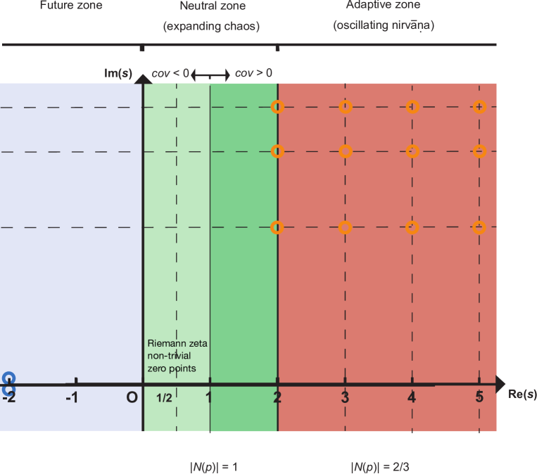
Figure 8: Visualization of an upper half-plane $\mathbb{H}$ in the PzDom model. Nontrivial zeros of the Riemann $\zeta$ function, which represent a population burst/collapse, are assumed to be at the points where the $\Re(s)=1/2$ axis intersects the horizontal broken lines (note that the scales of the horizontal and vertical axes differ). Orange circles represent adapted stages as species. The blue area represents a future stage with [$V_{p}=-\phi$, $\Re(s)\approx-1/(3\phi)$ and $\Im(s)\approx e^{-1/(3\phi)}$] [Marinõ, 2014]; converged states are indicated by blue circles. Note that $\Re(s)$ values with non-prime integers are theoretically unstable and are not observed empirically. $\Re(s)=4$ is still remarked as orange circles for ramifications, however.

It is expected that in the nirv$\overline{\mathrm{a}}$ṇa state, mutual exclusion of genetic information from different species is achieved via reproductive isolation mechanisms based on uniparental chromosome elimination [Bains and Howard, 1950] [Fujiwara et al., 1997] [Marinoni et al., 1999].

$s$ and mathematical biology

Interestingly, [Demetrius, 2006] suggests that the scaling exponents are $2/3$ for those that refer to the ratios of the fractional changes in metabolic rates to a change in body size among opportunistic species, such as annual plants and small animals (see also [White and Seymour, 2003]), but for equilibrium species, they are unity for perennial plants and $3/4$ for large animals. These values are similar to the values found for $|N(p)|$ in our model, though in this model, it is assumed that Euclidean surface area rules entail a unique minimal scaling exponent related to energy transduction localized in biomembranes. In our model, the objects are not metabolites related to biomembranes, and the assumption is not required; however, it is still possible for both models to produce metabolites with the same value. Furthermore, we showed that $a(t)\approx(M_{mass})^{|N(p)|}$. It might be interesting to survey the $|N(p)|=3/4$ case, although we note that this is considered doubtful by [Dodds et al., 2001], or to extend our study from Dictyostelium populations/species to lower-order hierarchies, such as individual/organic/tissue/cellular/organellar/molecular metabolisms. Hubble’s law could be a common point from which to understand the background logic of different hierarchies.

The output of the developed system is unpredictable when $T_{s}<T_{c}$; this is because the infinite volume limit of the system is not unique [Tasaki and Hara, 2015]. This might be the case for the simulated sympatric “speciation” presented by [de Aguiar et al., 2009].

Interactions of subgroups and mathematical physics

If there are two subgroups in a populations/species with frequency $X/Y$, then $w=w_{0}+BY-CX$ when $w_{0}$ is the fitness without benefit from interactions, $B$ is the benefit of $X$ from $Y$, and $C$ is the cost to $X$ from the interaction. Since $|D|^{E(\Sigma N)}$ is the most promising virtual benefit from noninteracting individuals, $w_{0}$ and $\Re(s)-1$ describe the overall fitness resulting from the interaction. $\Re(s)>1$ thus results in a cooperative world of higher fitness accompanied by speciation, and $0<\Re(s)<1$ results in a competitive world with a population burst/collapse with discrete characteristics. Ordered symbiosis might be involved in $\Re(s)>1$, and chaotic mutual exclusion might be involved in $0<\Re(s)<1$. This is also supported by the analysis of geodesics. When the $s$ value is in the condition of $\Re(s)-1<0$ for a significantly long duration that is not observed in [Adachi, 2015], it is possible for $q_{b}<0$ and the system is under highly competitive situation. For example, $|N(p)|=1/3$ with a contracting universe. Note that $q_{b}$ is the coefficient of $XY$ in [Zagier, 2000b], and the populations/species is harmed by competition. This case is similar to the Chern-Simons action $S_{CS}$ [Witten, 1989]:

$$S_{CS}=\frac{k_{CS}}{4\pi}\int_{M}\mathrm{tr}(A\wedge dA+\frac{2}{3}A\wedge A\wedge A),$$ (191)

where $k_{CS}$ is the integer level of the theory with a field strength of zero at all boundaries. $A$ can represent $X^{2},XY$, or $Y^{2}$ vectors, and the weight of the first term in the trace should be $0$ in adaptive situations when $X$ and $Y$ are dependent. It should be $+1/3$ in cooperative situations and $-1/3$ in competitive situations. Chern-Simons theory thus describes the action in the PzDom model, and the time derivative of the action is the Lagrangian of the system. Since the Lagrangian is $T_{s}\ln k$, when $k=constant$, $dS_{CS}/dt\cdot dT_{s}=T_{s}\ln kdT_{s}$, and $dS_{CS}=\frac{\ln k}{2\arg D}t^{2}$. Therefore, when $\arg D=constant$, $\int\int dS_{CS}dt=\frac{\ln k}{6\arg D}t^{3}=\frac{(\arg D)^{2}}{6}\ln kT_{s}^{3}$, and if $\arg D=\pi$, $\int\int dS_{CS}dt=\zeta(2)\ln kT_{s}^{3}\propto s_{d}=\frac{4}{3}a_{b}T_{s}^{3}$ when $U=a_{b}T^{4}$ in black-body radiation; note that populations/species tend to pass this boundary. Thus, $s_{d}$ is the volume of a non-Euclidean sphere with radius $T_{s}$ when $a_{b}=C_{c}/d_{c}$, where $C_{c}$ is the circumference and $d_{c}$ is the diameter. Also note that $1/\zeta(2)$ is the probability that two randomly selected integers are disjoint. That is, $\ln kT_{s}^{3}$ is the expected interaction scale of $\int\int dS_{CS}dt$, which is $T_{s}^{3}$ multiplied by the relative entropy.

There is another way of setting the Lagrangian on a boson:

$$L=i\bar{\psi}\dot{\psi}-\epsilon\bar{\psi}\psi=|D|^{2}(i\ln\dot{|D|}-\epsilon).$$ (192)

If $\epsilon\rightarrow 0$, $T_{s}\rightarrow|D|^{2}$ and $\dot{|D|}\rightarrow k$, which simplifies the calculation. If we consider a sum of relative entropies $\sum\ln k$, then $\ln k!\approx\ln(\sqrt{2\pi k}(\frac{k}{e})^{k})=\frac{1}{2}\ln(2\pi k)+k\ln(\frac{k}{e})$ when $k$ is large. The partial time-differential of $\sum\ln k$ is approximately:

$$\frac{1}{2}\frac{1}{k}\frac{\partial k}{\partial t}+(\ln k)\frac{\partial k}{\partial t}=(\frac{1}{2\dot{|D|}}+\ln\dot{|D|})\ddot{|D|}.$$ (193)

The Hamiltonian $H_{H}$ utilizes a reflectionless potential and from discrete quantum mechanics, pure imaginary shifts [Odake and Sasaki, 2015]:

$$\lim_{\gamma\rightarrow 0}\gamma^{-2}H_{H}=p_{m}^{2}-\frac{h_{H}(h_{H}+1)}{\cosh^{2}\Im(s)/b},$$ (194)

where $h_{H}=-s$. Note that $i\Im(s)/b=i\pi/2(\mathrm{mod}i\pi)$ has regular singularities.

Weights and dimensions

Interestingly, if we set a $p$-adic field $\mathbb{F}$ of $p$ other than $2$ or $3$, then the necessary and sufficient condition for root $3$ to exist in $\mathbb{F}$ is that $p\equiv 1\ \mathrm{or}\ 11\ \mathrm{mod}\ 12$. Therefore, if we stick to three dimensions comprising the interactions of identical constituents, then $p\equiv 1\ \mathrm{or}\ 11\ \mathrm{mod}\ 12$ should be satisfied. This demonstrates the symmetry of the following equations. Note that the following equation was considered by Srinivasa Ramanujan (1916?) in an unpublished manuscript:

$$F(z)=q\prod_{n=1}^{\infty}(1-q^{n})^{2}(1-q^{11n})^{2}=\sum_{n=1}^{\infty}c(n)q^{n}.$$ (195)

He proposed

$$L(s,F)=(1-c(11)11^{-s})^{-1}\times\prod_{p\neq 11}(1-c(p)p^{-s}+p^{1-2s})^{-1},$$ (196)

and later, [Eichler, 1954] proved that when $E:y^{2}+y=x^{3}-x^{2}$, $L(s,E)=L(s,F)$. It is well known that

$$\Delta(z)=q\prod_{n=1}^{\infty}(1-q^{n})^{24}=\sum_{n=1}^{\infty}\tau(n)q^{n},$$ (197)

$$L(s,\Delta)=\prod_{p:prime}(1-\tau(p)p^{-s}+p^{11-2s})^{-1},$$ (198)

and ($F$, $\Delta$) corresponds to ($1$, $11$) dimensions of the term $p$. Please note that both $F(z)$ and $\Delta(z)$ represent the interaction of two identical decompositions of 12 dimensions, multiplied by $q_{R}$. Note that $E:y^{2}+y=x^{3}-x^{2}$ implies $y(y+1)=x^{2}(x-1)$, and if the time of a phenomenon proceeds from $x$ to $x-1$, the interaction decreases from interacting $x^{2}$ to noninteracting decreased $(x-1)$. However, $\mathrm{mod}\ 4$ of the equation represents $y$ as both zero and as a three-dimensional projection of the system. The solutions of the equation should be $(0,0),(0,3),(1,0),(1,3)$. Note that $y=3$ means that the left-hand side of the equation should be $3\times 4=12$ weights. This explains the time asymmetry of the system.

To expand this discussion, consider an icosahedron and quintic equation, as in [Klein, 1993]. Note that a dihedral group is a representation of two complex conjugates. An icosahedron is composed of six conjugate $n=5$ dihedral groups and ten conjugate $n=3$ dihedral groups. The quintic dimensions include three physical space dimensions, one time dimension, and a one-dimensional interaction axis. For $n=5$, the dihedral groups can be interpreted as these quintic-dimensional functions, and the six conjugates come from the two interacting functions, each of three-dimensional fluctuations. For $n=3$, the dihedral groups can be interpreted as the three-dimensional fluctuations, and the ten conjugates are the two interacting functions, each of quintic-dimensional functions. Fifteen cross lines correspond to fifteen four-groups (two conjugates), which are the four different types ($SU(2)$) of interactions between a dimension and a three-dimensional space minus one. The system of 16 weights is the first case in which the symmetry can be completely broken, which is required for the development of the system [Tachikawa and Yonekura, 2016] [Witten, 2016].

Paddelbewegung-like motion

To expand the interpretation in Figure 8, consider the $\phi$ plane with a small $s$ value on four-groups (three physical space dimensions + one time dimension). For the physical dimensions $xyz$, we can set $\phi$ and a real parameter $\rho_{P}$ with a positive constant $a$ and

$$\left\{\begin{array}[]{l}x=(a-\rho_{P}\sin\frac{1}{2}\arg\phi)\cos\arg\phi,\\ y=(a-\rho_{P}\sin\frac{1}{2}\arg\phi)\sin\arg\phi,\\ z=\rho_{P}\cos\frac{1}{2}\arg\phi.\end{array}\right.$$ (202)

A Paddelbewegung-like motion [Weyl, 1913] follows $\rho_{P}^{\prime}=(-1)^{n_{\phi}}\rho_{P}$, $\phi^{\prime}=\phi+2n_{\phi}\pi i$, where $n_{\phi}\sim N(T)$ and $2n_{\phi}\pi\sim\Im(s)$. For a torus, consider a radius $r$ and a distance to a point from the center $R$. Addition of a real parameter $\sigma_{P}$ would lead to

$$\left\{\begin{array}[]{l}x=(R+r\cos\sigma_{P})\cos\arg\phi,\\ y=(R+r\cos\sigma_{P})\sin\arg\phi,\\ z=r\sin\sigma_{P}.\end{array}\right.$$ (206)

If we consider $\phi,\sigma_{P}$ as functions of $t$, $\frac{d\phi}{dt}\&\frac{d\sigma_{P}}{dt}$ as continuous, and $(\frac{d\phi}{dt})^{2}+(\frac{d\sigma_{P}}{dt})^{2}\neq 0$, the area of the surface $A_{\phi\sigma}$ would be

$$(\frac{dA_{\phi\sigma_{P}}}{dt})^{2}=(R+r\cos\sigma_{P})^{2}(\frac{d\phi}{dt})^{2}+r^{2}(\frac{d\sigma_{P}}{dt})^{2},$$ (207)

$\psi$ would be

$$\psi=\int_{0}^{\sigma_{P}}\frac{d\sigma_{P}}{\frac{R}{r}+\cos\sigma_{P}},$$ (208)

and $dA_{\phi\sigma_{P}}^{2}=(R+r\cos\sigma_{P})^{2}(d\phi^{2}+d\psi^{2})$. A point of a four group $(\phi,\psi)$ can be described as a translation group:

$$\left\{\begin{array}[]{l}\phi^{\prime}=\phi+2n_{\phi}\pi i\sim\phi+\Im(s)i,\\ \psi^{\prime}=\psi+\frac{2\pi r}{\sqrt{R^{2}-r^{2}}}n_{\psi}\sim\psi+\frac{2\pi}{2\pi}n_{\psi}\sim\psi+n_{\psi},\\ \end{array}\right.$$ (211)

where $\sin\theta_{\psi}=\frac{r}{R}$ as $\tan\theta_{\psi}=\frac{n_{\phi}}{T}\sim\frac{1}{2\pi}$ ($\tan\theta_{\psi}$ is a $T$-normalized quantized number $n_{\phi}$). Thus, $s$ and $w$ approximately localize at and jump among positions of integer when $\Re(s)>2$, as in orange circles of Figure 8.

Dynamical system hierarchy

Here we move to some more miscellaneous parts associated with eliminating fluctuations. Regarding the utilization of hyperbolic geometry (logarithmic-adic space) and blowing up for resolution of singularity, see our earlier work [Adachi, 2017]. From generalized function theories, the idea of cohomology naturally emerges and if we set operator III in terms of cohomology, the $H^{p}=0(p\geq 1)$ ($p$ are primes and 1) cohomology and the Kawamata-Viehweg vanishing theorem are fulfilled. This clearly demonstrates that investment in adaptation in the higher order hierarchies diminishes chaotic behavior in the hierarchies. This is because our complex manifold is a Stein manifold ($s$ is a Schwartz distribution). Furthermore, an empirical process is already introduced as “Paddelbewegung”, inspired by Hermann Weyl’s work. Other possible developments for this work include utilizing a Riemann scheme and hypergeometric differential equations or Painlevé VI equations for the hierarchical time-developing model. Consideration of an array of model types would plausibly allow exploration in relation to Galois theory and étale cohomology to interpret the hierarchical structures of natural systems, especially in biological contexts. This thus represents fruitful terrain for future research.

Finally, adopting the Atiyah-Singer index theorem, a twisted (fractal) property, Euler number of $\int_{B}e(TB)$ is obviously equal to its topological Euler characteristic, $\chi(B)=\sum(-1)^{l}l$. Hence, the analytical index of Euler class (Poincaré dual) should be the same. For evaluation of agreement, the Chern class should be $(-1)^{l}l$. On the other hand, analytically, the Hirzebruch signature (characteristic from species) of $B$ is $(-1)^{n}\int_{B}\prod_{i=1}^{n}\frac{p_{i}}{\tanh p_{i}}$, where $\frac{p_{i}}{\tanh p_{i}}=\sum_{k\geq 0}\frac{2^{2k}B_{2k}}{(2k)!}p_{i}^{2k}$. Topologically, this is equivalent to the L genus.

We are thus able to extend the methodology for the “small $s$” metric to characterize dynamical system hierarchy (adaptation and contributions) and interactions, using only abundance data along time development.

Comparison between our model and mathematical ideas

As per [Mochizuki, 2020d], a species is roughly a collection of set-theoretic formulas that gives rise to a category in any given model of set theory. For example, we can define them as a $k$-set of a single dimension $N_{k}$ with a certain topology, or a set of $(p,l,v)$ with particular morphisms. This paper completes our integrated model of species dynamics. Various interpretations according to alternative mathematical theorems are as follows.

If $\varnothing\neq\partial B$, then the Poisson-Jensen formula is applicable to $D=e^{s/b}$ and

$$\Re(s)=-b\sum_{i=1}^{n}\ln\left.|\frac{\rho^{2}-\bar{a}_{i}z}{\rho(z-a_{i})}\right.|+\frac{1}{2\pi}\int_{0}^{2\pi}\Re\left.(\frac{\rho e^{i\theta}+z}{\rho e^{i\theta}-z}\right.)\rho d\theta,$$ (212)

where $a_{i}$ is a zero point of $w=D$. The first term should be the contributions from the discrete part of $\Re(s)$ depending on the zero points of $w$ (observation phenomena) and the second term should be that from the continuous part of $\Re(s)$ ($0\leq\Re(s)<2$).

In another expression, we can regard this equation as a unique Lebesgue decomposition in the Radon-Nikodym theorem:

$$\Phi(E)=F(E)+\Psi(E),$$ (213)

where $s\in E$, a set function $\Phi(E)$ has a sigma additivity on $B$, a set function $F(E)$ has an absolute continuity, and a set function $\Psi(E)$ has singulars. Since $F(E)=\Im(s)$, $\Psi(E)=\Re(s)$, and they are expressed by the Riemann-Hurwitz formula, $\Phi(E)$ can uniquely determine the decomposition of contributions from the same hierarchy of interest $(F(E))$ and other hierarchies above $(\Psi(E))$. For another expression, universal coefficient theorems [Bott and Tu, 1982] show (a) the homology of $B$ with an abelian group of a $B$-module $G$,

$$H_{q}(B;G)\cong H_{q}(B)\otimes G\oplus\mathrm{Tor}(H_{q-1}(B),G),$$ (214)

where the first term is exactly $\Im(s)$ and the second term is $\Re(s)$; (b) the cohomology of $B$ with an abelian group of a $B$-module $G$,

$$H^{q}(B;G)\cong\mathrm{Hom}(H_{q}(B),G)\oplus\mathrm{Ext}(H_{q-1}(B),G),$$ (215)

where the first term is exactly $\Im(s)$ and the second term is $\Re(s)$. Note that, by Hodge’s theorem, the cohomology is isomorphic to harmonic oscillators in the sense that the numbers of dimensions of the former and the latter are equivalent. The cohomological dimension thus represents the number of harmonic oscillators underlying in the system of interest.

All of these mathematical formulas have interpretive value in terms of particular aspects of renormalization or fractals acting on multilevel layers and, as in biology, multilevel selections. We emphasize the potential of divergent terms as acting on higher-order hierarchies such as fractals.

Our model and statistical mechanics

In this study, we present new metrics $T_{c}$, $W$, and $S$ for distinguishing between populations and species, based simply on knowledge of the total number of individuals. We thus demonstrated spontaneous symmetry breaking of a biological system. $S$ describes the extent of ordering based on domination. The metrics presented here can also successfully evaluate the critical point $T_{c}$ and the Weiss field $W$. They can distinguish between different ordering states, such as a random distribution, a dominant species, or a population; their potential phase transitions; and adaptations ($T_{s}\approx W$). The $T_{s}\approx W$ case represents a biological application of Bose-Einstein condensation to population dynamics [Tasaki and Hara, 2015]. The theory of similar condensation phenomena was described by [Knebel et al., 2015]; besides the case in that paper, we are able to describe quantization with a case that is not a typical Bose-Einstein condensation. This is shown in Figure 3. The phase separation depends on the levels of biological hierarchies, such as a population and a species, and we can evaluate the adaptive structures allowed during the evolution in each phase: for a population-dominant phase, a single population could dominate a community; for a species-dominant phase, not a population but a sum of a given species in a community could dominate. The increasing phases correspond to the introduction of the next domination phase. Additionally, we cannot be sure of the output of a chaotic phase.

The model also shows that some highly adapted species are more stable than others. Furthermore, the zero points of the Riemann zeta function correspond to the adaptive species and also to prime numbers. The entropy $\ln k$, which was introduced in this manuscript, can be approximated by $\pi(k)/k\approx 1/\ln k$, where $\pi(k)$ is the prime counting function. The decrease in the prime number density along with the growth of entropy means that the tendency to decrease is only broken when higher-order hierarchies exist. Thus, for these organisms, higher-order hierarchies may serve as investments in adaptive ordering structures.

Now, let us consider biological hierarchies resulting from genes, cells, multicellular individuals, populations, and species. For genes and cells, if we restrict the surrounding environments to a small scale, such as cells or individuals, the copy numbers of genes and cells are nearly static, and they are no longer adaptive. Thus, $T_{s}\sim 0$ for these cases. The individuals surrounded by populations or the populations themselves are chaotic when $T_{s}\neq 0$. Our data suggest that the species level is more adaptive than are the lower-order hierarchies. For example, in Figure 3, dark blue shading indicates a population dominant phase for species dynamics as a whole, because in this regard, the entire population can be considered to be a species world; light blue, dark green, and light green indicate phases of populational chaos. We thus conclude that reproductive scales are chaotic, and to achieve adaptation, we need higher-order hierarchies. Lower-order hierarchies have the most adaptive situations, and we must extend observation from lower to higher environmental scales, such as species, communities, or ecosystems, to detect the selection pressures on genes or cells.

3.1 $s$’s relation to entropy

Regarding Landauer’s principle (e.g. [Palazzo, 2018]), $N_{k}=a-b\ln k$ means a decrease of information as $b\ln k$ from an original amount of information, $a$, in each $k$-th group. This is the central of our assumption and many aspects are drawn from this principle. For example, we adopt a partition function $\zeta(s)$ (Riemann zeta function) as an extension from Zipf’s law. In this sense, non-trivial zeros of the zeta functions become the adapted situation with diverging fitness. Thus, the inverse of fitness landscape the zeta function relates to a free energy landscape of hierarchy (e.g. [Annila and Kuismanen, 2009]) regarding its diverging nature, while $\Re(s)$ becomes a factor sublimates to the upper level and $\Im(s)$ becomes a factor restricted to the lower level. This is what proposed in [Grmela et al., 2013], as “the macroscopic systems in their reaction to imposed external forces follow some kind of optimization strategy in which their internal structure is changed so that they offer the least possible resistance”. The optimization would be natural selections of fitness in our biological model, and the potential for optimization would be the parameter small $s$, instead of entropy or entropy production in the entropy model.

$s$ as an informtaion criterion

The small $s$ value is similar to WAIC [Watanabe, 2010] in the following regards. WAIC is

$$W_{n}=T_{n}+\frac{\beta}{n}V_{n},$$ (216)

where $T_{n}$ is a training loss, $V_{n}$ is a functional variance and $\beta$ is an inverse temperature. If we use a covariance instead of $V_{n}$, $\Delta z_{k}\ln D_{k}$ becomes similar to WAIC of $k$. Therefore, $s$ is a derivative form of an information criterion of maximum likelihood estimation.

PzDom model

When $\Re(s)-1>0$, either the cooperative situation $q_{b}>0$ with $\Re(s)<2$ holds or $q_{b}=0$ with $\Re(s)>2$ without any interpopulational interaction seems to be achieved. Thus, the status of the $\Re(s)$ world is roughly separated into three cases: (i) chaotic: $0<\Re(s)<1$ with mutual exclusion; (ii) ordered: $1<\Re(s)\leq 2$ with cooperation/speciation; and (iii) most adaptively ordered: $\Re(s)>2$ with stability and no interaction (oscillating “nirv$\overline{\mathrm{a}}$ṇa” state). According to Fermat’s last theorem, the noninteracting mode of subpopulations with $q_{b}=0$ is only achieved when $X^{n}+Y^{n}=Z^{n}$ with $n\leq 2$. It is predicted that there is a possible noninteracting mode in which only a second-order nirv$\overline{\mathrm{a}}$ṇa state is continuously observed. Note that the nirv$\overline{\mathrm{a}}$ṇa state is regarded as the state of the most dominant species, and it is for a particular set of species at a particular time; it is not regarded as a fixed state for any particular species. It is also notable that when the environment is stable, the nirv$\overline{\mathrm{a}}$ṇa state is also stable. However, when the environment changes significantly, species from the previous nirv$\overline{\mathrm{a}}$ṇa state will fall into a chaotic state, rendering interactions involving competition, cooperation, and starvation-induced sexual reproduction with others. Therefore, outside of a nirv$\overline{\mathrm{a}}$ṇa state, a species must interact with other species. Furthermore, co-evolving communities in different niches cannot be described by this model, and this is a limitation of our study. It is notable that for a given niche, a noninteracting nirv$\overline{\mathrm{a}}$ṇa state is the one most likely to be dominated by a species. Consider now the Euler-Mascheroni constant:

$$\lim_{s\rightarrow 1}(\zeta(s)-\frac{1}{s-1})=\gamma=0.577....$$ (217)

When $k=1$, $|\zeta(s)|=E(\Sigma N)/N_{1}$, and in a population, it is $0.5$. Therefore, $w<0$, and in the long run, the population decreases. In a species, when $N_{1}<<E(\Sigma N)$ in a speciation phase, $w>0$. Even when $N_{1}\approx E(\Sigma N)$, $w>0$, and investing in a higher-order hierarchy of species from a populational hierarchy escapes the limit of the decreasing trend in mere populations. These species are overall adapted. The discussion here is summarized in Figure 8.

Conclusions

Only by three assumptions proposed, i.e. (1) logarithmic approximation of populations densities, (2) an exponential nature of fitness, (3) Price equation, we have successfully applied the Price equation, the $R=T$ theorem, and Weil’s explicit formula to an ecological model, which we refer to as the PzDom model, and which is based on a new topological parameter, small $s$. Species could be defined as a $p$-Sylow subgroup of a community in the single niche. The border between adaptive species and chaotic populations/species was found to be $\Re(s)=2$ (also proven by fractal theory), and the values of the norm of prime closed geodesics are $|N(p)|=2/3$ and $|N(p)|=1$, respectively. Note that mod 4 of $p$ reveals the adaptive/disadaptive situations and the Bose-Einstein condensates. The future adaptation/disadaptation of individuals is partially predictable by the Hurwitz zeta function, and we also found a time-dependent fitness function. Furthermore, we showed that it is a natural consequence of species adaptations, when considered as primes, or population conversions, when considered as geodesics, to observe a phenotypic discontinuity when maximizing information entropy. The model is able to prove the existence of biological phases of populations and species. The phases can be used to distinguish and predict different types of population and species, based on the population/species dynamics/distribution. Only by the information of population density and species classification, we can obtain this type of a partially dynamic model for future prediction without extrapolating anything. This provides a ground map for future studies to increase our understanding of the nature of hierarchical systems.

We also carefully examined the topological nature of the system and for testing purposes, species density data for a wild Dictyostelia community data are used in conjunction with data derived from liquid-chromatography mass spectrometry of proteins. Utilizing a Clifford algebra, a congruent zeta function, and a Weierstraß $\wp$ function in conjunction with a type VI Painlevé equation, we confirmed the induction of hierarchy and time through one-dimensional probability space with certain topologies. This process also served to provide information concerning interactions in the model. The previously developed “small $s$” metric can characterize dynamical system hierarchy and interactions, using only abundance data along time development.

For further clarification of induced fractals including the relation to renormalization in physics, a theoretical development is proposed based on a newly identified fact, namely that scaling parameters for magnetization exactly correspond to imaginary parts of Riemann zeta nontrivial zeros. An analogy to magnetization and accompanying Fake Monster Algebra is invoked to lend support to this theory, along with empirical species density data for a wild Dictyostelia community. A master torus and a Lagrangian/Hamiltonian are derived expressing fractal structures as a solution for diminishing divergent terms in renormalization.

4 Methods and Materials

4.1 Field Research

The data for the number of individuals in each population and species were obtained from natural (nonlaboratory) environments. The sampling method is described in [Adachi, 2015]. Field experiments were approved by the Ministry of the Environment (Japan), Ministry of Agriculture, Forestry and Fisheries (Japan), Shizuoka Prefecture (Japan) and Washidu Shrine (Japan). The approval Nos. are 23Ikan24, 24Ikan72-32, and 24Ikan72-57.

Soil samples were obtained from two point quadrats of the Washidu region of Izu in Japan. The number of individual cellular slime molds per gram of soil was determined by counting the number of plaques cultivated from soil samples. Species were identified by both morphology and by the DNA sequences of the 18S rRNA genes. Samples were obtained in each month from May 2012 to January 2013 inclusive. Calculations were performed using Microsoft Excel 12.3.6, wxMaxima 15.04.0, SageMath 8.8, R 3.3.2 and GNU Octave 3.8.0.

In more detail, sampling occurred at two $100\ \mathrm{m^{2}}$ quadrats in Washidu ($35^{\circ}3^{\prime}33^{\prime\prime}$N, $138^{\circ}53^{\prime}46^{\prime\prime}$E; $35^{\circ}3^{\prime}45^{\prime\prime}$N, $138^{\circ}53^{\prime}32^{\prime\prime}$E). Within each $100\ \mathrm{m^{2}}$ quadrat, nine sample points were established at 5 m intervals. From each sampling point, 25 g of soil was collected. Cellular slime molds were isolated from these samples as follows. First, one sample from each site was added to 25 ml of sterile water, resuspended, and then filtrated with sterile gauze. Next, $100\ \mu$l of each sample solution was mixed with $100\ \mu$l of HL5 culture medium containing Klebsiella aerogenes and spread on KK2 agar. After two days of storage in an incubator at $22\ ^{\circ}$C, the number of plaques on each agar plate was recorded. Note that the number of plaques corresponds to the total number of living cells at any possible stage of the life cycle. That is, the niche considered here is the set of propagable individuals of Dictyostelia; these are not arranged in any hierarchy or by stage in the life cycle. Also, note that we did not examine the age or size structure of organisms, since most of these were unicellular microbes. Mature fruiting bodies, consisting of the cells from a single species, were collected along with information regarding the numbers of plaques in the regions in which each fruiting body was found. Finally, spores were used to inoculate either KK2 for purification or SM/5 for expansion. All analyses were performed within two weeks from the time of collection. The isolated species were identified based on 18S rRNA (SSU) sequences, which were amplified and sequenced using PCR/sequencing primers, as described in [Medlin et al., 1988] and the SILVA database (http://www.arb-silva.de/). The recipes for the media are described at http://dictybase.org/techniques/media/media.html.

4.2 Experiments

A human HEK-293 cell line from an embryonic kidney was purchased from RIKEN (Japan). The sampling is described in [Adachi, 2017]. The original cultures were frozen on either March 18, 2013 (3-year storage) or March 5, 2014 (2-year storage). They were subsequently used in experiments between February and June 2016. The strain was cultured in Modified Eagle’s Medium (MEM) + 10% fatal bovine serum (FBS) + 0.1 mM nonessential amino acid (NEAA) at 37 ^∘C with 5% $\mathrm{CO_{2}}$. Subculturing was performed in 0.25% trypsin and prior to the experiment, the original cells from RIKEN were frozen following the standard protocol provided by RIKEN: in culture medium with 10% dimethyl sulfoxide (DMSO), they were cooled until reaching 4 ^∘C at $-$2 ^∘C/min, held at that temperature for 10 min, then cooled until reaching $-$30 ^∘C at $-$1 ^∘C/min in order to freeze, held at that temperature for 10 min, then cooled again until reaching $-$80 ^∘C at $-$5 ^∘C/min, and finally held at that temperature overnight. The next day, they were transferred to storage in liquid nitrogen.

The HEK-293 proteins were extracted using the standard protocol for the RIPA buffer (NACALAI TESQUE, INC., Kyoto, Japan). The sampling is described in [Adachi, 2017]. Approximately $10^{6}$ harvested cells were washed once in Krebs-Ringer-Buffer (KRB; 154 mM NaCl, 5.6 mM KCl, 5.5 mM glucose, 20.1 mM HEPES pH 7.4, 25 mM $\mathrm{NaHCO_{3}}$). They were resuspended in 30 $\mu$l of RIPA buffer, passed in and out through 21G needles for destruction, and incubated on ice for 1 h. They were then centrifuged at 10,000 g for 10 min at 4 ^∘C, followed by collection of the supernatants. The proteins were quantified using a Micro BCA Protein Assay Kit (Thermo Fisher Scientific, Waltham, U.S.A.) and further processing was performed using XL-Tryp Kit Direct Digestion (APRO SCIENCE, Naruto, Japan). The samples were solidified in acrylamide gel, washed twice in ultrapure water, then washed three times in dehydration solution, and finally dried. The samples were then processed using an In-Gel R-CAM Kit (APRO SCIENCE, Naruto, Japan). The samples were reduced for 2 h at 37 ^∘C, alkylated for 30 min at room temperature, washed five times with ultrapure water, washed twice with destaining solution, and then dried. The resultant samples were trypsinized overnight at 35 ^∘C. The next day, the dissolved digested peptides were collected by ZipTipC18 (Merck Millipore, Corp., Billerica, U.S.A.). The tips were dampened twice with acetonitrile and equilibrated twice with 0.1% trifluoroacetic acid. The peptides were collected by $\sim 20$ cycles of aspiration and dispensing, washed twice with 0.1% trifluoroacetic acid, and eluted by 0.1% trifluoroacetic acid /50% acetonitrile with aspiration and dispensing five times $\times$ three tips followed by vacuum drying. The final samples were stored at $-$20 ^∘C. Before undertaking LC/MS, they were resuspended in 0.1% formic acid, and the amounts were quantified by Pierce Quantitative Colorimetric Peptide Assay (Thermo Fisher Scientific, Waltham, U.S.A.). This protocol is published at http://dx.doi.org/10.17504/protocols.io.h4qb8vw.

LC/MS was undertaken by the Medical Research Support Center, Graduate School of Medicine, Kyoto University with a quadrupole–time-of-flight (Q-Tof) mass spectrometer TripleTOF 5600 (AB Sciex Pte., Ltd., Concord, Canada). Standard protocols were followed. The loading amount for each sample was 1 $\mu$g. We extracted the quantitative data for the unused information for identified proteins using ProteinPilot 4.5.0.0 software (AB Sciex Pte., Ltd., Concord, Canada). For further details see [Adachi, 2017].

5 Acknowledgments

I am very grateful to reviewers and colleagues for their comments and advice spanning medicine, biology, mathematics, and physics. I am grateful for the financial support from Tokushima University and Kyoto University, and I thank all the reviewers and colleagues who have provided me with useful comments and suggestions.

References

- [Adachi, 2015] Adachi S. 2015. Eastern Japanese Dictyostelia species adapt while populations exhibit neutrality. Evolutionary Biology 42:210-222. https://doi.org/10.1007/s11692-015-9312-0
- [Adachi, 2017] Adachi S. 2017. Rigid geometry solves “curse of dimensionality” effects in clustering methods: an application to omics data. PLOS ONE 12:e0179180. https://doi.org/10.1371/journal.pone.0179180
- [Ahlfors, 1979] Ahlfors LV. 1979. Complex analysis. New York, USA: McGraw-Hill Book Company.
- [Andrews et al., 1984] Andrews GE, Baxter RJ, Forrester PJ. 1984. Eight-vertex SOS model and generalized Rogers-Ramanujan-type identities. Journal of Statistical Physics 35:193-266. https://doi.org/10.1007/BF01014383
- [Annila and Kuismanen, 2009] Annila A, Kuismanen E. 2009. Natural hierarchy emerges from energy dispersal. BioSystems 95:227-233. https://doi.org/10.1016/j.biosystems.2008.10.008
- [Arnold et al., 1994] Arnold L, Matthias V, Demetrius L. 1994. Evolutionary formalism for products of positive random matrices. Annals of Applied Probability 4:859-901. http://dx.doi.org/10.1214/aoap/1177004975
- [Bains and Howard, 1950] Bains, GS, Howard HW. 1950. Haploid plants of Solanum demissum. Nature 166:795. https://doi.org/10.1038/166795a0
- [Banavar et al., 2010] Banavar JR, Maritan A, Volkov I. 2010. Applications of the principle of maximum entropy: from physics to ecology. Journal of Physics: Condensed Matter 22:063101. https://doi.org/10.1088/0953-8984/22/6/063101
- [Baxter, 1973] Baxter RJ. 1973. Eight-vertex model in lattice statistics and one-dimensional anisotropic Heisenberg model. Annals of Physics 76:1-71. https://doi.org/10.1016/0003-4916(73)90440-5
- [Benfatto and Gallavotti, 1995] Benfatto G, Gallavotti G. 2015. Renormalization group. Princeton, USA: Princeton University Press.
- [Bershtein and Shchechkin, 2015] Bershtein MA, Shchechkin AI. 2015. Bilinear equations on Painlevé functions from CFT. Communications in Mathematical Physics 339:1021-1061. https://doi.org/10.1007/s00220-015-2427-4
- [Bethe, 1931] Bethe HA. 1931. Zur Theorie der Metalle, I. Eigenwerte und Eigenfunktionen der linearen Atomkette. Zeitschrift für Physik 71:205-226. https://doi.org/10.1007/BF01341708
- [Bianconi et al., 2009] Bianconi G, Ferretti L, Franz S. 2009. Non-neutral theory of biodiversity. Europhysics Letters 87:28001. https://doi.org/10.1209/0295-5075/87/28001
- [Bobev et al., 2015] Bobev N, El-Showk S, Mazác D, Paulos MF. 2015. Bootstrapping the three-dimensional supersymmetric Ising model. Physical Review Letters 115:051601. https://doi.org/10.1103/PhysRevLett.115.051601
- [Borcherds, 1996] Borcherds RE. 1996. Automorphic forms and Lie algebra. Current Developments in Mathematics 1996:1-36. http://dx.doi.org/10.4310/CDM.1996.v1996.n1.a1
- [Borger, 2009] Borger J. 2009. Lambda-rings and the field with one element. arXiv:0906.3146v1 [math.NT]. https://arxiv.org/abs/0906.3146
- [Bott and Tu, 1982] Bott R, Tu LW. 1982. Differential forms in algebraic topology. New York, USA: Springer-Verlag.
- [Bridgeland, 2002] Bridgeland T. 2002. Flops and derived categories. Inventiones Mathematicae 147:613-632. https://doi.org/10.1007/s002220100185
- [Cahen, 1894] Cahen E. 1894. Sur la fonction de Riemann et sur des fonctions analogues. Annales Scientifiques de l’École Normale Supérieure, Serie 3 11:75-164. https://doi.org/10.24033/asens.401
- [Capitán et al., 2009] Capitán JA, Cuesta JA, Bascompte J. 2009. Statistical mechanics of ecosystem assembly. Physical Review Letters 103:168101. https://doi.org/10.1103/PhysRevLett.103.168101
- [Cardy, 1996] Cardy J. 1996. Scaling and renormalization in statistical physics. Cambridge, UK: Cambridge University Press.
- [Cramer, 1986] Cramer JG. 1986. The transactional interpretation of quantum mechanics. Reviews of Modern Physics 58:647-687. https://doi.org/10.1103/RevModPhys.58.647
- [de Aguiar et al., 2009] de Aguiar MAM, Baranger M, Baptestini EM, Kaufman L, Bar-Yam Y. 2009. Global patterns of speciation and diversity. Nature 460:384-387. https://doi.org/10.1038/nature08168
- [Deitmar, 1989] Deitmar A. 1989. The Selberg trace formula and the Ruelle zeta function for compact hyperbolics. Abhandlungen aus dem Mathematischen Seminar der Universität Hamburg 59:101-106. https://doi.org/10.1007/BF02942321
- [Deligne, 1974] Deligne P. 1974. La Conjecture de Weil. I. Publications Mathématiques de l’IHÉS 43:273-307. https://doi.org/10.1007/BF02684373
- [Deligne, 1977] Deligne P. 1977. Cohomologie Étale. Lecture Notes in Mathematics 569. Berlin, Germany: Springer-Verlag.
- [Deligne, 1980.] Deligne P. 1980. La Conjecture de Weil. II. Publications Mathématiques de l’IHÉS 52:137-252. https://doi.org/10.1007/BF02684780
- [Demetrius, 2006] Demetrius L. 2006. The origin of allometric scaling laws in biology. Journal of Theoretical Biology 243:455-467. https://doi.org/10.1016/j.jtbi.2006.05.031
- [Denjoy, 1931] Denjoy A. 1931. L’Hypothèse de Riemann sur la distribution des zéros de , reliée à la théorie des probabilites. Comptes Rendus de l’Académie des Sciences Paris 192: 656-658
- [Dewar and Porté, 2008] Dewar RC, Porté A. 2008. Statistical mechanics unifies different ecological patterns. Journal of Theoretical Biology 251:389-403. https://doi.org/10.1016/j.jtbi.2007.12.007
- [Dodds et al., 2001] Dodds PS, Rothman DH, Weitz JS. 2001. Re-examination of the “3/4-law” of metabolism. Journal of Theoretical Biology 209:9-27. https://doi.org/10.1006/jtbi.2000.2238
- [Dubrovin et al., 1992] Dubrovin BA, Novikov SP, Fomenko A. 1992. Modern geometry-methods and applications. Part I. The geometry of surfaces, transformation groups, and fields. Graduate studies in mathematics 93. 2nd ed. Berlin-Heidelberg-New York, Germany, USA: Springer-Verlag. p 118
- [Eguchi et al., 2011] Eguchi T, Ooguri H, Tachikawa Y. 2011. Notes on the K3 Surface and the Mathieu group . Experimental Mathematics 20:91-96. https://doi.org/10.1080/10586458.2011.544585
- [Eichler, 1954] Eichler M. 1954. Quaternäre quadratische Formen und die Riemannsche Vermutung für die Kongruenzzetafunktion. Archiv der Mathematik 5:355-366. https://doi.org/10.1007/BF01898377
- [Emch, 1899-1900] Emch A. 1899-1900. Illustration of the elliptic integrals of the first kind by a certain link-work. Annals of mathematics. Ser. 2 1:81-92. http://doi.org/10.2307/1967273
- [Emch, 1900-1901.] Emch A. 1900-1901. An application of elliptic functions to Peaucellier’s link-work (inversor). Annals of mathematics. Ser. 2 2:60-63. http://doi.org/10.2307/2007182
- [Fisher et al., 1943] Fisher RA, Corbet AS, Williams CB. 1943. The relation between the number of species and the number of individuals in a random sample of animal population. Journal of Animal Ecology 12:42-58. https://doi.org/10.2307/1411
- [Fujisaka, 1998] Fujisaka H. 1998. Statistical mechanics of nonequilibrium systems. Tokyo, Japan: Sangyo Tosho. In Japanese
- [Fujiwara et al., 1997] Fujiwara A, Abe S, Yamaha E, Yamazaki F, Yoshida MC. 1997. Uniparental chromosome elimination in the early embryogenesis of the inviable salmonid hybrids between mass salmon female and rainbow trout male. Chromosoma 106:44-52. https://doi.org/10.1007/s004120050223
- [Gaiotto et al., 2016] Gaiotto D, Moore GW, Witten E. 2017. An introduction to the web-based formalism. Confluentes Mathematici 9:5-48 https://doi.org/10.5802/cml.40
- [Gamayun et al., 2012] Gamayun O, Iorgov N, Lisovyy O. 2012. Conformal field theory of Painlevé VI. Journal of High Energy Physics 10:38. https://doi.org/10.1007/JHEP10(2012)038
- [Gavrylenko and Lisovyy, 2018] Gavrylenko P, Lisovyy O. 2018. Fredholm determinant and Nekrasov sum representations of isomonodromic tau functions. Communications in Mathematical Physics 363:1-58. https://doi.org/10.1007/s00220-018-3224-7
- [Grmela et al., 2013] Grmela M, Grazzini G, Lucia U, Yahia L’H. 2013. Multiscale mesoscopic entropy of driven macroscopic systems. Entropy 15:5053-5064. https://doi.org/10.3390/e15115053
- [Guckenheimer and Holmes, 1983] Guckenheimer J, Holmes P. 1983. Nonlinear oscillations, dynamical dystems, and bifurcations of vector fields. New York-Berlin-Heidelberg-Tokyo, USA-Germany-Japan: Springer-Verlag.
- [Harte et al., 2008] Harte J, Zillio T, Conlisk E, Smith AB. 2008. Maximum entropy and the state-variable approach to macroecology. Ecology 89:2700-2711. https://doi.org/10.1890/07-1369.1
- [Hartshorne, 1977] Hartshorne R. 1977. Algebraic geometry. Berlin, New York, Germany-USA: Springer-Verlag.
- [Hubbard, 2006] Hubbard JH. 2006. Teichmüller theory and applications to geometry. Topology and Dynamics, Vol. 1, Teichmüller Theory. Ithaca, USA: Matrix Editions.
- [Hubbell, 1997] Hubbell SP. 1997. A unified theory of biogeography and relative species abundance and its application to tropical rain forests and coral reefs. Coral Reefs 16:s9-s21. https://doi.org/10.1007/s003380050237
- [Hubbell, 2001] Hubbell SP. 2001. The Unified Neutral Theory of Biodiversity and Biogeography. Princeton, USA: Princeton University Press.
- [Iorgov et al., 2015] Iorgov N, Lisovyy O, Teschner J. 2015. Isomonodromic tau-functions from Liouville conformal blocks. Communications in Mathematical Physics 336:671. https://doi.org/10.1007/s00220-014-2245-0
- [Jimbo, 1996] Jimbo M, Sakai H. 1996. A -analog of the sixth Painlevé equation. Letters in Mathematical Physics 38:145-154. https://doi.org/10.1007/BF00398316
- [Juhl, 2001] Juhl A. 2001. Cohomological theory of dynamical zeta functions. Basel, Switzerland: Birkhäuser.
- [Kachru and Tripathy, 2017] Kachru S, Tripathy A. 2017. The hidden symmetry of the heterotic string. Advances in Theoretical and Mathematical Physics 21:1729-1745. https://dx.doi.org/10.4310/ATMP.2017.v21.n7.a5
- [Kakei and Kikuchi, 2007] Kakei S, Kikuchi T. 2007. The sixth Painlevé equation as similarity reduction of generalized Drinfel’d-Sokolov hierarchy. Letters in Mathematical Physics 79:221-234. https://doi.org/10.1007/s11005-007-0144-4
- [Károlyházy, 1966] Károlyházy F. 1966. Gravitation and quantum mechanics of macroscopic objects (*). Il Nuovo Cimento 52:390-402. https://doi.org/10.1007/BF02717926
- [Károlyházy et al., 1986] Károlyházy F, Frenkel A, Lukács B. 1986. On the possible role of gravity in the reduction of the wave function. In: Penrose R., Isham CJ (eds) Quantum concepts in space and time. Oxford, UK: Oxford University Press pp 109-128.
- [Kashiwara and Schapira, 2018] Kashiwara M, Schapira P. 2018. Persistent homology and microlocal sheaf theory. Journal of Applied and Computational Topology 2:83-113. https://doi.org/10.1007/s41468-018-0019-z
- [Katz, 2009] Katz NM. 2009. Twisted L-functions and monodromy. Princeton, USA: Princeton University Press.
- [Kawakami et al., 2016] Kawakami H, Nakamura A, Sakai H. 2016. Degeneration scheme of 4-dimensional Painlevé-type equations. arXiv:1209.3836v3 [math.CA]. https://arxiv.org/abs/1209.3836
- [Kedlay, 2010] Kedlaya KS. 2010. -adic differential equations. Cambridge, UK: Cambridge University press.
- [Kerner, 1957] Kerner EH. 1957. A statistical mechanics of interacting biological species. Bulletin of Mathematical Biology 19:121-146. https://doi.org/10.1007/BF02477883
- [Kimura, 1964] Kimura M. 1964. Diffusion models in population genetics. Journal of Applied Probability 1:177-232. https://doi.org/10.2307/3211856
- [Kisin, 2009] Kisin M. 2009. Moduli of finite flat group schemes, and modularity. Annals of Mathematics 170:1085-1180. https://doi.org/10.4007/annals.2009.170.1085
- [Klein, 1883] Klein F. 1883. Neue Beiträge zur Riemannschen Funktionentheorie. Mathematische Annalen 21:141-218. https://doi.org/10.1007/BF01442920
- [Klein, 1993] Klein FC. 1993. Vorlesungen über das Ikosaeder und die Auflösung der Gleichungen vom fünften Grade. Leipzig, Germany: Teubner BG.
- [Knebel et al., 2015] Knebel J, Weber MF, Krüger T, Frey E. 2015. Evolutionary games of condensates in coupled birth-death processes. Nature Communications 6:6977. https://doi.org/10.1038/ncomms7977
- [Knuth, 1997] Knuth D. 1997. The art of computer programming, 2: seminumerical algorithms. 3rd ed. Boston, USA: Addison-Wesley Professional.
- [Kobayashi and Nomizu, 1996] Kobayashi S, Nomizu K. 1996. Foundations of differential geometry, vol. 2. Hoboken, USA: Wiley-Interscience.
- [Koebe, 1907a] Koebe P. 1907a. Über die Uniformisierung reeller analytischer Kurven. Gött Nachr 1907:177-190
- [Koebe, 1907b] Koebe P, 1907b. Über die Uniformisierung beliebiger analytischer Kurven. Gött Nachr 1907:191-210
- [Koebe, 1907c] Koebe P, 1907c. Über die Uniformisierung beliebiger analytischer Kurven (Zweite Mitteilung). Gött Nachr 1907:633-669
- [Kramar et al., 2016] Kramár M, Levanger R, Tithof J, Suri B, Xu M, Paul M, et al. 2016. Analysis of Kolmogorov flow and Rayleigh-Bénard convection using persistent homology. Physica D 334:82-98. https://doi.org/10.1016/j.physd.2016.02.003
- [Kurokawa, 1987] Kurokawa N. 1987. On certain Euler products. Acta Arithmetica 48:49-52. https://doi.org/10.4064/aa-48-1-49-52
- [Lambert, 1998] Lambert ND. 1998, D-brane bound states and the generalised ADHM construction. Nuclear Physics B 519:214-224. https://doi.org/10.1016/S0550-3213(98)00026-1