Routing Autonomous Vehicles in Congested Transportation Networks: Structural Properties and Coordination Algorithms

Abstract

This paper considers the problem of routing and rebalancing a shared fleet of autonomous (i.e., self-driving) vehicles providing on-demand mobility within a capacitated transportation network, where congestion might disrupt throughput. We model the problem within a network flow framework and show that under relatively mild assumptions the rebalancing vehicles, if properly coordinated, do not lead to an increase in congestion (in stark contrast to common belief). From an algorithmic standpoint, such theoretical insight suggests that the problem of routing customers and rebalancing vehicles can be decoupled, which leads to a computationally-efficient routing and rebalancing algorithm for the autonomous vehicles. Numerical experiments and case studies corroborate our theoretical insights and show that the proposed algorithm outperforms state-of-the-art point-to-point methods by avoiding excess congestion on the road. Collectively, this paper provides a rigorous approach to the problem of congestion-aware, system-wide coordination of autonomously driving vehicles, and to the characterization of the sustainability of such robotic systems.

I Introduction

Autonomous (i.e., robotic, self-driving) vehicles are rapidly becoming a reality and hold great promise for increasing safety and enhancing mobility for those unable or unwilling to drive [1, 2]. A particularly attractive operational paradigm involves coordinating a fleet of autonomous vehicles to provide on-demand service to customers, also called autonomous mobility-on-demand (AMoD). An AMoD system may reduce the cost of travel [3] as well as provide additional sustainability benefits such as increased overall vehicle utilization, reduced demand for urban parking infrastructure, and reduced pollution (with electric vehicles) [1]. The key benefits of AMoD are realized through vehicle sharing, where each vehicle, after servicing a customer, drives itself to the location of the next customer or rebalances itself throughout the city in anticipation of future customer demand [4].

In terms of traffic congestion, however, there has been no consensus on whether autonomous vehicles in general, and AMoD systems in particular, will ultimately be beneficial or detrimental. It has been argued that by having faster reaction times, autonomous vehicles may be able to drive faster and follow other vehicles at closer distances without compromising safety, thereby effectively increasing the capacity of a road and reducing congestion. They may also be able to interact with traffic lights to reduce full stops at intersections [5]. On the downside, the process of vehicle rebalancing (empty vehicle trips) increases the total number of vehicles on the road (assuming the number of vehicles with customers stays the same). Indeed, it has been argued that the presence of many rebalancing vehicles may contribute to an increase in congestion [6, 7]. These statements, however, do not take into account that in an AMoD system the operator has control over the actions (destination and routes) of the vehicles, and may route vehicles intelligently to avoid increasing congestion or perhaps even decrease it.

Accordingly, the goal of this paper is twofold. First, on an engineering level, we aim to devise routing and rebalancing algorithms for an autonomous vehicle fleet that seek to minimize congestion. Second, on a socio-economic level, we aim to rigorously address the concern that autonomous cars may lead to increased congestion and thus disrupt currently congested transportation infrastructures.

Literature review: In this paper, we investigate the problem of controlling an AMoD system within a road network in the presence of congestion effects. Previous work on AMoD systems have primarily concentrated on the rebalancing problem [4, 3], whereby one strives to allocate empty vehicles throughout a city while minimizing fuel costs or customer wait times. The rebalancing problem has been studied in [4] using a fluidic model and in [8] using a queueing network model. An alternative formulation is the one-to-one pickup and delivery problem [9], where a fleet of vehicles service pickup and delivery requests within a given region. Combinatorial asymptotically optimal algorithms for pickup and delivery problems were presented in [10, 11], and generalized to road networks in [12]. Almost all current approaches assume point-to-point travel between origins and destinations (no road network), and even routing problems on road networks (e.g. [12]) do not take into account vehicle-to-vehicle interactions that would cause congestion and reduce system throughput.

On the other hand, traffic congestion has been studied in economics and transportation for nearly a century. The first congestion models [13, 14, 15] sought to formalize the relationship between vehicle speed, density, and flow. Since then, approaches to modeling congestion have included empirical [16], simulation-based [17, 18, 19], queueing-theoretical [20], and optimization [21, 22]. While there have been many high fidelity congestion models that can accurately predict traffic patterns, the primary goal of congestion modeling has been the analysis of traffic behavior. Efforts to control traffic have been limited to the control of intersections [23, 24] and freeway on-ramps [25] because human drivers behave non-cooperatively. The problem of cooperative, system-wide routing (a key benefit of AMoD systems) is similar to the dynamic traffic assignment problem (DTA) [22] and to [26, 27] in the case of online routing. The key difference is that these approaches only optimize routes for passenger vehicles while we seek to optimize the routes of both passenger vehicles and empty rebalancing vehicles.

Statement of contributions: The contribution of this paper is threefold. First, we model an AMoD system within a network flow framework, whereby customer-carrying and empty rebalancing vehicles are represented as flows over a capacitated road network (in such model, when the flow of vehicles along a road reaches a critical capacity value, congestion effects occur). Within this model, we provide a cut condition for the road graph that needs to be satisfied for congestion-free customer and rebalancing flows to exist. Most importantly, under the assumption of a symmetric road network, we investigate an existential result that leads to two key conclusions: (1) rebalancing does not increase congestion, and (2) for certain cost functions, the problems of finding customer and rebalancing flows can be decoupled. Second, leveraging the theoretical insights, we propose a computationally-efficient algorithm for congestion-aware routing and rebalancing of an AMoD system that is broadly applicable to time-varying, possibly asymmetric road networks. Third, through numerical studies on real-world traffic data, we validate our assumptions and show that the proposed real-time routing and rebalancing algorithm outperforms state-of-the-art point-to-point rebalancing algorithms in terms of lower customer wait times by avoiding excess congestion on the road.

Organization: The remainder of this paper is organized as follows: in Section II we present a network flow model of an AMoD system on a capacitated road network and formulate the routing and rebalancing problem. In Section III we present key structural properties of the model including fundamental limitations of performance and conditions for the existence of feasible (in particular, congestion-free) solutions. The insights from Section III are used to develop a practical real-time routing and rebalancing algorithm in Section IV. Numerical studies and simulation results are presented in Section V, and in Section VI we draw conclusions and discuss directions for future work.

II Model Description and Problem Formulation

In this section we formulate a network flow model for an AMoD system operating over a capacitated road network. The model allows us to derive key structural insights into the vehicle routing and rebalancing problem, and motivates the design of real-time, congestion-aware algorithms for coordinating the robotic vehicles. We start in Section II-A with a discussion of our congestion model; then, in Section II-B we provide a detailed description of the overall AMoD system model.

II-A Congestion Model

We use a simplified congestion model consistent with classical traffic flow theory [13]. In classical traffic flow theory, at low vehicle densities on a road link, vehicles travel at the free flow speed of the road (imposed by the speed limit). This is referred to as the free flow phase of traffic. In this phase, the free flow speed is approximately constant [28]. The flow, or flow rate, is the number of vehicles passing through the link per unit time, and is given by the product of the speed and density of vehicles. When the flow of vehicles reaches an empirically observed critical value, the flow reaches its maximum. Beyond the critical flow rate, vehicle speeds are dramatically reduced and the flow decreases, signaling the beginning of traffic congestion. The maximum stationary flow rate is called the capacity of the road link in the literature. In our approach, road capacities are modeled as constraints on the flow of vehicles. In this way, the model captures the behavior of vehicles up to the onset of congestion.

This simplified congestion model is adequate for our purposes because the goal is not to analyze the behavior of vehicles in congested networks, but to control vehicles in order to avoid the onset of congestion. We also do not explicitly model delays at intersections, spillback behavior due to congestion, or bottleneck behavior due to the reduction of the number of lanes on a road link. An extension to our model that accommodates (limited) congestion on links is presented in Section V-A.

II-B Network Flow Model of AMoD system

We consider a road network modeled as a directed graph $G=(\mathcal{V},\mathcal{E})$, where $\mathcal{V}$ denotes the node set and $\mathcal{E}\subseteq\mathcal{V}\times\mathcal{V}$ denotes the edge set. Figure 1 shows one such network. The nodes $v$ in $\mathcal{V}$ represent intersections and locations for trip origins/destinations, and the edges $(u,v)$ in $\mathcal{E}$ represent road links. As discussed in Section II-A, congestion is modeled by imposing capacity constraints on the road links: each constraint represents the capacity of the road upon the onset of congestion. Specifically, for each road link $(u,v)\in\mathcal{E}$, we denote by $c(u,v):\mathcal{E}\mapsto\mathbb{N}_{>0}$ the capacity of that link. When the flow rate on a road link is less than the capacity of the link, all vehicles are assumed to travel at the free flow speed, or the speed limit of the link. For each road link $(u,v)\in\mathcal{E}$, we denote by $t(u,v):\mathcal{E}\mapsto\mathbb{R}_{\geq 0}$ the corresponding free flow time required to traverse road link $(u,v)$. Conversely, when the flow rate on a road link is larger than the capacity of the link, the traversal time is assumed equal to $\infty$ (we reiterate that our focus in this section is on avoiding the onset of congestion).

We assume that the road network is capacity-symmetric (or symmetric for short): for any cut $(\mathcal{S},\bar{\mathcal{S}})$ of $G(\mathcal{V},\mathcal{E})$, the overall capacity of the edges connecting nodes in $\mathcal{S}$ to nodes in $\bar{\mathcal{S}}$ equals the overall capacity of the edges connecting nodes in $\bar{\mathcal{S}}$ to nodes in $\mathcal{S}$, that is

$$\sum_{(u,v)\in\mathcal{E}:\,\,u\in\mathcal{S},\,v\in\bar{S}}c(u,v)=\sum_{(v,u)\in\mathcal{E}:\,\,u\in\mathcal{S},\,v\in\bar{S}}c(v,u)$$

It is easy to verify that a network is capacity-symmetric if and only if the overall capacity entering each node equals the capacity exiting each node., i.e.

$$\sum_{u\in\mathcal{V}:(u,v)\in\mathcal{E}}c(u,v)=\sum_{w\in\mathcal{V}:(v,w)\in\mathcal{E}}c(v,w)$$

If all edges have symmetrical capacity, i.e., for all $(u,v)\in\mathcal{E}$, $c(u,v)=c(v,u)$, then the network is capacity-symmetric. The converse statement, however, is not true in general.

Transportation requests are described by the tuple $(s,t,\lambda)$, where $s\in\mathcal{V}$ is the origin of the requests, $t\in\mathcal{V}$ is the destination, and $\lambda\in\mathbb{R}_{>0}$ is the rate of requests, in customers per unit time. Transportation requests are assumed to be stationary and deterministic, i.e., the rate of requests does not change with time and is a deterministic quantity. The set of transportation requests is denoted by $\mathcal{M}=\{(s_{m},t_{m},\lambda_{m})\}_{m}$, and its cardinality is denoted by $M$.

Single-occupancy vehicles travel within the network while servicing the transportation requests. We denote $f_{m}(u,v):\mathcal{E}\mapsto\mathbb{R}_{\geq 0}$, $m=\{1,\ldots,M\}$, as the customer flow for requests $m$ on edge $(u,v)$, i.e., the amount of flow from origin $s_{m}$ to destination $t_{m}$ that uses link $(u,v)$. We also denote $f_{R}(u,v):\mathcal{E}\mapsto\mathbb{R}_{\geq 0}$ as the rebalancing flow on edge $(u,v)$, i.e., the amount of rebalancing flow traversing edge $(u,v)$ needed to realign the vehicles with the asymmetric distribution of transportation requests.

II-C The Routing Problem

The goal is to compute flows for the autonomous vehicles that (i) transfer customers to their desired destinations in minimum time (customer-carrying trips) and (ii) rebalance vehicles throughout the network to realign the vehicle fleet with transportation demand (customer-empty trips). Specifically, the Congestion-free Routing and Rebalancing Problem (CRRP) is formally defined as follows. Given a capacitated, symmetric network $G(\mathcal{V},\mathcal{E})$, a set of transportation requests $\mathcal{M}=\{(s_{m},t_{m},\lambda_{m})\}_{m}$, and a weight factor $\rho>0$, solve

$$\!\!\!\!\underset{f_{m}(\cdot,\cdot),f_{R}(\cdot,\cdot)}{\text{minimize}} \!\!\!\!\!\!\!\sum_{m\in\mathcal{M}}\sum_{(u,v)\in\mathcal{E}}t(u,v)f_{m}(u,v)\!+\!\rho\sum_{(u,v)\in\mathcal{E}}t(u,v)f_{R}(u,v)$$ (1)

subject to $$\!\!\!\!\!\!\!\!\sum_{u\in\mathcal{V}}f_{m}(u,s_{m})+\lambda_{m}=\sum_{w\in\mathcal{V}}f_{m}(s_{m},w)\;\;\forall m\in\mathcal{M}$$ (2)

$$\!\!\!\!\!\!\!\!\sum_{u\in\mathcal{V}}f_{m}(u,t_{m})=\lambda_{m}+\sum_{w\in\mathcal{V}}f_{m}(t_{m},w)\;\;\forall m\in\mathcal{M}$$ (3)

$$\!\!\!\!\!\!\!\!\sum_{u\in\mathcal{V}}f_{m}(u,v)=\sum_{w\in\mathcal{V}}f_{m}(v,w)$$

$$\!\!\!\!\!\!\!\!\qquad\qquad\qquad\qquad\forall m\in\mathcal{M},v\in\mathcal{V}\setminus\{s_{m},t_{m}\}$$ (4)

$$\!\!\!\!\!\!\!\!\sum_{u\in\mathcal{V}}f_{R}(u,v)+\sum_{m\in\mathcal{M}}1_{v=t_{m}}\lambda_{m}$$

$$\!\!\!\!\!\!\!\!=\sum_{w\in\mathcal{V}}f_{R}(v,w)+\sum_{m\in\mathcal{M}}1_{v=s_{m}}\lambda_{m}\quad\forall v\in\mathcal{V}$$ (5)

$$\!\!\!\!\!\!\!\!f_{R}(u,v)+\sum_{m\in\mathcal{M}}f_{m}(u,v)\leq c(u,v)\;\;\forall(u,v)\in\mathcal{E}$$ (6)

Figure 1: A road network modeling Lower Manhattan and the Financial District. Nodes (denoted by small black dots) model intersections; select nodes, denoted by colored circular and square markers, model passenger trips’ origins and destinations. Different trip requests are denoted by different colors. Roads are modeled as edges; line thickness is proportional to road capacity.

The cost function (1) is a weighted sum (with weight $\rho$) of the overall duration of all passenger trips and the duration of rebalancing trips. Constraints (2), (3) and (4) enforce continuity of each trip (i.e., flow conservation) across nodes. Constraint (5) ensures that vehicles are rebalanced throughout the road network to re-align vehicle distribution with transportation requests, i.e. to ensure that every outbound customer flow is matched by an inbound flow of rebalancing vehicles and vice versa. Finally, constraint (6) enforces the capacity constraint on each link (function $1_{x}$ denotes the indicator function of the Boolean variable $x=\{\text{true, false}\}$, that is $1_{x}$ equals one if $x$ is true, and equals zero if $x$ is false). Note that the CRRP is a linear program and, in particular, a special instance of the fractional multi-commodity flow problem [29].

We denote a customer flow $\{f_{m}(u,v)\}_{(u,v),m}$ that satisfies Equations (2), (3), (4) and (6) as a feasible customer flow. For a given set of feasible customer flows $\{f_{m}(u,v)\}_{(u,v),m}$, we denote a flow $\{f_{R}(u,v)\}_{(u,v)}$ that satisfies Equation (5) and such that the combined flows $\{f_{m}(u,v),f_{R}(u,v)\}_{(u,v),m}$ satisfy Equation (6) as a feasible rebalancing flow. We remark that a rebalancing flow that is feasible with respect to a set of customer flows may be infeasible for a different collection of customer flows.

For a given set of optimal flows $\{f_{m}^{*}(u,v)\}_{(u,v),m}$ and $\{f_{R}^{*}(u,v)\}_{(u,v)}$, the minimum number of vehicles needed to implement them is given by

$$V_{\text{min}}=\left\lceil\sum_{m\in\mathcal{M}}\sum_{(u,v)\in\mathcal{E}}t(u,v)\Big{(}f_{m}^{*}(u,v)+f_{R}^{*}(u,v)\Big{)}\right\rceil.$$

This follows from a similar analysis done in [4] for point-to-point networks. Hence, the cost function (1) is aligned with the desire of minimizing the number of vehicles needed to operate an AMoD system.

II-D Discussion

A few comments are in order. First, we assume that transportation requests are time invariant. This assumption is valid when transportation requests change slowly with respect to the average duration of a customer’s trip, which is often the case in dense urban environments [30]. Additionally, in Section IV we will present algorithmic tools that allow one to extend the insights gained from the time-invariant case to the time-varying counterpart. Second, the assumption of single-occupancy for the vehicles models most of the existing (human) one-way vehicle sharing systems (where the driver is considered “part” of the vehicle), and chiefly disallows the provision of ride-sharing or carpooling service (this is an aspect left for future research). Third, as also discussed in Section II-A, our congestion model is simpler and less accurate than typical congestion models used in the transportation community. However, our model lends itself to efficient real-time optimization and thus it is well-suited to the control of fleets of autonomous vehicles. Existing high-fidelity congestion models should be regarded as complementary and could be used offline to identify the congestion thresholds used in our model. Fourth, while we have defined the CRRP in terms of fractional flows, an integer-valued counterpart can be defined and (approximately) solved to find optimal routes for each individual customer and vehicle. Algorithmic aspects will be investigated in depth in Section IV, with the goal of devising practical, real-time routing and rebalancing algorithms. Fifth, trip requests are assumed to be known. In practice, trip requests can be reserved in advance, estimated from historical data, or estimated in real time. Finally, the assumption of capacity-symmetric road networks indeed appears reasonable for a number of major U.S. metropolitan areas (note that this assumption is much less restrictive than assuming every individual road is capacity-symmetric). In the Supplementary Material, by using OpenStreetMap data [31], we provide a rigorous characterization in terms of capacity symmetry of the road networks of New York City, Chicago, Los Angeles and other major U.S. cities. The results consistently show that urban road networks are usually symmetric to a very high degree. Additionally, several of our theoretical and algorithmic results extend to the case where this assumption is lifted, as it will be highlighted throughout the paper.

III Structural Properties of the
Network Flow Model

In this section we provide two key structural results for the network flow model presented in Section II-B. First, we provide a cut condition that needs to be satisfied for feasible customer and rebalancing flows to exist. In other words, this condition provides a fundamental limitation of performance for congestion-free AMoD service in a given road network. Second, we investigate an existential result (our main theoretical result) that is germane to two key conclusions: (1) rebalancing does not increase congestion in symmetric road networks, and (2) for certain cost functions, the problems of finding customer and rebalancing flows can be decoupled – an insight that will be heavily exploited in subsequent sections.

III-A Fundamental Limitations

We start with a few definitions. For a given set of feasible customer flows $\{f_{m}(u,v)\}_{(u,v),m}$, we denote by $F_{\text{out}}(\mathcal{S},\bar{\mathcal{S}})$ the overall flow exiting a cut $(\mathcal{S},\bar{\mathcal{S}})$, i.e., $F_{\text{out}}(\mathcal{S},\bar{\mathcal{S}}):=\sum_{m\in\mathcal{M}}\sum_{u\in\mathcal{S},v\in\bar{\mathcal{S}}}f_{m}(u,v)$. Similarly, we denote by $C_{\text{out}}(\mathcal{S},\bar{\mathcal{S}})$ the capacity of the network exiting $\mathcal{S}$, i.e., $C_{\text{out}}(\mathcal{S},\bar{\mathcal{S}})=\sum_{u\in S,v\in\bar{\mathcal{S}}}c(u,v)$. Analogously, $F_{\text{in}}(\mathcal{S},\bar{\mathcal{S}})$ denotes the overall flow entering $\mathcal{S}$ from $\bar{\mathcal{S}}$, i.e., $F_{\text{in}}(\mathcal{S},\bar{\mathcal{S}}):=F_{\text{out}}(\bar{\mathcal{S}},\mathcal{S})$, and $C_{\text{in}}(\mathcal{S},\bar{\mathcal{S}})$ denotes the capacity entering $\mathcal{S}$ from $\bar{\mathcal{S}}$, i.e., $C_{\text{in}}(\mathcal{S},\bar{\mathcal{S}}):=C_{\text{out}}(\bar{\mathcal{S}},{\mathcal{S}})$. We highlight that the arguments leading to the main result of this subsection (Theorem III.4) do not require the assumption of capacity symmetry; hence, Theorem III.4 holds for asymmetric road networks as well.

The next technical lemma (whose proof is provided in the Supplementary Material) shows that the net flow leaving set $\mathcal{S}$ equals the difference between the flow originating from the origins $s_{m}$ in $\mathcal{S}$ and the flow exiting through the destinations $t_{m}$ in $\mathcal{S}$, that is,

Lemma III.1 (Net flow across a cut)

Consider a set of feasible customer flows $\{f_{m}(u,v)\}_{(u,v),m}$. Then, for every cut $(\mathcal{S},\bar{\mathcal{S}})$, the net flow leaving set $\mathcal{S}$ satisfies

$$F_{\text{out}}(\mathcal{S},\bar{\mathcal{S}})-F_{\text{in}}(\mathcal{S},\bar{\mathcal{S}})=\sum_{m\in\mathcal{M}}1_{s_{m}\in\mathcal{S}}\lambda_{m}-\sum_{m\in\mathcal{M}}1_{t_{m}\in\mathcal{S}}\lambda_{m}.$$

We now state two additional lemmas (whose proofs are given in the Supplementary Material) providing, respectively, lower and upper bounds for the outflows $F_{\text{out}}(\mathcal{S},\bar{\mathcal{S}})$.

Lemma III.2 (Lower bound for outflow)

Consider a set of feasible customer flows $\{f_{m}(u,v)\}_{(u,v),m}$. Then, for any cut $(\mathcal{S},\bar{\mathcal{S}})$, the overall flow $F_{\text{out}}(\mathcal{S},\bar{\mathcal{S}})$ exiting cut $(\mathcal{S},\bar{\mathcal{S}})$ is lower bounded according to

$$\sum_{m\in\mathcal{M}}1_{s_{m}\in\mathcal{S},t_{m}\in\bar{\mathcal{S}}}\lambda_{m}\leq F_{\text{out}}(\mathcal{S},\bar{\mathcal{S}}).$$

Lemma III.3 (Upper bound for outflow)

Assume there exists a set of feasible customer and rebalancing flows $\{f_{m}(u,v),\,f_{R}(u,v)\}_{(u,v),m}$. Then, for every cut $(\mathcal{S},\bar{\mathcal{S}})$,

1. $F_{\text{out}}(\mathcal{S},\bar{\mathcal{S}})\leq C_{\text{out}}(\mathcal{S},\bar{\mathcal{S}})$, and

2. $F_{\text{out}}(\mathcal{S},\bar{\mathcal{S}})\leq C_{\text{in}}(\mathcal{S},\bar{\mathcal{S}})$.

We are now in a position to present a structural (i.e., flow-independent) necessary condition for the existence of feasible customer and rebalancing flows.

Theorem III.4 (Necessary condition for feasible flows)

A necessary condition for the existence of a set of feasible customer and rebalancing flows $\{f_{m}(u,v),\,f_{R}(u,v)\}_{(u,v),m}$, is that, for every cut $(\mathcal{S},\bar{\mathcal{S}})$,

1. $\sum_{m\in\mathcal{M}}1_{s_{m}\in\mathcal{S},t_{m}\in\bar{\mathcal{S}}}\lambda_{m}\leq C_{\text{out}}(\mathcal{S},\bar{\mathcal{S}})$, and

2. $\sum_{m\in\mathcal{M}}1_{s_{m}\in\mathcal{S},t_{m}\in\bar{\mathcal{S}}}\lambda_{m}\leq C_{\text{in}}(\mathcal{S},\bar{\mathcal{S}})$.

Proof:

The theorem is a trivial consequence of Lemmas III.2 and III.3. ∎

Theorem III.4 essentially provides a structural fundamental limitation of performance for a given road network: if the cut conditions in Theorem III.4 are not met, then there is no hope of finding congestion-free customer and rebalancing flows. We reiterate that Theorem III.4 holds for both symmetric and asymmetric networks (for a symmetric network, claim 2) in Lemma III.3 and condition 2) in Theorem III.4 are redundant).

III-B Existence of Congestion-Free Flows

In this section we address the following question: assuming there exists a feasible customer flow, is it always possible to find a feasible rebalancing flow? As we will see, the answer to this question is affirmative and has both conceptual and algorithmic implications.

Theorem III.5 (Feasible rebalancing)

Assume there exists a set of feasible customer flows $\{f_{m}(u,v)\}_{(u,v),m}$. Then, it is always possible to find a set of feasible rebalancing flows $\{f_{R}(u,v)\}_{(u,v)}$.

Proof:

We prove the theorem for the special case where no node $v\in\mathcal{V}$ is associated with both an origin and a destination for the transportation requests in $\mathcal{M}$. This is without loss of generality, as the general case where a node $v$ has both an origin and a destination assigned can be reduced to this special case, by associating with node $v$ a “shadow” node so that (i) all destinations are assigned to the shadow node and (ii) node $v$ and its shadow node are mutually connected via an infinite-capacity, zero-travel-time edge.

We start the proof by defining the concepts of partial rebalancing flows and defective origins and destinations. Specifically, a partial rebalancing flow, denoted as $\{\hat{f}_{R}(u,v)\}_{(u,v)}$, is a set of mappings from $\mathcal{E}$ to _≥0 obeying the following properties:

1. It satisfies constraint (5) at every node that is not an origin nor a destination, that is $\forall\,v\in\{\mathcal{V}\setminus\{\{s_{m}\}_{m}\cup\{t_{m}\}_{m}\}\}$,

   $$\sum_{u\in\mathcal{V}}\hat{f}_{R}(u,v)=\sum_{w\in\mathcal{V}}\hat{f}_{R}(v,w).$$

2. It violates constraint (5) in the “$\leq$ direction” at every node that is an origin, that is $\forall\,v\in\mathcal{V}\text{ such that }\,\exists m\in\mathcal{M}:v=s_{m}$,

   $$\sum_{u\in\mathcal{V}}\hat{f}_{R}(u,v)\leq\sum_{w\in\mathcal{V}}\hat{f}_{R}(v,w)+\sum_{m\in\mathcal{M}}1_{v=s_{m}}\lambda_{m}.$$

3. It violates constraint (5) in the “$\geq$ direction” at every node that is a destination, that is $\forall\,v\in\mathcal{V}\text{ such that }\,\exists m\in\mathcal{M}:v=t_{m}$,

   $$\sum_{u\in\mathcal{V}}\hat{f}_{R}(u,v)+\sum_{m\in\mathcal{M}}1_{v=t_{m}}\lambda_{m}\geq\sum_{w\in\mathcal{V}}\hat{f}_{R}(v,w).$$

4. The combined customer and partial rebalancing flows $\{f_{m}(u,v),\hat{f}_{R}(u,v)\}_{(u,v),m}$ satisfy Equation (6) for every edge $(u,v)\in\mathcal{E}$.

Note that the trivial zero flow, that is $\hat{f}_{R}(u,v)=0$ for all $(u,v)\in\mathcal{E}$, is a partial rebalancing flow (in other words, the set of partial rebalancing flows in not empty). Clearly a feasible rebalancing flow is also a partial rebalancing flow, but the opposite is not necessarily true.

For a given partial rebalancing flow, we denote an origin node, that is a node $v\in\mathcal{V}$ such that $v=s_{m}$ for some $m=1,\ldots,M$, as a defective origin if Equation (5) is not satisfied at $v=s_{m}$ (in other words, the strict inequality $<$ holds). Analogously, we denote a destination node, that is a node $v\in\mathcal{V}$ such that $v=t_{m}$ for some $m=1,\ldots,M$, as a defective destination if Equation (5) is not satisfied at $v=t_{m}$ (in other words, the strict inequality $>$ holds). The next lemma (whose proof is provided in the Supplementary Material) links the concepts of partial rebalancing flows and defective origins/destinations.

Lemma III.6 (Co-existence of defective origins/destinations)

For every partial rebalancing flow that is not a feasible rebalancing flow, there exists at least one node $u\in\mathcal{V}$ that is a defective origin, and one node $v\in\mathcal{V}$ that is a defective destination.

For a given set of customer flows $\{f_{m}(u,v)\}_{(u,v),m}$ and partial rebalancing flows $\{\hat{f}_{R}(u,v)\}_{(u,v)}$, we call an edge $(u,v)\in\mathcal{E}$ saturated if Equation (6) holds with equality for that edge. We call a path saturated if at least one of the edges along the path is saturated. We now prove the existence of a special partial rebalancing flow where defective destinations and defective origins are separated by a graph cut formed exclusively by saturated edges (this result, and its consequences, are illustrated in Figure 2).

Lemma III.7

Assume there exists a set of feasible customer flows $\{f_{m}(u,v)\}_{(u,v),m}$, but there does not exist a set of feasible rebalancing flows $\{f_{R}(u,v)\}_{(u,v)}$. Then, there exists a partial rebalancing flow $\{\hat{f}_{R}(u,v)\}_{(u,v)}$ that induces a graph cut $(\mathcal{S},\bar{\mathcal{S}})$ with the following properties: (i) all defective destinations are in $\mathcal{S}$, (ii) all defective origins are in $\bar{\mathcal{S}}$, and (iii) all edges in $(S,\bar{\mathcal{S}})$ are saturated.

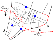
Figure 2: A graphical representation of Lemma III.7. If there exists a set of feasible customer flows but there does not exist a set of feasible rebalancing flows, one can find a partial rebalancing flow where all the defective origins, represented as blue circles, are separated from all the defective destinations, represented as blue squares, by a cut of saturated edges (shown in red). Note that not all saturated edges necessarily belong to the cut. In the proof of Theorem III.5 we show that the capacity of such a cut $(\mathcal{S},\bar{\mathcal{S}})$ is asymmetric, i.e., $C_{\text{out}}<C_{\text{in}}$ – a contradiction that leads to the claim of Theorem III.5.

We are now in a position to prove Theorem III.5. The proof is by contradiction. Assume that a set of feasible rebalancing flows $\{f_{R}(u,v)\}_{(u,v)}$ does not exist. Then Lemma III.7 shows that there exists a partial rebalancing flow $\{\hat{f}_{R}(u,v)\}_{(u,v)}$ and a cut ($\mathcal{S},\bar{\mathcal{S}}$) such that all defective destinations under $\{\hat{f}_{R}(u,v)\}_{(u,v)}$ belong to $\mathcal{S}$ and all defective origins belong to $\bar{\mathcal{S}}$. Let us denote the sum of all partial rebalancing flows across cut $(\mathcal{S},\bar{\mathcal{S}})$ as

$$\hat{F}^{\text{reb}}_{\text{out}}(\mathcal{S},\bar{\mathcal{S}}):=\sum_{u\in\mathcal{S},v\in\bar{\mathcal{S}}}\hat{f}_{R}(u,v),$$

and, analogously, define $\hat{F}^{\text{reb}}_{\text{in}}(\mathcal{S},\bar{\mathcal{S}}):=\hat{F}^{\text{reb}}_{\text{out}}(\bar{\mathcal{S}},\mathcal{S})$. Since all edges in the cut $(\mathcal{S},\bar{\mathcal{S}})$ are saturated under $\{\hat{f}_{R}(u,v)\}_{(u,v)}$, one has, due to Equation (6), the equality

$$C_{\text{out}}(\mathcal{S},\bar{\mathcal{S}})=F_{\text{out}}(\mathcal{S},\bar{\mathcal{S}})+\hat{F}^{\text{reb}}_{\text{out}}(\mathcal{S},\bar{\mathcal{S}}).$$

Additionally, again due to Equation (6), one has the inequality

$$F_{\text{in}}(\mathcal{S},\bar{\mathcal{S}})+\hat{F}^{\text{reb}}_{\text{in}}(\mathcal{S},\bar{\mathcal{S}})\leq C_{\text{in}}(\mathcal{S},\bar{\mathcal{S}}).$$

Combining the above equations, one obtains

$$F_{\text{in}}(S,\bar{S})+\hat{F}^{\text{reb}}_{\text{in}}(\mathcal{S},\bar{\mathcal{S}})-F_{\text{out}}(\mathcal{S},\bar{\mathcal{S}})-\hat{F}^{\text{reb}}_{\text{out}}(\mathcal{S},\bar{\mathcal{S}})\leq C_{\text{in}}(\mathcal{S},\bar{\mathcal{S}})-C_{\text{out}}(\mathcal{S},\bar{\mathcal{S}}).$$

To compute $\hat{F}^{\text{reb}}_{\text{in}}(\mathcal{S},\bar{\mathcal{S}})-\hat{F}^{\text{reb}}_{\text{out}}(\mathcal{S},\bar{\mathcal{S}})$, we follow a procedure similar to the one used in Lemma III.1. Summing Equation (5) over all nodes in $\mathcal{S}$, one obtains,

$$\sum_{v\in\mathcal{S}}\left[\sum_{u\in\mathcal{V}}\hat{f}_{R}(u,v)+\sum_{m\in\mathcal{M}}1_{v=t_{m}}\lambda_{m}\right]$$

$$\qquad\qquad>\sum_{v\in\mathcal{S}}\left[\sum_{w\in\mathcal{V}}\hat{f}_{R}(v,w)+\sum_{m\in\mathcal{M}}1_{v=s_{m}}\lambda_{m}\right].$$

The strict inequality is due to the fact that for a partial rebalancing flow that is not feasible there exists at least one defective destination (Lemma III.6), which, by construction, must belong to $\mathcal{S}$. Simplifying those flows $\hat{f}_{R}(u,v)$ for which both $u$ and $v$ are in $\mathcal{S}$ (as such flows appear on both sides of the above inequality), one obtains

$$\hat{F}^{\text{reb}}_{\text{in}}(\mathcal{S},\bar{\mathcal{S}})-\hat{F}^{\text{reb}}_{\text{out}}(\mathcal{S},\bar{\mathcal{S}})> \sum_{m\in\mathcal{M}}1_{s_{m}\in\mathcal{S}}\lambda_{m}-\sum_{m\in\mathcal{M}}1_{t_{m}\in\mathcal{S}}\lambda_{m}.$$

Also, by Lemma III.1,

$$F_{\text{out}}(\mathcal{S},\bar{\mathcal{S}})-F_{\text{in}}(\mathcal{S},\bar{\mathcal{S}})=\sum_{m\in\mathcal{M}}1_{s_{m}\in\mathcal{S}}\lambda_{m}-\sum_{m\in\mathcal{M}}1_{t_{m}\in\mathcal{S}}\lambda_{m}.$$

Collecting all the results so far, we conclude that

$$0 <F_{\text{in}}(S,\bar{S})+\hat{F}^{\text{reb}}_{\text{in}}(\mathcal{S},\bar{\mathcal{S}})-F_{\text{out}}(\mathcal{S},\bar{\mathcal{S}})-\hat{F}^{\text{reb}}_{\text{out}}(\mathcal{S},\bar{\mathcal{S}})$$

$$=C_{\text{in}}(\mathcal{S},\bar{\mathcal{S}})-C_{\text{out}}(\mathcal{S},\bar{\mathcal{S}}).$$

Hence, we reached the conclusion that $C_{\text{in}}(\mathcal{S},\bar{\mathcal{S}})-C_{\text{out}}(\mathcal{S},\bar{\mathcal{S}})>0$, or, in other words, the capacity of graph $G(\mathcal{V},\mathcal{E})$ across cut $(\mathcal{S},\bar{\mathcal{S}})$ is not symmetric. This contradicts the assumption that graph $G(\mathcal{V},\mathcal{E})$ is capacity-symmetric, and the claim follows. ∎

The importance of Theorem III.5 is twofold. First, perhaps surprisingly, it shows that for symmetric road networks it is always possible to rebalance the autonomous vehicles without increasing congestion – in other words, the rebalancing of autonomous vehicles in a symmetric road network does not lead to an increase in congestion. Second, from an algorithmic standpoint, if the cost function in the CRRP only depends on the customer flows (that is, $\rho=0$ and the goal is to minimize the customers’ travel times), then the CRRP problem can be decoupled and the customers and rebalancing flows can be solved separately without loss of optimality. This insight will be instrumental in Section IV to the design of real-time algorithms for routing and rebalancing.

We conclude this section by noticing that the CRRP, from a computational standpoint, can be reduced to an instance of the Minimum-Cost Multi-Commodity Flow problem (Min-MCF), a classic problem in network flow theory [29]. The problem can be efficiently solved either via linear programming (the size of the linear program is $|\mathcal{E}|(M+1)$), or via specialized combinatorial algorithms [32, 33, 34]. However, the solution to the CRRP provides static fractional flows, which are not directly implementable for the operation of actual AMoD systems. Practical algorithms (inspired by the theoretical CRRP model) are presented in the next section.

IV Real-time Congestion-Aware
Routing and Rebalancing

A natural approach to routing and rebalancing would be to periodically resolve the CRRP within a receding-horizon, batch-processing scheme (a common scheme for the control of transportation networks [35, 4, 36]). This approach, however, is not directly implementable as the solution to the CRRP provides fractional flows (as opposed to routes for the individual vehicles). This shortcoming can be addressed by considering an integral version of the CRRP (dubbed integral CRRP), whereby the flows are integer-valued and can be thus easily translated into routes for the individual vehicles, e.g. through a flow decomposition algorithm [37]. The integral CRRP, however, is an instance of the integral Minimum-Cost Multi-Commodity Flow problem, which is known to be NP-hard [38, 39]. Naïve rounding techniques are inapplicable: rounding a solution for the (non-integral) CRRP does not yield, in general, feasible integral flows, and hence feasible routes. For example, continuity of vehicles and customers can not be guaranteed, and vehicles may appear and disappear along a route. In general, to the best of our knowledge, there are no polynomial-time approximation schemes for the integral Minimum-Cost Multi-Commodity Flow problem.

On the positive side, the integral CRRP admits a decoupling result akin to Theorem III.5: given a set of feasible, integral customer flows, one can always find a set of feasible, integral rebalancing flows. (In fact, the proof of Theorem III.5 does not exploit anywhere the property that the flows are fractional, and thus the proof extends virtually unchanged to the case where the flows are integer-valued). Our approach is to leverage this insight (and more in general the theoretical results from Section III) to design a heuristic, yet efficient approximation to the integral CRRP that (i) scales to large-scale systems, and (ii) is general, in the sense that can be broadly applied to time-varying, asymmetric networks.

Specifically, we consider as objective the minimization of the customers’ travel times, which, from Section III and the aforementioned discussion about the generalization of Theorem III.5 to integral flows, suggests that customer routing can be decoupled from vehicle rebalancing (strictly speaking, this statement is only valid for static and symmetric networks – its generalization beyond these assumptions will be addressed numerically in Section V). Accordingly, to emulate the real-world operation of an AMoD system, we divide a given city into geographic regions (also referred to as “stations” in some formulations) [4, 8], and each arriving customer is assigned the closest vehicle within that region (vehicle imbalance across regions is handled separately by the vehicle rebalancing algorithm, discussed below). We apply a greedy, yet computationally-efficient and congestion-aware approach for customer routing where customers are routed to their destinations using the shortest-time path as computed by an $A^{*}$ algorithm [40]. The travel time along each edge is computed using a heuristic delay function that is related to the current volume of traffic on each edge. In this work, for each edge $(u,v)\in\mathcal{E}$ we use the simple Bureau of Public Roads (BPR) delay model [41]

$$t_{d}(u,v):=t(u,v)\left(1+\alpha\left(\frac{f(u,v)}{c(u,v)}\right)^{\beta}\right),$$

where $f(u,v):=\sum_{m=1}^{M}\,f_{m}(u,v)+f_{R}(u,v)$ is the total flow on edge $(u,v)$, and $\alpha$ and $\beta$ are usually set to $0.15$ and $4$ respectively. Note that customer routing is event-based, i.e, a routing choice is made as soon as a customer arrives.

Separately from customer routing, vehicle rebalancing from one region to another is performed every $t_{\text{hor}}>0$ time units as a batch process (unlike customer routing, which is an event-based process). Denote by $v_{i}(t)$ the number of vehicles in region $i$ at time $t$, and by $v_{ji}(t)$ the number of vehicles traveling from region $j$ to $i$ that will arrive in the next $t_{\text{vicinity}}$ time units. Let $v^{\text{own}}_{i}(t):=v_{i}(t)+\sum_{j}v_{ji}(t)$ be the number of vehicles currently “owned” by region $i$ (i.e., in the vicinity of such region). Denote by $v^{e}_{i}(t)$ the number of excess vehicles in region $i$, or the number of vehicles left after servicing the customers waiting within region $i$. From its definition, $v^{e}_{i}(t)$ is given by $v^{e}_{i}(t)=v^{\text{own}}_{i}(t)-c_{i}(t)$, where $c_{i}(t)$ is the number of customers within region $i$. Finally, denote by $v^{d}_{i}(t)$ the desired number of vehicles within region $i$. For example, for an even distribution of excess vehicles, $v^{d}_{i}(t)\propto\sum_{i}v^{e}_{i}(t)/N$, where $N$ is the number regions. Note that the $v^{d}_{i}(t)$’s are rounded so they take on integer values. The set of origin regions (i.e., regions that should send out vehicles), $S_{R}$, and destination regions (i.e., regions that should receive vehicles), $T_{R}$, for the rebalancing vehicles are then determined by comparing $v^{e}_{i}(t)$ and $v^{d}_{i}(t)$, specifically,

$$\text{if }v^{e}_{i}(t) >v^{d}_{i}(t),\;\;\;\;\text{region }i\in S_{R}$$

$$\text{if }v^{e}_{i}(t) <v^{d}_{i}(t),\;\;\;\;\text{region }i\in T_{R}.$$

We assume the residual capacity $c_{R}(u,v)$ of an edge $(u,v)$, defined as the difference between its overall capacity $c(u,v)$ and the current number of vehicles along that edge, is known and remains approximately constant over the rebalancing time horizon. In case the overall rebalancing problem is not feasible (i.e. it is not possible to move all excess vehicles to regions that have a deficit of vehicles while satisfying the congestion constraints), we define slack variables with cost $C$ that allow the optimizer to select a subset of vehicles and rebalancing routes of maximum cardinality such that each link does not become congested. The slack variables are denoted as $ds_{i}$ for each $i\in S_{R}$, and $dt_{j}$ for each $j\in T_{R}$.

Every $t_{\text{hor}}$ time units, the rebalancing vehicle routes are computed by solving the following integer linear program

$$\underset{f_{R}(\cdot,\cdot),\{ds_{i}\},\{dt_{j}\}}{\text{minimize}} \!\!\sum_{(u,v)\in\mathcal{E}}t(u,v)\,f_{R}(u,v)\ +\sum_{i\in S_{R}}Cds_{i}+\sum_{i\in T_{R}}Cdt_{i}$$

subject to $$\sum_{u\in\mathcal{V}}f_{R}(u,v)+1_{v\in S_{R}}(v^{e}_{v}(t)-v^{d}_{v}(t)-ds_{v})$$

$$=\sum_{w\in V}f_{R}(v,w)+1_{v\in T_{R}}(v^{d}_{v}(t)-v^{e}_{v}(t)-dt_{v}),$$

$$\qquad\qquad\qquad\qquad\qquad\qquad\qquad\text{for all }v\in\mathcal{V}$$

$$f_{R}(u,v)\leq c_{R}(u,v),\;\;\;\;\text{for all }(u,v)\in\mathcal{E}$$

$$f_{R}(u,v)\in\mathbb{N},\qquad\text{for all }(u,v)\in\mathcal{E}$$

$$ds_{i},dt_{j}\in\mathbb{N},\qquad\text{for all }i\in S_{R},j\in T_{R}$$

The set of (integral) rebalancing flows $\{f_{R}(u,v)\}_{(u,v)}$ is then decomposed into a set of rebalancing paths via a flow decomposition algorithm [37]. Each rebalancing path connects one origin region with one destination region: thus, rebalancing paths represent the set of routes that excess vehicles should follow to rebalance to regions with a deficit of vehicles.

The rebalancing optimization problem is an instance of the Minimum Cost Flow problem. If all edge capacities are integral, the linear relaxation of the Minimum Cost Flow problem enjoys a totally unimodular constraint matrix [29]. Hence, the linear relaxation will necessarily have an integer optimal solution, which will be a fortiori an optimal solution to the original Minimum Cost Flow problem. It follows that an integer-valued solution to the rebalancing optimization problem can be computed efficiently, namely in polynomial time, e.g., via linear programming. Several efficient combinatorial algorithms [29] are also available, whose computational performance is typically significantly better.

The favorable computational properties of the routing and rebalancing algorithm presented in this section enable application to large-scale systems, as described next.

V Numerical Experiments

In this section, we characterize the effect of rebalancing on congestion in asymmetric network and explore the performance of the algorithm presented in Section IV on real-world road topologies with real customer demands.

V-A Characterization of Congestion due to Rebalancing in Asymmetric Networks

The theoretical results in Section III are proven for capacity-symmetric networks, which are in general a reasonable model for typical urban road networks (we refer the reader to the Supplementary Material for a detailed analysis of capacity symmetry for major U.S. cities). Nevertheless, it is of interest to characterize the applicability of our theoretical results (chiefly, the existential result in Theorem III.5) to road networks that significantly violate the capacity-symmetry property. In other words, we study to what degree rebalancing might lead to an increase in congestion if the network is asymmetric.

To this purpose, we compute solutions to the CRRP for road networks with varying degrees of capacity asymmetry and we compare corresponding travel times to those obtained by computing optimal routes in the absence of rebalancing (as it would be the case, e.g., if the vehicles were privately owned). We focus on the road network portrayed in Figure 3, which captures all major streets and avenues in Manhattan. Transportation requests are based on actual taxi rides in New York City on March 1, 2012 from 6 to 8 p.m. (courtesy of the New York Taxi and Limousine Commission). We randomly selected about one third of the trips that occurred in that time frame (roughly 17,000 trips) and we adjusted the capacities of the roads such that the flows induced by these trips would approach the threshold of congestion. The roads considered all have similar speed limits and comparable number of lanes and thus we assign to each edge in the network the same capacity, specifically, one vehicle every 23.6 seconds. This capacity is consistent with the observations that (i) the customer flow is only $30\%$ of the real one (so road capacity is reduced accordingly) and (ii) taxis only contribute to a fraction of the overall traffic in Manhattan. Nevertheless, we stress that the capacity was selected specifically to ensure that the flow induced by the trips would approach the threshold of congestion before any asymmetry is induced. To investigate the effects of network asymmetry, we introduce an artificial capacity asymmetry into the baseline Manhattan road network by progressively reducing the capacity of all northbound avenues.

In order to gain a quantitative understanding of the effect of rebalancing on congestion and travel times, we introduce slack variables $\delta_{C}(u,v)$, associated with a cost $c_{c}(u,v)$, to each congestion constraint (6). The cost $c_{c}(u,v)$ is selected so that the optimization algorithm will select a congestion-free solution whenever one is available. Once a solution is found, the actual travel time on each (possibly congested) link is computed with the heuristic BPR delay model [41] presented in Section IV. This approach maintains feasibility even in the congested traffic regime, and hence allows us to assess the impact of rebalancing on congestion in asymmetric networks.

Figure 3 summarizes the results of our simulations. In the baseline case, no artificial capacity asymmetry is introduced, i.e., the fractional capacity reduction of northbound avenues is equal to 0%. In this case, the customer routing problem with no rebalancing (essentially, the CRRP problem with the rebalancing flows constrained to be equal to zero) admits a congestion-free solution. On the other hand, the CRRP requires a (very small) relaxation of the congestion constraints. Overall, the difference between the travel times in the two cases is very small and approximately equal to 2.12%, in line with the fact that New York City’s road graph has largely symmetric capacity, as discussed in Section II and shown in the Supplementary Material. Interestingly, even with a massive $50\%$ reduction in northbound capacity, travel times when rebalancing vehicles are present are within $4.12\%$ of those obtained assuming no rebalancing is performed. Collectively, these results show that the existential result in Theorem III.5, proven under the assumption of a symmetric network, appears to extend (even though approximately) to asymmetric networks. In particular, it appears that vehicle rebalancing does not lead to an appreciable increase in congestion under very general conditions.

We conclude this section by noticing that for a $40\%$ reduction in capacity, the travel times with vehicle rebalancing dip slightly lower than those without. This effect is due to our use of the BPR link delay model: while in our theoretical model the time required to traverse a link is constant so long as a link is uncongested, the link delay in the BPR model varies by as much as $15\%$ between free-flow and the onset of congestion.

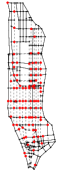
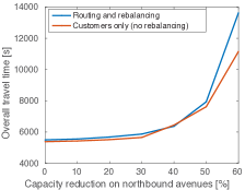
Figure 3: Left: Manhattan road network. One-way roads are represented as dashed lines. Centers of rebalancing regions are represented in red. Right: Customer travel times with and without rebalancing for different levels of network asymmetry.

V-B Congestion-Aware Real-time Rebalancing

In this section we evaluate the performance of the real-time routing and rebalancing algorithm presented in Section IV against a baseline approach that does not explicitly take congestion into account. We simulate $7,000$ vehicles providing service to actual taxi requests on March 1, 2012, for two hours between 6 and 8 p.m., using the same Manhattan road network as in the previous section (see Figure 3). Taxi requests are clustered into 88 regions corresponding to a subset of nodes in the road network. Road capacities are reduced to account for exogenous vehicles on the roads to the point that congestion occurs along some routes during the simulation. The free flow speed of the vehicles is set to 25 mph (11 m/s) and approximately 55,000 trip requests (from the taxi data set discussed before) are simulated using a time step of 6 seconds. The simulated speed of the vehicles on each link depend on the number of vehicles in the link, and is calculated using the BPR model. Other delay factors such as traffic signals, turning times, and pedestrian blocking are not simulated.

Three simulations are performed, namely (i) assuming every customer has access to a private vehicle with no rebalancing, (ii) using the congestion-aware routing and rebalancing algorithm presented in Section IV, and (iii) using a baseline rebalancing algorithm. The baseline approach is derived from the real-time rebalancing algorithm presented in [8], which is a point-to-point algorithm that computes rebalancing origins and destinations without considering the underlying road network. In the baseline approach, customer routes are computed in the same way as in Section IV. For rebalancing, the origins and destinations are first solved using the algorithm provided in [8], then the routes are computed using the $A^{*}$ algorithm much like the customer routes. In simulations (ii) and (iii), rebalancing is performed every 2 minutes.

Table I presents a summary of the performance results for simulations (ii) and (iii). Note that the service time is the total time a customer spends in the system (waiting $+$ traveling).

TABLE I: Results of the real-time simulations

Performance metric	Congestion-aware	Baseline
# of trips completed	49,585	42,219
mean wait time (all trips)	163.57 s	406.03 s
mean travel time (completed trips)	265.13 s	275.19 s
mean service time (completed trips)	286.96 s	324 s
% with wait time $>$ 5 minutes	5.4%	20%
mean # of rebalancing vehicles	204	1489

Only data from simulations (ii) and (iii) are presented in Table I because the only applicable performance metric in simulation (i) is the mean travel time which was 264.69 s. Comparing our algorithm with (i), we notice that the additional rebalancing vehicles have no significant impact on the travel time. Comparing our algorithm with (iii), we notice that the congestion-aware algorithm outperforms the baseline algorithm in every metric: low congestion allows the vehicles to service customers faster, resulting in a reduction in wait times as well as travel times. The baseline algorithm will send rebalancing vehicles to stations with a deficit of vehicles regardless of the level of congestion in the road network. This results in many more empty vehicles dispatched to rebalance the system (see Table I), which causes heavy congestion in the network. Our congestion-aware algorithm drastically reduces this effect, resulting in very few congested road links.

VI Conclusions and Future Work

In this paper we presented a network flow model of an autonomous mobility-on-demand system on a capacitated road network. We formulated the routing and rebalancing problem and showed that on symmetric road networks, it is always possible to route rebalancing vehicles in a coordinated way that does not increase traffic congestion. Using a model road network of Manhattan, we showed that rebalancing did not increase congestion even for moderate degrees of network asymmetry. We leveraged the theoretical insights to develop a computationally efficient real-time congestion-aware routing and rebalancing algorithm and demonstrated its performance over state-of-the-art point-to-point rebalancing algorithms through simulation. This highlighted the importance of congestion awareness in the design and implementation of control strategies for a fleet of self-driving vehicles.

This work opens the field to many future avenues of research. First, note that the solution to the integral CRRP can directly be used as a practical routing algorithm. For large scale systems, high-quality approximate solutions for the integral CRRP may be obtained using randomized algorithms [42, 43]. Second, from a modeling perspective, we would like to study the inclusion of stochastic information (e.g., demand prediction, travel time uncertainty) for the routing and rebalancing problem, as well as a richer set of performance metrics and constraints (e.g., time windows to pick up customers). Third, it is worthwhile to study how our results give intuition into business models for autonomous urban mobility (e.g. fleet sizes). Fourth, it is of interest to explore other approaches that may reduce congestion, including ride-sharing, demand staggering, and integration with public transit to create an intermodal transportation network. Fifth, we would like to explore decentralized architectures for cooperative routing and rebalancing. Finally, we would like to demonstrate the real-world performance of the algorithms using high fidelity microscopic traffic simulators and by implementing them on real fleets of self-driving vehicles.

Supplementary Material:
Proofs of Technical Results

Proof:

We compute the sum over all customer flows $m\in\mathcal{M}$ and over all nodes $v\in\mathcal{V}$ of the node balance equation for flow $m$ at node $v$ (Equation (3) if node $v$ is the source of $m$, Equation (4) if node $v$ is the sink of $m$, or Equation (2) otherwise). We obtain

$$\sum_{v\in\mathcal{S}}\sum_{m\in\mathcal{M}} \left(\sum_{u\in\mathcal{V}}f_{m}(u,v)+1_{v=s_{m}}\lambda_{m}\right)=$$

$$\sum_{v\in\mathcal{S}}\sum_{m\in\mathcal{M}}\left(\sum_{w\in\mathcal{V}}f_{m}(v,w)+1_{v=t_{m}}\lambda_{m}\right).$$

For any edge $(u,v)$ such that $u,v\in\mathcal{S}$, the customer flow $f_{m}(u,v)$ appears on both sides of the equation. Thus the equation above simplifies to

$$\sum_{m\in\mathcal{M}}\sum_{v\in\mathcal{S}} \left(\sum_{u\in\bar{\mathcal{S}}}f_{m}(u,v)+1_{v=s_{m}}\lambda_{m}\right)=$$

$$\sum_{m\in\mathcal{M}}\sum_{v\in\mathcal{S}}\left(\sum_{w\in\bar{\mathcal{S}}}f_{m}(v,w)+1_{v=t_{m}}\lambda_{m}\right),$$

which leads to the claim of the lemma

$$F_{\text{in}}(\mathcal{S},\bar{\mathcal{S}})+\sum_{m\in\mathcal{M}}1_{s_{m}\in\mathcal{S}}\lambda_{m}=F_{\text{out}}(\mathcal{S},\bar{\mathcal{S}})+\sum_{m\in\mathcal{M}}1_{t_{m}\in\mathcal{S}}\lambda_{m}.$$

∎

Proof:

Adding Equations (2), (3) and (4) over all nodes in $\mathcal{S}$ and over all flows whose origin is in $\mathcal{S}$ and whose destination is in $\bar{\mathcal{S}}$, one obtains

$$\sum_{m:s_{m}\in\mathcal{S},t_{m}\in\bar{\mathcal{S}}}\,\,\sum_{v\in\mathcal{S}} \left(\sum_{u\in\mathcal{V}}f_{m}(u,v)+1_{v=s_{m}}\lambda_{m}\right)=$$

$$\sum_{m:s_{m}\in\mathcal{S},t_{m}\in\bar{\mathcal{S}}}\sum_{v\in\mathcal{S}}\left(\sum_{w\in\mathcal{V}}f_{m}(v,w)\right).$$

Flows $f_{m}(u,v)$ such that both $u$ and $v$ are in $\mathcal{S}$ appear on both sides of the equation. Simplifying, one obtains

$$\sum_{m:s_{m}\in\mathcal{S},t_{m}\in\bar{\mathcal{S}}}\lambda_{m}=$$

$$\sum_{m:s_{m}\in\mathcal{S},t_{m}\in\bar{\mathcal{S}}}\left(\sum_{v\in\mathcal{S},w\in\bar{\mathcal{S}}}f_{m}(v,w)-\sum_{v\in\mathcal{S},u\in\bar{\mathcal{S}}}f_{m}(u,v)\right)$$

The first term on the right-hand side represents a lower bound for $F_{\text{out}}(\mathcal{S},\bar{\mathcal{S}})$, since

$$F_{\text{out}}(\mathcal{S},\bar{\mathcal{S}})= \sum_{m\in\mathcal{M}}\sum_{v\in\mathcal{S},w\in\bar{\mathcal{S}}}f_{m}(v,w)$$

$$\geq \sum_{m:s_{m}\in\mathcal{S},t_{m}\in\bar{\mathcal{S}}}\sum_{v\in\mathcal{S},w\in\bar{\mathcal{S}}}f_{m}(v,w).$$

Furthermore, the second term on the right-hand side is upper-bounded by zero. The lemma follows. ∎

Proof:

The first condition follows trivially from equation (6). As for the second condition, consider a cut $(\mathcal{S},\bar{\mathcal{S}})$. Analogously as for the definitions of $F_{\text{in}}(\mathcal{S},\bar{\mathcal{S}})$ and $F_{\text{out}}(\mathcal{S},\bar{\mathcal{S}})$, let $F^{\text{reb}}_{\text{in}}(\mathcal{S},\bar{\mathcal{S}})$ and $F^{\text{reb}}_{\text{out}}(\mathcal{S},\bar{\mathcal{S}})$ denote, respectively, the overall rebalancing flow entering (exiting) cut $(\mathcal{S},\bar{\mathcal{S}})$. Summing equation (5) over all nodes in $S$, one easily obtains

$$F^{\text{reb}}_{\text{in}}(\mathcal{S},\bar{\mathcal{S}})-F^{\text{reb}}_{\text{out}}(\mathcal{S},\bar{\mathcal{S}})=\sum_{m\in\mathcal{M}}1_{s_{m}\in\mathcal{S}}\lambda_{m}-\sum_{m\in\mathcal{M}}1_{t_{m}\in\mathcal{S}}\lambda_{m}.$$

Combining the above equation with Lemma III.1, one obtains

$$F^{\text{reb}}_{\text{in}}(\mathcal{S},\bar{\mathcal{S}})-F^{\text{reb}}_{\text{out}}(\mathcal{S},\bar{\mathcal{S}})=F_{\text{out}}(\mathcal{S},\bar{\mathcal{S}})-F_{\text{in}}(\mathcal{S},\bar{\mathcal{S}}),$$

in other words, rebalancing flows should make up the difference between the customer inflows and outflows across cut $(\mathcal{S},\bar{\mathcal{S}})$. Accordingly, the total inflow of vehicles across $(\mathcal{S},\bar{\mathcal{S}})$, $F^{\text{tot}}_{\text{in}}(\mathcal{S},\bar{\mathcal{S}})$, satisfies the inequality

$$F^{\text{tot}}_{\text{in}}(\mathcal{S},\bar{\mathcal{S}}): =F_{\text{in}}(\mathcal{S},\bar{\mathcal{S}})+F^{\text{reb}}_{\text{in}}(\mathcal{S},\bar{\mathcal{S}})$$

$$=F_{\text{in}}(\mathcal{S},\bar{\mathcal{S}})+F^{\text{reb}}_{\text{out}}(\mathcal{S},\bar{\mathcal{S}})+F_{\text{out}}(\mathcal{S},\bar{\mathcal{S}})-F_{\text{in}}(\mathcal{S},\bar{\mathcal{S}})$$

$$\geq F_{\text{out}}(\mathcal{S},\bar{\mathcal{S}}).$$

Since the customer and rebalancing flows $\{f_{m}(u,v),\,f_{R}(u,v)\}_{(u,v),m}$ are feasible, then, by equation (6), $F^{\text{tot}}_{\text{in}}(S,\bar{S})\leq C_{\text{in}}(S,\bar{S})$. Collecting the results, one obtains the second condition. ∎

Proof:

By contradiction. Since the flow $\{\hat{f}_{R}(u,v)\}_{(u,v)}$ is not a feasible rebalancing flow, there exists at least one defective origin or a defective destination. Assume that there exists at least one defective destination, say a node $\hat{t}_{j}$ where Equation (5) is violated:

$$\sum_{u\in\mathcal{V}}\hat{f}_{R}(u,\hat{t}_{j})+\sum_{m\in\mathcal{M}}1_{\hat{t}_{j}=t_{m}}\lambda_{m}>\sum_{w\in\mathcal{V}}\hat{f}_{R}(\hat{t}_{j},w),$$

Now, assume that there does not exist any defective origin. By summing Equation (5) over all nodes $v\in\mathcal{V}$ and simplifying all flows $\hat{f}_{R}(u,v)$ (as they appear on both sides of the resulting equation), one obtains

$$\sum_{v\in\mathcal{V}}\sum_{m\in\mathcal{M}}1_{v=t_{m}}\lambda_{m}> \sum_{v\in\mathcal{V}}\sum_{m\in\mathcal{M}}1_{v=s_{m}}\lambda_{m},$$

that is $\sum_{m\in\mathcal{M}}\lambda_{m}>\sum_{m\in\mathcal{M}}\lambda_{m}$, which is a contradiction. Noticing that the symmetric case where we assume that there exists at least one defective destination leads to an analogous contradiction, the lemma follows. ∎

Proof:

The proof is constructive and constructs the desired partial rebalancing flow by starting with the trivial zero flow $\hat{f}_{R}(u,v)=0$ for all $(u,v)\in\mathcal{E}$. Let $\mathcal{V}_{\text{or, def}}:=\{\hat{s}_{1},\ldots,\hat{s}_{|\mathcal{V}_{\text{or, def}}|}\}$ and $\mathcal{V}_{\text{dest, def}}:=\{\hat{t}_{1},\ldots,\hat{t}_{|\mathcal{V}_{\text{dest, def}}|}\}$ be the set of defective origins and destinations, respectively, under such flow. Then, the zero flow is iteratively updated according to the following procedure:

1. Look for a path between a node in $\mathcal{V}_{\text{dest, def}}$ and a node in $\mathcal{V}_{\text{or, def}}$ that is not saturated (note that for rebalancing flows, paths go from destinations to origins). If no such path exists, quit. Otherwise, go to Step 2.

2. Add the same amount of flow on all edges along the path until either (i) one of the edges becomes saturated or (ii) constraint (5) is fulfilled either at the defective origin or at the defective destination. Note that the resulting flow remains a partial rebalancing flow.

3. Update sets $\mathcal{V}_{\text{or, def}}$ and $\mathcal{V}_{\text{dest, def}}$ for the new partial rebalancing flow and go to Step 1.

The algorithm terminates. To show this, we prove the invariant that if a node is no longer defective for the updated partial rebalancing flow (in other words, Step 2 ends due to condition (ii)), it will not become defective at a later stage. Consider a defective destination node $v$ that becomes non-defective under the updated partial rebalancing flow (the proof for defective origins is analogous). Then, at the subsequent stage it cannot be considered as a destination in Step 1 (as it is no longer in set $\mathcal{V}_{\text{dest, def}}$). If a path that does not contain $v$ is selected, then $v$ stays non-defective. Otherwise, if a path that contains $v$ is selected, then, after Step 2, both the inbound flow (that is the flow into $v$) and the outbound flow (that is the flow out of $v$) will be increased by the same quantity, and the node will stay non-defective. An induction on the stages then proves the claim. As the number of paths is finite, and sets $\mathcal{V}_{\text{or, def}}$ and $\mathcal{V}_{\text{dest, def}}$ cannot have any nodes added, the algorithm terminates after a finite number of stages.

The output of the algorithm (denoted, with a slight abuse of notation, as $\{\hat{f}_{R}(u,v)\}_{(u,v)}$) is a partial rebalancing flow that is not feasible (as, by assumption, there does not exist a set of feasible rebalancing flows). Therefore, by Lemma III.6, such partial rebalancing flow has at least one defective origin and at least one defective destination. Let us define $\mathcal{E}_{ns}:=\mathcal{E}\setminus\{(u,v):(u,v)\text{ is saturated}\}$ as the collection of non-saturated edges under the flows $\{f_{m}(u,v)\}_{(u,v),m}$ and $\{\hat{f}_{R}(u,v)\}_{(u,v)}$. For any defective destination and any defective origin, all paths connecting them contain at least one saturated edge (due to the exit condition in Step 1). Therefore, the graph $G_{ns}(\mathcal{V},\mathcal{E}_{ns})$ has two properties: (i) it is disconnected (that is, it is not possible to find a direct path between every pair of nodes in $\mathcal{V}$ by using edges in $\mathcal{E}_{ns}$), and (ii) a defective origin and a defective destination can not be in the same strongly connected component (hence, graph $G_{ns}(\mathcal{V},\mathcal{E}_{ns})$ can be partitioned into at least two strongly connected components).

We now find the cut $(\mathcal{S},\bar{\mathcal{S}})$ as follows. If a strongly connected component of $G_{ns}$ contains defective destinations, we assign its nodes to set $\mathcal{S}$. If a strongly connected component contains defective origins, we assign its nodes to set $\bar{\mathcal{S}}$. If a strongly connected component contains neither defective origins nor destinations, we assign its nodes to $\mathcal{S}$ (one could also assign its nodes to $\bar{\mathcal{S}}$, but such choice is immaterial for our purposes). By construction, $(\mathcal{S},\bar{\mathcal{S}})$ is a cut, and its edges are all saturated. Furthermore, set $\mathcal{S}$ only contains destination nodes, and set $\bar{\mathcal{S}}$ only contains origin nodes, which concludes the proof. ∎

Supplementary Material: Capacity Symmetry within Urban Centers in the US

The existential result in Section III, Theorem III.5, relies on the assumption that the road network is capacity-symmetric, i.e., for every cut $(\mathcal{S},\bar{\mathcal{S}}),C_{\text{out}}(\mathcal{S},\bar{\mathcal{S}})=C_{\text{in}}(\mathcal{S},\bar{\mathcal{S}})$. One may wonder whether this assumption is (approximately) met in practice. From an intuitive standpoint, one might argue that transportation networks within urban centers are indeed designed to be capacity symmetric, so as to avoid accumulation of traffic flow in some directions. We corroborate this intuition by computing the imbalance between the outbound capacity (i.e., $C_{\text{out}}$) and the inbound capacity (i.e., $C_{\text{in}}$) for 1000 randomly-selected cuts within several urban centers in the United States. For each edge $(u,v)\in\mathcal{E}$, we approximate its capacity as proportional to the product of the speed limit $v_{\text{max}}(u,v)$ on that edge and the number of lanes $L(u,v)$, that is, $c(u,v)\propto v_{\text{max}}(u,v)\cdot L(u,v)$. The road graph $G(\mathcal{V},\mathcal{E})$, the speed limits, and the number of lanes are obtained from OpenStreetMap data [31].

For a cut $(S,\bar{S})$, we define its fractional capacity disparity $D(\mathcal{S},\bar{\mathcal{S}})$ as

$$D(\mathcal{S},\bar{\mathcal{S}}):=2\,\frac{\left|C_{\text{out}}(\mathcal{S},\bar{\mathcal{S}})-C_{\text{in}}(\mathcal{S},\bar{\mathcal{S}})\right|}{C_{\text{out}}(\mathcal{S},\bar{\mathcal{S}})+C_{\text{in}}(\mathcal{S},\bar{\mathcal{S}})}.$$

Table II shows the average (over 1000 samples) fractional capacity disparity for several US urban centers. As expected, the road networks for such cities appear to posses a very high degree of capacity-symmetry, which validates the symmetry assumption made in Section III.

TABLE II: Average fractional capacity disparity for several major urban centers in the United States.

Urban center	Avg. frac. capacity disparity	Std. dev.
Chicago, IL	1.2972 $\cdot 10^{-4}$	$1.003\cdot 10^{-4}$
New York, NY	1.6556 $\cdot 10^{-4}$	$1.304\cdot 10^{-4}$
Colorado Springs, CO	3.1772 $\cdot 10^{-4}$	$2.308\cdot 10^{-4}$
Los Angeles, CA	0.9233 $\cdot 10^{-4}$	$0.676\cdot 10^{-4}$
Mobile, AL	1.9368 $\cdot 10^{-4}$	$1.452\cdot 10^{-4}$
Portland, OR	1.0769 $\cdot 10^{-4}$	$0.778\cdot 10^{-4}$

References

- [1] W. J. Mitchell, C. E. Borroni Bird, and L. D. Burns, Reinventing the Automobile: Personal Urban Mobility for the 21st Century. Cambridge, MA: The MIT Press, 2010.
- [2] Google, “Just Press Go: Designing a Self-Driving Vehicle.” Tech. Rep., 2014.
- [3] K. Spieser, K. Treleaven, R. Zhang, E. Frazzoli, D. Morton, and M. Pavone, “Toward a Systematic Approach to the Design and Evaluation of Automated Mobility-On-Demand Systems: A Case Study in Singapore,” in Lecture Notes in Mobility. Springer, Jun. 2014, pp. 229–245.
- [4] M. Pavone, S. L. Smith, E. Frazzoli, and D. Rus, “Robotic Load Balancing for Mobility-On-Demand Systems,” International Journal of Robotics Research, vol. 31, no. 7, pp. 839–854, Jun. 2012.
- [5] J. Pérez, F. Seco, V. Milanés, A. Jiménez, J. C. Díaz, and T. De Pedro, “An RFID-based Intelligent Vehicle Speed Controller Using Active Traffic Signals,” Sensors, vol. 10, no. 6, pp. 5872–5887, 2010.
- [6] B. Templeton, “Traffic Congestion & Capacity,” 2015, available at http://www.templetons.com/brad/robocars/congestion.html.
- [7] M. Barnard, “Autonomous Cars Likely to Increase Congestion,” Jan. 2016, available at http://cleantechnica.com/2016/01/17/autonomous-cars-likely-increase-congestion.
- [8] R. Zhang and M. Pavone, “A Queueing Network Approach to the Analysis and Control of Mobility-On-Demand Systems,” in American Control Conference, Chicago, IL, Jul. 2015, pp. 4702–4709.
- [9] G. Berbeglia, J.-F. Cordeau, and G. Laporte, “Dynamic pickup and delivery problems,” European Journal of Operational Research, vol. 202, no. 1, pp. 8–15, 2010.
- [10] K. Treleaven, M. Pavone, and E. Frazzoli, “An Asymptotically Optimal Algorithm for Pickup and Delivery Problems,” in Proc. IEEE Conf. on Decision and Control, Orlando, FL, Dec. 2011, pp. 584–590.
- [11] ——, “Asymptotically Optimal Algorithms for One-to-One Pickup and Delivery Problems With Applications to Transportation Systems,” IEEE Transactions on Automatic Control, vol. 58, no. 9, pp. 2261–2276, Sep. 2013.
- [12] ——, “Models and Efficient Algorithms for Pickup and Delivery Problems on Roadmaps,” in Proc. IEEE Conf. on Decision and Control, Maui, HI, Dec. 2012, pp. 5691–5698.
- [13] J. G. Wardrop, “Some Theoretical Aspects of Road Traffic Research,” in ICE Proceedings: Engineering Divisions, vol. 1, no. 3. Thomas Telford, 1952, pp. 325–362.
- [14] M. J. Lighthill and G. B. Whitham, “On kinematic waves. I. Flood movement in long rivers,” in Proceedings of the Royal Society of London A: Mathematical, Physical and Engineering Sciences, vol. 229, no. 1178. The Royal Society, 1955, pp. 281–316.
- [15] C. F. Daganzo, “The cell transmission model: A dynamic representation of highway traffic consistent with the hydrodynamic theory,” Transportation Research Part B: Methodological, vol. 28, no. 4, pp. 269–287, 1994.
- [16] B. S. Kerner, Introduction to modern traffic flow theory and control: the long road to three-phase traffic theory. Springer Science & Business Media, 2009.
- [17] M. Treiber, A. Hennecke, and D. Helbing, “Microscopic simulation of congested traffic,” in Traffic and Granular Flow 99. Springer, 2000, pp. 365–376.
- [18] Q. Yang and H. N. Koutsopoulos, “A microscopic traffic simulator for evaluation of dynamic traffic management systems,” Transportation Research Part C: Emerging Technologies, vol. 4, no. 3, pp. 113–129, 1996.
- [19] M. Balmer, M. Rieser, K. Meister, D. Charypar, N. Lefebvre, K. Nagel, and K. Axhausen, “MATSim-T: Architecture and simulation times,” Multi-agent systems for traffic and transportation engineering, pp. 57–78, 2009.
- [20] C. Osorio and M. Bierlaire, “An analytic finite capacity queueing network model capturing the propagation of congestion and blocking,” European Journal of Operational Research, vol. 196, no. 3, pp. 996–1007, 2009.
- [21] S. Peeta and H. S. Mahmassani, “System optimal and user equilibrium time-dependent traffic assignment in congested networks,” Annals of Operations Research, vol. 60, no. 1, pp. 81–113, 1995.
- [22] B. N. Janson, “Dynamic traffic assignment for urban road networks,” Transportation Research Part B: Methodological, vol. 25, no. 2, pp. 143–161, 1991.
- [23] T. Le, P. Kovács, N. Walton, H. L. Vu, L. L. H. Andrew, and S. S. P. Hoogendoorn, “Decentralized signal control for urban road networks,” Transportation Research Part C: Emerging Technologies, 2015.
- [24] N. Xiao, E. Frazzoli, Y. Luo, Y. Li, Y. Wang, and D. Wang, “Throughput optimality of extended back-pressure traffic signal control algorithm,” in Control and Automation (MED), 2015 23th Mediterranean Conference on. IEEE, 2015, pp. 1059–1064.
- [25] M. Papageorgiou, H. Hadj Salem, and J.-M. Blosseville, “ALINEA: A local feedback control law for on-ramp metering,” Transportation Research Record, no. 1320, 1991.
- [26] D. Wilkie, J. P. van den Berg, M. C. Lin, and D. Manocha, “Self-Aware Traffic Route Planning,” in AAAI, 2011.
- [27] D. Wilkie, C. Baykal, and M. C. Lin, “Participatory Route Planning,” in Proceedings of the 22nd ACM SIGSPATIAL International Conference on Advances in Geographic Information Systems. ACM, 2014, pp. 213–222.
- [28] B. S. Kerner, “Traffic Congestion, Modeling Approaches to,” in Encyclopedia of Complexity and Systems Science, R. A. Meyers, Ed. Springer New York, 2009, pp. 9302–9355.
- [29] Ravindra K. Ahuja, Thomas L. Magnanti, and James B. Orlin, Network Flows: Theory, Algorithms and Applications. Upper Saddle River, New Jersey 07458: Prentice Hall, 1993.
- [30] H. Neuburger, “The economics of heavily congested roads,” Transportation Research, vol. 5, no. 4, pp. 283 – 293, 1971.
- [31] M. Haklay and P. Weber, “OpenStreetMap: User-Generated Street Maps,” Pervasive Computing, IEEE, vol. 7, no. 4, pp. 12–18, Oct 2008.
- [32] Andrew V. Goldberg, Eva Tardos, and Robert E. Tarjan, “Network Flow Algorithms,” Cornell University Operations Research and Industrial Engineering, Tech. Rep., 1989.
- [33] T. Leighton, F. Makedon, S. Plotkin, C. Stein, É. Tardos, and S. Tragoudas, “Fast approximation algorithms for multicommodity flow problems,” Journal of Computer and System Sciences, vol. 50, no. 2, pp. 228–243, 1995.
- [34] A. V. Goldberg, J. D. Oldham, S. Plotkin, and C. Stein, “An Implementation of a Combinatorial Approximation Algorithm for Minimum-Cost Multicommodity Flow,” in Integer Programming and Combinatorial Optimization, ser. Lecture Notes in Computer Science, R. Bixby, E. Boyd, and R. R os-Mercado, Eds. Springer Berlin Heidelberg, 1998, vol. 1412, pp. 338–352.
- [35] K. T. Seow, N. H. Dang, and D. H. Lee, “A collaborative multiagent taxi-dispatch system,” IEEE Transactions on Automation Sciences and Engineering, vol. 7, no. 3, pp. 607–616, 2010.
- [36] R. Zhang, F. Rossi, and M. Pavone, “Model Predictive Control of Autonomous Mobility-on-Demand Systems (Extended version),” Sep. 2015, available at http://arxiv.org/abs/1509.03985.
- [37] L. R. Ford and D. R. Fulkerson, Flows in Networks. Princeton University Press, 1962.
- [38] R. M. Karp, “On the computational complexity of combinatorial problems,” in Networks, Networks (USA), (Proceedings of the Symposium on Large-Scale Networks, Evanston, IL, USA, 18-19 April 1974.), vol. 5, no. 1, Jan. 1975, pp. 45–68.
- [39] S. Even, A. Itai, and A. Shamir, “On the Complexity of Timetable and Multicommodity Flow Problems,” SIAM Journal on Computing, vol. 5, no. 4, pp. 691–703, 1976.
- [40] P. Hart, N. Nilsson, and B. Raphael, “A Formal Basis for the Heuristic Determination of Minimum Cost Paths,” Systems Science and Cybernetics, IEEE Transactions on, vol. 4, no. 2, pp. 100–107, July 1968.
- [41] Bureau of Public Roads, “Traffic Assignment Manual,” U.S. Department of Commerce, Urban Planning Division, Washington, D.C (1964), Tech. Rep., 1964.
- [42] P. Raghavan and C. D. Tompson, “Randomized Rounding: A Technique for Provably Good Algorithms and Algorithmic Proofs,” Combinatorica, vol. 7, no. 4, pp. 365–374, 1987.
- [43] A. Srinivasan, “A survey of the role of multicommodity flow and randomization in network design and routing,” American Mathematical Society, Series in Discrete Mathematics and Theoretical Computer Science, vol. 43, pp. 271–302, 1999.