Measuring the stellar wind parameters in IGR J17544-2619 and Vela X-1 constrains the accretion physics in Supergiant Fast X-ray Transient and classical Supergiant X-ray Binaries

Abstract

Context. Classical Supergiant X-ray Binaries (SGXBs) and Supergiant Fast X-ray Transients (SFXTs) are two types of High-mass X-ray Binaries (HMXBs) that present similar donors but, at the same time, show very different behavior in the X-rays. The reason for this dichotomy of wind-fed HMXBs is still a matter of debate. Among the several explanations that have been proposed, some of them invoke specific stellar wind properties of the donor stars. Only dedicated empiric analysis of the donors’ stellar wind can provide the required information to accomplish an adequate test of these theories. However, such analyses are scarce.

Aims. To close this gap, we perform a comparative analysis of the optical companion in two important systems: IGR J17544-2619 (SFXT) and Vela X-1 (SGXB). We analyse the spectra of each star in detail and derive their stellar and wind properties. As a next step, we compare the wind parameters, giving us an excellent chance of recognizing key differences between donor winds in SFXTs and SGXBs.

Methods. We use archival infrared, optical and ultraviolet observations, and analyse them with the non-LTE Potsdam Wolf-Rayet model atmosphere code. We derive the physical properties of the stars and their stellar winds, accounting for the influence of X-rays on the stellar winds.

Results. We find that the stellar parameters derived from the analysis generally agree well with the spectral types of the two donors: O9I (IGR J17544-2619) and B0.5Iae (Vela X-1). The distance to the sources have been revised and also agrees well with the estimations already available in the literature. In IGR J17544-2619 we are able to narrow the uncertainty to $\text{d}=3.0\pm 0.2$ kpc. From the stellar radius of the donor and its X-ray behavior, the eccentricity of IGR J17544-2619 is constrained to $e<0.25$. The derived chemical abundances point to certain mixing during the lifetime of the donors. An important difference between the stellar winds of the two stars is their terminal velocities ($\varv_{\infty}=1500$ km/s in IGR J17544-2619 and $\varv_{\infty}=700$ km/s in Vela X-1), which has important consequences on the X-ray luminosity of these sources.

Conclusions. The donors of IGR J17544-2619 and Vela X-1 have similar spectral types as well as similar parameters that physically characterise them and their spectra. In addition, the orbital parameters of the systems are similar too, with a nearly circular orbit and short orbital period. However, they show moderate differences in their stellar wind velocity and spin period of their neutron stars that have a strong impact on the X-ray luminosity of the sources. This specific combination of wind speed and pulsar spin favours an accretion regime with a persistently high luminosity in Vela X-1, while it favours an inhibiting accretion mechanism in IGR J17544-2619. Our study demonstrates that the wind relative velocity is critical in the determination of the class of HMXBs hosting a supergiant donor, given that it may shift the accretion mechanism from direct accretion to propeller regimes when combined with other parameters.

1 Introduction

Within the wide zoo of High-mass X-ray Binaries (HMXBs), we find two classes of sources where a compact object, usually a neutron star, accretes matter from the stellar wind of a supergiant OB donor. These are the classical Supergiant X-ray Binaries (SGXBs) and the Supergiant Fast X-ray Transients (SFXTs). These two groups of systems, despite hosting roughly the same type of stars, have distinctive properties when observed in the X-rays.

Supergiant X-ray Binaries are persistent sources, with an X-ray luminosity in the range $L_{\text{X}}\sim 10^{33-39}$ erg/s. They are often variable, showing flares and off-states that indicate abrupt changes in the accretion rate (Kreykenbohm et al. 2008; Martínez-Núñez et al. 2014). However, their variability is not as extreme as in SFXTs (Walter & Zurita Heras 2007). The dynamic range (ratio between luminosity in outburst and in quiescence) in SGXBs is $\lesssim 2$ orders of magnitude. In contrast, the dynamic range in SFXTs can reach up to six orders of magnitude in the most extreme cases such as IGR J17544-2619 (Romano et al. 2015; in’t Zand 2005), analysed in this work. During quiescence, SFXTs exhibit a low X-ray luminosity of $L_{\text{X}}\sim 10^{32}$ erg/s (in’t Zand 2005), but they spend most of their time in an intermediate level of emission of $\sim 10^{33-34}$ erg/s (Sidoli et al. 2008). They display short outbursts ($\sim$few hours), reaching luminosities up to $10^{36-37}$ erg/s (Sidoli 2011; Sidoli et al. 2009).

There are other sources in between SGXBs and SFXTs, the so called ”intermediate SFXTs”, which have a dynamic range of $\gtrsim 2$ orders of magnitude. Hence, there is no sharp border that clearly separates SGXBs and SFXTs. The categorization of SFXTs as a new class of HMXBs (Negueruela et al. 2006) was possible thanks to INTEGRAL observations (Sguera et al. 2005). Since then, several explanations have been proposed in order to explain their transient behavior.

Negueruela et al. (2008) suggested that the intrinsic clumpiness of the wind of hot supergiant donors, together with different orbital configurations, may explain the different dynamic ranges between SGXBs and SFXTs. If the eccentricity of SFXTs is high enough, the compact object swings between dense regions with a high probability of accreting a wind clump and flare up, and diffuse regions where this probability is low and the source is consequently faint in the X-rays. In SGXBs, the compact object would orbit in a closer and more circular trajectory, accreting matter incessantly. However, the short orbital period of some SFXTs is contradictory with this scheme (Walter et al. 2015).

Other ingredients, such as the magnetic field of the neutron star and/or the the spin period, might be important. This is supported by the monitoring of SFXTs. Tracing SFXTs for a long period, Lutovinov et al. (2013) conclude that, in SFXTs, the accretion is notably inhibited most of the time. One can invoke to the different possible configurations of accretion, co-rotation and magnetospheric radius in order to relax the extremely sharp density contrast required in the above mentioned interpretation (Grebenev & Sunyaev 2007; Bozzo et al. 2008; Grebenev 2010). The size of these radii depend on the wind, orbital, and neutron star parameters. For instance, if the magnetospheric radius is larger than the accretion radius (Bondi 1952), the inflow of matter is significantly inhibited by a magnetic barrier, resulting in a relatively low X-ray emission from the source. Under this interpretation, the physical conditions in SFXTs make them prone to regime transitions as a response to relatively modest variations in the wind properties of the donor, which cause abrupt changes in X-ray luminosity.

These changes might also be explained within the theory of quasi-spherical accretion onto slowly rotating magnetized neutron stars developed by Shakura et al. (2012). This theory describes the so-called subsonic settling accretion regime in detail. In slowly rotating neutron stars, the penetration of matter into the magnetosphere is driven predominantly by Rayleigh-Taylor instabilities (Elsner & Lamb 1976). When the cooling of the plasma in the boundary of the magnetosphere is not sufficiently efficient, the accretion of matter is highly inhibited and consequently the X-ray luminosity is low. On the other hand, when the cooling time is much smaller than the characteristic free-fall time ($t_{\rm cool}\ll t_{\rm ff}$), the instability conditions are fulfilled and the plasma easily enters the magnetosphere, triggering high X-ray luminosity. The last is achieved when the X-ray luminosity is $L_{\text{X}}\gtrsim 4\cdot 10^{36}$ erg/s, and the rapid Compton cooling dominates over the radiative cooling. For the brightest flares ($L_{\text{X}}>10^{36}$), Shakura et al. (2014) proposed that a magnetized wind of the donor might induce magnetic reconnection, enhancing the accretion up to the critical X-ray luminosity and triggering the suction of the whole shell by the neutron star.

We need as much information as possible about the stellar wind conditions in order to understand the different behavior of SGXBs and SFXTs. However, very few analyses of SGXBs and SFXTs have been performed so far in the ultraviolet-optical-infrared spectral range using modern atmosphere codes which include NLTE and line blanketing effects. Moreover, although the X-rays are mainly produced in the surroundings of the compact object, the analysis of X-rays observations is directly affected by the physical properties of the donor and its wind. For instance, the assumed abundances strongly affect the derived value of one of the most important parameters in the X-rays studies: the equivalent hydrogen column density ($\text{N}_{\text{H}}$). More reliable abundances make the $\text{N}_{\text{H}}$ estimations more reliable. Analysing spectra by means of line-blanked, NLTE model atmosphere codes is currently the best way to extract the stellar parameters of hot stars with winds.

In this work we analyze the optical companion of two X-ray sources: IGR J17544-2619 (SFXT) and Vela X-1 (SGXB). These sources are usually considered to be prototypical for their respective classes (Martínez-Núñez et al. 2014; Sidoli et al. 2009; Mauche et al. 2007). Hence, in addition to the important scientific value of studying these sources by themselves, this is an excellent opportunity to compare the donor’s parameters in these two prototypical systems, and to test how well the aforementioned resolutions for the SFXT puzzle fit in with our results.

The structure of the paper is as follows. In Sect. 2 we describe the set of observations used in this work. In Sect. 3 we explain the main features of Potsdam Wolf-Rayet (PoWR) code employed in the fits. In Sect. 4 we detail the fit process and give the obtained results. In Sect. 5 we discuss several consequences arising from our results. Finally, in Sect. 6 we enumerate the conclusions that we find from this work.

2 The observations

In this study we used data from International Ultraviolet Explorer (IUE), the fiber-fed extended range optical spectrograph (FEROS) operated at the European Southern Observatory (ESO) in La Silla, Chile; and the infrared (IR) spectrograph SpeX in the NASA Infrared Telescope Facility (IRTF) in Mauna Kea, Hawaii.

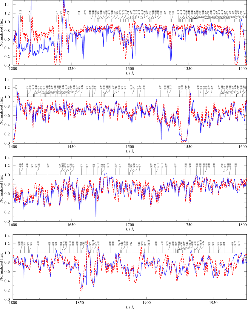
Figure 32: Ultraviolet spectrum of Vela X-1 (blue), and the best fit model (red).

The IUE is provided with two spectrographs (long-wavelength in the range $1850-3300$ Å and short- wavelength in $1150-2000$ Å) and four cameras (prime and redundant camera, for each spectrograph). Each spectrograph can be used with either large aperture (a slot 10x20 arcsec), or small aperture (a circle $3$ arcsec diameter). In addition, each spectrograph has two dispersion modes: high resolution and low resolution. High resolution mode ($\sim 0.2$ Å) utilizes an echelle grating plus a cross-disperser. Low resolution mode ($\sim 6$ Å) utilizes only the cross-disperser. IUE provides flux calibrated data. This is an important advantage due to two main reasons: first, we used these observations to fit the spectral energy distribution from the models, as explained below in Sect. 4.2; and second, we did not have to normalize the UV spectrum. As we can see in Fig. 32 and 10, it is not straightforward to see the actual flux level of the UV continuum, since this spectral range is almost completely covered by spectral lines. Therefore, any normalization by visual inspection would lead to significant errors. Instead, we rectified the IUE spectra using the PoWR model continuum.

FEROS is a spectrograph that yields high resolution echelle spectroscopy ($R\sim 48000$) and high efficiency ($\sim 20\%$) in the optical wavelength range ($3600-9200$ Å) (Kaufer et al. 1999). SpeX is an infrared spectrograph in the $0.8-5.5$ $\mu$m range. Among the different modes available in this instrument, we used the $0.8-2.4$ $\mu$m cross-dispersed mode (SXD), which yields moderate spectral resolution ($R\sim 2000$) (Rayner et al. 2003).

In Table 1 we present the set of observations of IGR J17544-2619. We used an observation from SpeX taken on August 8, 2004. In the ESO archive there are 14 FEROS observations of IGR J17544-2619 taken on four different dates during September 2005. There are not IUE available public observations of IGR J17544-2619.

In Table 2 we present the set of observations of Vela X-1. In the ESO archive there are six consecutive FEROS observations of 700s taken on April 22, 2006. For the IUE data, we used the high dispersion and large aperture observations using the short-wavelength spectrograph (1150-2000 Å) and the prime camera (SWP). There are 49 observations in the public database of the IUE following these criteria.

For each instrument, we averaged over all the available observations taking into account the exposure time in order to improve the signal-to-noise ratio. We did not take the variability of the UV spectral lines depending on the orbital phase into account, that has been reported for Vela X-1 (Sadakane et al. 1985). The variability consists on the presence of an extra absorption component in several spectral lines, specially ones belonging to Al iii and Fe iii , mainly at phases $\phi>0.5$. This variability must be taken into account to interpret the full picture of the stellar wind of Vela X-1. However, in this work, we prioritized a signal-to-noise ratio as high as possible over fitting a number of phase dependent spectra with significantly lower signal-to-noise. This permits us to estimate the stellar parameters of Vela X-1 more accurately, while not affecting any of the conclusions derived in this work, as we have carefully examined.

Instrument	Phase	Date	MJD	Exposure
		(YYYY-MM-DD)		(s)
SpeX	0.65	2004-08-15	53232.29	60
	0.01	2005-09-30	53643.05	1470
	0.01	2005-09-30	53643.03	1470
	0.01	2005-09-30	53643.01	1470
	0.02	2005-09-30	53643.07	1470
	0.61	2005-09-28	53641.08	1470
	0.61	2005-09-28	53641.06	1470
FEROS	0.61	2005-09-28	53641.04	1470
	0.62	2005-09-28	53641.10	1470
	0.74	2005-09-09	53622.01	1470
	0.75	2005-09-09	53622.02	1470
	0.76	2005-09-09	53622.10	1470
	0.76	2005-09-09	53622.08	1470
	0.97	2005-09-15	53628.06	1470
	0.98	2005-09-15	53628.08	1470

Table 1: Table of observations of IGR J17544-2619. We used $T_{90}=T_{0}=T_{\phi=0}=55924.271$ (MJD) and orbital period $P_{\text{orb}}=4.9272$ d (Drave et al. 2014).

Instrument	Phase	Date	MJD	Exposure
		(YYYY-MM-DD)		(s)
	0.05	1978-05-05	43633.62	9000
	0.07	1984-02-19	45749.32	8280
	0.08	1985-05-03	46188.67	4500
	0.09	1985-05-03	46188.75	4500
	0.09	1985-05-03	46188.81	3300
	0.10	1985-05-03	46188.86	1020
	0.10	1985-05-03	46188.92	6000
	0.10	1993-11-08	49299.55	8400
	0.14	1978-12-07	43849.51	8400
	0.17	1992-11-06	48932.56	10800
	0.22	1993-11-09	49300.55	8100
	0.28	1983-01-22	45356.80	10800
	0.28	1992-11-07	48933.57	9600
	0.29	1983-01-22	45356.91	4500
	0.29	1984-02-21	45751.31	9000
	0.33	1993-11-10	49301.55	9000
	0.40	1984-02-22	45752.36	9000
	0.40	1988-02-22	47213.55	8460
	0.41	1992-11-08	48934.72	9900
	0.45	1978-04-30	43628.21	10800
	0.46	1982-12-19	45322.52	9000
	0.46	1993-11-11	49302.71	8400
	0.49	1985-05-07	46192.36	7200
	0.50	1985-05-07	46192.47	7200
	0.51	1985-05-07	46192.58	7200
SWP	0.52	1988-02-23	47214.54	8460
	0.52	1988-03-12	47232.54	7826
	0.53	1978-12-20	43862.03	7800
	0.53	1983-01-07	45341.09	10800
	0.55	1993-11-03	49294.56	6000
	0.60	1978-12-02	43844.71	5400
	0.61	1983-01-16	45350.77	10800
	0.66	1993-11-04	49295.55	8400
	0.71	1978-12-03	43845.69	8400
	0.73	1984-02-16	45746.31	9000
	0.74	1983-01-09	45343.01	10800
	0.75	1985-04-21	46176.77	7200
	0.76	1985-04-21	46176.86	4500
	0.77	1979-03-21	43953.77	9000
	0.77	1985-04-21	46176.99	6900
	0.79	1993-11-05	49296.71	7500
	0.84	1984-02-17	45747.32	9000
	0.85	1978-07-23	43712.49	7500
	0.90	1993-11-06	49297.73	6600
	0.97	1983-01-11	45345.10	10800
	0.97	1983-01-20	45354.07	5400
	0.97	1984-02-18	45748.49	7500
	0.98	1983-01-20	45354.13	3300
	0.99	1993-11-07	49298.54	9600
	0.68	2005-04-22	53482.05	700
	0.68	2005-04-22	53482.06	700
FEROS	0.68	2005-04-22	53482.07	700
	0.68	2005-04-22	53482.07	700
	0.68	2005-04-22	53482.09	700
	0.68	2005-04-22	53482.10	700

Table 2: Table of observations of Vela X-1. We used $T_{90}=T_{0}=T_{\phi=0}=52974.001$ (MJD) and orbital period $P_{\text{orb}}=8.964357$ d (Kreykenbohm et al. 2008).

3 The PoWR code

PoWR computes models of hot stellar atmospheres assuming spherical symmetry and stationary outflow. The non-LTE population numbers are calculated using the equations of statistical equilibrium and radiative transfer in the co-moving frame. Since these equations are coupled, the solution is iteratively found. Once convergence is reached, the synthetic spectrum is calculated integrating along the emergent radiation rays. The main features of the code have been described by Gräfener et al. (2002) and Hamann & Gräfener (2003).

The basic input parameters in PoWR are the following: stellar temperature ($T_{\star}$), luminosity ($L_{\star}$), mass-loss rate ($\dot{M}$), surface gravity ($g_{\star}$) and chemical abundances. The chemical elements taken into account are detailed in Table 4. The stellar radius ($R_{\star}$) follows from $T_{\star}$ and $L_{\star}$ using the Stefan-Boltzmann law: $L_{\star}=4\pi\sigma T_{\star}^{4}R_{\star}^{2}$, where $\sigma$ is the Stefan-Boltzmann constant. We note that, in PoWR, $R_{\star}$ refers to the layer where the Rosseland continuum optical depth $\tau_{\textrm{max}}=20$, and not to the definition of stellar radius (or photospheric radius), where $\tau_{\textrm{Ross}}=2/3$. Nevertheless, we will give the stellar parameters in the next sections referring to both $\tau_{\textrm{max}}=20$ and the $\tau_{\textrm{max}}=2/3$, in order to avoid any confusion (e.g., we will use $R_{\star}$ for the radius at $\tau_{\textrm{max}}=20$ and $R_{2/3}$ for the radius at $\tau_{\textrm{max}}=2/3$). The surface gravity $g_{\star}$ and $R_{\star}$ imply the stellar mass ($M_{\star}$) via $g_{\star}=GM_{\star}R_{\star}^{-2}$. Instead of $g_{\star}$, one may specify the effective surface gravity $g_{\text{eff}}$, which accurately accounts for the outward force exerted by the radiation field, as thoroughly described by Sander et al. (2015).

The density stratification in the stellar atmosphere, $\rho(r)$, is calculated from the continuity equation $\dot{M}=4\pi r^{2}\varv(r)\rho(r)$, given $\dot{M}$ and the radial velocity stratification $\varv(r)$. For $\varv(r)$, PoWR distinguish between two different regimes: the quasi-hydrostatic domain and the wind domain. A detailed description of the quasi-hydrostatic domain can be found in Sander et al. (2015). In the wind domain, the $\beta$-law is adopted (Castor et al. 1975):

$$\varv(r)=\varv_{\infty}\left(1-\frac{r_{0}}{r}\right)^{\beta}$$ (1)

where $\varv_{\infty}$ is the terminal velocity of the wind, $r_{0}\approx R_{\star}$ (depending on the precise location of the connection point) and $\beta$ is an input parameter typically ranging between $\beta=0.6-2.0$ (Puls et al. 2008). The connection point is chosen in order to ensure a smooth transition between the two domains. The temperature stratification is calculated from the condition of radiative equilibrium (Hamann & Gräfener 2003).

The code also permits to account for density inhomogeneities and additional X-rays from a spherically-symmetric, shock heated plasma. Density inhomogeneities are described in PoWR by means of an optional radial-dependent input parameter: the density contrast $D(r)=\rho_{cl}/\bar{\rho}$, where $\rho_{cl}$ is the density of the clumped medium and $\bar{\rho}$ is the average density. The inter-clump medium is assumed to be empty. During the analysis, $D(r)$ is assumed to grow from $D(r_{\text{sonic}})=1$ (smooth plasma) to a maximum value $D$, which is reached at the layer where the stellar wind velocity is $\text{f}_{\text{max}}\times\varv_{\infty}$. $D$ is a free parameters derived in the analysis. $\text{f}_{\text{max}}$ has a modest influence on the spectra. We assumed $\text{f}_{\text{max}}\sim 0.6$ on the basis of this moderate effect. The X-rays are described using three parameters: the X-ray temperature $T_{\text{X}}$, the filling factor $X_{\text{F}}$ (i.e. the ratio between shocked to unshocked plasma), and the onset radius $R_{X}$, as described in Baum et al. (1992). In this work, we assumed $T_{\text{X}}=10^{7}$ K, $R_{X}=1.2\,R_{\star}$ and $X_{\text{F}}=0.05$. The main influence of X-rays in the model is via Auger ionization, which is responsible for the appearance of resonance lines belonging to high ions such as Nv and Ovi in the spectra of O stars (Cassinelli & Olson 1979; Krtička & Kubát 2009; Oskinova et al. 2011). Any changes in these parameters barely affect the spectrum, as long as they they produce a similar X-ray luminosity.

During the iterative calculation of the population numbers, the spectral lines are taken to be Gaussian with a constant Doppler width of $\varv_{\text{Dop}}=40\,$km/s; the effect of $\varv_{\text{Dop}}$ on the spectrum is negligible for most lines (see discussion by Shenar et al. 2015). During the formal integration, the line profiles include natural broadening, pressure broadening, and Doppler broadening. The Doppler width is decomposed per element to a depth dependent thermal motion and a microturbulent velocity $\xi(r)$. The photospheric microturbulence, $\xi_{\text{ph}}$, is derived in the analysis, and beyond the photosphere we assumed that it grows from $\xi=\xi_{\text{ph}}$ to $\xi=100$ km/s at the layer where the stellar wind velocity is $500$ km/s. Rotational broadening is simulated via convolution with rotational profiles with a width corresponding to the projected rotational velocity $\varv_{\text{rot}}\,\sin i$ (denoted by $\varv_{\text{rot}}$ hereafter for simplicity), except for important wind lines, for which the convolution is no longer valid (see e.g. Hillier et al. 2012), and where an explicit angle-integration would be required (as described by Shenar et al. 2014). The so-called macroturbulence $\varv_{\text{mac}}$ is accounted for by convolving the spectra with so-called Radial-Tangential profiles (Gray 1975; Simón-Díaz & Herrero 2007).

4 The fitting procedure

We used the PoWR code to calculate synthetic spectra and a Spectral Energy Distribution (SED) which best match the observations. The large number of free parameters, together with the long computation time for each model, do not permit the construction of a grid of models that covers the full parameter space. Instead, we attempted to identify the best-fitting model by visual inspection and systematic variation of the parameters. As an initial step, we calculate models using typical parameters of late O / early B stars. We then use specific spectral lines for each parameter as a guideline for the fit. Generally, the effective gravity $g_{\text{eff}}$ is derived from the pressure-broadened wings of the Balmer lines and He ii lines. The temperature $T_{\star}$ is derived based on line ratios belonging to different ions of the same element. The mass-loss rate $\dot{M}$, $\varv_{\infty}$ and $D$ are derived from ”wind-lines”, with $D$ adjusted so that a simultaneous fit is obtained for both resonance lines (which scale as $\rho$) and recombination lines such as H$\alpha$ (which scale as $\rho^{2}$). The luminosity $L_{\star}$ and the reddening $E_{B-V}$ are derived by fitting the SED to photometry and flux-calibrated spectra. We apply the reddening law by Fitzpatrick (1999). Abundances are estimated from the overall strengths of the spectral lines. The photospheric microturbulence $\xi_{\text{ph}}$ is found from the strength and shape of helium lines. Finally, the parameters $\beta$, $\varv_{\text{rot}}$ and $\varv_{\text{mac}}$ are adopted on the basis of the shape and depth of the spectral lines, together with previous estimations found in the literature, when available. Upon adjusting the model, the whole spectral domain was examined to iteratively improve the fit. Overall, we managed to find models which satisfactorily reproduce the observed spectra and SEDs of the donors of the two systems analysed here.

We show the complete fits in Appendix B. The details about the fitting procedure for the two objects are given in the following subsections. The obtained parameters are summarised in Table 3 and the chemical abundances in Table 4. The parameters that do not include an error estimation in the tables are adopted following the above mentioned criteria.

Even though the optical companion in Vela X-1 is usually known as HD 77581, for the sake of simplicity we will refer to the donors with the name that is used for the X-rays sources, namely, IGR J17544-2619 and Vela X-1. Depending on the context, the reader should easily recognize whether it is the donor or the X-ray source which is being referred to.

Parameters	J17544-2619	Vela X-1
$\text{log}\,(L_{\star}/L_{\odot})$	$5.4\pm 0.1$	$5.5\pm 0.1$
$M_{\star}/M_{\odot}$	$25.9\pm 2.0^{b}$	$21.5\pm 4.0$
$R_{\star}/R_{\odot}$	$20_{-3}^{+4}$	$28.4^{a}$
$R_{2/3}/R_{\star}$	$1.04$	$1.09$
$T_{\star}$ (kK)	$29.0\pm 1.0$	$25.5\pm 1.0$
$T_{2/3}$ (kK)	$28.5\pm 1.0$	$24.4\pm 1.0$
$\text{log}\,(g_{\star}\,\text{(cgs)})$	$3.25\pm 0.20$	$2.86\pm 0.10$
$\text{log}\,(g_{\text{eff}}\,\text{(cgs)})$	$2.80\pm 0.20$	$2.35\pm 0.10$
$\text{log}\,(g_{\text{eff \, 2/3}}\,\text{(cgs)})$	$2.77\pm 0.20$	$2.27\pm 0.10$
$\varv_{\infty}$ (km/s)	$1500\pm 200$	$700_{-100}^{+200}$
$\varv_{\text{esc}}$ (km/s)	$618\pm 75$	$436\pm 65$
$\text{log}\,(\dot{M}/(M_{\odot}/yr))$	$-5.8\pm 0.2$	$-6.2\pm 0.2$
$D$	$4$	$11\pm 5$
$\xi_{\text{ph}}$ (km/s)	$25\pm 10$	$30\pm 10$
$\beta$	$0.8$	$1.0$
$\varv_{\text{mac}}$ (km/s)	$60$	$80$
$\varv_{\text{rot}}$ (km/s)	$160$	$56^{c}$
$E_{\text{B-V}}$	$2.14\pm 0.10$	$0.77\pm 0.05$
$R_{\text{V}}$	$2.9$	$3.1$
$d$ (kpc)	$3.0\pm 0.2$	$2.0\pm 0.2$

Table 3: Stellar parameters obtained from the best fit. (a) Joss & Rappaport (1984). (b) Pellizza et al. (2006). (c) Fraser et al. (2010)

	IGR J17544-2619		Vela X-1
Quemical Element	Mass Fraction	Rel. Ab.	Mass Fraction	Rel. Ab.
H	$(6.2\pm 0.5)E-01$	$0.85$	$(6.5\pm 0.5)E-01$	$0.89$
He	$(3.7\pm 0.5)E-01$	$1.47$	$(3.4\pm 0.5)E-01$	$1.35$
C	$(5.0\pm 3.0)E-04$	$0.17$	$(5.0\pm 3.0)E-04$	$0.17$
N	$(2.2\pm 0.6)E-03$	$2.58$	$(1.8\pm 0.6)E-03$	$2.11$
O	$(6.0\pm 2.0)E-03$	$0.76$	$(7.0\pm 0.2)E-03$	$0.88$
Si	$(7.3\pm 2.0)E-04$	$1.00$	$(5.5\pm 2.0)E-04$	$0.75$
S	$5.0E-04$	$1.00$	$5.0E-04$	$1.00$
P	$6.4E-06$	$1.00$	$6.4E-06$	$1.00$
Al	$5.8E-05$	$1.00$	$7.0E-05$	$1.00$
Mg	$7.0E-04$	$1.00$	$7.0E-04$	$1.00$
$\text{Fe}^{a}$	$1.4E-03$	$1.00$	$1.4E-03$	$1.00$

Table 4: Chemical abundances derived from the best fit, in mass fraction and relative to solar abundances from Asplund et al. (2009). (a) The notation of Fe actually stands for a generic atom including iron group elements Sc, Ti, V, Cr, Mn, Co and Ni. For more details see Gräfener et al. (2002).

4.1 IGR J17544-2619

IGR J17544-2619 was first detected on September 2003 with the IBIS/ISGRI detector on board INTEGRAL (Sunyaev et al. 2003). It is located in the direction of the galactic center, at galactic coordinates $l=3.24^{\circ}$, $b=-0.34^{\circ}$. The orbital period is $\sim$4.9d (Clark et al. 2009). According to Chandra observations, the compact object is a neutron star (in’t Zand 2005). Pellizza et al. (2006) used optical and NIR observations in order to classify the optical companion as a O9Ib. Chandra and Swift observations showed that the system exhibits a high dynamic range in its X-ray variability, changing the X-ray flux by 5 orders of magnitude (in’t Zand 2005; Romano et al. 2015).

Nowadays, the spin period $P_{\text{spin}}$ of the hypothetical neutron star in IGR J17544-2619 is a matter of debate, given the results arising from observations taken at different times, different luminosities and different instruments. Drave et al. (2012) analysed RXTE data of the source at intermediate X-ray luminosity ($\sim 10^{33-34}$ erg/s), and reported the detection of an X-ray pulsation with $P_{\text{spin}}=71.49$s at a statistical significance of $4.37\sigma$. Romano et al. (2015) inspected Swift observations of the source experiencing an extraordinarily bright outburst (peak luminosity $\sim 10^{38}$ erg/s), and reported the detection of X-ray pulsations with $P_{\text{spin}}=11.60$s at a statistical significance of about $4\sigma$ too. However, these results contrast with the analyses of XMM-Newton and NuSTAR observations performed by Drave et al. (2014) and Bhalerao et al. (2015) respectively. These authors do not find any evidence of pulsations on time scales of 1-2000s.

We have adjusted T_⋆ of IGR J17544-2619 using different ions, mainly He i-He ii and Si iii-Si iv. In Fig. 1 we show an example of four helium lines of which the best-fit model provides a good description. Higher (lower) temperatures yield more (less) absorption than observed in the He ii lines. We have used other lines of helium, silicon, nitrogen and oxygen. The vast majority of them are well described by the best-fit model, within the errors. The obtained effective temperature is compatible with the donor’s spectral class O9 Ib (Martins et al. 2005).

Figure 1: Example of four helium lines in IGR J17544-2619, used for the estimation of T_⋆. We show the observation (solid blue line), the best-fit model (red dashed line), a model with lower temperature of $T_{\star}=28$ kK (green dashed line), and a model with higher temperature of $T_{\star}=30$ kK (pink dashed line).

The effective gravity g${}_{\text{eff}}$ was found using the hydrogen Balmer lines H$\gamma$ and H$\delta$. We did not use H$\beta$ and H$\alpha$ because these lines are notably affected by the stellar wind. Figure 2 shows a comparison of the observations with the best-fitting model for these two Balmer lines. We show that the observations are compatible with a relatively wide range of values, as also reflected in the errors given in Table 3.

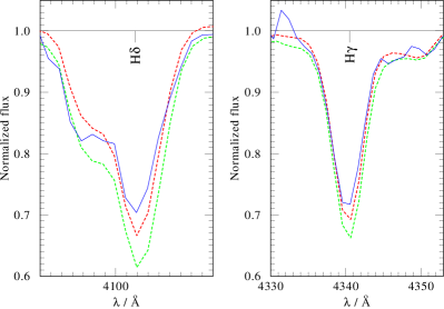
Figure 2: H$\gamma$ and H$\delta$ in IGR J17544-2619, used for the surface gravity estimation. We show the observation (solid blue line), the best-fit model (red dashed line) and a model with larger effective gravity of $\text{log}\,(g_{\text{eff}})=3.0$ in cgs units (green dashed line).

The distance to IGR J17544-2619 is not well known, with an estimate of 2-4 kpc Pellizza et al. (2006), based on the extinction and the calibration of the absolute magnitude for O9Ib stars. In this work we improve this estimation. As a first step, we fitted the SED to photometry from the 2MASS catalogue (Cutri et al. 2003), Zacharias et al. (2012) and Rahoui & Chaty (2008) assuming the distance to be 3 kpc. Then, we derived initial values for the luminosity of the donor and the reddening to the system.

As a second step, in order to provide more constraints on the distance, we employed a method based on the well constrained luminosity of Red Clump Giant stars (RCG). These stars can be isolated in a NIR colour-magnitude diagram and permit the estimation of the interstellar extinction along the line of sight (López-Corredoira et al. 2002). Due to their narrow luminosity function, the apparent magnitude of RCGs provides an estimation of the distance. Then, given a certain line of sight, a diagram of the extinction versus the distance can be derived (for more details see González-Fernández et al. 2014). For IGR J17544-2619 we employed the derived $E_{J-K}$ from the SED fit to obtain an estimate of the distance. We note that this method is only applicable to stars in the direction of the galactic center like IGR J17544-2619, where the medium is more homogeneous and the density of RCGs is higher. Using this method, we obtain a distance of $3.0\pm 0.2$ kpc (Fig. 3). Revised values for the luminosity and reddening are then derived. The final results of the SED fit are shown in Fig. 4.

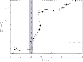
Figure 3: Extinction curve in the galactic direction of IGR J17544-2619. The shaded area reflects the error in the distance estimation from the errors of estimation of the extinction and the errors in the calculation of the extinction curve.

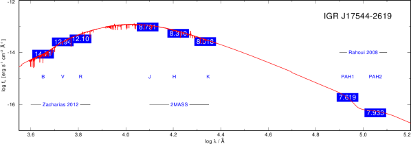
Figure 4: Fit of the SED of IGR J17544-2619. In red we plot the best-fit model. We indicate the photometry values for each band in blue. The employed references are cited. The values of extinction, distance and luminosity are shown in Table 3.

From the luminosity and temperature we derive $R_{\star}$, which provides an upper limit to the eccentricity of the system. For the lower limit $R_{\star}=17\,R_{\odot}$, we find $e<0.25$. For higher eccentricities, periodic Roche-lobe overflow is expected from the orbital solution of the system (Clark et al. 2009), at odds with the X-ray behavior of the source. Given the radius of the source and the derived surface gravity, we find $M_{\star}=25.9\,M_{\odot}$. This value matches very well with the estimation of $M_{\star}=25-28\,M_{\odot}$ done by Pellizza et al. (2006) based on the mass calibration with its spectral type.

The terminal velocity of the stellar wind $\varv_{\infty}$ was derived using the P-Cygni profile of He i $\lambda 10833\,\AA$ (see Fig. 5). The blue wing in He i $\lambda 10833\,\AA$ is a very good indicator due to its strong sensitivity to $\varv_{\infty}$. It is reasonably well fitted when assuming $\varv_{\infty}\simeq 1500$ km/s. Unfortunately, the emission exhibited by this line is not well reproduced by the best-fit model, as explained below.

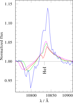
Figure 5: He i at $\lambda\,10833\,\AA$, used for the estimation of $\varv_{\infty}$ in IGR J17544-2619 fitting the blue wing of the P-Cygni profile. We show the observation (solid blue line), the best-fit model (red dashed line), a model with $\varv_{\infty}=1300$ km/s (green dashed line), and a model with $\varv_{\infty}=1700$ km/s (pink dashed line).

The $\dot{M}$ and $D$ were simultaneously adjusted by means of H$\alpha$ and the P-Cygni profile of HeI $\lambda 10833$ Å. Provided that the strength of emission in these recombination spectral lines varies with $\dot{M}\sqrt{D}$ (Gräfener et al. 2002), we cannot estimate $\dot{M}$ and $D$ independently using these lines. As it is shown in Fig. 6, we were not able to fit all the lines at the same time. The best-fit model provides an acceptable description of H$\alpha$, but yields insufficient emission for HeI $\lambda 10833$ Å. We choose the best description of H$\alpha$ as the best-fit because it provides a better fit to the overall spectrum. We note that the optical and infrared spectra were not taken at the same time, and therefore any kind of variability in the lines might produce a disagreement. However, H$\alpha$ does not show such a large variability within the observations we have analysed (see Fig. 7).

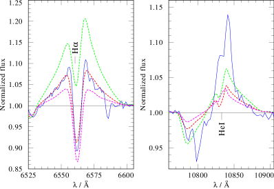
Figure 6: H$\alpha$ and He i $\lambda 10833\AA$ lines for the estimation of $\dot{M}\sqrt{D}$ in IGR J17544-2619. We show the observation (solid blue line), the best-fit model (red dashed line), a model with higher $\dot{M}\sqrt{D}$ ($1.35$ times the best-fit value, green dashed line), and a model with lower $\dot{M}\sqrt{D}$ ($0.8$ times the best-fit value, pink dashed line).

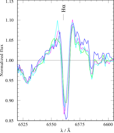
Figure 7: H$\alpha$ in IGR J17544-2619 at different orbital phases: $\phi\simeq 0.01,0.61,0.75,0.97$ (blue, green, pink and turquoise solid lines respectively).

Without available resonance scattering lines in the observations at hand, we cannot compare P-Cygni lines with recombination lines to deduce the clumping factor $D$. However, our calculations show that changing $\dot{M}$ dramatically affects the absorption spectrum in a fashion which is not related to the product $\dot{M}\sqrt{D}$. An example is shown in Fig. 8, where we show three models calculated with different values of $\dot{M}$ and $D$, but with a fixed product $\dot{M}\sqrt{D}$. Evidently, while the emission exhibited by the wings of H-$\alpha$ (shown in Fig. 8) is similar in all models, the absorption lines are strongly affected in a non-trivial manner. The reason for this unexpected behaviour is that many of the strong lines in the spectrum (e.g. the Balmer series) are formed significantly beyond the photosphere ($\tau_{\rm Ross}\approx 2/3$), where the mass-loss rate already strongly affects the density stratification via the continuity equation. Exploiting this effect, we find that $D\approx 4$ provides the best results for the overall spectrum. However, we warn that further observations are needed to better constrain the clumping factor in this star. Nevertheless, we note that our final conclusions do not strongly depend on this factor and the implied mass-loss rate, as will be discussed in Section 5.

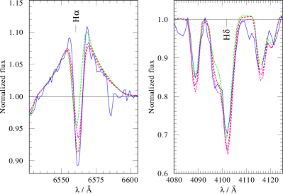
Figure 8: H$\alpha$ and H$\delta$  for the estimation of $\dot{M}$ in IGR J17544-2619. We show the observation (solid blue line), the best-fit model ($\dot{M}=10^{-5.8}\,M_{\odot}/yr$, $D=4$, red dashed line), a model with higher $\dot{M}$ ($\dot{M}=10^{-5.5}\,M_{\odot}/yr$, $D=1$, green dashed line), and a model with lower $\dot{M}$ ($\dot{M}=10^{-5.9}\,M_{\odot}/yr$, $D=8$, pink dashed line). Different $\dot{M}$ values do not yield different H$\alpha$ wings as long as the product $\dot{M}\sqrt{D}$ remains constant. However, we observed that other important lines like H$\delta$ are sensitive these variations.

The chemical composition was estimated from unblended spectral lines for He, C, N, O and Si. The rest of the considered element abundances (see Table 4) were assumed solar following Asplund et al. (2009). The fit yielded moderate overabundance of He and N, together with underabundance of C and O. In all, there are indications of chemical evolution in the outer layers of the stellar atmosphere.

The photospheric microturbulent velocity ($\xi_{\text{ph}}$) was adjusted using He i and Si iv lines. A higher $\xi_{\text{ph}}$ induce stronger absorption in several spectral lines, as shown in Fig. 9.

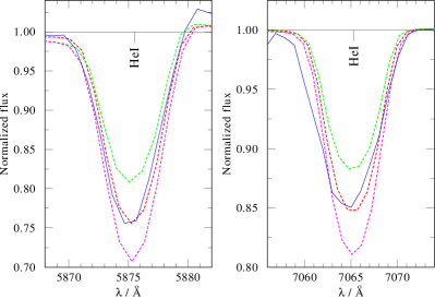
Figure 9: Example of two He i lines in IGR J17544-2619, used in the $\xi_{\text{ph}}$ estimation. As usual, the observation is plotted in solid blue line, and the best-fit model in red dashed line. Models with $\xi_{\text{ph}}=15,35$ km/s are also presented (green and pink dashed lines respectively).

The $\varv_{\text{rot}}$ and $\varv_{\text{mac}}$ were roughly estimated using the width of the He lines. The derived projected rotational velocity is around 0.3 times the critical rotation velocity ($\varv_{\text{crit}}=\sqrt{G\,M_{\star}R^{-1}_{\star}}$). This high rotational velocity may favour the chemical mixing, in line with the abundances derived in the fit.

To summarise, our NLTE analysis of optical and near IR spectra of IGR J17544-2619 showed that the optical O9I-type companion in this source is not peculiar and has stellar and wind parameters that are similar to other stars of the same spectral type, e.g. $\delta$ Ori (Shenar et al. 2015).

4.2 Vela X-1

Vela X-1 is one of the most studied HMXBs, since it is a bright source discovered in the early ages of the X-ray astronomy (Chodil et al. 1967). It is located at galactic coordinates $l=263.06^{\circ}$, $b=3.93^{\circ}$. The distance was estimated to be $1.9\pm 0.2$ kpc by (Sadakane et al. 1985). The system has a moderate eccentricity of $e=0.09$ (Bildsten et al. 1997), and orbital period $P_{\text{orb}}=8.96$ days (Kreykenbohm et al. 2008). The compact object is a neutron star that pulsates with $P_{\text{spin}}=283$s (McClintock et al. 1976). The optical companion HD 77581 (B0.5Iae) was identified by Vidal et al. (1973).

It is very likely that the wind of Vela X-1 is disturbed by the X-ray source. The photoionization produced close to the photosphere due to the intense X-ray luminosity might hinder the acceleration of the wind and generate a structure known as photoionization wake (Blondin et al. 1990; Krtička et al. 2015). This structure appears in the UV spectra as an additional absorption component at phases larger than $\phi\sim 0.5$ (Kaper et al. 1994). In addition, the hard X-rays light curves of the source in near-to-eclipse phases show asymmetries between ingress and egress, that have been interpreted as caused by the existence of this type of structure trailing the neutron star (Feldmeier et al. 1996). Moreover, a density enhancement in the line of sight during the second half of the orbit is also observed in the X-rays absorption, although the amount of absorbing material is highly variable from one orbit to another.

We derived $T_{\star}$ following the same procedure that we used for IGR J17544-2619. The obtained $T_{2/3}$ is similar to previous estimations: Sadakane et al. (1985) used the equivalent width (EW) of photospheric lines to estimate the effective temperature $T_{2/3}=25000$ K; Fraser et al. (2010) used the TLUSTY code to estimate $T_{2/3}=26500$ K.

For the fit of the SED, we used photometry from the 2MASS catalogue (Cutri et al. 2003) and the Stellar Photometry in Johnson’s 11-color system (Ducati 2002), together with the IUE observations. We made an estimation of the reddening, distance and $R_{\text{V}}\equiv A(V)/E_{B-V}$ by means of the SED fit. Then, we used the estimation of the stellar radius $R_{2/3}=31\,R_{\odot}$ from Joss & Rappaport (1984), and $T_{2/3}$ from the successive fits, in order to derive the luminosity (and the distance estimation) from the Stefan-Boltzmann law. Given that the obtained T_2/3 is very similar to previous estimations, the derived distance of $2.0\pm 0.2$ is almost equal to the value d=1.9 kpc given by Sadakane et al. (1985). We show the results of the SED analysis in Fig. 10.

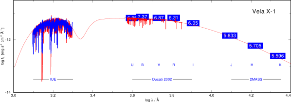
Figure 10: Fit of the SED of Vela X-1. In red we plot the best fit model with the spectral lines in the domain where we have done the spectral analysis, and the continuum where we have available photometry (marked in blue). We cite the references used for the photometry. Note that the true continuum in the UV range do not correspond with the apparent continuum from the observation, due to the number of spectral lines in this domain. The employed values of extinction, distance and luminosity are shown in Table 3.

The estimation of g${}_{\text{eff}}$ was especially delicate in Vela X-1 because of its very low g${}_{\text{eff}}$. A higher value beyond the error given in Table 3 has a strong effect in the overall spectrum and hinders a satisfying fit. The derived value enables a good fit, and it is in agreement with previous estimations (Fraser et al. 2010).

We used UV resonance lines to find $\varv_{\infty}$. In Fig. 11 we show the Si iv resonance lines $\lambda\,1394,1403\,\AA$, where the effect of $\varv_{\infty}$ is very clear. Models with higher terminal velocities induce a shift towards the blue part of these spectral lines. The best description of the observations is achieved for $\varv_{\infty}=700$ km/s. This value is in agreement with the estimation of van Loon et al. (2001): $\varv_{\infty}=600$ km/s; and not too far from Watanabe et al. (2006), who estimated $\varv_{\infty}=1100$ km/s using Chandra X-rays observations.

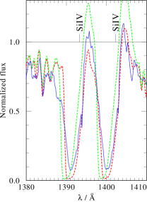
Figure 11: Si iv lines used for the estimation of $\varv_{\infty}$ in Vela X-1. It is showed the observation (blue solid line), the best-fit model (red dashed line) and a model with $\varv_{\infty}=900$ km/s (green dashed line).

In contrast, it is in disagreement with the estimation of Dupree et al. (1980), namely $\varv_{\infty}=1700$ km/s. These authors used a subset of the IUE observations used in this work, and considered the UV resonance lines Si iv and C iv in the X-ray eclipse phases to make their estimation. We have revisited our $\varv_{\infty}$ estimation using only observations taken at orbital phases $\phi=0.9-0.1$, in order to be able to directly compare to Dupree et al. (1980). In Fig. 12, we show the Si iv and C iv lines, as observed in the total averaged spectrum and the spectrum averaging over $\phi=0.9-0.1$. C iv is almost the same in both cases. Then, the disagreement in the estimates of $\varv_{\infty}$ does not come from orbital phase variations but from the omission of the impact of the X-rays in the stellar wind by Dupree et al. (1980). As we can see in Fig. 12, when we introduce X-rays in the models we are able to reproduce C iv without needing a high velocity, due to the significant enhancement of the population of C iv in the wind. We note that the X-ray radiation we are introducing in the models is an intrinsic radiation of the donor wind that is presumably produced in the shocks within the stellar wind itself (e.g. Krtička et al. 2009). This radiation is not coming from the neutron star, since the effects are also noticeable at eclipsing phases. The impact of the X-rays coming from the neutron star is a different and complex issue, and it has been already studied by other authors (Watanabe et al. 2006). Regarding the Si iv resonance lines, in Fig. 12 we show that high stellar wind velocities as derived by Dupree et al. (1980) do not fit, neither using the total averaged spectrum, neither using the eclipsing phases spectrum.

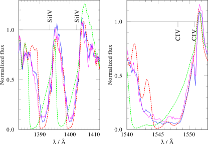
Figure 12: Si iv and C iv resonance lines. We plot the total averaged spectrum (blue solid line) and the averaged spectrum over orbital phases $\phi=0.9-0.1$ (pink solid line). We also plot the best-fit model ($\varv_{\infty}=700$, red dashed line), and a model with $\varv_{\infty}=1400$ km/s (green dashed line).

The value $\dot{M}\sqrt{D}$ was estimated using H$\alpha$ (see Fig. 13). We did not find a good fit of the blue wing of the line, observed in absorption, but our model properly fits the emission in the red wing of the spectral line. Unfortunately, we do not have more optical observations covering further orbital phases in order to check whether H$\alpha$ is variable. Nevertheless, previous studies of similar sources demonstrate that this might be the case: González-Galán (2015) reported the variability of H$\alpha$ in the very similar B0Iaep optical companion in the SGXB system XTE J1855-026. Moreover, the shape of H$\alpha$ in XTE J1855-026 at $\phi=0$ (see Fig. 5.12 in González-Galán 2015), when the neutron star is hidden behind the optical counterpart, is strongly reminiscent of the shape that our model reproduces in Fig. 13. Hence, the relative disagreement between our best-fit model and our observation of Vela X-1 (taken at $\phi=0.68$), might be produced by some kind of interaction of the neutron star with the donor and/or the stellar wind, which is not possible to model using the assumption of spherical symmetry that PoWR employs. This disagreement might be related to similar features observed in other strong lines, as further discussed in Sect. 5.3.

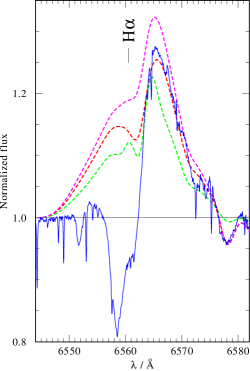
Figure 13: H$\alpha$ line for the estimation of $\dot{M}\sqrt{D}$ in Vela X-1. We can see the observation (blue solid line), the best-fit model (red dashed line), a model with $0.8$ times the $\dot{M}\sqrt{D}$ value of the best fit (green dashed line), and a model with $1.2$ times the $\dot{M}\sqrt{D}$ value of the best fit (pink dashed line).

We derived $\dot{M}$ and $D$ from the Al iii resonance lines $\lambda 1855$ and $\lambda 1863\AA$. As we can see in Fig. 14, the variation of $\dot{M}$ (and consequently $D$) directly affect these lines. Higher (lower) $\dot{M}$ enhances (reduces) the density of the stellar wind, producing too strong (weak) absorption.

Unfortunately, other resonance lines available in the spectrum (N v, C iv and Si iv) are saturated in the models within a reasonable range of parameters around the best-fit, and consequently are not suitable for the $\dot{M}$ diagnosis. Interestingly, in contrast to the models, the N v and Si iv resonance lines are slightly desaturated in the observations (see Fig. 15). The origin of this phenomenon might be related to the presence of optically thick clumps (macroclumping), which directly affects the mass-loss rate estimations (Oskinova et al. 2007; Šurlan et al. 2012). Undoubtedly, its study deserves further investigation, which is beyond the scope of this work.

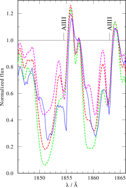
Figure 14: Al iii resonance lines $\lambda 1855$ and $\lambda 1863\AA$, employed for the $\dot{M}$ estimation in Vela X-1. We show the observation (solid blue line), the best-fit model ($\dot{M}=10^{-6.2}\,M_{\odot}/yr$, $D=11$, red dashed line), a model with higher $\dot{M}$ ($\dot{M}=10^{-5.8}\,M_{\odot}/yr$, $D=2$, green dashed line), and a model with lower $\dot{M}$ ($\dot{M}=10^{-6.3}\,M_{\odot}/yr$, $D=20$, pink dashed line).

Figure 15: Si iv and N v resonance lines in Vela X-1. While the observations show slight desaturation, all the models within a reasonable parameter space around the best-fit model produce saturated lines.

Based on the X-ray data analysis, Manousakis & Walter (2015) have suggested that the velocity law with the parameter $\beta=0.5$ fits better with the X-ray light curve of the system in near-to-eclipse phases. However, a satisfying fit is not possible when we assume $\beta=0.5$. We have tried models using $\beta=0.5$ and adapting $\dot{M}\sqrt{D}$ in order to fit H$\alpha$. However, as shown in Fig. 16, H$\alpha$ in our observation is not compatible with $\beta=0.5$. As we mentioned above, H$\alpha$ might suffer from important variability along the orbit. Moreover, the X-ray irradiation from the neutron star might produce variations in the stellar wind. In our opinion, this might be the cause of the apparent disagreement between the conclusions extracted from the X-rays and the optical wavebands.

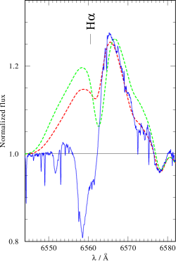
Figure 16: H$\alpha$  used the estimation of the parameter $\beta$ in Vela X-1. We present the observation (solid blue line), the best-fit model ($\beta=1.0$, red dashed line), and a model with $\beta=0.5$ (green dashed line), as proposed by Manousakis & Walter (2015).

The chemical composition was estimated following the same approach as it was done for IGR J17544-2619. Interestingly, we found again indications of chemical evolution in the star, given the moderate overabundance of He and N, together with the underabundance of C and O (see Table 4).

We adopted the value of $\varv_{\text{rot}}\,\sin i=56$ km/s derived by Fraser et al. (2010). Previous estimations pointed to much higher values around 115 km/s (Zuiderwijk 1995; Howarth et al. 1997), but such a high rotational velocity is not compatible with some of the lines that we see unblended in the optical observation (see Fig. 17). The rotational velocity directly affects the estimation of the neutron star mass ($M^{\text{NS}}_{\textsc{Vela\,X-1}}$) from radial velocity curves, as shown by Koenigsberger et al. (2012). If $\varv_{\text{rot}}\,\sin i=56$ km/s, it is feasible that $M^{\text{NS}}_{\textsc{Vela\,X-1}}\sim 1.5\,M_{\odot}$, close to the canonical value ($1.4\,M_{\odot}$), instead of a high mass neutron star $M^{\text{NS}}_{\textsc{Vela\,X-1}}\gtrsim 1.8\,M_{\odot}$, as suggested by other authors (e.g. Quaintrell et al. 2003; Barziv et al. 2001).

Figure 17: Example of unblended lines in the spectrum of Vela X-1. In red we plot a model with $\varv_{\text{rot}}\,\sin i=56$ km/s. In green we plot a model with $\varv_{\text{rot}}\,\sin i=116$ km/s.

To summarise, our new analysis of Vela X-1 is in broad agreement with previous studies of this system. We find a rather low stellar wind velocity, while $\dot{M}$ is typical for the stars of its spectral type. Like other studies, we note spectral line variability in dependence with orbital phase, and attribute it to the influence of the X-rays and the compact object on the stellar wind.

The final physical parameters of the the two sources obtained in this work are shown in Table 3.

5 Discussion

5.1 Wind-fed accretion

In SFXTs and SGXBs, the X-ray emission is powered by the accretion of matter from the donor’s wind onto the compact object. The efficiency of the conversion of the potential energy into X-ray luminosity depends on many factors including the properties of the stellar wind, the properties of the compact object and the orbital separation.

Parameters	J17544-2619	Vela X-1
$P_{\text{orb}}$ (d)	$4.9^{\text{a}}$	$8.964357^{b}$
$P_{\text{spin}}$ (s)	$71.49^{c}$, $11.58^{d}$	$283.532^{b}$
$a\,\sin i$ (lt-s)	-	$113.89^{b}$
$i$ (deg)	-	$>73^{e}$
$a$ ($10^{12}$cm)	$2.6^{i}$	$3.5^{j}$
$a$ ($R_{\star}$)	$1.9$	$1.8$
$B$ ($10^{12}$G)	$1.45^{f}$	$2.6^{g}$
$\varv_{\text{wind}}$ (km/s)	$789^{h}$	$264^{h}$
$\varv_{\text{orb}}$ (km/s)	$386^{k}$	$281^{k}$

Table 5: Parameters used in Sect. 5.
References: (a) Clark et al. (2009) (b) Kreykenbohm et al. (2008) (c) Drave et al. (2012) (d) Romano et al. (2015) (e) van Kerkwijk et al. (1995) (f) Bhalerao et al. (2015) (g) Kreykenbohm et al. (2002) (h) this work. (i) From $P_{\text{orb}}$, total mass of the system and the 3rd Kepler’s law. (j) From $a\,\sin i$, and the average $\langle\sin i\rangle=0.985$ over $i>73^{\circ}$. (k) Assuming a circular orbit.

The most efficient way of producing X-rays is the so called direct accretion: the stellar wind that is gravitationally captured by the neutron star free-falls onto the compact object. The expected luminosity is close to the accretion luminosity $L_{\text{acc}}$. The following equations contain the most relevant parameters in this regime:

$$R_{a} =\frac{2GM_{\text{NS}}}{\varv_{\text{rel}}^{2}}$$ (2a)

$$f_{a} =\frac{R_{a}^{2}}{4a^{2}}$$ (2b)

$$L_{\text{acc}} =f_{a}\,\frac{GM_{\text{NS}}\dot{M}}{R_{\text{NS}}}$$ (2c)

where $R_{a}$ is the accretion radius (also called Bondi radius), that is to say, the maximum distance to the neutron star where the stellar wind is able to avoid falling onto the compact object; $G$ is the gravitational constant; $M_{\text{NS}}$ is the mass of the neutron star, which in this work is hereafter assumed to be the canonical value $1.4\,M_{\odot}$; $R_{NS}$ is the radius of the neutron star, which in this work is henceforward assumed to be $12$ km (Lattimer & Steiner 2014); $\varv_{\text{rel}}$ is the velocity of the wind relative to the neutron star; $f_{a}$ is the fraction of stellar wind that is gravitationally captured by the neutron star; $a$ is the orbital distance and $L_{\text{acc}}$ is the accretion luminosity, namely, the luminosity that would arise if the whole potential energy of the accreted matter is eventually transformed in X-ray luminosity.

For IGR J17544-2619, using the results of our spectral fitting, the data shown in Table 5 and assuming a circular orbit, we obtain from Eq. 2c:

$$L_{\text{acc}}=1.4\cdot 10^{36}\,\text{erg/s}$$

The value of $L_{\text{acc}}$ is 1-2 orders of magnitude higher than the luminosity that the source exhibits most of the time: $L_{\text{X}}<5\cdot 10^{34}$ erg/s (Bozzo et al. 2015). Most likely, some inhibition mechanism is acting in IGR J17544-2619 (Drave et al. 2014; Bozzo et al. 2008).

As a possible explanation for the variability of IGR J17544-2619 and its lower-than-expected luminosity at quiescence, Bozzo et al. (2008) discussed the application of their model to the light curve of an outburst observed by Chandra. This theoretical framework describes the mechanisms for the inhibition of the accretion according to the relative size of the spheres defined by $R_{\text{a}}$, $R_{\text{M}}$ and $R_{\text{co}}$; where $R_{\text{a}}$ is the already defined accretion radius, $R_{\text{M}}$ is the magnetospheric radius (location where the pressure exerted by the gas equals the local magnetic pressure), and $R_{\text{co}}$ is the co-rotation radius (location where the angular velocity of the neutron star equals the Keplerian velocity). These radii, in turn, depend on: $\dot{M}$, $\varv_{\text{rel}}$, magnetic moment of the neutron star ($\mu$), orbital separation ($a$) and $P_{\text{spin}}$.

For simplicity, the orbital velocity of the neutron star and the eccentricity are not considered in the model by Bozzo et al. (2008). That is to say, it is assumed that $e=0$ and $\varv_{\text{wind}}\simeq\varv_{\text{rel}}$, where $\varv_{\text{wind}}$ is the stellar wind velocity in the position of the neutron star. We note that when the stellar wind velocity is not very high, this assumption might not be accurate. Indeed, the orbital velocity ($\varv_{\text{orb}}$) in Vela X-1 is very similar to $\varv_{\text{wind}}$ (see Table 5). In IGR J17544-2619, the orbital velocity is around the half of the stellar wind velocity. Despite these simplifications, the model provides significant insight on the explanation of the qualitative behavior of the sources with regard to their persistence or variability, as it is shown next in this section. A more accurate approach considering eccentric orbits and the orbital velocity of the compact object would be an important advance in the model, but it is out of the scope of this paper.

Nowadays, the tentative estimations of the spin period in IGR J17544-2619 ($P_{\text{spin}}=71.49$s by Drave et al. (2012) and alternatively $P_{\text{spin}}=11.58$s by Romano et al. 2015), along with the stellar wind parameters derived in this work, permit to discuss the application of the model by Bozzo et al. (2008) from a new perspective. The rest of parameters required for this section are shown in Table 5. Using those values, we can elaborate diagrams $\varv_{\text{wind}}$-$\dot{M}$ and $\varv_{\text{wind}}$-$P_{\text{spin}}$, where the different accretion regimes occupy different domains of the space of parameters. These domains directly arise from the Eq. 25-28 by Bozzo et al. (2008).

In Fig. 18 we show the position of IGR J17544-2619 in the diagram $\varv_{\text{wind}}$-$P_{\text{spin}}$ for the two currently available tentative estimations of the $P_{\text{spin}}$. The source lie in the direct accretion regime for $P_{\text{spin}}=71.49$s, and in the supersonic propeller regime for $P_{\text{spin}}=11.58$s. Hence, the shortest $P_{\text{spin}}=11.58$s matches better with the X-ray behavior of the source and its likelihood of staying in an inhibited accretion regime.

Figure 18: Position of IGR J17544-2619 in the $\varv_{\text{wind}}$-$P_{\text{spin}}$ diagram for the two tentative estimations of $P_{\text{spin}}$. Equations 25, 26, 27 and 28 by Bozzo et al. (2008) are represented by a solid, dotted, triple-dot-dashed and dot-dashed lines respectively.

In Fig. 19 we show the location of IGR J17544-2619 in the diagram $\varv_{\text{wind}}$-$\dot{M}$. It is important to note that the position of the system in this diagram is not a fixed point due to the the intrinsic variability of the velocity and local density of the stellar wind in hot massive stars. Thus, we have plotted a red region in Fig. 19 showing a variability of one order of magnitude in $\varv_{\text{wind}}$ and $\dot{M}$. That is to say, the maximum $\dot{M}$ and $\varv_{\text{wind}}$ in the encircled region is ten times higher than the minimum $\dot{M}$ and $\varv_{\text{wind}}$. Such a variability is fully plausible, as demonstrated by hydrodynamical simulations of radiatively driven stellar winds (e.g. Feldmeier et al. 1997). These clumps of higher density, intrinsic to stellar winds of hot stars, are sometimes invoked to explain the X-ray variability of HMXBs (Oskinova et al. 2012). As we can see in Fig. 19, the encircled region intersects regimes of direct accretion and inhibited accretion. Hence, it is possible that in objects like IGR J17544-2619, the abrupt changes in the wind density may lead to the switching from one accretion regime to the other. Moreover, besides the clumping of the stellar wind, the eccentricity of the orbit ($e<0.25$) would lead to additional variations in the orbital separation (and consequently in $\varv_{\text{wind}}$ and the density of the medium), which reinforce the intrinsic variability of the stellar wind and its capability to lead to transitions across regimes.

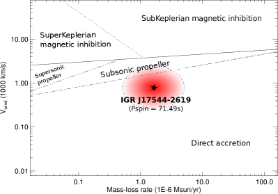
Figure 19: Position of IGR J17544-2619 in the $\varv_{\text{wind}}$-$\dot{M}$ diagram. Upper panel: diagram calculated using $P_{\text{spin}}=11.58$s. Lower panel: diagram calculated using $P_{\text{spin}}=71.49$s. The dashed line encircles the space within one order of magnitude of $\varv_{\text{wind}}$ and $\dot{M}$. Equations 25, 26, 27 and 28 by Bozzo et al. (2008) are represented by a solid, dotted, triple-dot-dashed and dot-dashed lines respectively.

Considering an alternative explanation for the X-ray variability of IGR J17544-2619, Drave et al. (2014) invoked the quasi-spherical accretion model by Shakura et al. (2012). However, if the spin period is actually as short as $71.49$s or $11.58$s, the condition of a slowly rotating pulsar, i.e. R${}_{\text{M}}\ll\text{R}_{\text{co}}$ (where R${}_{\text{M}}$ is the magnetospheric radius and R${}_{\text{co}}$ the co-rotation radius), assumed by this approach, would be debatable. Even though it raises doubts about the feasibility of applying this model, it cannot be ruled out until the spin period and the magnetic field of the neutron star are firmly constrained.

In the case of Vela X-1, we can see in Fig. 20 and  21, the source is well in the middle of the zone where direct accretion is expected. Hence, more extreme density or velocity jumps would be required to trigger any change of accretion regime. These extreme jumps are also plausible, but much more unlikely. However, they might sporadically occur and lead to a sudden decrease of the luminosity in Vela X-1.

Using the parameters shown in Table 5 and Eq. 2c, we obtain $L_{\text{acc}}=8.7\times 10^{36}$ erg/s for Vela X-1. The average X-rays luminosity of the source is $\langle L_{\text{X}}\rangle\simeq 4.5\times 10^{36}$ (Sako et al. 1999). More specifically, $L_{\text{acc}}\simeq 0.5\times\langle L_{\text{X}}\rangle$. This means that there is a good agreement between $L_{\text{acc}}$ and $L_{\text{X}}$, which implies that the direct accretion scenario can describe the way that matter is accreted in Vela X-1.

Figure 20: Position of Vela X-1 in the $\varv_{\text{wind}}$-$P_{\text{spin}}$ diagram. The dashed line encircles the space within one order of magnitude of $\varv_{\text{wind}}$ and $\dot{M}$. Equations 25, 26, 27 and 28 by Bozzo et al. (2008) are represented by a solid, dotted, triple-dot-dashed and dot-dashed lines respectively.

Figure 21: Position of Vela X-1 in the $\varv_{\text{wind}}$-$\dot{M}$ diagram. Equations 25, 26, 27 and 28 by Bozzo et al. (2008) are represented by a solid, dotted, triple-dot-dashed and dot-dashed lines respectively.

The framework of different accretion regimes described by Bozzo et al. (2008) is able to explain why IGR J17544-2619 is prone to show a high X-ray variability and inhibited accretion (assuming the shortest $P_{\text{spin}}=11.58$s), and Vela X-1 is persistently very luminous in the X-rays. As exposed in Fig. 19 and 21, the required variability in the stellar wind for a transition in the accretion regime is far lower in IGR J17544-2619 than in Vela X-1. The main ingredients that make the sources so different are the $P_{\text{spin}}$ (shorter in IGR J17544-2619), and the $\varv_{\text{wind}}$ (larger in IGR J17544-2619).

We may conjecture whether this theoretical framework can be applied to other SGXBs and SFXTs. Unfortunately there are not many sources where we can find complementary studies including dedicated analysis of the stellar wind, orbital parameters and neutron star parameters. The studies of the stellar wind are specially scarce. Besides the two sources analysed in this work, there are at least four where a comparable amount of information is available in the literature. They are IGR J11215-5952, GX 301-2, X1908+075 and OAO 1657-415. We show the diagrams $\varv_{\text{wind}}$-$P_{\text{spin}}$ and $\varv_{\text{wind}}$-$\dot{M}$ for these sources in Appendix A. Again, the diagrams seem to qualitatively explain the behavior of the systems. GX 301-2, X1908+075 and OAO 1657-415 are persistent SGXBs, and they occupy regions of highly likelihood of persistent emission in the diagrams. In contrast, the likelihood of regime transitions in IGR J11215-5952 is much higher.

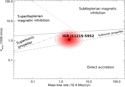
Figure 25: Left panel: position of IGR J11215-5952 (SFXT) in the $\varv_{\text{wind}}$-$\dot{M}$ diagram. Right panel: position of IGR J11215-5952 in the $\varv_{\text{wind}}$-$P_{\text{spin}}$ diagram. Equations 25, 26, 27 and 28 by Bozzo et al. (2008) are represented by a solid, dotted, triple-dot-dashed and dot-dashed lines respectively.

IGR J11215-5952 is a system with very large eccentricity and long orbital period (Romano et al. 2009). It shows recurrent flares with a period of $\sim 330$d (Sidoli et al. 2006). Its high variability leads to its classification as a SFXT, even though the predictability of the flares is not a common feature in the rest of SFXTs. Sidoli et al. (2007) proposed that the recurrent flares might be explained by an additional equatorial component of the stellar wind combined with the highly eccentric orbit. In Figure 25 we can see that a moderate clumpiness would lead to frequent transition regimes, and hence it would be expected a very high X-rays variability. However, the diagram shown in Figure 25 is calculated assuming a circular orbit, which is not accurate for IGR J11215-5952. In this source, the high eccentricity of the system might be a more important factor than the clumpiness of the wind, and the transition into the direct accretion regime might be likely only during near-periastron passages, producing periodic outbursts.

Regarding other systems, the framework used here might encounter problems to explain the behavior of other SFXTs with larger $P_{\text{spin}}$ such as IGR J16418-4532 ($P_{\text{spin}}=1212$s, Sidoli et al. 2012) and IGR J16465-4507 ($P_{\text{spin}}=228$s, Lutovinov et al. 2005). The estimation of the stellar wind parameters in these systems will be very useful to measure the extent of the applicability of the model by Bozzo et al. (2008) explaining the dichotomy between SGXBs and SFXTs. Moreover, studies of the X-rays absorption might provide an additional perspective on the issue. Giménez-García et al. (2015) studied a sample of SGXBs and SFXTs using XMM-Newton and it was observed that the SGXBs included in the sample were in general more absorbed than the SFXTs. This may suggest a more intense interaction of the X-rays radiation with the stellar wind, or, alternatively, that the neutron star orbits a more dense medium in SGXBs due to a closer orbit or a slower stellar wind of the donor.

Finally, we can compare the $\varv_{\infty}$ and the $\varv_{\text{esc}}$ that we obtain from the fits. In this regard, Lamers et al. (1995) collected a large dataset from hot stars with radiatively driven winds, and concluded that the ratio $\varv_{\infty}/\varv_{\text{esc}}$ steeply decreases from $\sim 2.6$ to $\sim 1.3$ when going from high to low $T_{\text{eff}}$ at a point near $T_{\text{eff}}\simeq 21000$ K, corresponding to spectral type around B1. According to Vink et al. (1999), this drop is caused by a decrease in the line acceleration of Fe iii in the subsonic part of the wind. In our case we have (see Table 3):

• IGR J17544-2619 (O9.5I): $\varv_{\infty}/\varv_{\text{esc}}=2.4_{-0.5}^{+0.7}$

• Vela X-1 (B0.5I): $\varv_{\infty}/\varv_{\text{esc}}=1.6_{-0.4}^{+0.8}$

These values follow the trend observed and described by Lamers et al. (1995). We suggest that it might be the reason why IGR J17544-2619 shows higher $\varv_{\infty}$ than Vela X-1. The action of the X-rays can also make an important impact in the velocity of the stellar wind, as shown by Karino (2014). However, this effect is probably local, since we do not observe important differences in the terminal velocity between eclipsing and non-eclipsing orbital phases in Vela X-1. Secondary features like asymmetries or additional absorption components in the spectral lines, which might be related to the effect of the X-rays in the stellar wind, are described and discussed below in Sect. 5.3.

5.2 Evolutionary tracks

In Fig. 22 we show the position of Vela X-1 and IGR J17544-2619 in the Hertzprung-Russell Diagram (HRD), and the evolutionary tracks from the Geneva Stellar Models (Ekström et al. 2012). The two stars lie on the theoretical track of a star with initial mass $\sim 25-30\,M_{\odot}$. In IGR J17544-2619 the spectroscopic mass obtained from the fits is compatible with the evolutionary mass. Vela X-1 shows certain overluminosity, since its spectroscopic mass is lower than the evolutionary mass. Nevertheless, the mass of the star obviously decreases along its lifetime due to the stellar wind and possible mass transfer episodes. These phenomena might have been stronger or longer in Vela X-1 compared to IGR J17544-2619.

The overabundance of helium and nitrogen arising from the fits in the two stars might trigger an increase in luminosity following the scaling relation $L\propto\mu^{\alpha}$, where $\mu$ is the average mean molecular weight and $\alpha>1$ (Langer 1992). Then, we expect certain overluminosity in both sources. However, as already mentioned, the overluminosity is more noticeable in Vela X-1. In all, the sources seem to be in a different evolutionary stage or to have experienced a different evolutionary history.

The chemical evolution of the donors might have been driven by episodes of important mass transfer in the past, given the close orbits of the systems, enhancing the helium and nitrogen abundances due to the accretion of chemically enriched material (Langer 2012). Moreover, Roche-lobe overflow stages induce important spin-up in the mass gainer (Packet 1981), inducing further chemical enrichment because of rotational mixing. This scenario is supported by the observation of other HMXBs where indications of nitrogen enhancement are also observed (González-Galán et al. 2014).

Figure 22: Evolutionary tracks from the Geneva Stellar Models with solar abundances and rotation. The positions of IGR J17544-2619 (square) and Vela X-1 (diamond) are overplotted.

5.3 Asymmetries in spectral lines of Vela X-1

Some of the lines in the spectrum of Vela X-1 show clear asymmetries that are not possible to reproduce with spherically symmetric models like PoWR (see Fig. 23). This striking feature is specially noticeable for He i lines, but it is also observed in C, N, O or Si, whenever the lines are strong enough.

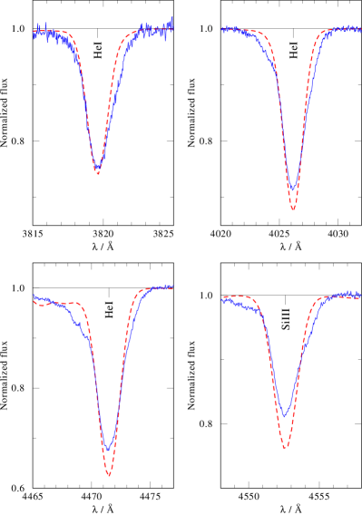
Figure 23: Example of four spectral lines showing notable asymmetries: He i $\lambda 3820,4026,4471\,\AA$, and Si iii $\lambda 4553\,\AA$.

Asymmetries in spectral lines were also reported by Martínez-Núñez et al. (2015) in hydrogen lines of the infrared spectrum of X1908+75, a SGXB. A natural explanation for the discrepancy between models and observations is the departure of the donor and/or the surrounding medium from the spherical symmetry. This departure may be triggered by tidally induced effects and the persistent X-ray irradiation of the stellar wind and the stellar surface. In this regard, Koenigsberger et al. (2012) showed that tidal effects would produce asymmetries in the line profiles.

The observed asymmetries might be related to the additional absorption that we observe in the blue part of other important lines, with special attention to H$\alpha$, H$\beta$, H$\gamma$ and Si iv $\lambda\,1394,1403\ \AA$ (see Fig. 24). Assuming that the absorption is produced by an independent component of matter moving at certain velocity, it is striking that the involved velocities required for explaining such a blueshif are different depending on the lines: $\sim 200-300$ km/s in H$\alpha$, H$\beta$ and H$\gamma$, $\sim 1000$ km/s in the Si iv resonance lines.

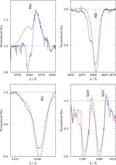
Figure 24: H$\alpha$, H$\beta$, H$\gamma$ and Si iv $\lambda 1394,1403\,\AA$. The observations (blue solid line) shows an additional blueshifted component that we are not able to reproduce with the models (red dashed line).

In any case, we note that these asymmetries and additional absorption features have not been observed in IGR J17544-2619. Hence, the physical cause at work is playing a significantly more important role in Vela X-1 than in IGR J17544-2619. This fact suggests that the interaction of the X-ray source with the stellar wind might be fundamental for understanding these asymmetries, given that the X-rays are on average more intense in Vela X-1. Indeed, if we compare the wind mechanic luminosity $L_{\text{mech}}=\dot{M}\,\varv_{\infty}^{2}/2$ to the X-ray luminosity $L_{\text{X}}$ we obtain:

• IGR J17544-2619: $L_{\text{mech}}\simeq 10^{36}$ erg/s. That is to say, at least two orders of magnitude higher than the usual X-ray luminosity of the source.

• Vela X-1: $L_{\text{mech}}\simeq 10^{35}$ erg/s. Namely, about one order of magnitude lower than the X-ray luminosity of the source in quiescence.

Hence, there is a fundamental difference in the ratio $L_{\text{mech}}/L_{\text{X}}$. The X-rays are much more powerful with respect to the stellar wind in Vela X-1 rather than in IGR J17544-2619. We suggest that this fact might be related to the asymmetries that we observe in the spectral lines of Vela X-1, but not in IGR J17544-2619.

6 Summary and conclusions

We have performed a detailed analysis of the donors of the HMXBs IGR J17544-2619 and Vela X-1, using the code PoWR that computes models of hot stellar atmospheres. We found the luminosity, extinction, stellar mass, stellar radius, effective temperature, effective surface gravity, terminal velocity of the stellar wind, mass-loss rate, clumping factor, micro and macro-turbulent velocity, rotational velocity and chemical abundances.

The estimation of the above mentioned parameters has implications on other physical parameters of the system: the derived stellar radius of IGR J17544-2619 implies an upper limit in the eccentricity of the source: $e<0.25$. The rotational velocity derived for Vela X-1 implies that the mass of the neutron star might be $M^{\text{NS}}_{\textsc{Vela\,X-1}}\sim 1.5\,M_{\odot}$, close to the canonical value ($1.4\,M_{\odot}$).

The donors of IGR J17544-2619 and Vela X-1 are similar in many of the parameters that physically characterise them and their spectrum. Moreover, they are also comparable in the eccentricity and orbital separation. However, in the context of accretion regimes described by Bozzo et al. (2008), their moderate differences in the stellar wind velocity and the $P_{\text{spin}}$ of the neutron star lead to a very different accretion regimes of the sources, which qualitatively explain their completely different X-ray behavior. After analysing other sources with sufficient information available in the literature, we have observed that the same theoretical framework is valid to qualitatively explain their X-ray behavior. Further explorations addressing the estimation of the stellar wind properties of the donors in SGXBs and SFXTs, complemented with $P_{\text{spin}}$ measurements in SFXTs, will be necessary to confirm whether the conclusions exposed here can be extrapolated to additional members of these groups of HMXBs.

In summary, this study shows that the wind terminal velocity play a decisive role in determining the class of HMXB hosting a supergiant donor. While low stellar wind velocity facilitates direct steady accretion in SGXBs, the high wind velocity and velocity jumps can easily shift the accretion mechanism from direct accretion to propeller regimes in SFXTs. This effects might be enhanced by other factors such as the eccentricity of the sources. We conclude that this is one of the mechanisms responsible for these two major sub-classes of HMXBs with supergiant donors.

Acknowledgments. The work of AG-G has been supported by the Spanish MICINN under FPI Fellowship BES-2011-050874 associated to the project AYA2010-15431. T.S. is grateful for financial support from the Leibniz Graduate School for Quantitative Spectroscopy in Astrophysics, a joint project of the Leibniz Institute for Astrophysics Potsdam (AIP) and the Institute of Physics and Astronomy of the University of Potsdam. This work has been partially supported by the Spanish Ministry of Economy and Competitiveness project numbers ESP2013-48637-C2-2P and ESP2014-53672-C3-3-P, the Generalitat Valenciana project number GV2014/088 and the Vicerectorat d’Investigació, Desenvolupament i Innovació de la Universitat d’Alacant under grant GRE12-35. We wish to thank Thomas E. Harrison for his important contribution to the paper reducing the SpeX data. We also thank S. Popov for a very useful discussion. The authors gratefully acknowledge the constructive comments on the paper given by the anonymous referee. SMN thanks the support of the Spanish Unemployment Agency, allowing her to continue her scientific collaborations during the critical situation of the Spanish Research System. The authors acknowledge the help of the International Space Science Institute at Bern, Switzerland, and the Faculty of the European Space Astronomy Centre. A.S. is supported by the Deutsche Forschungsgemeinschaft (DFG) under grant HA 1455/26. Some of the data presented in this paper were obtained from the Multimission Archive at the Space Telescope Science Institute (MAST). STScI is operated by the Association of Universities for Research in Astronomy, Inc., under NASA contract NAS5-26555. Support for MAST for non-HST data is provided by the NASA Office of Space Science via grant NAG5-7584 and by other grants and contracts. This publication makes use of data products from the Two Micron All Sky Survey, which is a joint project of the University of Massachusetts and the Infrared Processing and Analysis Center/California Institute of Technology, funded by the National Aeronautics and Space Administration and the National Science Foundation.

Appendix A Other sources

In this appendix we show the diagrams that are further discussed in Sect. 5, calculated from the available data in the literature, which is collected in Table 6.

Parameters	J11215-5952	GX 301-2	X1908+075	OAO 1657-415
	(SFXT)	(SGXB)	(SGXB)	(SGXB)
$P_{\text{orb}}$ (d)	$164.6^{a}$	$41.508^{d}$	$4.4007^{g}$	$10.44812^{i}$
$P_{\text{spin}}$ (s)	$186.78^{b}$	$685^{e}$	$604.684^{g}$	$38.2^{j}$
$M_{\star}/M_{\odot}$	$30^{c}$	$43^{e}$	$15^{h}$	$14.3^{k}$
$R_{\star}/R_{\odot}$	$40^{c}$	$70^{e}$	$16^{h}$	$24.8^{k}$
$a$ ($10^{12}$cm)	$27.2^{l}$	$11.0^{l}$	$2.4^{l}$	$4.2^{l}$
$a$ ($R_{\star}$)	$9.8$	$2.3$	$2.1$	$2.5^{l}$
$B$ ($10^{12}$G)	$1.45^{n}$	$3.8^{f}$	$1.45^{n}$	$1.45^{n}$
$\varv_{\text{wind}}$ (km/s)	$1128^{c}$	$110^{e}$	$235^{h}$	$156^{k}$
$\beta$	$0.8^{n}$	$1.75^{e}$	$1.2^{h}$	$0.9^{k}$

Table 6: Parameters used in Appendix A.
References: (a) Romano et al. (2009) (b) Swank et al. (2007) (c) Lorenzo et al. (2014) (d) Sato et al. (1986) (e) Kaper et al. (2006) (For $P_{\text{spin}}$, we used an intermediate value in the observed range $675\text{s}<P_{\text{spin}}<700\text{s}$ in the 1974-2001 period). (f) Kreykenbohm et al. (2004) (g) Levine et al. (2004) (h) Martínez-Núñez et al. (2015) (i) Barnstedt et al. (2008) (j) White & Pravdo (1979) (k) Mason et al. (2012) (l) From $P_{\text{orb}}$, total mass of the system and the 3rd Kepler’s law. (n) Not based in any estimation. Assumed as the same value as in IGR J17544-2619.

Figure 26: Left panel: position of GX 301-2 (SGXB) in the $\varv_{\text{wind}}$-$\dot{M}$ diagram. Right panel: position of GX 301-2 in the $\varv_{\text{wind}}$-$P_{\text{spin}}$ diagram. Equations 25, 26, 27 and 28 by Bozzo et al. (2008) are represented by a solid, dotted, triple-dot-dashed and dot-dashed lines respectively.

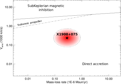
Figure 27: Left panel: position of X1908+075 (SGXB) in the $\varv_{\text{wind}}$-$\dot{M}$ diagram. Right panel: position of X1908+075 in the $\varv_{\text{wind}}$-$P_{\text{spin}}$ diagram. Equations 25, 26, 27 and 28 by Bozzo et al. (2008) are represented by a solid, dotted, triple-dot-dashed and dot-dashed lines respectively.

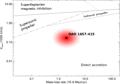
Figure 28: Left panel: position of OAO 1657-415 (SGXB) in the $\varv_{\text{wind}}$-$\dot{M}$ diagram. Right panel: position of OAO 1657-415 in the $\varv_{\text{wind}}$-$P_{\text{spin}}$ diagram. Equations 25, 26, 27 and 28 by Bozzo et al. (2008) are represented by a solid, dotted, triple-dot-dashed and dot-dashed lines respectively.

Appendix B Spectra

B.1 IGR J17544-2619

Figure 29: continued.

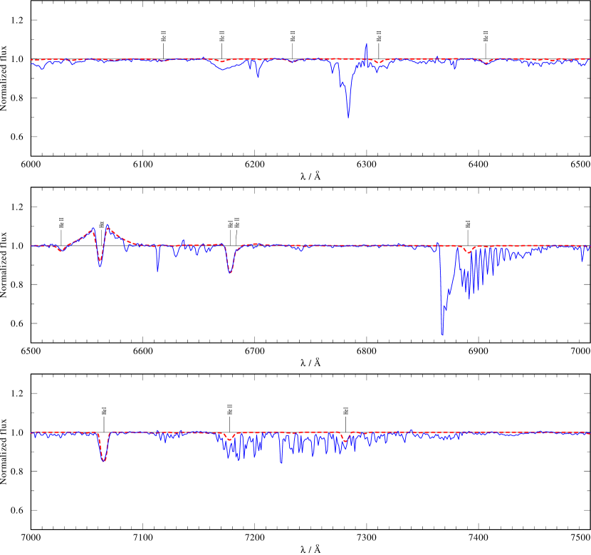
Figure 30: Optical spectrum of IGR J17544-2619 (blue), and the best fit model (red).

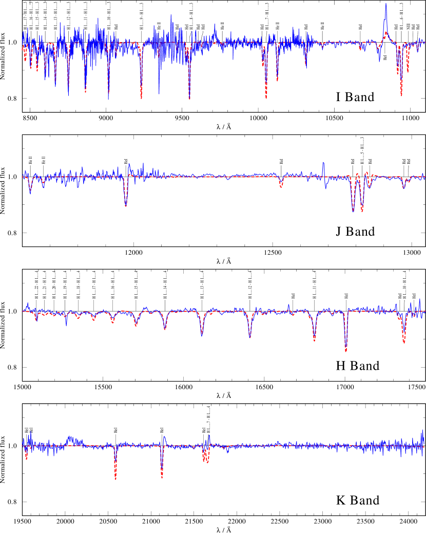
Figure 31: Infrared spectrum of IGR J17544-2619 (blue), and the best fit model (red).

B.2 Vela X-1

Figure 33: continued.

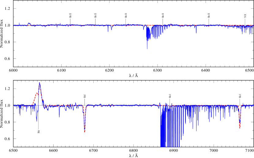
Figure 34: Optical spectrum of Vela X-1 (blue), and the best fit model (red).

References

- Asplund et al. (2009) Asplund, M., Grevesse, N., Sauval, A. J., & Scott, P. 2009, ARA&A, 47, 481
- Barnstedt et al. (2008) Barnstedt, J., Staubert, R., Santangelo, A., et al. 2008, A&A, 486, 293
- Barziv et al. (2001) Barziv, O., Kaper, L., Van Kerkwijk, M. H., Telting, J. H., & Van Paradijs, J. 2001, A&A, 377, 925
- Baum et al. (1992) Baum, E., Hamann, W.-R., Koesterke, L., & Wessolowski, U. 1992, A&A, 266, 402
- Bhalerao et al. (2015) Bhalerao, V., Romano, P., Tomsick, J., et al. 2015, MNRAS, 447, 2274
- Bildsten et al. (1997) Bildsten, L., Chakrabarty, D., Chiu, J., et al. 1997, ApJS, 113, 367
- Blondin et al. (1990) Blondin, J. M., Kallman, T. R., Fryxell, B. A., & Taam, R. E. 1990, ApJ, 356, 591
- Bondi (1952) Bondi, H. 1952, MNRAS, 112, 195
- Bozzo et al. (2008) Bozzo, E., Falanga, M., & Stella, L. 2008, ApJ, 683, 1031
- Bozzo et al. (2015) Bozzo, E., Romano, P., Ducci, L., Bernardini, F., & Falanga, M. 2015, Advances in Space Research, 55, 1255
- Cassinelli & Olson (1979) Cassinelli, J. P. & Olson, G. L. 1979, ApJ, 229, 304
- Castor et al. (1975) Castor, J. I., Abbott, D. C., & Klein, R. I. 1975, ApJ, 195, 157
- Chodil et al. (1967) Chodil, G., Mark, H., Rodrigues, R., Seward, F. D., & Swift, C. D. 1967, ApJ, 150, 57
- Clark et al. (2009) Clark, D. J., Hill, A. B., Bird, A. J., et al. 2009, MNRAS, 399, L113
- Cutri et al. (2003) Cutri, R. M., Skrutskie, M. F., van Dyk, S., et al. 2003, VizieR Online Data Catalog, 2246, 0
- Drave et al. (2014) Drave, S. P., Bird, A. J., Sidoli, L., et al. 2014, MNRAS, 439, 2175
- Drave et al. (2012) Drave, S. P., Bird, A. J., Townsend, L. J., et al. 2012, A&A, 539, A21
- Ducati (2002) Ducati, J. R. 2002, VizieR Online Data Catalog, 2237, 0
- Dupree et al. (1980) Dupree, A. K., Gursky, H., Black, J. H., et al. 1980, ApJ, 238, 969
- Ekström et al. (2012) Ekström, S., Georgy, C., Eggenberger, P., et al. 2012, A&A, 537, A146
- Elsner & Lamb (1976) Elsner, R. F. & Lamb, F. K. 1976, Nature, 262, 356
- Feldmeier et al. (1996) Feldmeier, A., Anzer, U., Boerner, G., & Nagase, F. 1996, A&A, 311, 793
- Feldmeier et al. (1997) Feldmeier, A., Puls, J., & Pauldrach, A. W. A. 1997, A&A, 322, 878
- Fitzpatrick (1999) Fitzpatrick, E. L. 1999, PASP, 111, 63
- Fraser et al. (2010) Fraser, M., Dufton, P. L., Hunter, I., & Ryans, R. S. I. 2010, MNRAS, 404, 1306
- Giménez-García et al. (2015) Giménez-García, A., Torrejón, J. M., Eikmann, W., et al. 2015, A&A, 576, A108
- González-Fernández et al. (2014) González-Fernández, C., Asensio Ramos, A., Garzón, F., Cabrera-Lavers, A., & Hammersley, P. L. 2014, ApJ, 782, 86
- González-Galán (2015) González-Galán, A. 2015, ArXiv e-prints [arXiv:1503.01087]
- González-Galán et al. (2014) González-Galán, A., Negueruela, I., Castro, N., et al. 2014, A&A, 566, A131
- Gräfener et al. (2002) Gräfener, G., Koesterke, L., & Hamann, W.-R. 2002, A&A, 387, 244
- Gray (1975) Gray, D. F. 1975, ApJ, 202, 148
- Grebenev (2010) Grebenev, S. A. 2010, ArXiv e-prints [arXiv:1004.0293]
- Grebenev & Sunyaev (2007) Grebenev, S. A. & Sunyaev, R. A. 2007, Astronomy Letters, 33, 149
- Hamann & Gräfener (2003) Hamann, W.-R. & Gräfener, G. 2003, A&A, 410, 993
- Hillier et al. (2012) Hillier, D. J., Bouret, J.-C., Lanz, T., & Busche, J. R. 2012, MNRAS, 426, 1043
- Howarth et al. (1997) Howarth, I. D., Siebert, K. W., Hussain, G. A. J., & Prinja, R. K. 1997, MNRAS, 284, 265
- in’t Zand (2005) in’t Zand, J. J. M. 2005, A&A, 441, L1
- Joss & Rappaport (1984) Joss, P. C. & Rappaport, S. A. 1984, ARA&A, 22, 537
- Kaper et al. (1994) Kaper, L., Hammerschlag-Hensberge, G., & Zuiderwijk, E. J. 1994, A&A, 289, 846
- Kaper et al. (2006) Kaper, L., van der Meer, A., & Najarro, F. 2006, A&A, 457, 595
- Karino (2014) Karino, S. 2014, PASJ, 66, 34
- Kaufer et al. (1999) Kaufer, A., Stahl, O., Tubbesing, S., et al. 1999, The Messenger, 95, 8
- Koenigsberger et al. (2012) Koenigsberger, G., Moreno, E., & Harrington, D. M. 2012, A&A, 539, A84
- Kreykenbohm et al. (2002) Kreykenbohm, I., Coburn, W., Wilms, J., et al. 2002, A&A, 395, 129
- Kreykenbohm et al. (2004) Kreykenbohm, I., Wilms, J., Coburn, W., et al. 2004, A&A, 427, 975
- Kreykenbohm et al. (2008) Kreykenbohm, I., Wilms, J., Kretschmar, P., et al. 2008, A&A, 492, 511
- Krtička et al. (2009) Krtička, J., Feldmeier, A., Oskinova, L. M., Kubát, J., & Hamann, W.-R. 2009, A&A, 508, 841
- Krtička & Kubát (2009) Krtička, J. & Kubát, J. 2009, MNRAS, 394, 2065
- Krtička et al. (2015) Krtička, J., Kubát, J., & Krtičková, I. 2015, A&A, 579, A111
- Lamers et al. (1995) Lamers, H. J. G. L. M., Snow, T. P., & Lindholm, D. M. 1995, ApJ, 455, 269
- Langer (1992) Langer, N. 1992, A&A, 265, L17
- Langer (2012) Langer, N. 2012, ARA&A, 50, 107
- Lattimer & Steiner (2014) Lattimer, J. M. & Steiner, A. W. 2014, ApJ, 784, 123
- Levine et al. (2004) Levine, A. M., Rappaport, S., Remillard, R., & Savcheva, A. 2004, ApJ, 617, 1284
- López-Corredoira et al. (2002) López-Corredoira, M., Cabrera-Lavers, A., Garzón, F., & Hammersley, P. L. 2002, A&A, 394, 883
- Lorenzo et al. (2014) Lorenzo, J., Negueruela, I., Castro, N., et al. 2014, A&A, 562, A18
- Lutovinov et al. (2005) Lutovinov, A., Revnivtsev, M., Gilfanov, M., et al. 2005, A&A, 444, 821
- Lutovinov et al. (2013) Lutovinov, A. A., Revnivtsev, M. G., Tsygankov, S. S., & Krivonos, R. A. 2013, MNRAS, 431, 327
- Manousakis & Walter (2015) Manousakis, A. & Walter, R. 2015, ArXiv e-prints [arXiv:1507.01016]
- Martínez-Núñez et al. (2015) Martínez-Núñez, S., Sander, A., Gímenez-García, A., et al. 2015, A&A, 578, A107
- Martínez-Núñez et al. (2014) Martínez-Núñez, S., Torrejón, J. M., Kühnel, M., et al. 2014, A&A, 563, A70
- Martins et al. (2005) Martins, F., Schaerer, D., & Hillier, D. J. 2005, A&A, 436, 1049
- Mason et al. (2012) Mason, A. B., Clark, J. S., Norton, A. J., et al. 2012, MNRAS, 422, 199
- Mauche et al. (2007) Mauche, C. W., Liedahl, D. A., Akiyama, S., & Plewa, T. 2007, Progress of Theoretical Physics Supplement, 169, 196
- McClintock et al. (1976) McClintock, J. E., Rappaport, S., Joss, P. C., et al. 1976, ApJ, 206, L99
- Negueruela et al. (2006) Negueruela, I., Smith, D. M., Reig, P., Chaty, S., & Torrejón, J. M. 2006, in ESA Special Publication, Vol. 604, The X-ray Universe 2005, ed. A. Wilson, 165
- Negueruela et al. (2008) Negueruela, I., Torrejón, J. M., Reig, P., Ribó, M., & Smith, D. M. 2008, in American Institute of Physics Conference Series, Vol. 1010, A Population Explosion: The Nature & Evolution of X-ray Binaries in Diverse Environments, ed. R. M. Bandyopadhyay, S. Wachter, D. Gelino, & C. R. Gelino, 252–256
- Oskinova et al. (2012) Oskinova, L. M., Feldmeier, A., & Kretschmar, P. 2012, MNRAS, 421, 2820
- Oskinova et al. (2007) Oskinova, L. M., Hamann, W.-R., & Feldmeier, A. 2007, A&A, 476, 1331
- Oskinova et al. (2011) Oskinova, L. M., Todt, H., Ignace, R., et al. 2011, MNRAS, 416, 1456
- Packet (1981) Packet, W. 1981, A&A, 102, 17
- Pellizza et al. (2006) Pellizza, L. J., Chaty, S., & Negueruela, I. 2006, A&A, 455, 653
- Puls et al. (2008) Puls, J., Vink, J. S., & Najarro, F. 2008, A&A Rev., 16, 209
- Quaintrell et al. (2003) Quaintrell, H., Norton, A. J., Ash, T. D. C., et al. 2003, A&A, 401, 313
- Rahoui & Chaty (2008) Rahoui, F. & Chaty, S. 2008, A&A, 492, 163
- Rayner et al. (2003) Rayner, J. T., Toomey, D. W., Onaka, P. M., et al. 2003, PASP, 115, 362
- Romano et al. (2015) Romano, P., Bozzo, E., Mangano, V., et al. 2015, A&A, 576, L4
- Romano et al. (2009) Romano, P., Sidoli, L., Cusumano, G., et al. 2009, ApJ, 696, 2068
- Sadakane et al. (1985) Sadakane, K., Hirata, R., Jugaku, J., et al. 1985, ApJ, 288, 284
- Sako et al. (1999) Sako, M., Liedahl, D. A., Kahn, S. M., & Paerels, F. 1999, ApJ, 525, 921
- Sander et al. (2015) Sander, A., Shenar, T., Hainich, R., et al. 2015, A&A, 577, A13
- Sato et al. (1986) Sato, N., Nagase, F., Kawai, N., et al. 1986, ApJ, 304, 241
- Sguera et al. (2005) Sguera, V., Barlow, E. J., Bird, A. J., et al. 2005, A&A, 444, 221
- Shakura et al. (2012) Shakura, N., Postnov, K., Kochetkova, A., & Hjalmarsdotter, L. 2012, MNRAS, 420, 216
- Shakura et al. (2014) Shakura, N., Postnov, K., Sidoli, L., & Paizis, A. 2014, MNRAS, 442, 2325
- Shenar et al. (2014) Shenar, T., Hamann, W.-R., & Todt, H. 2014, A&A, 562, A118
- Shenar et al. (2015) Shenar, T., Oskinova, L., Hamann, W.-R., et al. 2015, ApJ, 809, 135
- Sidoli (2011) Sidoli, L. 2011, ArXiv e-prints [arXiv:1111.5747]
- Sidoli et al. (2012) Sidoli, L., Mereghetti, S., Sguera, V., & Pizzolato, F. 2012, MNRAS, 420, 554
- Sidoli et al. (2006) Sidoli, L., Paizis, A., & Mereghetti, S. 2006, A&A, 450, L9
- Sidoli et al. (2009) Sidoli, L., Romano, P., Mangano, V., et al. 2009, ApJ, 690, 120
- Sidoli et al. (2008) Sidoli, L., Romano, P., Mangano, V., et al. 2008, ApJ, 687, 1230
- Sidoli et al. (2007) Sidoli, L., Romano, P., Mereghetti, S., et al. 2007, A&A, 476, 1307
- Simón-Díaz & Herrero (2007) Simón-Díaz, S. & Herrero, A. 2007, A&A, 468, 1063
- Sunyaev et al. (2003) Sunyaev, R. A., Grebenev, S. A., Lutovinov, A. A., et al. 2003, The Astronomer’s Telegram, 190, 1
- Swank et al. (2007) Swank, J. H., Smith, D. M., & Markwardt, C. B. 2007, The Astronomer’s Telegram, 999
- Šurlan et al. (2012) Šurlan, B., Hamann, W.-R., Kubát, J., Oskinova, L. M., & Feldmeier, A. 2012, A&A, 541, A37
- van Kerkwijk et al. (1995) van Kerkwijk, M. H., van Paradijs, J., Zuiderwijk, E. J., et al. 1995, A&A, 303, 483
- van Loon et al. (2001) van Loon, J. T., Kaper, L., & Hammerschlag-Hensberge, G. 2001, A&A, 375, 498
- Vidal et al. (1973) Vidal, N. V., Wickramasinghe, D. T., & Peterson, B. A. 1973, ApJ, 182, L77
- Vink et al. (1999) Vink, J. S., de Koter, A., & Lamers, H. J. G. L. M. 1999, A&A, 350, 181
- Walter et al. (2015) Walter, R., Lutovinov, A. A., Bozzo, E., & Tsygankov, S. S. 2015, A&A Rev., 23, 2
- Walter & Zurita Heras (2007) Walter, R. & Zurita Heras, J. 2007, A&A, 476, 335
- Watanabe et al. (2006) Watanabe, S., Sako, M., Ishida, M., et al. 2006, ApJ, 651, 421
- White & Pravdo (1979) White, N. E. & Pravdo, S. H. 1979, ApJ, 233, L121
- Zacharias et al. (2012) Zacharias, N., Finch, C. T., Girard, T. M., et al. 2012, VizieR Online Data Catalog, 1322, 0
- Zuiderwijk (1995) Zuiderwijk, E. J. 1995, A&A, 299, 79