Particle diffusion and localized acceleration in inhomogeneous AGN jets - Part II: stochastic variation

Abstract

We study the stochastic variation of blazar emission under a 2-D spatially resolved leptonic jet model we previously developed. Random events of particle acceleration and injection in small zones within the emission region are assumed to be responsible for flux variations. In addition to producing spectral energy distributions that describe the observed flux of Mrk 421, we further analyze the timing properties of the simulated light curves, such as the power spectral density (PSD) at different bands, flux-flux correlations, as well as the cross-correlation function between X-rays and TeV $\gamma$-rays. We find spectral breaks in the PSD at a timescale comparable to the dominant characteristic time scale in the system, which is usually the pre-defined decay time scale of an acceleration event. Cooling imposes a delay, and so PSDs taken at lower energy bands in each emission component (synchrotron or inverse Compton) generally break at longer timescales. The flux-flux correlation between X-rays and TeV $\gamma$-rays can be either quadratic or linear, depending on whether or not there are large variation of the injection into the particle acceleration process. When the relationship is quadratic, the TeV flares lag the X-ray flares, and the optical & GeV flares are large enough to be comparable to the ones in X-ray. When the relationship is linear, the lags are insignificant, and the optical & GeV flares are small.

1 Introduction

Blazars are a special group of Active Galactic Nuclei (AGN) whose observed radiation is dominated by relativistic jets. They show erratic variability at almost all electromagnetic wavelengths (Ulrich et al., 1997). The most extreme variations are observed in $\gamma$-rays, where amplitudes can be as large as a factor of 50 (e.g. Acciari et al., 2014), and the doubling time of the flux can be as short as 3 minutes (Aharonian et al., 2007). Variability in different wavebands is usually correlated (e.g. Fossati et al., 2008; Chatterjee et al., 2008) with notable exceptions (Krawczynski et al., 2004; Aharonian et al., 2009b). Because most of the blazar emission comes from non-thermal radiation of plasma in the relativistic jets that moves in a direction highly aligned with our line of sight, strong relativistic beaming effects alter the temporal and spectral features of the emission (Urry & Padovani, 1995), contributing to the violent variability of blazars. For example, it can shorten the timescales of the variations, and make them appear much faster than the intrinsic variation timescales in the jets’ comoving frame. But even with this considered, significant variability on the timescale of several minutes is still not readily explained for jets with sizes presumably larger than the Schwarzschild radii of the black holes (Aharonian et al., 2007). In fact, most of those extreme temporal features observed in blazars are still yet to be understood.

The rich information carried within time-series data may also provide vital clues for the discrimination of currently degenarate emission models, namely the leptonic and hadronic models of high-energy emission (Böttcher et al., 2013). The former can be further classified into synchrotron self-Compton (SSC) models (Maraschi et al., 1992) and external Compton (EC) models (Dermer et al., 1992; Ghisellini & Madau, 1996; Sikora et al., 2009), while the latter consists of proton synchrotron (Mücke & Protheroe, 2001), p-p pion production (Pohl & Schlickeiser, 2000), and p-$\gamma$ pion production (Mannheim & Biermann, 1992; Mannheim, 1993) models. Furthermore, detailed time-dependent modeling of the blazar jets can help constrain the physical conditions such as emission location, magnetic field, size, and even composition of the jets (Petropoulou, 2014; Diltz et al., 2015; Sokolov et al., 2004; Zacharias & Schlickeiser, 2013).

Time-dependent modeling of blazars usually refers to well defined, ’clean’ flares (Saito et al., 2015; Chen et al., 2011; Zhang et al., 2015), because only in those cases can one easily identify a single physical event that may possibly reproduce the observation. However, there is no guarantee that such clean flares are representative of the general behavior of blazar variability. In fact, clean flares with predictable raising and decaying phases are relatively rare (Nalewajko, 2013). Most of the light curve may be better described as a succession of flares that overlap each other, if one insists on describing light curves with flares (Aharonian et al., 2007; Abdo et al., 2010b). An alternative approach is to continuously change one or more parameters in the model so that the resulting light curves match an entire observation campaign in at least one waveband (Krawczynski et al., 2002). This approach keeps the modeling close to observation and provides a good way to probe the underlying physical connection between the variations at different wavebands. However, it does not offer any physical reasoning why the physical parameters change in the way the fitting process requires them, as the timing information contained in the primarily fitted wavelength is largely left unexplored.

The noise-like appearance of blazar light curves triggered interests in their power spectral density (PSD), which can reveal the distribution of flux variability on different timescales (e.g. Chatterjee et al., 2008; Abdo et al., 2010a). Studies show that blazar PSDs typically exhibit a featureless power-law spectrum close to an $1/f^{2}$ red-noise profile. However, the range of timescales covered in those studies is usually limited, because it is naturally difficult to collect time-series data over vastly different timescales. Therefore it is entirely possible that there are PSD spectral breaks that can not yet be robustly identified from the currently available data. For example, Kataoka et al. (2001) analyzed the 0.5-10 keV X-ray variability of Mrk 421, and the results suggested a break of the PSD indices around $10^{-5}$ Hz, close to the longest time scale accessible with their data. A more recent analysis of 3-10 keV X-ray variability on longer time scales (Isobe et al., 2015) confirms a relatively soft PSD index of 1.6, although that is much harder than predicted by Kataoka et al. (2001).

The randomness in the blazar behavior prompted attempts to treat the blazar physics as stochastic processes, either using the internal shock models (Spada et al., 2001; Guetta et al., 2004; Rachen et al., 2010) or turbulence (Marscher, 2014) to explain blazar variability. With these approaches, it is practically impossible to match observed and simulated light curves, because the variation of the simulated flux at any particular time is random. However, the fluctuations obey certain probability distributions, so that over a long time, the light curves would produce predictable PSDs. Those PSDs, as simulation products, can be directly compared with the PSDs obtained from past or future observations. Additionally, the correlation between different wavebands remains very informative of the inherent physical processes. The traditional fitting of blazar spectral energy distributions (SEDs) will also be available just as in steady-state or time-dependent approaches. Combining all this information, one can take advantage of the large amount of multiwavelength data available and place strong constraints on blazar models.

In Chen et al. (2015) (Paper I hereafter), we have built an inhomogeneous jet-emission model. As an initial step towards a more comprehensive model, we studied the spectral properties of the system as it relaxes to its steady state. In this work we will expand that model by introducing stochastic processes, building time-dependent SEDs and simulating light curves to be compared with observations. The aim is to identify distinctive timing features, that can be used to explain observed variability and guide future observation or data analysis.

In this paper, all quantities in the comoving frame of the jet are primed, while quantities in the observer’s frame are unprimed. Notice that this is contrary to the convention in Paper I, because in that work most of the discussions are focused on particle processes in the comoving frame, while in this work the focus is shifted to observational consequences.

2 Stochastic Processes and PSDs

The PSD of evenly spaced time-series data can be calculated conveniently. For the ease of comparison with observations, we use the formula of Uttley et al. (2002) and Chatterjee et al. (2008) to calculate PSDs from observational light curves of blazars. First, the average flux is subtracted off all flux points in a light curve, yielding

$$\begin{split}f(t_{i})&=F(t_{i})-\frac{1}{N}\,\sum\limits_{j=1}^{N}F(t_{j})\\ &=F(t_{i})-\mu\ .\end{split}$$ (1)

The power spectral density then is

$$P(\nu)=\frac{2T}{\mu^{2}N^{2}}|F_{N}(\nu)|^{2}\ ,$$ (2)

where

$$|F_{N}(\nu)|^{2}=|\sum\limits_{i=1}^{N}f(t_{i})\mathrm{exp}(i2\pi\nu t_{i})|^{2}.$$ (3)

Here, T is the total duration of the light curves considered, N is the total number of data points, and $\mu$ is the average flux subtracted. Eq. 3 calculates the square of the modulus of the discrete Fourier transform for the light curves at linearly evenly sampled frequencies $i/T$, where $i$ are integers between 1 and $N/2$. Eq. 2 gives the fractional rms-squared normalization to the final PSD.

With the fractional rms-squared normalization used in Eq. 2, the PSDs have the property that the integral of the PSDs give the total fractional rms variability of the light curve. They give a direct view of how variable the emission is at different time scales. Of special interest are the slopes of the PSDs, which may reveal key properties of the underlying stochastic process.

In the context of discrete time series, white noise results from perhaps the most simple stochastic process. It consists of a sequence of random variables that are independent of each other. The PSD of white noise has slope zero, i.e. the power per unit frequency is uniformly distributed on all time scales.

If the signal from one time step persist to the next time step, and the random variable is allowed to accumulate, then the resulting time series becomes red noise. This stochastic process is a random walk process. The continous-time limit of a Gaussian random walk in one-dimension is called the Wiener process, which also produces red noise. The PSD of red noise has slope -2, with more variabiliy power per unit frequency distributed at large time scales.

Some further modification of the Wiener process can also allow for breaks in the slope of PSDs. One such modified process is the Ornstein-Uhlenbeck (O-U) process. It allows the accumulated signal in the Wiener process to exponentially decrease with time, on time scale $\tau$, e.g. imposed by particles escape/cooling or turbulence decay. This decrease means that at the extreme of large time scales, the earlier signal almost vanishes (acceleration events decay), and the signal approaches white noise; at the extreme of small time scales, the signal does not have enough time to decrease (acceleration events accumulate), and the process approaches a Wiener process. The PSD slope changes from 0 at large time scale to -2 at small time scale. The slope breaks approximately at frequency $1/(2\pi\tau)$. An analytical expression for the PSD of an O-U process exists (Kelly et al., 2009):

$$P(\nu)=\frac{2\sigma^{2}\tau^{2}}{1+(2\pi\tau\nu)^{2}}\ .$$ (4)

Here $\sigma$ is related to the strength of the O-U process, and is only relevant to the normalization of the PSD. For a mathematical description of the O-U process, we refer the readers to Gillespie (1996).

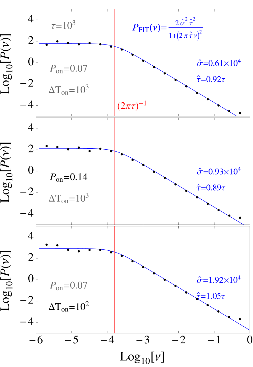
Figure 1: PSD of a stochastic process similar to the O-U process. The black dots are simulation results, while the black legends are input parameters. The blue lines are fitting to the black dots with the equation in blue. The blue parameters are results of the fitting. The vertical red line shows the frequency where we expect to see a PSD break in an O-U process. Compared to the top panel, the middle panel has a different $\Delta T_{\mathrm{on}}$, while the bottom panel has a different $P_{\mathrm{on}}$.

As a mathematical model that motivates the implementation of stochastic variations in our jet model, we simulate a slightly modified version of the O-U process where instead of Gaussian distribution, the increment follows the Bernoulli distribution, i.e. it takes value of 1 with probability $P_{\mathrm{on}}$, and takes 0 otherwise. The increment is only active on certain time steps with separation of $\Delta T_{\mathrm{on}}$, which is, for example, $10^{3}\Delta t$. Here $\Delta t$ is the time step, as well as the unit of time in these simulations. There is no extra input, i.e. the increment remains 0, on other time steps. The simulations last 6000 time steps each.

The simulated time sequence is used to produce PSDs according to eq. 1-3. The resulting $\sim 10^{6}$ PSD points are grouped into 19 bins, where the bins have the same width on the logarithmic scale in the frequency axis (x-axis of the plot). The points shown in Figure 1 represent the average values from each bin. Three plots are shown in a column to illustrate the effects of changing the increments separation, $\Delta T_{\mathrm{on}}$, and the success probability, $P_{\mathrm{on}}$.

We can see that in all these plots, above the frequency defined by $1/(2\pi\tau)$, the PSDs are compatible with red noise, whereas below the break frequency they are consistent with white noise. This is the expected characteristic of the O-U process. We fit eq. 4 to the simulated PSDs by allowing both parameters $\sigma$ and $\tau$ to vary. In practice, the logarithm of $P(\nu)$ is used for the fitting to avoid dominance of the high-power points at low frequency.

Also shown in Figure 1 is that the fitted $\hat{\tau}$ is always very close to the actual $\tau$ in the model. This shows that the break in the PSD is solely determined by the decay time scale, while not being affected by the parameters $\Delta T_{\mathrm{on}}$ or $P_{\mathrm{on}}$, as shown in the middle and bottom panels of Fig.1.

3 Model Setup

The model used in this work is built upon the spatially resolved treatment of particle acceleration and diffusion in jets that is presented in Paper I, where the discussion focused on the steady-state spectrum. The particle transport equation used in the model reads as

$$\begin{split}\frac{\partial n^{\prime}(\gamma^{\prime},\mathbf{r^{\prime}},t^{\prime})}{\partial t^{\prime}}&=-\frac{\partial}{\partial\gamma^{\prime}}\bigg{[}\dot{\gamma^{\prime}}(\gamma^{\prime},\mathbf{r^{\prime}},t^{\prime})n^{\prime}(\gamma^{\prime},\mathbf{r^{\prime}},t^{\prime})\bigg{]}\\ &+\frac{\partial}{\partial\gamma^{\prime}}\bigg{[}D^{\prime}(\gamma^{\prime},\mathbf{r^{\prime}},t^{\prime})\frac{\partial n^{\prime}(\gamma^{\prime},\mathbf{r^{\prime}},t^{\prime})}{\partial\gamma^{\prime}}\bigg{]}\\ &+\mathbf{\nabla}\cdot\bigg{[}D^{\prime}_{x}(\gamma^{\prime})\nabla n^{\prime}(\gamma^{\prime},\mathbf{r^{\prime}},t^{\prime})\bigg{]}+Q^{\prime}(\gamma^{\prime},\mathbf{r^{\prime}},t^{\prime}),\end{split}$$ (5)

where $n^{\prime}(\gamma^{\prime},\mathbf{r^{\prime}},t^{\prime})$ is the differential number density of particles, $\dot{\gamma^{\prime}}(\gamma^{\prime},\mathbf{r^{\prime}},t^{\prime})$ is the acceleration rate ( including the synchrotron and SSC cooling, which are negative), $D^{\prime}(\gamma^{\prime},\mathbf{r^{\prime}},t^{\prime})$ is the momentum diffusion coefficient, $D^{\prime}_{x}(\gamma^{\prime})$ is the spatial diffusion coefficient, and $Q^{\prime}(\gamma^{\prime},\mathbf{r^{\prime}},t^{\prime})$ is the particle injection rate. Further explanation of this equation, along with a schematic figure for the geometry can be found in Paper I. A more detailed description of the Monte Carlo/Fokker-Planck (MCFP) code used for building the model can be found in Chen et al. (2011). In the current work we adopt the Dirichlet boundary conditions ($n^{\prime}_{\mathrm{boundary}}=0$), i.e. the spatial diffusion will lead to particle escape through the outer boundary of the simulation box. The Monte-Carlo photons in the simulation output are binned according to the angle of their traveling direction to the jet axis, $\theta^{\prime}$. In order to get sufficient number of Monte Carlo photons for the bin that has Doppler factor $\delta\sim\Gamma$, we sample a finite range of $\theta^{\prime}$ around $90^{\circ}$ in the jet frame ($-0.12\leq\mathrm{cos}\theta^{\prime}\leq 0.12$ here). But the relativistic beaming is performed using the average angle (cos$\theta^{\prime}=0$) to avoid any spread in the Doppler factor for the beaming, which can cause significant spread of the flux in time when the simulation becomes relatively long. The cylindrical simulation box is divided into axisymmetrical ring-like cells in radial and vertical directions. The number of cells is nz$\times$nr=20$\times$15=300. The magnetic field is assumed to be homogeneous and disordered, so that the spatial diffusion is also isotropic. The radiation mechanism is assumed to be leptonic, with current discussions limited to SSC models, even though our MCFP code also allows for the study of EC models (Chen et al., 2012). The simulated results (§ 4) including SEDs, light curves and flux-flux correlations are plotted together with the observations of Mrk 421, the stereotypical high-energy-peak blazar that we try to compare our simulations with. This matching to Mrk 421 also influences our discussions, many of which, especially the energy bands, may appear to be specific to Mrk 421. However, most of the results are indeed applicable to other blazars, especially other high synchrotron peak blazars. The key parameters used in the benchmark case (§ 4.1) are listed in Table 1.

Table 1: The parameters used for the benchmark case in §4.1. The observation angle in the observer’s frame is always $1/\Gamma$ so that the Doppler factor $\delta$ is equal to the bulk Lorentz factor $\Gamma$. The volume height $Z^{\prime}=4R^{\prime}/3$ in all cases. Here $n^{\prime}_{\mathrm{e}}$ is the time average of the particle density of the entire region for $t^{\prime}/\Gamma>100$ ks, while $t^{\prime}_{\mathrm{acc}}$ and $Q^{\prime}_{\mathrm{inj}}$ represent the fastest acceleration time and the associated injection rate in a single cell during the simulation.

$B^{\prime}$	$Z^{\prime}$	$\delta$	$D^{\prime}_{\mathrm{x}}$	$n_{\mathrm{e}}^{\prime}$	$t^{\prime}_{\mathrm{acc}}$	$Q^{\prime}_{\mathrm{inj}}$	$\tau^{\prime}_{\mathrm{decay}}$
0.27	$10^{16}$	33	3.75	1.53	0.18	$0.020$	2
Gauss	cm	-	$\mathrm{cm}^{2}\mathrm{s}^{-1}$	$\mathrm{cm}^{-3}$	$Z^{\prime}/c$	$\mathrm{cm}^{-2}\mathrm{s}^{-1}$	$Z^{\prime}/c$

In order to achieve a stochastic increase of localized acceleration, which we use to describe the turbulent nature of the plasma, we set the acceleration rate in each cell in a way similar to the stochastic process we simulated in §2. The specific implementations of the O-U-process-like acceleration in our jet-model is as follows: In most parts of the emission region, the particles are assumed to only diffuse spatially and cool radiatively, i.e. there is no acceleration. This assumption is broken in a spinal region along the axis of the axisymmetrical jet (where the radius $r^{\prime}<10^{15}$cm), where second-order Fermi acceleration with acceleration rate $\dot{\gamma}^{\prime}_{D}(\gamma^{\prime},\mathbf{r^{\prime}},t^{\prime})=\gamma^{\prime}/t^{\prime}_{\mathrm{acc}}$ is at work. Initially, the acceleration time, $t^{\prime}_{\mathrm{acc}}$, is very long. Within this region, for every time step ($\delta t^{\prime}=\delta z^{\prime}/c=1.7\times 10^{4}\,\mathrm{s}$ here), each sub-region with 2x2 cells may experience with a probability of $P_{\mathrm{acc}}$ (=0.07 here) an increase in the acceleration rate. The increment in acceleration rate is

$$\Delta\dot{\gamma}^{\prime}_{D}=\gamma^{\prime}\,\frac{c}{2.2\,Z^{\prime}}=\gamma^{\prime}\,\frac{1}{7.3\cdot 10^{5}\ \mathrm{s}}\ .$$ (6)

These increase can happen repeatedly on the same cells. Sub-regions can overlap with each other in the z direction, so that each cell belongs to two sub-regions and has two chances of receiving additional acceleration every time step. On the other hand, the acceleration rates also decrease exponentially on the time scale $\tau^{\prime}_{\mathrm{decay}}$ all the time, everywhere. The stochastic increase of the acceleration represents additional turbulence caused by, e.g., magnetic reconnection, or other plasma processes that are inherently stochastic. The deterministic decrease on the other hand represents the dissipation of these magnetic turbulence through reconnection.

Most of the specific parameter values used in this section are tuned so that the simulated and observed SED and light curves look reasonably similar. However, as demonstrated in the previous section, the choice of the parameters like time-step and $P_{\mathrm{acc}}$ does not affect key features such as the power-law breaks in the PSDs.

One important complication in our model is that here the random variable is the acceleration rate, rather than the radiative flux that is measured directly. Because of this, several time scales besides the acceleration decay time scale become potentially relevant in the problem. Those include the radiative-cooling time scale and light-crossing time scale. We will further compare our simulation results with the O-U process, and discuss the relevance of different time scales in § 4 & 5.

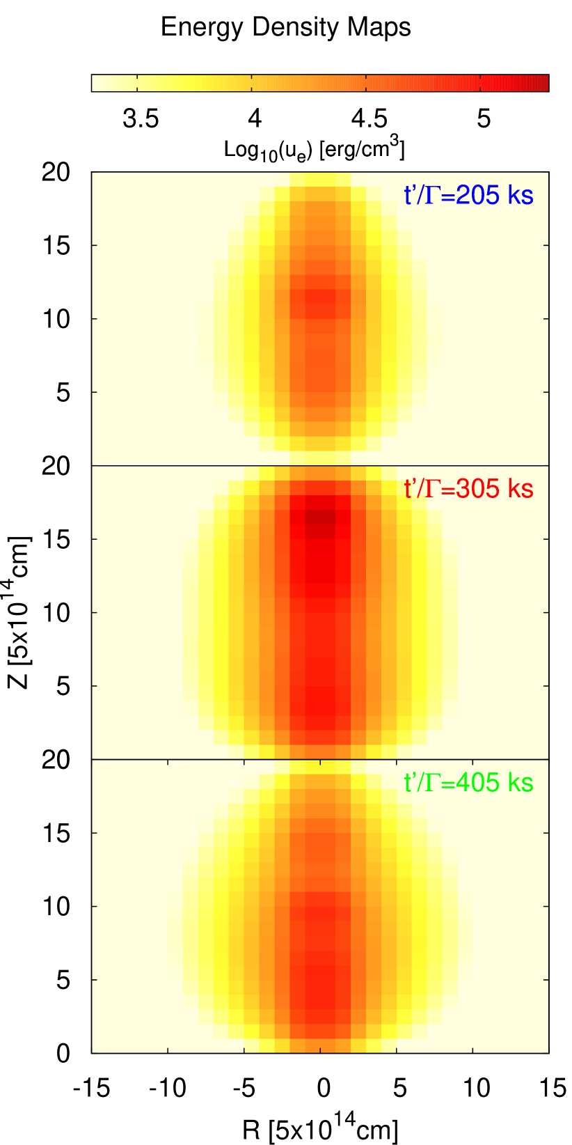
Figure 2: Three sample electron energy density maps at different time epochs from the benchmark simulation case described in § 4.1 (Case 1). $t^{\prime}/\Gamma$ are shown as rough estimates for their corresponding time in the observer’s frame, because proper relativistic beaming is not defined for electrons.

In the acceleration regions, electrons are also injected at relatively low, but still highly relativistic energy. Instead of following a Gaussian distribution as assumed in Paper I, these electrons follow the Maxwell-Jüttner distribution (Wienke, 1975; Jüttner, 1911) expressed as a function of Lorentz factor $\gamma^{\prime}$:

$$f(\gamma^{\prime})=\frac{\gamma^{\prime 2}\beta^{\prime}}{\Theta^{\prime}K_{2}(1/\Theta^{\prime})}e^{-\gamma^{\prime}/\Theta^{\prime}},$$ (7)

where $K_{2}$ is a modified Bessel function of the second kind, $\Theta^{\prime}$ is associated to the temperature $T$ as $\Theta^{\prime}=kT^{\prime}/mc^{2}$, $k$ is Boltzmann’s constant, $m$ is the rest mass of the particle (electron here), $\beta^{\prime}=v^{\prime}/c$, and c is the speed of light. $\Theta^{\prime}$ is chosen to equal the bulk Lorentz factor of the jet $\Gamma$, because the injected electrons are postulated as a result of particles in the interstellar medium being trapped and isotropized by the magnetic turbulence which also causes the particle acceleration in the jet. This is similar to the isotropization of particles of the interstellar medium through blast waves as proposed by Pohl & Schlickeiser (2000).

An illustrative example of the 2-D energy-density maps of electrons in the simulation (Case 1) is plotted in Fig. 2. The corresponding electron energy distributions averaged over the entire emission region are plotted in Fig. 3. Both figures use quantities in the co-moving jet frame. To be noted from the figures are the asymmetry in the spatial distribution of electrons and the spectral impact of the stochasticity in acceleration efficiency.

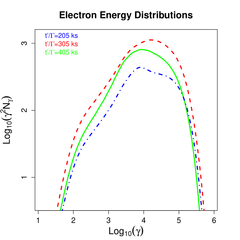
Figure 3: Three sample electron energy distributions from the benchmark case (Case 1). The time sequence is blue dot-dashed line, red dashed line, then green solid line. $t^{\prime}/\Gamma$ are shown as rough estimates for their corresponding time in the observer’s frame.

Microphysical processes that provide an enhanced level of turbulence, and hence stronger stochastic acceleration, often go along with preacceleration of particles that subsequently undergo Fermi-type acceleration. To avoid specifying the origin of fast stochastic acceleration, we investigate two representative scenarios. In the benchmark case, shown in § 4.1, the rate of particle injection at low energy, non-zero only in the acceleration region, is exponentially coupled to the acceleration rate according to

$$Q^{\prime}_{\mathrm{inj}}=Q^{\prime}_{0}\mathrm{exp}(t^{\prime}_{0}/t^{\prime}_{\mathrm{acc}}),$$ (8)

where $Q^{\prime}_{0}=10^{-7}\ \mathrm{cm}^{-2}\,\mathrm{s}^{-1}$ and $t^{\prime}_{0}=2.16\,Z^{\prime}/c$. These values are tuned so that the changes in both acceleration and injection affect the evolution of the light curves. The motivation for the exponential coupling used here is: Suppose the injection is linearly associated with the high-energy tail of a background particle population, which falls off exponentially; and suppose the pre-acceleration of the background particles is linearly associated with the localized acceleration. The injection is then exponentially associated with the peak energy of the background particles, and so is the acceleration rate. Table 1 lists the fastest injection rate we observed in the simulation.

The connection between injection and acceleration is changed in the second case (§ 4.2, representing the alternative scenario), where injection is absent where the acceleration is slow ($t^{\prime}_{\mathrm{acc}}\gg Z^{\prime}/c$). When the acceleration rate is reasonably strong ($t^{\prime}_{\mathrm{acc}}\sim Z^{\prime}/c$ or $t^{\prime}_{\mathrm{acc}}<Z^{\prime}/c$), the injection rate is set to a constant ($Q^{\prime}_{\mathrm{inj}}=4\times 10^{-3}\ \mathrm{cm}^{-2}\,\mathrm{s}^{-1}$). Effectively, this leads to a constant particle density of $1.49\ \mathrm{cm}^{-3}$.

Under the same physical scenario as the one in the benchmark case, we investigate a third case, as outlined in § 4.3. This case explores the effects of the acceleration decay rate, by changing $\tau^{\prime}_{\mathrm{decay}}$ from $2Z/c$ to $4Z/c$. To ensure the maximum acceleration rate achieved is more or less unchanged, we accordingly reduce in amplitude the stochastic increments of the acceleration.

Most simulations (except the duplicate simulation for Fig.  6) in this work use the same sequence of random numbers for the stochastic change of the acceleration rate (but not for the Monte Carlo radiative transfer). This is evident from the similar light curves seen in all cases. This makes the comparison between different cases easier, and leaves the intended change of condition in the system as the most likely cause for any differences.

4 Results

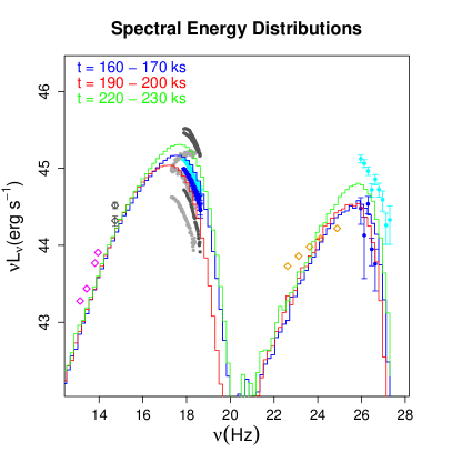
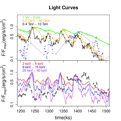
Figure 4: Left: Simulated SED (histogram) at three different time epochs for our benchmark case (Case 1). The data points include a $\gamma$-ray flare of March 19, 2001, observed by Whipple, and the simultaneous X-ray data from RossiXTE (pre-flare in blue, flare peak in cyan). X-ray and optical high/low states data taken by RossiXTE and Mt Hopkins 48-inch telescope in 2001 (dark gray), and X-ray high/low states data from BeppoSAX in 1998 and 2000 (light gray) are also shown (Fossati et al., 2008). In other bands there are WISE infrared data from May 21, 2010 in magenta, and Fermi 4-year average $\gamma$-ray data (Acero et al., 2015) in yellow. Right: Samples of normalized simulated light curves in 6 different frequency bands. Observational light curves are plotted as connected dots. They include simultaneous 2-4 keV RossiXTE X-ray (grey) and TeV Whipple/HEGRA $\gamma$-ray (dark blue) data. The time stamp 100 ks in the figure corresponds to MJD 59186.9 or March 18, 2001.

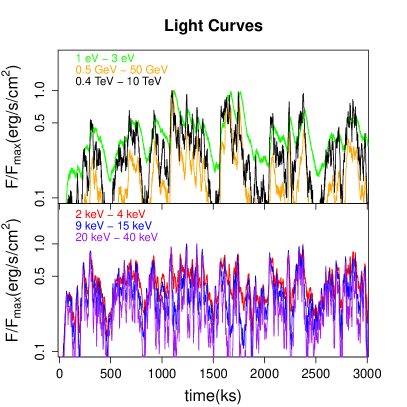
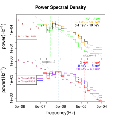
Figure 5: Left: Full light curves for the entire simulation Case 1. Right: PSD based on the light curves excluding the first 100 ks. The vertical lines indicate various timescales in the system (times $2\pi$), namely acceleration decay as blue dashed line, light crossing as blue dot-dashed line, and a red/green long dashed lines representing synchrotron cooling for electrons that emit synchrotron radiation primarily in 2-keV X-ray/ 1-eV optical band. The gray dashed line indicates a power-law with index of -2. We also plot the observational PSDs of Mrk 421. They include X-ray data from MAXI (squares) and ASCA (circle) as maroon points in the lower panel (Isobe et al., 2015) and GeV $\gamma$-ray from Fermi as brown points in the upper panel.

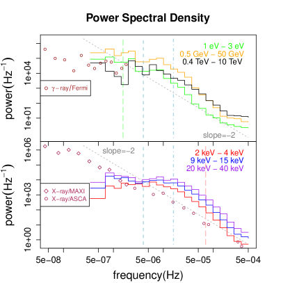
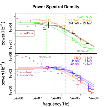
Figure 6: Left: Power spectral density for a simulation almost the same as Case 1, except a different realization of the random numbers. Right: Average PSD of the two simulations. Lines that show the O-U process fits to the PSD are plotted with matching colors. The straight comparison lines are the same as those in Fig. 5.

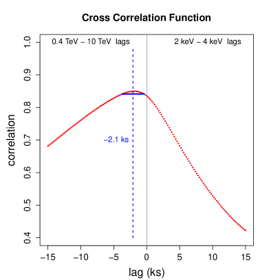
Figure 7: Correlation analysis for Case 1. Left: Flux-flux correlation between the X-ray and $\gamma$-ray bands during the time period 1200ks-1500ks. The first 30 ks are plotted in red, and the last 30 ks are plotted in cyan. The grey connected circles are observational data points for Mrk 421 on March 19, 2001 from Fossati et al. (2008). Three grey dashed lines are also plotted so that the readers can compare them to the trend of the flux-flux relationship. Right: Cross-correlation between X-ray and TeV $\gamma$-ray fluxes based on the light curves, excluding the first 100 ks. The confidence interval for the lag based on the correlation function is marked with the horizontal solid blue line, while the estimated lag is identified with the dashed blue vertical line.

Since we have multiple cases, each with a similar set of analyses that would be better understood when compared with each other, we merely list the findings of each case and the variability analysis methods in this section, and leave the interpretation of these findings to §5. The SEDs and light curves are not the focus of our study in this work. The simulated observational SEDs and light curves for each case are shown here to verify that we are using model parameters that are generally consistent with what we know about Mrk 421.

4.1 Case 1: Injection associated with acceleration

This is the benchmark simulation case for our study. The SED and light curve samples are shown in Fig 4. The conversion between apparent luminosity and flux is performed for 135 Mpc as the luminosity distance of Mrk 421. Since the results are under the influence of stochastic fluctuations, we only aim to approximately match the simulated SEDs with the observation. Likewise, the simulated and observational light curves cannot be identical. They are shown to demonstrate that they generally have similar shapes and amplitudes. The first 100 ks of the simulated light curves include the initial build up of the photon field and the stabilization of the electron energy distribution. We do not consider this period in subsequent analysis to avoid any unwanted effects from the initial condition.

4.1.1 Power Spectral Density

In our simulations, the total duration T of equation 2 is 3000 ks minus the first 100 ks, which is considered the setup phase of the simulations. The PSD points are further binned into 20 logarithmically evenly spaced frequency bins from $8.8\times 10^{-7}$ Hz to $5.9\times 10^{-4}$ Hz. The first two points are exempt from binning because of the sparseness of points at those frequencies, making 22 the total number of final PSD points for each energy.

The resulting PSD for the entire simulation (excluding the first 100 ks) is shown in Fig.5 together with the full light curves. The PSDs therefore show that the high-energy X-ray flux is most variable within the synchrotron component. Within the inverse Compton (IC) component at higher energy, the GeV $\gamma$-ray and TeV $\gamma$-ray have similar level of variability.

Table 2: Relaxation time $\tau_{\mathrm{relax}}$ in ks for various energy bands, obtained by fitting the PSDs with equation 4.

Energy	Case 1	Case 2	Case 3
1-3 eV	115	54	70
0.5-50 GeV	64	36	68
0.4-10 TeV	27	24	52
2-4 keV	21	23	48
9-15 keV	14	18	28
20-40 keV	12	15	20

The PSDs follow a broken power-law distribution, which is expected from O-U processes. However, the non-smoothness of the PSDs at low frequency indicates considerable uncertainty. This might hamper our identification of the breaks. In order to increase the reliability of the PSDs, we repeated the simulation leading to Fig. 5 with a different sequence of random numbers. The PSD of this separate simulation is shown in the left panel of Fig. 6. An average of the PSDs from the two simulations is shown in the right panel of Fig. 6.

Apart from the red/white noise above/below the break frequency, the PSDs also flatten to white noise at the highest frequencies. This is a natural result of the uncertainty in the Monte Carlo method used for the radiative transfer, which renders unreliable variability below certain threshold. This is also a great example that shows how the PSD can be used to identify at which time scales and amplitudes the variability in a light curve should be suspected of containing mostly noise.

We fit the average PSDs of the two simulations with equation 4. Only frequencies below $10^{-4}$ Hz are considered in the fitting, in order to avoid the white noise at low variation power caused by Monte-Carlo fluctuation. The best-fit relaxation times, $\tau_{\mathrm{relax}}$, are listed in Table 2. We can see that for both the synchrotron and IC emission, $\tau_{\mathrm{relax}}$ becomes smaller with increasing photon energy. For the X-ray synchrotron bands, $\tau_{\mathrm{relax}}$ is close to both the acceleration decay time, $\tau^{\prime}_{\mathrm{decay}}/\Gamma=20$ ks, and the light crossing time, $\tau^{\prime}_{\mathrm{cross}}/\Gamma=10$ ks.

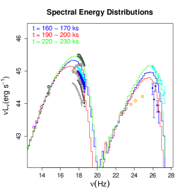
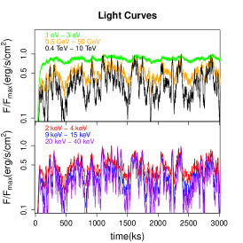
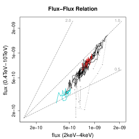
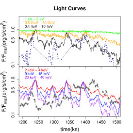
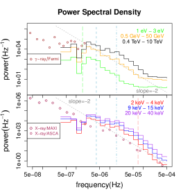
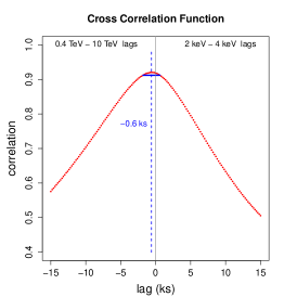
Figure 8: Figures similar to those shown in Fig. 4, 5 & 7, but for Case 2 with fixed particle injection rate (§ 4.2). Figures include SEDs, full light curves, flux-flux correlation in the top panel, as well as short light curves, PSDs, cross-correlation in the bottom panel.

4.1.2 X-ray/$\gamma$-ray Correlation

We show the flux-flux amplitude correlation and the cross-correlation function for the benchmark case in Fig. 7.

In order to obtain the uncertainty of the cross-correlation, we resample one of the two light curves without replacement, i.e. the time series of the light curve is reshuffled randomly. Then we calculate the correlation value of this reshuffled light curve with the other light curve, with zero lag. Since now the two light curves should be completely uncorrelated, the expected correlation is zero. Any non-zero values are assumed to be caused by random fluctuations around zero. By repeating this process for 2000 times, we get 2000 different cross-correlation values. The standard deviation, $\sigma_{\mathrm{cc}}$, for those 2000 values is taken as the uncertainty of the correlation. We use the maximum of the correlation in Fig. 7 minus $\sigma_{\mathrm{cc}}$ to set the confidence interval for the lag based on the correlation function, while the estimated time lag is the mid-point of this interval. For the purpose of maximizing the precision of the lags detected, we use 0.2-ks time bins instead of the 1-ks bins used in the other plots. This choice still makes sure that at all wavebands the number of Monte Carlo photons in most bins is larger than 100.

In this case the amplitudes of X-ray and TeV flux show a quadratic relationship very similar to the observed relationship in Mrk 421. The cross correlation suggests that TeV $\gamma$-ray variability lags that in X-rays by 2.1 ks.

4.2 Case 2: Fixed injection rate

In this case particle injection is constant in the acceleration region along the spine of the cylinder. Plots in format similar to those shown in Fig. 4,5 & 7 are shown in Fig. 8. The fitted parameters for the PSDs are shown in Table 2. We can see that the PSDs in this case show similar trends as the ones observed in Case 1, but compared to that case, the X-ray PSDs here generally break at longer time scales, or lower frequency, while the optical and $\gamma$-ray PSDs break at shorter time scales, or higher frequency. Another difference is that TeV $\gamma$-ray lightcurve shows a significantly higher fractional variability than that of GeV $\gamma$-rays. The flux-flux correlation is shown to be close to linear rather than quadratic. The cross-correlation function shows a small TeV $\gamma$-ray lag of 0.6 ks, that is statistically compatible with zero lag.

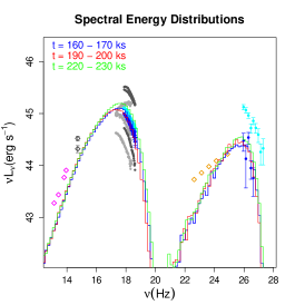
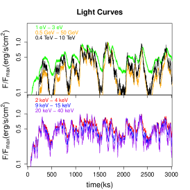
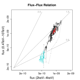
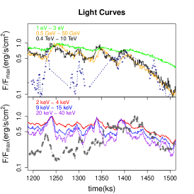
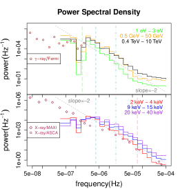
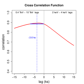
Figure 9: Figures similar to those shown in Fig. 4, 5 & 7, but for Case 3 with slower acceleration decay (§ 4.3). Figures include SEDs, full light curves, flux-flux correlation in the top panel, as well as short light curves, PSDs, cross-correlation in the bottom panel.

4.3 Case 3: Slower acceleration decay

Compared to Case 1, here the acceleration decay time scale, $\tau^{\prime}_{\mathrm{decay}}$, is changed from $2Z^{\prime}/c$ to $4Z^{\prime}/c$. The results are shown in Fig. 9. Mostly they are consistent with the results of Case 1. The effect of the longer acceleration decay time is that most of the fitted relaxation times $\tau_{\mathrm{relax}}$ (except optical) for the PSDs become roughly a factor of 2 larger, which is a result of doubling of the acceleration decay time. The complication with the optical PSD is that, based on the $\tau_{\mathrm{relax}}$ obtained in Case 1, the one expected from the current case should be about 230 ks, which puts $1/2\pi\tau_{\mathrm{relax}}\sim 7\times 10^{-7}$Hz close to the edge of the covered frequency. This means the frequency range we use might not be sufficient to accurately identify the PSD break of optical emission in this case. Therefore the value obtained here should be treated with caution.

5 Discussion

5.1 Comparison with Observation

In all the simulated cases, there is a good match between the simulated and observational SED, except the spectral indices at $\gamma$-rays. The SED observed by Fermi appears to be softer, which is at least partially caused by the fact that the Fermi data points are 4-year averages, while the other points and the simulation are snapshot SEDs at flaring state. The SED at very high energy (VHE) $\gamma$-rays ($\gamma$-rays above 300 GeV) is also always slightly softer than the observed one (see also Fossati et al., 2008) . This softer $\gamma$-ray spectrum results in simulated VHE $\gamma$-ray light curves that are dominated by photon flux from the low-energy end at around 500 GeV, which should vary much slower than flux above 1 TeV energy. Therefore the simulated VHE $\gamma$-ray light curves do not fully reproduce certain very fast variations as seen in observations. In general, the reason that observational X-ray and $\gamma$-ray light curves are plotted together with their simulated counterparts is not for detailed fitting, but only to show that they exhibit variations of comparable amplitude and time scale.

The fractional rms variability shown in the simulated and observational PSDs are reasonably close. However, the observational PSDs do not exhibit the interesting breaks we look for. The X-ray PSD has a slope close to -2, consistent with a characteristic time larger than those covered here. On the other hand, the PSD in Fermi $\gamma$-rays has a PSD slope close to 0, consistent with a high frequency break. It may appear attempting to explain the $\gamma$-ray light curve with fast decay and X-ray light curve with slow decay because of the un-observed high/low frequency PSD breaks. But such fast decay in $\gamma$-rays typically implies a fractional rms variability larger than that in X-ray. This is not the case according to those same observed PSDs. This inconsistency between the X-ray and $\gamma$-ray PSD slopes poses a challenge to both leptonic and hadronic emission models. However, it should be noted that even though the Fermi PSD already has the white noise removed (Abdo et al., 2010a), the remaining variability amplitude for Mrk 421 is similar to the white-noise amplitude. Considering that the white-noise level of the observation has its own uncertainty, one should view those data points with extra caution.

The lack of any break in the observational PSDs indicates that in reality the break may only exist at longer or shorter time scale, which is beyond our current observation capability. The interpretation of the X-ray PSD might be further complicated if the quiescent state of the X-ray has a significant contribution from IC or hadronic emission, for which particles should have a long cooling time at the corresponding energy. This may result in a PSD with two components both having slope -2, but not aligned with each other. Since the study of the PSD break and its relationship with various time scales in the system is the primary goal of the current work, we only chose simulation parameters that lead to PSD break within the frequency range we cover, therefore the simulated PSD is guaranteed not to match the observed PSD by design. This mismatch does not compromise the validity of the model as a whole, but only means we have to keep in mind that the relaxation time derived in this work is not the real system relaxation time for Mrk 421, or what we see in observation is a mixture of multiple relaxation times instead of a single relaxation time.

As we can see, with our current model, we can now simulate stochastic variability in many different wavebands. But the observational data we can compare to, especially the PSDs, are still relatively sparse. Future observations may provide us with PSDs that span a larger range of time scales (higher cadence and longer total time ), at more wavebands including the optical and VHE $\gamma$-rays. These observations will be essential in discriminating blazar models and enriching our knowledge of blazar variability.

5.2 Correlations

Fossati et al. (2008) have shown that in an SSC model of Mrk 421, seed photons with energy between 5 eV and 500 eV are most important for TeV-band emission. By considering the larger Doppler factor used in our cases, this range is further reduced to 2-200 eV. At the same time, the electrons that are responsible for the IC emission are emitting synchrotron photons in X-ray. Therefore the TeV flux can be considered as representative to a product of the X-ray flux and the lower energy flux that can be represented by the optical flux. This aspect also affects the phase correlation of TeV $\gamma$-rays with the X-rays. The optical light curves for cases 1 and 3 are not perfectly symmetric, with the decay being generally slower. This is because the diffusion-caused escape from the entire emission region, even though faster than cooling at these energy, is still relatively slow compared to the changes of injection. It is this asymmetry that causes its product with the X-ray to be delayed compared to the X-ray. This is likely the main cause of the marginal TeV lags observed in those two cases.

Another subtle effect that alters $\gamma$-ray lightcurves is internal light-travel-time effects (LTTEs), i.e. the effects of the extra time the seed photons need to spend traveling within the emission region before they are IC scattered by high-energy electrons. That extra time is typically a fraction of the light-crossing time of the emission region, which is roughly 10 ks in terms of delay in the observed signal in our current cases. This ’fraction’ turns out to be $\sim 0.4$ in a case where the high-energy electrons are homogeneously distributed and do not cool significantly (Chen et al., 2014a). In the current case where acceleration-diffusion causes the emission region to be dominated by its central portion, this fraction is likely much smaller, and so is the impact of internal LTTEs.

In Case 2 the optical flux is relatively stable compared to the other cases, due to the constant rate of particle injection at low energy. This is the main reason why in this case the flux-flux correlation is close to linear, while in the other two cases it is quadratic. In the study of Chen et al. (2011), a quadratic relationship is seen in the rising phase of the flare, while a linear relationship is evident in the decay phase. That work neglected particle escape which causes a decrease in the number of the low-energy electrons that emit the seed photons, whereas in the new model spatial diffusion offers a way for particles to escape once the injection rate decreases.

It is interesting to note that even though the observational data plotted for comparison show a quadratic relationship, there are also other times when a linear trend (Fossati et al., 2008; Aleksić et al., 2015b), and occasionally even a cubic correlation (Aharonian et al., 2009a), is observed. It is also important to notice that the relationship is sensitive to the choice of X-ray energy band (Katarzyński et al., 2005), because bands at higher energy generally tend to be more variable, as can be seen in the simulated X-ray light curves and PSDs, as well as in observations (Aleksić et al., 2015a).

Our simulations suggest that a quadratic relationship between X-ray and TeV $\gamma$-ray is accompanied by TeV lags on the order of several ks, while a linear relationship is associated with insignificant lag of less than 1ks. Interestingly, Fossati et al. (2008) found both a quadratic relationship between X-ray and TeV $\gamma$-ray, and a TeV $\gamma$-ray/ soft X-ray lag of 2.1ks during the flare in March 19, 2001, while seeing a linear relationship and no significant lag during the other time periods of that same week.

Even though the TeV lags in § 4.1 & 4.3 are more significant than the one in § 4.2, the uncertainty is still large in those cases. we therefore can not draw further quantitative conclusions regarding the TeV lags.

5.3 Power Spectral Density

A key feature of the PSDs in an O-U process, or in our simulations, is a break where the PSD changes from white noise at low frequencies to red noise at high frequencies. Because the break frequency is defined as $1/(2\pi\tau_{\mathrm{relax}}$), we can use it to infer the relaxation timescale of a system. For example, Finke & Becker (2014, 2015) studied the electron-transport equation in the Fourier domain with an analytical approach and found the breaks to be associated with the inverse of the cooling time. However, in order to make the equations analytically tractable, they sacrificed considering more complicated processes and effects such as the particle acceleration, the spatial inhomogeneity, and the LTTEs. Instead, they used direct injection of high-energy electrons assuming they are accelerated instantaneously, leaving radiative cooling as the only process that acts on the electrons.

With our more complex acceleration-diffusion model, we find that the system relaxation in blazars reflects more than just the cooling. For 2-4 keV emission the cooling time of the underlying electrons is in fact an order of magnitude smaller than the relaxation time, $\tau_{\mathrm{relax}}$, identified in § 4.1. The connection between $\tau_{\mathrm{relax}}$ in the X-ray band and the timescale on which the acceleration rate changes ($\tau^{\prime}_{\mathrm{decay}}/\Gamma$) is established in § 4.3, where $\tau_{\mathrm{relax}}$ is found to double when $\tau^{\prime}_{\mathrm{decay}}$ doubles. This connection is explained as follows: Most of the time the electrons are in an equilibrium between acceleration and cooling, at least locally in the acceleration cells. Emission from these cells also dominates the high energy end of the spectrum (see Paper I). So at those energies the emission changes follow the acceleration changes. However, their relationship is not linear, and so $\tau_{\mathrm{relax}}$ and $\tau^{\prime}_{\mathrm{decay}}/\Gamma$ are not always the same.

The adherence of the flux to the acceleration is further enhanced by the assumed relation between particle injection and acceleration (§ 4.1 & 4.3). Once this relation is broken (§ 4.2), the flux variability becomes slightly weaker on short timescales, and values of $\tau$ are shown to increase.

The effects of cooling on $\tau_{\mathrm{relax}}$ are evident from the fact that $\tau_{\mathrm{relax}}$ is energy dependent, with $\tau_{\mathrm{relax}}$ being larger for lower energy in both synchrotron and IC component. This trend is caused by the fact that cooling cannot instantaneously return the system to a local equilibrium, especially considering that there is counter-reaction from acceleration even when it is relatively weak. The slower the cooling is at lower energy, the stronger it modulates the light curves that are still mainly affected by $\tau^{\prime}_{\mathrm{decay}}$. It is also interesting to note that in the 1-3 eV optical band, the lowest energy frequency for which we analyzed the PSD, the breaks are also consistent with being caused by the synchrotron cooling time scale at that frequency.

Fitting breaks in $\gamma$-ray PSDs generally yields larger timescales than found in X-ray PSDs. For Fermi $\gamma$-rays, this is at least partly caused by the fact that they originate from lower energy particles, which has longer cooling time. For VHE $\gamma$-rays, another important reason might be that these $\gamma$-ray emission reflects both the optical flux and the X-ray output. Therefore $\gamma$-ray variability may be better described as a mixture of more than one O-U processes, as proposed by Sobolewska et al. (2014). Since the optical PSD breaks at low frequency, the $\gamma$-ray PSDs also begin to turn over at relatively low frequency, even though they do not necessarily change to red noise as in a single O-U process. In Case 2, the variability in optical flux is minimal, therefore it only slightly alters the $\gamma$-ray PSDs, leaving the difference in the breaks identified from the $\gamma$-ray and X-ray PSDs relatively small.

5.4 Fractional Variability

The fractional rms variability as represented by the PSDs show that the amplitude of X-ray variability increases with photon energy, consistent with the observations of Mrk 421 (Fossati et al., 2000; Abdo et al., 2011; Aleksić et al., 2015a). However, the variability of the lower energy bands in both the synchrotron and IC components depends on the model assumptions. In the constant particle-injection case (Case 2), both optical and GeV $\gamma$-ray variability are weak, even though the X-ray and TeV $\gamma$-ray are still very much variable. This type of activity is observed in Mrk 421 (Abdo et al., 2011; Chen et al., 2014b) especially during its non-flaring state (Aleksić et al., 2015a). If the injection varies a lot during flares (§ 4.1 & 4.3), the variability at lower energies of both synchrotron and IC components is increased due to the large variation in lower-energy particles. In those cases the compatibility between the model and the observations is no longer immediately apparent. But if one assumes that both situations (injection varies or not) occasionally happen in reality, one can notice that in real observations the cases where quadratic relationship between X-ray and TeV $\gamma$-ray exists, which correspond to the cases with larger optical or GeV $\gamma$-ray variability in our model, are not so common (Fossati et al., 2008). The rare occurrence of large radio-optical and GeV flares (See Hovatta et al., 2015, for a large GeV $\gamma$-ray and radio flare of Mrk 421 in 2012) implies that they have little contribution to the total fractional variability, therefore it is not surprising that the overall variability in those bands is still lower than that in X-rays and TeV $\gamma$-rays. Another possible explanation is that at low energies the emission may have a significant contribution from separate non-varying emission regions (Chen et al., 2011).

6 Conclusion

In this work we modelled the stochastic variation of blazar emission in many wavebands, using physically motivated acceleration and decay processes. The main findings include:

1. Our simulations predict the quadratic relationship between X-ray and TeV $\gamma$-ray to be associated with TeV $\gamma$-ray lags with respect to X-ray. These quadratic relationship and lags are also accompanied by strong optical and GeV $\gamma$-ray flares.

2. All those three features are results of large increase in the injection into the particle acceleration process.

3. Possible detections of PSD breaks in blazars will reveal the characteristic relaxation time in blazars. An example of such relaxation is the decay of the particle acceleration as modelled in our simulations. The breaks may be energy dependent because of cooling, but they do not necessarily correspond to the cooling time.

4. The mismatch between the currently observed PSD slopes in X-rays and $\gamma$-rays presents a challenge to existing blazar emission models.

Our findings also call for better characterization of the statistical property of blazar variability in different wavebands, hence encourage future high-cadence and long-term monitoring campaigns.

References

- Abdo et al. (2010a) Abdo, A. A. et al. 2010a, ApJ , 722, 520
- Abdo et al. (2010b) —. 2010b, Nature , 463, 919
- Abdo et al. (2011) —. 2011, ApJ , 736, 131
- Acciari et al. (2014) Acciari, V. A. et al. 2014, Astroparticle Physics, 54, 1
- Acero et al. (2015) Acero, F. et al. 2015, ApJS , 218, 23
- Aharonian et al. (2009a) Aharonian, F. et al. 2009a, A&A , 502, 749
- Aharonian et al. (2009b) —. 2009b, ApJL , 696, L150
- Aharonian et al. (2007) —. 2007, ApJL , 664, L71
- Aleksić et al. (2015a) Aleksić, J. et al. 2015a, A&A , 576, A126
- Aleksić et al. (2015b) —. 2015b, A&A , 578, A22
- Böttcher et al. (2013) Böttcher, M., Reimer, A., Sweeney, K., & Prakash, A. 2013, ApJ , 768, 54
- Chatterjee et al. (2008) Chatterjee, R. et al. 2008, ApJ , 689, 79
- Chen et al. (2014a) Chen, X. et al. 2014a, MNRAS , 441, 2188
- Chen et al. (2012) Chen, X., Fossati, G., Böttcher, M., & Liang, E. 2012, MNRAS , 424, 789
- Chen et al. (2011) Chen, X., Fossati, G., Liang, E. P., & Böttcher, M. 2011, MNRAS , 416, 2368
- Chen et al. (2014b) Chen, X., Hu, S. M., Guo, D. F., & Du, J. J. 2014b, Ap&SS , 349, 909
- Chen et al. (2015) Chen, X., Pohl, M., & Böttcher, M. 2015, MNRAS , 447, 530
- Dermer et al. (1992) Dermer, C. D., Schlickeiser, R., & Mastichiadis, A. 1992, A&A , 256, L27
- Diltz et al. (2015) Diltz, C., Böttcher, M., & Fossati, G. 2015, ApJ , 802, 133
- Finke & Becker (2014) Finke, J. D., & Becker, P. A. 2014, ApJ , 791, 21
- Finke & Becker (2015) —. 2015, ArXiv e-prints
- Finke et al. (2010) Finke, J. D., Razzaque, S., & Dermer, C. D. 2010, ApJ , 712, 238
- Fossati et al. (2008) Fossati, G. et al. 2008, ApJ , 677, 906
- Fossati et al. (2000) —. 2000, ApJ , 541, 153
- Ghisellini & Madau (1996) Ghisellini, G., & Madau, P. 1996, MNRAS , 280, 67
- Gillespie (1996) Gillespie, D. T. 1996, American Journal of Physics, 64, 225
- Guetta et al. (2004) Guetta, D., Ghisellini, G., Lazzati, D., & Celotti, A. 2004, A&A , 421, 877
- Hovatta et al. (2015) Hovatta, T. et al. 2015, MNRAS , 448, 3121
- Isobe et al. (2015) Isobe, N. et al. 2015, ApJ , 798, 27
- Jüttner (1911) Jüttner, F. 1911, Annalen der Physik, 339, 856
- Kataoka et al. (2001) Kataoka, J. et al. 2001, ApJ , 560, 659
- Katarzyński et al. (2005) Katarzyński, K., Ghisellini, G., Tavecchio, F., Maraschi, L., Fossati, G., & Mastichiadis, A. 2005, A&A , 433, 479
- Kelly et al. (2009) Kelly, B. C., Bechtold, J., & Siemiginowska, A. 2009, ApJ , 698, 895
- Krawczynski et al. (2002) Krawczynski, H., Coppi, P. S., & Aharonian, F. 2002, MNRAS , 336, 721
- Krawczynski et al. (2004) Krawczynski, H. et al. 2004, ApJ , 601, 151
- Mücke & Protheroe (2001) Mücke, A., & Protheroe, R. J. 2001, Astroparticle Physics, 15, 121
- Mannheim (1993) Mannheim, K. 1993, A&A , 269, 67
- Mannheim & Biermann (1992) Mannheim, K., & Biermann, P. L. 1992, A&A , 253, L21
- Maraschi et al. (1992) Maraschi, L., Ghisellini, G., & Celotti, A. 1992, ApJL , 397, L5
- Marscher (2014) Marscher, A. P. 2014, ApJ , 780, 87
- Nalewajko (2013) Nalewajko, K. 2013, MNRAS , 430, 1324
- Petropoulou (2014) Petropoulou, M. 2014, A&A , 571, A83
- Pohl & Schlickeiser (2000) Pohl, M., & Schlickeiser, R. 2000, A&A , 354, 395
- Rachen et al. (2010) Rachen, J. P., Häberlein, M., Reimold, F., & Krichbaum, T. 2010, ArXiv e-prints
- Saito et al. (2015) Saito, S., Stawarz, L., Tanaka, Y., Takahashi, T., Sikora, M., & Moderski, R. 2015, ArXiv e-prints
- Sikora et al. (2009) Sikora, M., Stawarz, Ł., Moderski, R., Nalewajko, K., & Madejski, G. M. 2009, ApJ , 704, 38
- Sobolewska et al. (2014) Sobolewska, M. A., Siemiginowska, A., Kelly, B. C., & Nalewajko, K. 2014, ApJ , 786, 143
- Sokolov et al. (2004) Sokolov, A., Marscher, A. P., & McHardy, I. M. 2004, ApJ , 613, 725
- Spada et al. (2001) Spada, M., Ghisellini, G., Lazzati, D., & Celotti, A. 2001, MNRAS , 325, 1559
- Ulrich et al. (1997) Ulrich, M.-H., Maraschi, L., & Urry, C. M. 1997, ARA&A , 35, 445
- Urry & Padovani (1995) Urry, C. M., & Padovani, P. 1995, PASP , 107, 803
- Uttley et al. (2002) Uttley, P., McHardy, I. M., & Papadakis, I. E. 2002, MNRAS , 332, 231
- Wienke (1975) Wienke, B. R. 1975, JQRST, 15, 151
- Zacharias & Schlickeiser (2013) Zacharias, M., & Schlickeiser, R. 2013, ApJ , 777, 109
- Zhang et al. (2015) Zhang, H., Chen, X., Böttcher, M., Guo, F., & Li, H. 2015, ApJ , 804, 58