Personalized Cancer Therapy Design: Robustness vs. Optimality

Abstract

Intermittent Androgen Suppression (IAS) is a treatment strategy for delaying or even preventing time to relapse of advanced prostate cancer. IAS consists of alternating cycles of therapy (in the form of androgen suppression) and off-treatment periods. The level of prostate specific antigen (PSA) in a patient’s serum is frequently monitored to determine when the patient will be taken off therapy and when therapy will resume. In spite of extensive recent clinical experience with IAS, the design of an ideal protocol for any given patient remains one of the main challenges associated with effectively implementing this therapy. We use a threshold-based policy for optimal IAS therapy design that is parameterized by lower and upper PSA threshold values and is associated with a cost metric that combines clinically relevant measures of therapy success. We apply Infinitesimal Perturbation Analysis (IPA) to a Stochastic Hybrid Automaton (SHA) model of prostate cancer evolution under IAS and derive unbiased estimators of the cost metric gradient with respect to various model and therapy parameters. These estimators are subsequently used for system analysis. By evaluating sensitivity estimates with respect to several model parameters, we identify critical parameters and demonstrate that relaxing the optimality condition in favor of increased robustness to modeling errors provides an alternative objective to therapy design for at least some patients.

I Introduction

Several recent attempts have been made to develop mathematical models that explain the progression of cancer in patients undergoing therapy so as to improve (and possibly optimize) the effectiveness of such therapy. As an example, prostate cancer is known to be a multistep process, and patients who evolve into a state of metastatic disease are usually submitted to hormone therapy in the form of continuous androgen suppression (CAS) [12]. The initial response to CAS is frequently positive, leading to a significant decrease in tumor size; unfortunately, most patients eventually develop resistance and relapse.

Intermittent Androgen Suppression (IAS) is an alternative treatment strategy for delaying or even preventing time to relapse of advanced prostate cancer patients. IAS consists of alternating cycles of therapy (in the form of androgen suppression) and off-treatment periods. The level of prostate specific antigen (PSA) in a patient’s serum is frequently monitored to determine when the patient will be taken off therapy and when therapy will resume. In spite of extensive recent clinical experience with IAS, the design of an ideal protocol for any given patient remains one of the main challenges associated with effectively implementing this therapy [7].

Various works have aimed at addressing this challenge, and we briefly review some of them. In [10] a model is proposed in which prostate tumors are composed of two subpopulations of cancer cells, one that is sensitive to androgen suppression and another that is not, without directly addressing the issue of IAS therapy design. The authors in [9] modeled the evolution of a prostate tumor under IAS using a hybrid dynamical system approach and applied numerical bifurcation analysis to study the effect of different therapy protocols on tumor growth and time to relapse. In [13] a nonlinear model is developed to explain the competition between different cancer cell subpopulations, while in [16] a model based on switched ordinary differential equations is proposed. The authors in [14] developed a piecewise affine system model and formulated the problem of personalized prostate cancer treatment as an optimal control problem. Patient classification is performed in [7] using a feedback control system to model the prostate tumor under IAS, and in [8] this work is extended by deriving conditions for patient relapse.

Most of the existing models provide insights into the dynamics of prostate cancer evolution under androgen deprivation, but fail to address the issue of therapy design. Furthermore, previous works that suggest optimal treatment schemes by classifying patients into groups have been based on more manageable, albeit less accurate, approaches to nonlinear hybrid dynamical systems. Addressing this limitation, the authors in [11] recently proposed a nonlinear hybrid automaton model and performed $\delta$-reachability analysis to identify patient-specific treatment schemes. However, this model did not account for noise and fluctuations inherently associated with cell population dynamics and monitoring of clinical data. In contrast, in [15] a hybrid model of tumor growth under IAS therapy is developed that incorporated stochastic effects, but is not used for personalized therapy design.

A first attempt to define optimal personalized IAS therapy schemes by applying Infinitesimal Perturbation Analysis (IPA) to stochastic models of prostate cancer evolution was reported in [5]. An IPA-driven gradient-based optimization algorithm was subsequently implemented in [6] to adaptively adjust controllable therapy settings so as to improve IAS therapy outcomes. The advantages of these IPA-based approaches stem from the fact that IPA efficiently yields sensitivities with respect to controllable parameters in a therapy (i.e., control policy), which is arguably the ultimate goal of personalized therapy design. More generally, however, IPA yields sensitivity estimates with respect to various model parameters from actual data, thus allowing critical parameters to be differentiated from others that are not.

In this paper we build upon the IPA-based methodology from [5] and [6] and focus on the importance of accurate modeling in conjunction with optimal therapy design. In particular, by evaluating sensitivity estimates with respect to several model parameters, we identify critical parameters and verify the extent to which the model from [5] is robust to them. From a practical perspective, the goal of this paper is to use IPA to explore the tradeoff between system optimality and robustness (or, equivalently, fragility), thus providing valuable insights on modeling and control of cancer progression. Assuming that an underlying, and most likely poorly understood, equilibrium of cancer cell subpopulation dynamics exists at suboptimal therapy settings, we verify that relaxing the optimality condition in favor of increased robustness to modeling errors provides an alternative objective to therapy design for at least some patients.

In Section II we present a Stochastic Hybrid Automaton (SHA) model of prostate cancer evolution, along with a threshold-based policy for optimal IAS therapy design. Section III reviews a general framework of IPA based on which we derive unbiased IPA estimators for system analysis. In Section IV we evaluate sensitivity estimates with respect to several model parameters, identifying critical parameters and verifying the extent to which our SHA model is robust to them. We include final remarks in Section V.

II Problem Formulation

II-A Stochastic Model of Prostate Cancer Evolution

We consider a system composed of a prostate tumor under IAS therapy, which is modeled as a Stochastic Hybrid Automaton (SHA). Details of the problem formulation are given in [5], but a condensed description of the SHA modeling framework is included here so as to make this paper as self-contained as possible. By adopting a standard SHA definition [3], a SHA model of prostate cancer evolution is defined in terms of the following:

A discrete state set $Q=\left\{q^{ON},q^{OFF}\right\}$, where $q^{ON}$ ($q^{OFF}$, respectively) is the on-treatment (off-treatment, respectively) operational mode of the system. IAS therapy is temporarily suspended when the size of the prostate tumor decreases by a predetermined desirable amount. The reduction in the size of the tumor is estimated in terms of the patient’s prostate specific antigen (PSA) level, a biomarker commonly used for monitoring the outcome of hormone therapy. In this context, therapy is suspended when a patient’s PSA level reaches a lower threshold value, and reinstated once the size of cancer cell populations has increased considerably, i.e., once the patient’s PSA level reaches an upper threshold value.

A state space $X=\left\{x_{1}\left(t\right),x_{2}\left(t\right),x_{3}\left(t\right),z_{1}\left(t\right),z_{2}\left(t\right)\right\}$, defined in terms of the biomarkers commonly monitored during IAS therapy, as well as “clock” state variables that measure the time spent by the system in each discrete state. We assume that prostate tumors are composed of two coexisting subpopulations of cancer cells, Hormone Sensitive Cells (HSCs) and Castration Resistant Cells (CRCs), and thus define a state vector $x\left(t\right)=\left[x_{1}\left(t\right),x_{2}\left(t\right),x_{3}\left(t\right)\right]$ with $x_{i}\left(t\right)\in\mathbb{R}^{+}$, such that $x_{1}\left(t\right)$ is the total population of HSCs, $x_{2}\left(t\right)$ is the total population of CRCs, and $x_{3}\left(t\right)$ is the concentration of androgen in the serum. Prostate cancer cells secrete high levels of PSA, hence a common assumption is that the serum PSA concentration can be modeled as a linear combination of the cancer cell subpopulations. It is also frequently assumed that both HSCs and CRCs secrete PSA equivalently [9], and in this work we adopt these assumptions. Finally, we define variable $z_{i}\left(t\right)\in\mathbb{R}^{+}$, $i=1,2$, where $z_{1}\left(t\right)$ ($z_{2}\left(t\right)$, respectively) is the “clock” state variable corresponding to the time when the system is in state $q^{ON}$ ($q^{OFF}$, respectively), and is reset to zero every time a state transition occurs. Setting $z\left(t\right)=\left[z_{1}\left(t\right),z_{2}\left(t\right)\right]$, the complete state vector is $\left[x\left(t\right),z\left(t\right)\right]$.

An admissible control set $U=\left\{0,1\right\}$, such that the control is defined, at any time $t$, as:

$$u\left(x\left(t\right),z\left(t\right)\right)\equiv\left\{\begin{array}[]{ll}0&\text{if }x_{1}\left(t\right)+x_{2}\left(t\right)<\theta_{2}\text{, }q\left(t\right)=q^{OFF}\\ 1&\text{if }x_{1}\left(t\right)+x_{2}\left(t\right)>\theta_{1}\text{, }q\left(t\right)=q^{ON}\end{array}\right.$$ (1)

This is a simple form of hysteresis control to ensure that androgen deprivation will be suspended whenever a patient’s PSA level drops below a minimum threshold value, and that treatment will resume once the patient’s PSA level reaches a maximum threshold value. To this end, IAS therapy is viewed as a controlled process characterized by two parameters: $\tilde{\theta}=\left[\tilde{\theta}_{1},\tilde{\theta}_{2}\right]\in\Theta$, where $\tilde{\theta}_{1}\in\left[\tilde{\theta}_{1}^{\min},\tilde{\theta}_{1}^{\max}\right]$ is the lower threshold value of the patient’s PSA level, and $\tilde{\theta}_{2}\in\left[\tilde{\theta}_{2}^{\min},\tilde{\theta}_{2}^{\max}\right]$ is the upper threshold value of the patient’s PSA level, with $\tilde{\theta}_{1}^{\max}<\tilde{\theta}_{2}^{\min}$. An illustrative representation of such threshold-based IAS therapy scheme is depicted in Fig. 1. Simulation driven by clinical data [1],[2] was performed to generate the plot in Fig. 1, which shows a typical profile of PSA level variations along several treatment cycles.

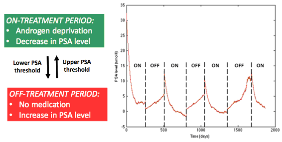
Figure 1: Schematic representation of Intermittent Androgen Suppression (IAS) therapy

An event set $E=\left\{e_{1},e_{2}\right\}$, where $e_{1}$ corresponds to the condition $\left[x_{1}\left(t\right)+x_{2}\left(t\right)=\theta_{1}\text{ from above}\right]$ (i.e., $x_{1}\left(t^{-}\right)+x_{2}\left(t^{-}\right)>\theta_{1}$) and $e_{2}$ corresponds to the condition $\left[x_{1}\left(t\right)+x_{2}\left(t\right)=\theta_{2}\text{ from below}\right]$ (i.e., $x_{1}\left(t^{-}\right)+x_{2}\left(t^{-}\right)<\theta_{2}$), where the notation $t^{-}$ indicates the time instant immediately preceding time $t$.

System dynamics describing the evolution of continuous state variables over time, as well as the rules for discrete state transitions. The continuous (time-driven) dynamics capture the prostate cancer cell population dynamics, which are defined in terms of their proliferation, apoptosis, and conversion rates. As in [5], we incorporate stochastic effects into the deterministic model from [11] as follows:

$$\begin{array}[c]{ll}\dot{x}_{1}(t)&=\alpha_{1}\left[1+e^{-\left(x_{3}(t)-k_{1}\right)k_{2}}\right]^{-1}\cdot x_{1}(t)\\ &-\beta_{1}\left[1+e^{-\left(x_{3}(t)-k_{3}\right)k_{4}}\right]^{-1}\cdot x_{1}(t)\\ &-\left[m_{1}\left(1-\frac{x_{3}(t)}{x_{3,0}}\right)+\lambda_{1}\right]\cdot x_{1}(t)\\ &+\mu_{1}+\zeta_{1}(t)\end{array}$$ (2)

$$\begin{array}[]{ll}\dot{x}_{2}(t)=&\left[\alpha_{2}\left(1-d\frac{x_{3}(t)}{x_{3,0}}\right)-\beta_{2}\right]x_{2}(t)\\ &+m_{1}\left(1-\frac{x_{3}(t)}{x_{3,0}}\right)x_{1}(t)+\zeta_{2}(t)\end{array}$$ (3)

$$\dot{x}_{3}(t)=\left\{\begin{array}[]{ll}-\frac{x_{3}(t)}{\sigma}+\mu_{3}+\zeta_{3}(t)&\begin{array}[]{l}\text{if }x_{1}(t)+x_{2}(t)>\theta_{1}\\ \text{and }q(t)=q^{ON}\end{array}\text{ }\\ \frac{x_{3,0}-x_{3}(t)}{\sigma}+\mu_{3}+\zeta_{3}(t)&\begin{array}[]{l}\text{if }x_{1}(t)+x_{2}(t)<\theta_{2}\text{ }\\ \text{and }q(t)=q^{OFF}\end{array}\end{array}\right.$$ (4)

$$\dot{z}_{1}(t) =\left\{\begin{array}[]{ll}1&\text{if }q(t)=q^{ON}\\ 0&\text{otherwise}\end{array}\right.$$ (7)

$$z_{1}(t^{+}) =\begin{array}[t]{ll}0&\begin{array}[]{l}\text{if }x_{1}(t)+x_{2}(t)=\theta_{1}\\ \text{and }q(t)=q^{ON}\end{array}\text{ }\end{array}$$ (11)

$$\dot{z}_{2}(t) =\left\{\begin{array}[]{ll}1&\text{if }q(t)=q^{OFF}\\ 0&\text{otherwise}\end{array}\right.$$ (14)

$$z_{2}(t^{+}) =\begin{array}[t]{ll}0&\begin{array}[]{l}\text{if }x_{1}(t)+x_{2}(t)=\theta_{2}\\ \text{and }q(t)=q^{OFF}\text{ }\end{array}\end{array}$$ (18)

where $\alpha_{1}$ and $\alpha_{2}$ are the HSC proliferation constant and CRC proliferation constant, respectively; $\beta_{1}$ and $\beta_{2}$ are the HSC apoptosis constant and CRC apoptosis constant, respectively; $k_{1}$ through $k_{4}$ are HSC proliferation and apoptosis exponential constants; $m_{1}$ is the HSC to CRC conversion constant; $x_{3,0}$ corresponds to the patient-specific androgen constant; $\sigma$ is the androgen degradation constant; $\lambda_{1}$ is the HSC basal degradation rate; $\mu_{1}$ and $\mu_{3}$ are the HSC basal production rate and androgen basal production rate, respectively. Finally, $\{\zeta_{i}(t)\}$, $i=1,2,3$, are stochastic processes which we allow to have arbitrary characteristics and only assume them to be piecewise continuous w.p. 1. The processes $\{\zeta_{i}(t)\}$, $i=1,2$, represent noise and fluctuations inherently associated with cell population dynamics, while $\{\zeta_{3}(t)\}$ reflects randomness associated with monitoring clinical data, more specifically, with monitoring the patient’s androgen level.

It is clear from (2)-(4) that $x_{1}\left(t\right)$ and $x_{2}\left(t\right)$ are dependent on $x_{3}\left(t\right)$, whose dynamics are affected by mode transitions. To make explicit the dependence of $x_{1}\left(t\right)$ and $x_{2}\left(t\right)$ on the discrete state (mode) $q\left(t\right)$, we let $\tau_{k}\left(\tilde{\theta}\right)$ be the time of occurrence of the $k$th event (of any type), and denote the state dynamics over any interevent interval $\left[\tau_{k}\left(\tilde{\theta}\right),\tau_{k+1}\left(\tilde{\theta}\right)\right)$ as

$$\dot{x}_{n}(t)=f_{k}^{x_{n}}(t)\text{, }\dot{z}_{i}(t)=f_{k}^{z_{i}}(t)\text{ , }n=1,\ldots,3\text{, }i=1,2$$

We include $\tilde{\theta}$ as an argument to stress the dependence of the event times on the controllable parameters, but we will subsequently drop this for ease of notation as long as no confusion arises.

We thus start by assuming $q(t)=q^{ON}$ for $t\in$ $\left[\tau_{k},\tau_{k+1}\right)$. Solving (4) yields, for $t\in$ $\left[\tau_{k},\tau_{k+1}\right)$,

$$\begin{array}[]{ll}x_{3}(t)&=x_{3}(\tau_{k}^{+})e^{-\left(t-\tau_{k}\right)/\sigma}\\ &+e^{-t/\sigma}\cdot\int_{\tau_{k}}^{t}e^{\varepsilon/\sigma}\left[\mu_{3}+\zeta_{3}(\varepsilon)\right]d\varepsilon\end{array}$$

It is then possible to define, for $t\in$ $\left[\tau_{k},\tau_{k+1}\right)$,

$$\begin{array}[]{ll}h^{ON}\left(t,\tilde{\zeta}_{3}(t)\right)&\equiv x_{3}(\tau_{k}^{+})e^{-\left(t-\tau_{k}\right)/\sigma}\\ &+\mu_{3}\sigma[1-e^{-\left(t-\tau_{k}\right)/\sigma}]+\tilde{\zeta}_{3}(t)\end{array}$$ (19)

where, for notational simplicity, we let

$$\tilde{\zeta}_{3}(t)=\int_{\tau_{k}}^{t}e^{-\left(t-\varepsilon\right)/\sigma}\zeta_{3}(\varepsilon)d\varepsilon$$ (20)

Next, let $q(t)=q^{OFF}$ for $t\in$ $\left[\tau_{k},\tau_{k+1}\right)$, so that (4) implies that, for $t\in$ $\left[\tau_{k},\tau_{k+1}\right)$,

$$\begin{array}[]{ll}x_{3}(t)&=x_{3}(\tau_{k}^{+})e^{-\left(t-\tau_{k}\right)/\sigma}\\ &+(\mu_{3}\sigma+x_{3,0})[1-e^{-\left(t-\tau_{k}\right)/\sigma}]+\tilde{\zeta}_{3}(t)\end{array}$$

Similarly as above, we define, for $t\in$ $\left[\tau_{k},\tau_{k+1}\right)$,

$$\begin{array}[]{ll}h^{OFF}\left(t,\tilde{\zeta}_{3}(t)\right)&\equiv x_{3}(\tau_{k}^{+})e^{-\left(t-\tau_{k}\right)/\sigma}\\ &+(\mu_{3}\sigma+x_{3,0})[1-e^{-\left(t-\tau_{k}\right)/\sigma}]+\tilde{\zeta}_{3}(t)\end{array}$$ (21)

It is then possible to rewrite (4) as follows:

$$x_{3}(t)=\left\{\begin{array}[]{ll}h^{ON}\left(t,\tilde{\zeta}_{3}(t)\right)&\text{if }q(t)=q^{ON}\\ h^{OFF}\left(t,\tilde{\zeta}_{3}(t)\right)&\text{if }q(t)=q^{OFF}\end{array}\right.$$

Although we include $\tilde{\zeta}_{3}(t)$ as an argument in (19 ) and (21) to stress the dependence on the stochastic process, we will subsequently drop this for ease of notation as long as no confusion arises. Hence, substituting (19) and (21) into (2)-(3), yields

$$\dot{x}_{1}(t)=\left\{\begin{array}[]{l}\begin{array}[]{l}\left\{\alpha_{1}\left[1+\phi_{\alpha}^{ON}(t)\right]^{-1}-\beta_{1}\left[1+\phi_{\beta}^{ON}(t)\right]^{-1}\right.\\ \left.+m_{1}\left(\frac{h^{ON}\left(t\right)}{x_{3,0}}\right)-(m_{1}+\lambda_{1})\right\}\cdot x_{1}(t)\\ +\mu_{1}+\zeta_{1}(t)\text{ \ \ \ \ \ \ \ \ \ \ \ \ \ \ \ \ \ \ \ \ \ \ \ \ if }q(t)=q^{ON}\end{array}\\ \begin{array}[]{l}\left\{\alpha_{1}\left[1+\phi_{\alpha}^{OFF}(t)\right]^{-1}-\beta_{1}\left[1+\phi_{\beta}^{OFF}(t)\right]^{-1}\right.\\ \left.+m_{1}\left(\frac{h^{OFF}\left(t\right)}{x_{3,0}}\right)-(m_{1}+\lambda_{1})\right\}\cdot x_{1}(t)\\ +\mu_{1}+\zeta_{1}(t)\text{ \ \ \ \ \ \ \ \ \ \ \ \ \ \ \ \ \ \ \ \ \ \ \ \ if }q(t)=q^{OFF}\end{array}\end{array}\right.$$ (22)

$$\dot{x}_{2}(t)=\left\{\begin{array}[]{l}\begin{array}[]{l}\left[\alpha_{2}\left(1-d\frac{h^{ON}\left(t\right)}{x_{3,0}}\right)-\beta_{2}\right]x_{2}(t)\\ +m_{1}\left(1-\frac{h^{ON}\left(t\right)}{x_{3,0}}\right)x_{1}(t)+\zeta_{2}(t)\\ \text{ \ \ \ \ \ \ \ \ \ \ \ \ \ \ \ \ \ \ \ \ \ \ \ \ \ \ \ \ if }q(t)=q^{ON}\end{array}\\ \begin{array}[]{l}\left[\alpha_{2}\left(1-d\frac{h^{OFF}\left(t\right)}{x_{3,0}}\right)-\beta_{2}\right]x_{2}(t)\\ +m_{1}\left(1-\frac{h^{OFF}\left(t\right)}{x_{3,0}}\right)x_{1}(t)+\zeta_{2}(t)\\ \text{ \ \ \ \ \ \ \ \ \ \ \ \ \ \ \ \ \ \ \ \ \ \ \ \ \ \ \ if }q(t)=q^{OFF}\end{array}\end{array}\right.$$ (23)

with

$$\phi_{\alpha}^{ON}(t) =e^{-\left(h^{ON}\left(t\right)-k_{1}\right)k_{2}}$$

$$\phi_{\beta}^{ON}(t) =e^{-\left(h^{ON}\left(t\right)-k_{3}\right)k_{4}}$$

$$\phi_{\alpha}^{OFF}(t) =e^{-\left(h^{OFF}\left(t\right)-k_{1}\right)k_{2}}$$

$$\phi_{\beta}^{OFF}(t) =e^{-\left(h^{OFF}\left(t\right)-k_{3}\right)k_{4}}$$

The discrete (event-driven) dynamics are dictated by the occurrence of events that cause state transitions. Based on the event set $E=\left\{e_{1},e_{2}\right\}$ we have defined, the occurrence of $e_{1}$ results in a transition from $q^{ON}$ to $q^{OFF}$ and the occurrence of $e_{2}$ results in a transition from $q^{OFF}$ to $q^{ON}$.

II-B IAS Sensitivity Analysis

Recall that the main goal of this work is to perform sensitivity analysis of (2)-(14) in order to identify critical model parameters and verify the extent to which the SHA model of prostate cancer evolution is robust to them. Of note, several potentially critical parameters exist in the SHA model from [5]. This work is a first step towards analyzing their relative importance, in which we select a subset of all model parameters in order to illustrate the applicability of our IPA-based methodology. The parameters we consider here are $\alpha_{1}$ and $\alpha_{2}$ (HSC proliferation constant and CRC proliferation constant, respectively), as well as $\beta_{1}$ and $\beta_{2}$ (HSC apoptosis constant and CRC apoptosis constant, respectively). These constants are intrinsically related to the cancer cell subpopulations’ net growth rate, whose value dictates how fast the PSA threshold values will be reached, and ultimately how soon treatment will be suspended or reinstated. As a result, correctly estimating the values of $\alpha_{i}$ and $\beta_{i}$, $i=1,2$, is presumably crucial for the purposes of personalized IAS therapy design.

In this context, we define an extended parameter vector $\mathbf{\tilde{\theta}}=\left[\tilde{\theta}_{1},\ldots,\tilde{\theta}_{6}\right]$, where $\tilde{\theta}_{1}$ ($\tilde{\theta}_{2}$, respectively) corresponds to the lower (upper, respectively) threshold value of the patient’s PSA level, $\tilde{\theta}_{3}$ ($\tilde{\theta}_{4}$, respectively) corresponds to the HSC (CRC, respectively) proliferation constant, and $\tilde{\theta}_{5}$ ($\tilde{\theta}_{6}$, respectively) corresponds to the HSC (CRC, respectively) apoptosis constant.

Within the SHA framework presented above, an IAS therapy can be viewed as a controlled process $u\left(\tilde{\theta},t\right)$ characterized by the parameter vector $\tilde{\theta}$, as in (1), whose effect can be quantified in terms of performance metrics of the form $J\left[u\left(\tilde{\theta},t\right)\right]$. Of note, only the first two elements in vector $\tilde{\theta}$ are controllable, while the remaining parameters are not.

As in [5], here we make use of a sample function defined in terms of complementary measures of therapy success. In particular, we consider the most adequate IAS treatment schemes to be those that $(i)$ ensure PSA levels are kept as low as possible; $(ii)$ reduce the frequency of on and off-treatment cycles. From a practical perspective, $(i)$ translates into the ability to successfully keep the size of cancer cell populations under control, which is directly influenced by the duration of the on and off-treatment periods. On the other hand, $(ii)$ aims at reducing the duration of on-treatment periods, thus decreasing the exposure of patients to medication and their side effects, and consequently improving the patients’ quality of life throughout the treatment. Clearly there is a trade-off between keeping tumor growth under control and the cost associated with the corresponding IAS therapy. The latter is related to the duration of the therapy and could potentially include fixed set up costs incurred when therapy is reinstated. For simplicity, we disconsider fixed set up costs and take $(ii)$ to be linearly proportional to the length of the on-treatment cycles. Hence, we define our sample function as the sum of the average PSA level and the average duration of an on-treatment cycle over a fixed time interval $\left[0,T\right]$. We also take into account that it may be desirable to design a therapy scheme which favors $(i)$ over $(ii)$ (or vice-versa) and thus associate weight $W$ with $(i)$ and $1-W$ with $(ii)$, where $0\leq W\leq 1$. Finally, to ensure that the trade-off between $(i)$ and $(ii)$ is captured appropriately, we normalize our sample function: we divide $(i)$ by the value of the patient’s PSA level at the start of the first on-treatment cycle ($PSA_{init}$), and normalize $(ii)$ by $T$.

Recall that the total population size of prostate cancer cells is assumed to reflect the serum PSA concentration, and that we have defined clock variables which measure the time elapsed in each of the treatment modes, so that our sample function can be written as

$$L\left(\theta,x(0),z(0),T\right)=\begin{array}[t]{l}\frac{W}{T}\overset{T}{\underset{0}{\int}}\left[\frac{x_{1}\left(\theta,t\right)+x_{2}\left(\theta,t\right)}{PSA_{init}}\right]dt\\ +\frac{(1-W)}{T}\overset{T}{\underset{0}{\int}}\frac{z_{1}\left(t\right)}{T}dt\end{array}$$ (24)

where $x(0)$ and $z(0)$ are given initial conditions. We can then define the overall performance metric as

$$J\left(\tilde{\theta},x(0),z(0),T\right)=E\left[L\left(\tilde{\theta},x(0),z(0),T\right)\right]$$ (25)

We note that it is not possible to derive a closed-form expression of $J\left(\tilde{\theta},x(0),z(0),T\right)$ without imposing limitations on the processes $\{\zeta_{i}(t)\}$, $i=1,\ldots,3$. Nevertheless, by assuming only that $\zeta_{i}(t)$, $i=1,\ldots,3$, are piecewise continuous w.p. 1, we can successfully apply the IPA methodology developed for general SHS in [4] and obtain an estimate of $\nabla J\left(\tilde{\theta}\right)$ by evaluating the sample gradient $\nabla L\left(\tilde{\theta}\right)$. We will assume that the derivatives $dL\left(\tilde{\theta}\right)/d\tilde{\theta}_{i}$ exist w.p. 1 for all $\tilde{\theta}_{i}\in\mathbb{R}^{+}$. It is also simple to verify that $L\left(\tilde{\theta}\right)$ is Lipschitz continuous for $\tilde{\theta}_{i}$ in $\mathbb{R}^{+}$. We will further assume that $\{\zeta_{i}(t)\}$, $i=1,\ldots,3$, are stationary random processes over $\left[0,T\right]$ and that no two events can occur at the same time w.p. 1. Under these conditions, it has been shown in [4] that $dL\left(\tilde{\theta}\right)/d\tilde{\theta}_{i}$ is an unbiased estimator of $dJ\left(\tilde{\theta}\right)/d\tilde{\theta}_{i}$, $i=1,\ldots,6$. Hence, our goal is to compute the sample gradient $\nabla L\left(\tilde{\theta}\right)$ using data extracted from a sample path of the system (e.g., by simulating a sample path of our SHA model using clinical data), and use this value as an estimate of $\nabla J\left(\tilde{\theta}\right)$.

III Infinitesimal Perturbation Analysis

For completeness, we provide here a brief overview of the IPA framework developed for stochastic hybrid systems in [4]. For such, we adopt a standard SHA definition [3]:

$$G_{h}=\left(Q,X,E,U,f,\phi,Inv,guard,\rho,q_{0},x_{0}\right)$$ (26)

where $Q$ is a set of discrete states; $X$ is a continuous state space; $E$ is a finite set of events; $U$ is a set of admissible controls; $f$ is a vector field, $f:Q\times X\times U\rightarrow X$; $\phi$ is a discrete state transition function, $\phi:Q\times X\times E\rightarrow Q$; $Inv$ is a set defining an invariant condition (when this condition is violated at some $q\in Q$, a transition must occur); $guard$ is a set defining a guard condition, $guard\subseteq Q\times Q\times X$ (when this condition is satisfied at some $q\in Q$, a transition is allowed to occur); $\rho$ is a reset function, $\rho:Q\times Q\times X\times E\rightarrow X$; $q_{0}$ is an initial discrete state; $x_{0}$ is an initial continuous state.

Consider a sample path of the system over $\left[0,T\right]$ and denote the time of occurrence of the $k$th event (of any type) by $\tau_{k}\left(\theta\right)$, where $\theta$ corresponds to the control parameter of interest. Although we use the notation $\tau_{k}\left(\theta\right)$ to stress the dependency of the event time on the control parameter, we will subsequently use $\tau_{k}$ to indicate the time of occurrence of the $k$th event where no confusion arises. In order to further simplify notation, we shall denote the state and event time derivatives with respect to parameter $\theta$ as $x^{\prime}(t)\equiv\frac{\partial x(\theta,t)}{\partial\theta}$ and $\tau_{k}^{\prime}\equiv\frac{\partial\tau_{k}}{\partial\theta}$, respectively, for $k=1,...,N$. Additionally, considering that the system is at some discrete mode during an interval $\left[\tau_{k},\tau_{k+1}\right)$, we will denote its time-driven dynamics over such interval as $f_{k}\left(x,\theta,t\right)$. It is shown in [4] that the state derivative satisfies

$$\frac{d}{dt}x^{\prime}(t)=\frac{\partial f_{k}(t)}{\partial x}x^{\prime}(t)+\frac{\partial f_{k}(t)}{\partial\theta}$$ (27)

with the following boundary condition:

$$x^{\prime}(\tau_{k}^{+})=x^{\prime}(\tau_{k}^{-})+\left[f_{k-1}(\tau_{k}^{-})-f_{k}(\tau_{k}^{+})\right].\tau_{k}^{\prime}$$ (28)

when $x(\theta,t)$ is continuous in $t$ at $t=\tau_{k}$. Otherwise,

$$x^{\prime}(\tau_{k}^{+})=\frac{d\rho\left(q,q^{\prime},x,e\right)}{d\theta}$$ (29)

where $\rho\left(q,q^{\prime},x,e\right)$ is the reset function defined in (26).

Knowledge of $\tau_{k}^{\prime}$ is, therefore, needed in order to evaluate (28). Following the framework in [4], there are three types of events for a general stochastic hybrid system: (i) Exogenous event. This type of event causes a discrete state transition which is independent of parameter $\theta$ and, as a result, $\tau_{k}^{\prime}=0$. (ii) Endogenous event. In this case, there exists a continuously differentiable function $g_{k}:\Re^{n}\times\Theta\rightarrow\Re$ such that $\tau_{k}=\min\left\{t>\tau_{k-1}:g_{k}\left(x(\theta,t),\theta\right)=0\right\}$, which leads to

$$\tau_{k}^{\prime}=-\left[\frac{\partial g_{k}}{\partial x}.f_{k-1}(\tau_{k}^{-})\right]^{-1}.\left(\frac{\partial g_{k}}{\partial\phi}+\frac{\partial g_{k}}{\partial x}.x^{\prime}(\tau_{k}^{-})\right)$$ (30)

where $\frac{\partial g_{k}}{\partial x}.f_{k-1}(\tau_{k}^{-})\neq 0$. (iii) Induced event. Such an event is triggered by the occurrence of another event at time $\tau_{m}\leq\tau_{k}$ and the expression of $\tau_{k}^{\prime}$ depends on the event time derivative of the triggering event ($\tau_{m}^{\prime}$) (details can be found in [4]).

Thus, IPA captures how changes in $\theta$ affect the event times and the state of the system. Since interesting performance metrics are usually expressed in terms of $\tau_{k}$ and $x(t)$, IPA can ultimately be used to infer the effect that a perturbation in $\theta$ will have on such metrics. We end this overview by returning to our problem of personalized prostate cancer therapy design and thus defining the derivatives of the states $x_{n}(\tilde{\theta},t)$ and $z_{j}(\tilde{\theta},t)$ and event times $\tau_{k}(\tilde{\theta})$ with respect to $\tilde{\theta}_{i}$, $i=1,\ldots,6$, $j=1,2$, $n=1,\ldots,3$, as follows:

$$x_{n,i}^{\prime}(t)\equiv\frac{\partial x_{n}(\tilde{\theta},t)}{\partial\tilde{\theta}_{i}}\text{, \ }z_{j,i}^{\prime}(t)\equiv\frac{\partial z_{j}(\tilde{\theta},t)}{\partial\tilde{\theta}_{i}},\text{ }\tau_{k,i}^{\prime}\equiv\frac{\partial\tau_{k}(\tilde{\theta})}{\partial\tilde{\theta}_{i}}$$ (31)

In what follows, we derive the IPA state and event time derivatives for the events identified in the SHA model of prostate cancer progression.

III-A State and Event Time Derivatives

We proceed by analyzing the state evolution of our SHA model of prostate cancer progression considering each of the states ($q^{ON}$ and $q^{OFF}$) and events ($e_{1}$ and $e_{2}$) therein defined.

1. The system is in state $q^{ON}$ over interevent time interval $\left[\tau_{k},\tau_{k+1}\right)$. Using (27) for $x_{1}\left(t\right)$, we obtain, for $i=1,\ldots,6$,

$$\begin{array}[]{ll}\frac{d}{dt}x_{1,i}^{\prime}(t)&=\frac{\partial f_{k}^{x_{1}}(t)}{\partial x_{1}}x_{1}^{\prime}(t)+\frac{\partial f_{k}^{x_{1}}(t)}{\partial x_{2}}x_{2}^{\prime}(t)\\ &+\frac{\partial f_{k}^{x_{1}}(t)}{\partial z_{1}}z_{1}^{\prime}(t)+\frac{\partial f_{k}^{x_{1}}(t)}{\partial z_{2}}z_{2}^{\prime}(t)+\frac{\partial f_{k}^{x_{1}}(t)}{\partial\tilde{\theta}_{i}}\end{array}$$

From (22), we have $\frac{\partial f_{k}^{x_{1}}(t)}{\partial x_{2}}=\frac{\partial f_{k}^{x_{1}}(t)}{\partial z_{j}}=\frac{\partial f_{k}^{x_{1}}(t)}{\partial\tilde{\theta}_{i}}=0$, $i=1,2,4,6$, $j=1,2$, and

$$\begin{array}[]{ll}\frac{\partial f_{k}^{x_{1}}(t)}{\partial x_{1}}&=\alpha_{1}\left[1+\phi_{\alpha}^{ON}(t)\right]^{-1}-\beta_{1}\left[1+\phi_{\beta}^{ON}(t)\right]^{-1}\\ &-m_{1}\left(1-\frac{h^{ON}\left(t\right)}{x_{3,0}}\right)-\lambda_{1}\end{array}$$

$$\begin{array}[]{ll}\frac{\partial f_{k}^{x_{1}}(t)}{\partial\tilde{\theta}_{3}}&=x_{1}\left[1+\phi_{\alpha}^{ON}(t)\right]^{-1}\end{array}$$

$$\begin{array}[]{ll}\frac{\partial f_{k}^{x_{1}}(t)}{\partial\tilde{\theta}_{5}}&=-x_{1}\left[1+\phi_{\beta}^{ON}(t)\right]^{-1}\end{array}$$

It is thus simple to verify that solving (27) for $x_{1,i}^{\prime}(t)$ yields, for $t\in\left[\tau_{k},\tau_{k+1}\right)$,

$$x_{1,i}^{\prime}(t)=x_{1,i}^{\prime}(\tau_{k}^{+})e^{A_{1}\left(t\right)}\text{, \ }i=1,2,4,6$$ (35)

$$x_{1,3}^{\prime}(t)=x_{1,3}^{\prime}(\tau_{k}^{+})e^{A_{1}\left(t\right)}+A_{2}\left(t\right)$$ (36)

$$x_{1,5}^{\prime}(t)=x_{1,5}^{\prime}(\tau_{k}^{+})e^{A_{1}\left(t\right)}+A_{3}\left(t\right)$$ (37)

with

$$\begin{array}[]{l}A_{1}\left(t\right)\equiv\int_{\tau_{k}}^{t}\left[\frac{\alpha_{1}}{1+\phi_{\alpha}^{ON}(t)}-\frac{\beta_{1}}{1+\phi_{\beta}^{ON}(t)}\right]dt\\ \text{ \ }-\int_{\tau_{k}}^{t}\frac{m_{1}}{x_{3,0}}h^{ON}\left(t\right)dt-\left(m_{1}+\lambda_{1}\right)\left(t-\tau_{k}\right)\end{array}$$ (40)

$$A_{2}\left(t\right)\equiv e^{A_{1}\left(t\right)}\int_{\tau_{k}}^{t}\left[\frac{x_{1}\left(t\right)}{1+\phi_{\alpha}^{ON}(t)}e^{-A_{1}\left(t\right)}\right]dt$$ (41)

$$A_{3}\left(t\right)\equiv e^{A_{1}\left(t\right)}\int_{\tau_{k}}^{t}\left[-\frac{x_{1}\left(t\right)}{1+\phi_{\beta}^{ON}(t)}e^{A_{1}\left(t\right)}\right]dt$$ (42)

In particular, at $\tau_{k+1}^{-}$:

$$x_{1,i}^{\prime}(\tau_{k+1}^{-})=x_{1,i}^{\prime}(\tau_{k}^{+})e^{A\left(\tau_{k}\right)}$$ (43)

$$x_{1,3}^{\prime}(\tau_{k+1}^{-})=x_{1,3}^{\prime}(\tau_{k}^{+})e^{A\left(\tau_{k}\right)}+A_{2}\left(\tau_{k}\right)$$ (44)

$$x_{1,5}^{\prime}(\tau_{k+1}^{-})=x_{1,5}^{\prime}(\tau_{k}^{+})e^{A\left(\tau_{k}\right)}+A_{3}\left(\tau_{k}\right)$$ (45)

where $A_{1}\left(\tau_{k}\right)$, $A_{2}\left(\tau_{k}\right)$, and $A_{3}\left(\tau_{k}\right)$ are given from (40).

Similarly for $x_{2}\left(t\right)$, we have from (23) that $\frac{\partial f_{k}^{x_{2}}(t)}{\partial z_{j}}=\frac{\partial f_{k}^{x_{2}}(t)}{\partial\tilde{\theta}_{i}}=0$, $i=1,2,3,5$, $j=1,2$, and

$$\begin{array}[]{l}\frac{\partial f_{k}^{x_{2}}(t)}{\partial x_{1}}=m_{1}\left(1-\frac{h^{ON}\left(t\right)}{x_{3,0}}\right)\\ \frac{\partial f_{k}^{x_{2}}(t)}{\partial x_{2}}=\alpha_{2}\left(1-d\frac{h^{ON}\left(t\right)}{x_{3,0}}\right)-\beta_{2}\\ \frac{\partial f_{k}^{x_{2}}(t)}{\partial\tilde{\theta}_{4}}=\left(1-d\frac{h^{ON}\left(t\right)}{x_{3,0}}\right)x_{2}\left(t\right)\\ \frac{\partial f_{k}^{x_{2}}(t)}{\partial\tilde{\theta}_{6}}=-x_{2}\left(t\right)\end{array}$$

Combining the last four equations and solving for $x_{2,i}^{\prime}(t)$ yields, for $t\in\left[\tau_{k},\tau_{k+1}\right)$,

$$x_{2,i}^{\prime}(t)=x_{2,i}^{\prime}(\tau_{k}^{+})e^{B_{1}(t)}+B_{2}\left(t,x_{1,i}^{\prime}(\tau_{k}^{+}),A_{1}\left(t\right)\right)\text{, \ \ }i=1,2,3,5$$ (46)

$$x_{2,4}^{\prime}(t)=x_{2,4}^{\prime}(\tau_{k}^{+})e^{B_{1}(t)}+B_{3}\left(t,x_{1,4}^{\prime}(\tau_{k}^{+}),B_{1}\left(t\right)\right)$$ (47)

$$x_{2,6}^{\prime}(t)=x_{2,6}^{\prime}(\tau_{k}^{+})e^{B_{1}(t)}+B_{4}\left(t,x_{1,6}^{\prime}(\tau_{k}^{+}),B_{1}\left(t\right)\right)$$ (48)

with

$$B_{1}\left(t\right)\equiv\int_{\tau_{k}}^{t}\left[\alpha_{2}\left(1-d\frac{h^{ON}\left(t\right)}{x_{3,0}}\right)-\beta_{2}\right]dt$$ (49)

$$B_{2}\left(\cdot\right)\equiv e^{B_{1}(t)}\int_{\tau_{k}}^{t}G_{1}\left(t,\tau_{k}\right)e^{-B_{1}(t)}dt$$

$$B_{3}\left(\cdot\right)\equiv e^{B_{1}(t)}\int_{\tau_{k}}^{t}G_{2}\left(t,\tau_{k}\right)e^{-B_{1}(t)}dt$$ (50)

$$B_{4}\left(\cdot\right)\equiv e^{B_{1}(t)}\int_{\tau_{k}}^{t}G_{3}\left(t,\tau_{k}\right)e^{-B_{1}(t)}dt$$ (51)

where $G_{1}\left(t,\tau_{k}\right)=m_{1}\left(1-\frac{h^{ON}\left(t\right)}{x_{3,0}}\right)x_{1,i}^{\prime}(\tau_{k}^{+})e^{A_{1}\left(t\right)}$, $G_{2}\left(t,\tau_{k}\right)=e^{-B_{1}(t)}x_{2}\left(t\right)\left(1-d\frac{h^{ON}\left(t\right)}{x_{3,0}}\right)$$+e^{-B_{1}(t)}x_{1,4}^{\prime}(t)\cdot m_{1}\left(1-d\frac{h^{ON}\left(t\right)}{x_{3,0}}\right)$, $G_{3}\left(t,\tau_{k}\right)=e^{-B_{1}(t)}\left[x_{1,6}^{\prime}(t)\cdot m_{1}\left(1-d\frac{h^{ON}\left(t\right)}{x_{3,0}}\right)-x_{2}\left(t\right)\right]$, $t\in\left[\tau_{k},\tau_{k+1}\right)$.

In particular, at $\tau_{k+1}^{-}$:

$$x_{2,i}^{\prime}(\tau_{k+1}^{-})=x_{2,i}^{\prime}(\tau_{k}^{+})e^{B_{1}(\tau_{k})}+B_{2}\left(\tau_{k},x_{1,i}^{\prime}(\tau_{k}^{+}),A\left(\tau_{k}\right)\right)$$ (52)

$$x_{2,4}^{\prime}(\tau_{k+1}^{-})=x_{2,4}^{\prime}(\tau_{k}^{+})e^{B_{1}(\tau_{k})}+B_{3}\left(t,x_{1,4}^{\prime}(\tau_{k}^{+}),B_{1}\left(\tau_{k}\right)\right)$$ (53)

$$x_{2,6}^{\prime}(\tau_{k+1}^{-})=x_{2,6}^{\prime}(\tau_{k}^{+})e^{B_{1}(\tau_{k})}+B_{4}\left(t,x_{1,6}^{\prime}(\tau_{k}^{+}),B_{1}\left(\tau_{k}\right)\right)$$ (54)

where $B_{1}\left(\tau_{k}\right)$, $B_{2}\left(\tau_{k},x_{1,i}^{\prime}(\tau_{k}^{+}),A\left(\tau_{k}\right)\right)$, $B_{3}\left(t,x_{1,4}^{\prime}(\tau_{k}^{+}),B_{1}\left(\tau_{k}\right)\right)$, and $B_{4}\left(t,x_{1,6}^{\prime}(\tau_{k}^{+}),B_{1}\left(\tau_{k}\right)\right)$ are given from (49).

Finally, for the “clock” state variable, from (7)-(14) we have $\frac{\partial f_{k}^{z_{i}}(t)}{\partial x_{n}}=\frac{\partial f_{k}^{z_{i}}(t)}{\partial z_{j}}=\frac{\partial f_{k}^{z_{i}}(t)}{\partial\tilde{\theta}_{i}}=0$, $n,j=1,2$, $i=1,\ldots,6$, so that $\frac{d}{dt}z_{j,i}^{\prime}(t)=0$, $j=1,2$, $i=1,\ldots,6$, for $t\in\left[\tau_{k},\tau_{k+1}\right)$. Hence, $z_{j,i}^{\prime}(t)=z_{j,i}^{\prime}(\tau_{k}^{+})$, $j=1,2$, $i=1,\ldots,6$, and $t\in\left[\tau_{k},\tau_{k+1}\right)$.

2. The system is in state $q^{OFF}$ over interevent time interval $\left[\tau_{k},\tau_{k+1}\right)$. Starting with $x_{1}\left(t\right)$, based on (22) we once again have $\frac{\partial f_{k}^{x_{1}}(t)}{\partial x_{2}}=\frac{\partial f_{k}^{x_{1}}(t)}{\partial zj}=\frac{\partial f_{k}^{x_{1}}(t)}{\partial\tilde{\theta}_{i}}=0$, $j=1,2$, $i=1,2,4,6$, but now

$$\begin{array}[]{l}\frac{\partial f_{k}^{x_{1}}(t)}{\partial x_{1}}=\alpha_{1}\left[1+\phi_{\alpha}^{OFF}(t)\right]^{-1}-\beta_{1}\left[1+\phi_{\beta}^{OFF}(t)\right]^{-1}\\ \text{ \ \ \ \ \ \ \ \ }-m_{1}\left(1-\frac{h^{OFF}\left(t\right)}{x_{3,0}}\right)-\lambda_{1}\end{array}$$

$$\begin{array}[]{ll}\frac{\partial f_{k}^{x_{1}}(t)}{\partial\tilde{\theta}_{3}}&=x_{1}\left[1+\phi_{\alpha}^{ON}(t)\right]^{-1}\end{array}$$

$$\begin{array}[]{ll}\frac{\partial f_{k}^{x_{1}}(t)}{\partial\tilde{\theta}_{5}}&=-x_{1}\left[1+\phi_{\beta}^{ON}(t)\right]^{-1}\end{array}$$

Therefore, (27) implies that, for $t\in\left[\tau_{k},\tau_{k+1}\right)$:

$$x_{1,i}^{\prime}(t)=x_{1,i}^{\prime}(\tau_{k}^{+})e^{C_{1}\left(t\right)}\text{, \ }i=1,2,4,6$$ (58)

$$x_{1,3}^{\prime}(t)=x_{1,3}^{\prime}(\tau_{k}^{+})e^{C_{1}\left(t\right)}+C_{2}\left(t\right)$$ (59)

$$x_{1,5}^{\prime}(\tau_{k+1}^{-})=x_{1,5}^{\prime}(\tau_{k}^{+})e^{C_{1}\left(\tau_{k}\right)}+C_{3}\left(t\right)$$ (60)

with

$$\begin{array}[]{l}C_{1}\left(t\right)\equiv\int_{\tau_{k}}^{t}\left[\frac{\alpha_{1}}{1+\phi_{\alpha}^{OFF}(t)}-\frac{\beta_{1}}{1+\phi_{\beta}^{OFF}(t)}\right]dt\\ \text{ }-\int_{\tau_{k}}^{t}\frac{m_{1}}{x_{3,0}}h^{OFF}\left(t\right)dt-\left(m_{1}+\lambda_{1}\right)\left(t-\tau_{k}\right)\end{array}$$ (63)

$$C_{2}\left(t\right)\equiv e^{C_{1}\left(t\right)}\int_{\tau_{k}}^{t}\left[\frac{x_{1}\left(t\right)}{1+\phi_{\alpha}^{OFF}(t)}e^{-C_{1}\left(t\right)}\right]dt$$ (64)

$$C_{3}\left(t\right)\equiv e^{C_{1}\left(\tau_{k}\right)}\int_{\tau_{k}}^{\tau_{k+1}}\left[-\frac{x_{1}\left(t\right)}{1+\phi_{\beta}^{OFF}(t)}e^{C_{1}\left(t\right)}\right]dt$$ (65)

In particular, at $\tau_{k+1}^{-}$:

$$x_{1,i}^{\prime}(\tau_{k+1}^{-})=x_{1,i}^{\prime}(\tau_{k}^{+})e^{C_{1}\left(\tau_{k}\right)}$$ (66)

$$x_{1,3}^{\prime}(\tau_{k+1}^{-})=x_{1,3}^{\prime}(\tau_{k}^{+})e^{C_{1}\left(\tau_{k}\right)}+C_{2}\left(\tau_{k}\right)$$ (67)

$$x_{1,5}^{\prime}(\tau_{k+1}^{-})=x_{1,5}^{\prime}(\tau_{k}^{+})e^{C_{1}\left(\tau_{k}\right)}+C_{3}\left(\tau_{k}\right)$$ (68)

where $C_{1}\left(\tau_{k}\right)$, $C_{2}\left(\tau_{k}\right)$, and $C_{3}\left(\tau_{k}\right)$ are given from (63).

Similarly for $x_{2}(t)$, we have

$$\begin{array}[]{l}\frac{\partial f_{k}^{x_{2}}(t)}{\partial x_{1}}=m_{1}\left(1-\frac{h^{OFF}\left(t\right)}{x_{3,0}}\right)\\ \frac{\partial f_{k}^{x_{2}}(t)}{\partial x_{2}}=\alpha_{2}\left(1-d\frac{h^{OFF}\left(t\right)}{x_{3,0}}\right)-\beta_{2}\\ \frac{\partial f_{k}^{x_{2}}(t)}{\partial\tilde{\theta}_{4}}=\left(1-d\frac{h^{OFF}\left(t\right)}{x_{3,0}}\right)x_{2}\left(t\right)\\ \frac{\partial f_{k}^{x_{2}}(t)}{\partial\tilde{\theta}_{6}}=-x_{2}\left(t\right)\end{array}$$

It is thus straightforward to verify that (27) yields, for $t\in\left[\tau_{k},\tau_{k+1}\right)$,

$$x_{2,i}^{\prime}(t)=x_{2,i}^{\prime}(\tau_{k}^{+})e^{D_{1}(t)}+D_{2}\left(t,x_{1,i}^{\prime}(\tau_{k}^{+}),C_{1}\left(t\right)\right)\text{, \ \ }i=1,2,4,6$$ (69)

$$x_{2,4}^{\prime}(t)=x_{2,4}^{\prime}(\tau_{k}^{+})e^{D_{1}(t)}+D_{3}\left(t,x_{1,4}^{\prime}(\tau_{k}^{+}),D_{1}\left(t\right)\right)$$ (70)

$$x_{2,6}^{\prime}(t)=x_{2,6}^{\prime}(\tau_{k}^{+})e^{D_{1}(t)}+D_{4}\left(t,x_{1,6}^{\prime}(\tau_{k}^{+}),D_{1}\left(t\right)\right)$$ (71)

with

$$D_{1}\left(t\right)\equiv\int_{\tau_{k}}^{t}\left[\alpha_{2}\left(1-d\frac{h^{OFF}\left(t\right)}{x_{3,0}}\right)-\beta_{2}\right]dt$$ (72)

$$D_{2}\left(\cdot\right)\equiv e^{D_{1}(t)}\int_{\tau_{k}}^{t}G_{2}\left(t,\tau_{k}\right)e^{-D_{1}(t)}dt$$

$$D_{3}\left(\cdot\right)\equiv e^{D_{1}(t)}\int_{\tau_{k}}^{t}G_{3}\left(t,\tau_{k}\right)e^{-D_{1}(t)}dt$$ (73)

$$D_{4}\left(\cdot\right)\equiv e^{D_{1}(t)}\int_{\tau_{k}}^{t}G_{4}\left(t,\tau_{k}\right)e^{-D_{1}(t)}dt$$ (74)

where $G_{2}\left(t,\tau_{k}\right)=m_{1}\left(1-\frac{h^{OFF}\left(t\right)}{x_{3,0}}\right)x_{1,i}^{\prime}(\tau_{k}^{+})e^{C_{1}\left(t\right)}$, $G_{3}\left(t,\tau_{k}\right)=x_{2}\left(t\right)\left(1-d\frac{h^{OFF}\left(t\right)}{x_{3,0}}\right)+x_{1,4}^{\prime}(t)\cdot m_{1}\left(1-d\frac{h^{OFF}\left(t\right)}{x_{3,0}}\right)$, $G_{4}\left(t,\tau_{k}\right)=x_{1,6}^{\prime}(t)\cdot m_{1}\left(1-d\frac{h^{OFF}\left(t\right)}{x_{3,0}}\right)-x_{2}\left(t\right)$, $t\in\left[\tau_{k},\tau_{k+1}\right)$.

In particular, at $\tau_{k+1}^{-}$:

$$x_{2,i}^{\prime}(\tau_{k+1}^{-})=x_{2,i}^{\prime}(\tau_{k}^{+})e^{D_{1}(\tau_{k})}+D_{2}\left(\tau_{k},x_{1,i}^{\prime}(\tau_{k}^{+}),C\left(\tau_{k}\right)\right)$$ (75)

$$x_{2,4}^{\prime}(t)=x_{2,4}^{\prime}(\tau_{k}^{+})e^{D_{1}(t)}+D_{3}\left(t,x_{1,4}^{\prime}(\tau_{k}^{+}),D_{1}\left(\tau_{k}\right)\right)$$ (76)

$$x_{2,6}^{\prime}(t)=x_{2,6}^{\prime}(\tau_{k}^{+})e^{D_{1}(t)}+D_{4}\left(t,x_{1,6}^{\prime}(\tau_{k}^{+}),D_{1}\left(\tau_{k}\right)\right)$$ (77)

where $D_{1}\left(\tau_{k}\right)$, $D_{2}\left(\cdot\right)$, $D_{3}\left(\cdot\right)$, and $D_{4}\left(\cdot\right)$ are given from (72).

Finally, for the “clock” state variable, based on (7)-(14) we once again have $\frac{\partial f_{k}^{z_{i}}(t)}{\partial x_{n}}=\frac{\partial f_{k}^{z_{i}}(t)}{\partial z_{j}}=\frac{\partial f_{k}^{z_{i}}(t)}{\partial\tilde{\theta}_{i}}=0$, $n,j=1,2$, $i=1,\ldots,6$, so that $\frac{d}{dt}z_{j,i}^{\prime}(t)=0$, $j=1,2$, $i=1,\ldots,6$, for $t\in\left[\tau_{k},\tau_{k+1}\right)$. As a result, $z_{j,i}^{\prime}(t)=z_{j,i}^{\prime}(\tau_{k}^{+})$, $j=1,2$, $i=1,\ldots,6$, and $t\in\left[\tau_{k},\tau_{k+1}\right)$.

3. A state transition from $q^{ON}$ to $q^{OFF}$ occurs at time $\tau_{k}$. This necessarily implies that event $e_{1}$ took place at time $\tau_{k}$, i.e., $q(t)=q^{ON}$, $t\in\left[\tau_{k-1},\tau_{k}\right)$ and $q(t)=q^{OFF}$, $t\in\left[\tau_{k},\tau_{k+1}\right)$. From (28) we have, for $i=1,\ldots,6$,

$$x_{1,i}^{\prime}(\tau_{k}^{+})=x_{1,i}^{\prime}(\tau_{k}^{-})+\left[f_{k}^{x_{1}}(\tau_{k}^{-})-f_{k+1}^{x_{1}}(\tau_{k}^{+})\right]\cdot\tau_{k,i}^{\prime}$$ (78)

and

$$x_{2,i}^{\prime}(\tau_{k}^{+})=x_{2,i}^{\prime}(\tau_{k}^{-})+\left[f_{k}^{x_{2}}(\tau_{k}^{-})-f_{k+1}^{x_{2}}(\tau_{k}^{+})\right]\cdot\tau_{k,i}^{\prime}$$ (79)

where $f_{k}^{x_{1}}(\tau_{k}^{-})-f_{k+1}^{x_{1}}(\tau_{k}^{+})$ and $f_{k}^{x_{2}}(\tau_{k}^{-})-f_{k+1}^{x_{2}}(\tau_{k}^{+})$ ultimately depend on $h^{ON}\left(\tau_{k}^{-}\right)$ and $h^{OFF}\left(\tau_{k}^{+}\right)$. Evaluating $h^{ON}\left(\tau_{k}^{-}\right)$ from (19) over the appropriate time interval results in

$$\begin{array}[]{ll}h^{ON}\left(\tau_{k}^{-}\right)&=x_{3}(\tau_{k-1}^{+})e^{-\left(\tau_{k}-\tau_{k-1}\right)/\sigma}\\ &+\mu_{3}\sigma[1-e^{-\left(\tau_{k}-\tau_{k-1}\right)/\sigma}]+\tilde{\zeta}_{3}(\tau_{k})\end{array}$$

and it follows directly from (21) that $h^{OFF}\left(\tau_{k}^{+}\right)=x_{3}(\tau_{k}^{+})$. Moreover, by continuity of $x_{n}(t)$ (due to conservation of mass), $x_{n}(\tau_{k}^{+})=x_{n}(\tau_{k}^{-})$, $n=1,2$. Also, since we have assumed that $\left\{\zeta_{i}(t)\right\}$, $i=1,\ldots,3$, is piecewise continuous w.p.1 and that no two events can occur at the same time w.p.1, $\zeta_{i}(\tau_{k}^{-})=$ $\zeta_{i}(\tau_{k}^{+})$, $i=1,\ldots,3$. Hence, for $x_{1}(t)$, evaluating $\Delta_{f}^{1}\left(\tau_{k}\right)\equiv f_{k}^{x_{1}}(\tau_{k}^{-})-f_{k+1}^{x_{1}}(\tau_{k}^{+})$ yields

$$\begin{array}[]{l}\Delta_{f}^{1}\left(\tau_{k},\zeta_{3}\left(\tau_{k}\right)\right)=\left\{\alpha_{1}\left[1+\phi_{\alpha}^{ON}(\tau_{k}^{-})\right]^{-1}\right.\\ \text{ }-\alpha_{1}\left[1+\phi_{\alpha}^{OFF}(\tau_{k}^{+})\right]^{-1}-\beta_{1}\left[1+\phi_{\beta}^{ON}(\tau_{k}^{-})\right]^{-1}\\ \text{ }+\beta_{1}\left[1+\phi_{\beta}^{OFF}(\tau_{k}^{+})\right]^{-1}\\ \text{ }\left.+\frac{m_{1}}{x_{3,0}}\left[h^{ON}\left(\tau_{k}^{-}\right)-x_{3}(\tau_{k})\right]\right\}\cdot x_{1}(\tau_{k})\end{array}$$ (80)

Finally, the term $\tau_{k,i}^{\prime}$, which corresponds to the event time derivative with respect to $\tilde{\theta}_{i}$ at event time $\tau_{k}$, is determined using (30), as detailed in (85) later.

A similar analysis applies to $x_{2}(t)$, so that $f_{k}^{x_{2}}(\tau_{k}^{-})$ and $f_{k+1}^{x_{2}}(\tau_{k}^{+})$ ultimately depend on $h^{ON}\left(\tau_{k}^{-}\right)$ and $h^{OFF}\left(\tau_{k}^{+}\right)$, respectively. Hence, evaluating $\Delta_{f}^{2}\left(\tau_{k}\right)\equiv f_{k}^{x_{2}}(\tau_{k}^{-})-f_{k+1}^{x_{2}}(\tau_{k}^{+})$ from (23) yields

$$\begin{array}[]{ll}\Delta_{f}^{2}\left(\tau_{k},\zeta_{3}\left(\tau_{k}\right)\right)&=\frac{\alpha_{2}d}{x_{3,0}}\left[x_{3}(\tau_{k})-h^{ON}\left(\tau_{k}^{-}\right)\right]\cdot x_{2}(\tau_{k})\\ &-\frac{m_{1}}{x_{3,0}}\left[h^{ON}\left(\tau_{k}^{-}\right)-x_{3}(\tau_{k})\right]\cdot x_{1}(\tau_{k})\end{array}$$ (81)

In the case of the “clock” state variable, $z_{1}(t)$ is discontinuous in $t$ at $t=\tau_{k}$, while $z_{2}(t)$ is continuous. Hence, based on (29) and (7), we have that $z_{1,i}^{\prime}(\tau_{k}^{+})=0$. From (28) and (14), it is straightforward to verify that $z_{2,i}^{\prime}(\tau_{k}^{+})=z_{2,i}^{\prime}(\tau_{k}^{-})-\tau_{k,i}^{\prime}$, $i=1,\ldots,6$.

4. A state transition from $q^{OFF}$ to $q^{ON}$ occurs at time $\tau_{k}$. This necessarily implies that event $e_{2}$ took place at time $\tau_{k}$, i.e., $q(t)=q^{OFF}$, $t\in\left[\tau_{k-1},\tau_{k}\right)$ and $q(t)=q^{ON}$, $t\in\left[\tau_{k},\tau_{k+1}\right)$. The same reasoning as above holds, so that (78)-(79) also apply. For $x_{1}(t)$, $f_{k}^{x_{1}}(\tau_{k}^{-})-f_{k+1}^{x_{1}}(\tau_{k}^{+})$ can be evaluated from (22) and ultimately depends on $h^{OFF}\left(\tau_{k}^{-}\right)$ and $h^{ON}\left(\tau_{k}^{+}\right)$. Evaluating $h^{OFF}\left(\tau_{k}^{-}\right)$ from (21) over the appropriate time interval results in

$$\begin{array}[]{ll}h^{OFF}\left(\tau_{k}^{-}\right)&=x_{3}(\tau_{k-1}^{+})e^{-\left(\tau_{k}-\tau_{k-1}\right)/\sigma}\\ &+(\mu_{3}\sigma+x_{3,0})[1-e^{-\left(\tau_{k}-\tau_{k-1}\right)/\sigma}]+\tilde{\zeta}_{3}(\tau_{k})\end{array}$$

and it follows directly from (19) that $h^{ON}\left(\tau_{k}^{+}\right)=x_{3}(\tau_{k}^{+})$.

As in the previous case, continuity due to conservation of mass applies, so that evaluating $\Delta_{f}^{1}(\tau_{k})\equiv f_{k}^{x_{1}}(\tau_{k}^{-})-f_{k+1}^{x_{1}}(\tau_{k}^{+})$ yields

$$\begin{array}[]{l}\Delta_{f}^{1}(\tau_{k},\zeta_{3}\left(\tau_{k}\right))=\left\{\alpha_{1}\left[1+\phi_{\alpha}^{OFF}(\tau_{k}^{-})\right]^{-1}\right.\\ \text{ }-\alpha_{1}\left[1+\phi_{\alpha}^{ON}(\tau_{k}^{+})\right]^{-1}-\beta_{1}\left[1+\phi_{\beta}^{OFF}(\tau_{k}^{-})\right]^{-1}\\ \text{ }+\beta_{1}\left[1+\phi_{\beta}^{ON}(\tau_{k}^{+})\right]^{-1}\\ \text{ }\left.+\frac{m_{1}}{x_{3,0}}\left[h^{OFF}\left(\tau_{k}^{-}\right)-x_{3}(\tau_{k})\right]\right\}\cdot x_{1}(\tau_{k})\end{array}$$ (82)

Similarly for $x_{2}(t)$, by evaluating $\Delta_{f}^{2}(\tau_{k})\equiv f_{k}^{x_{2}}(\tau_{k}^{-})-f_{k+1}^{x_{2}}(\tau_{k}^{+})$ from (23), and making the appropriate simplifications due to continuity, we obtain

$$\begin{array}[]{ll}\Delta_{f}^{2}(\tau_{k},\zeta_{3}\left(\tau_{k}\right))&=\frac{\alpha_{2}d}{x_{3,0}}\left[x_{3}(\tau_{k})-h^{OFF}\left(\tau_{k}^{-}\right)\right]\cdot x_{2}(\tau_{k})\\ &-\frac{m_{1}}{x_{3,0}}\left[h^{OFF}\left(\tau_{k}^{-}\right)-x_{3}(\tau_{k})\right]\cdot x_{1}(\tau_{k})\end{array}$$ (83)

In the case of the “clock” state variable, $z_{1}(t)$ is continuous in $t$ at $t=\tau_{k}$, while $z_{2}(t)$ is discontinuous. As a result, based on (28) and (7), we have that $z_{1,i}^{\prime}(\tau_{k}^{+})=z_{1,i}^{\prime}(\tau_{k}^{-})-\tau_{k,i}^{\prime}$. From (29) and (14), it is simple to verify that $z_{2,i}^{\prime}(\tau_{k}^{+})=0$, $i=1,\ldots,6$.

Note that, since $z_{j,i}^{\prime}(t)=z_{j,i}^{\prime}(\tau_{k}^{+})$, $t\in\left[\tau_{k},\tau_{k+1}\right)$, we will have that $z_{j,i}^{\prime}(\tau_{k}^{-})=z_{j,i}^{\prime}(\tau_{k-1}^{+})$, $j=1,2$, $i=1,\ldots,6$. Moreover, the sample path of our SHA consists of a sequence of alternating $e_{1}$ and $e_{2}$ events, which implies that $z_{1,i}^{\prime}(\tau_{k}^{-})=0$ if event $e_{1}$ occurred at $\tau_{k-1}$, while $z_{2,i}^{\prime}(\tau_{k}^{-})=0$ if event $e_{2}$ occurred at $\tau_{k-1}$. Then, adopting the notation $p,\overline{p}=\left\{1,2\right\}$ such that $p+\overline{p}=3$, we have:

$$z_{p,i}^{\prime}(\tau_{k}^{+})=\left\{\begin{array}[]{ll}-\tau_{k,i}^{\prime}&\text{if event }e_{\overline{p}}\text{ occurs at }\tau_{k}\\ 0&\text{otherwise}\end{array}\right.$$ (84)

We now proceed with a general result which applies to all events defined for our SHA model. We denote the time of occurrence of the $j$th state transition by $\tau_{j}$, define its derivative with respect to the control parameters as $\tau_{j,i}^{\prime}\equiv\frac{\partial\tau_{j}}{\partial\tilde{\theta}_{i}}$, $i=1,\ldots,6$, and also define $f_{j}^{x_{n}}\left(\tau_{j}\right)\equiv\dot{x}_{n}(\tau_{j})$, $n=1,2$.

Lemma 1. When an event $e_{p}$, $p=1,2$, occurs, the derivative $\tau_{j,i}^{\prime}$, $i=1,\ldots,6$, of state transition times $\tau_{j}$, $j=1,2,\ldots$ with respect to the control parameters $\tilde{\theta}_{i}$, $i=1,\ldots,6$, satisfies:

$$\tau_{j,i}^{\prime}=\left\{\begin{array}[]{ll}\frac{\mathbf{1}-x_{1,i}^{\prime}(\tau_{j}^{-})-x_{2,i}^{\prime}(\tau_{j}^{-})}{f_{j-1}^{x_{1}}(\tau_{j}^{-})+f_{j-1}^{x_{2}}(\tau_{j}^{-})}&\begin{array}[]{l}\text{if }e_{1}\text{ occurs and }i=1\\ \text{or }e_{2}\text{ occurs and }i=2\end{array}\\ &\\ \frac{-x_{1,i}^{\prime}(\tau_{j}^{-})-x_{2,i}^{\prime}(\tau_{j}^{-})}{f_{j-1}^{x_{1}}(\tau_{j}^{-})+f_{j-1}^{x_{2}}(\tau_{j}^{-})}&\begin{array}[]{l}\text{if }e_{1}\text{ occurs and }i\neq 1\\ \text{or }e_{2}\text{ occurs and }i\neq 2\end{array}\end{array}\right.$$ (85)

Proof:

The proof is omitted here, but can be found in [5]. ∎

We note that the numerator in (85) is determined using (43) and (52) if $q(\tau_{j}^{-})=q^{ON}$, or (66) and (75) if $q(\tau_{j}^{-})=q^{OFF}$. Moreover, the denominator in (85) is computed using (22)-(23) and it is simple to verify that, if event $e_{1}$ takes place at time $\tau_{j}$,

$$\begin{array}[]{l}f_{j-1}^{x_{1}}(\tau_{j}^{-})+f_{j-1}^{x_{2}}(\tau_{j}^{-})=\alpha_{1}\left[1+\phi_{\alpha}^{ON}(\tau_{j}^{-})\right]^{-1}\cdot x_{1}(\tau_{j})\\ \text{ \ }-\left\{\beta_{1}\left[1+\phi_{\beta}^{ON}(\tau_{j}^{-})\right]^{-1}+\lambda_{1}\right\}\cdot x_{1}(\tau_{j})+\mu_{1}\\ \text{ \ }+\left[\alpha_{2}\left(1-d\frac{h^{ON}\left(\tau_{j}^{-}\right)}{x_{3,0}}\right)-\beta_{2}\right]\cdot x_{2}(\tau_{j})\\ \text{ \ \ }+\zeta_{1}(\tau_{j})+\zeta_{2}(\tau_{j})\end{array}$$ (86)

and, if event $e_{2}$ takes place at time $\tau_{j}$,

$$\begin{array}[]{l}f_{j-1}^{x_{1}}(\tau_{j}^{-})+f_{j-1}^{x_{2}}(\tau_{j}^{-})=\alpha_{1}\left[1+\phi_{\alpha}^{OFF}(\tau_{j}^{-})\right]^{-1}\cdot x_{1}(\tau_{j})\\ \text{ \ \ }-\left\{\beta_{1}\left[1+\phi_{\beta}^{OFF}(\tau_{j}^{-})\right]^{-1}+\lambda_{1}\right\}\cdot x_{1}(\tau_{j})+\mu_{1}\\ \text{ \ }+\left[\alpha_{2}\left(1-d\frac{h^{OFF}\left(\tau_{j}^{-}\right)}{x_{3,0}}\right)-\beta_{2}\right]\cdot x_{2}(\tau_{j})\\ \text{ \ \ }+\zeta_{1}(\tau_{j})+\zeta_{2}(\tau_{j})\end{array}$$ (87)

III-B Cost Derivative

Let us denote the total number of on and off-treatment periods (complete or incomplete) in $\left[0,T\right]$ by $K_{T}$. Also let $\xi_{k}$ denote the start of the $k^{th}$ period and $\eta_{k}$ denote the end of the $k^{th}$ period (of either type). Finally, let $M_{T}=\lfloor\frac{K_{T}}{2}\rfloor$ be the total number of complete on-treatment periods, and $\Delta_{m}^{ON}$ denote the duration of the $m^{th}$ complete on-treatment period, where clearly

$$\Delta_{m}^{ON}\equiv\eta_{m}-\xi_{m}\text{, }m=1,2,\ldots$$

It was shown in [5] that the derivative of the sample function $L(\tilde{\theta})$ with respect to the control parameters satisfies:

$$\begin{array}[]{l}\frac{dL(\tilde{\theta})}{d\tilde{\theta}_{i}}=\frac{W}{T}\overset{K_{T}}{\underset{k=1}{\sum}}\int_{\xi_{k}}^{\eta_{k}}\left[\frac{x_{1,i}^{\prime}(\tilde{\theta},t)+x_{2,i}^{\prime}(\tilde{\theta},t)}{PSA_{init}}\right]dt\\ \text{ \ \ }+\frac{\left(1-W\right)}{T}\overset{M_{T}}{\underset{m=1}{\sum}}\frac{\Delta_{m}^{ON}}{T}\cdot\left(\eta_{m,i}^{\prime}-\xi_{m,i}^{\prime}\right)\\ \text{ \ \ }-\frac{\left(1-W\right)}{T}\mathbf{1}\left[K_{T}\text{ is odd}\right]\cdot\xi_{M_{T}+1,i}^{\prime}\cdot\left(\frac{T-\xi_{M_{T}+1}}{T}\right)\end{array}$$ (88)

where $\mathbf{1}\left[\cdot\right]$ is the usual indicator function and $PSA_{init}$ is the value of the patient’s PSA level at the start of the first on-treatment cycle.

The derivation of (88) is omitted here, but can be found in [5]. We now proceed to present the results obtained from our IPA-driven sensitivity analysis.

IV Results

The results shown here represent an initial study of sensitivity analysis applied to a SHA model of prostate cancer progression in which we consider only noise and fluctuations associated with cell population dynamics, and do not account for noise in the patient’s androgen level. Representing randomness as Gaussian white noise, the authors in [15] verified that variable time courses of the PSA levels were produced without losing the tendency of the deterministic system, thus yielding simulation results that were comparable to the statistics of clinical data. For this reason, in this work we take $\left\{\zeta_{i}\left(t\right)\right\}$, $i=1,2$, to be Gaussian white noise with zero mean and standard deviation of 0.001, similarly to [15], although we remind the reader that our methodology applies independently of the distribution chosen to represent $\left\{\zeta_{i}\left(t\right)\right\}$, $i=1,2$. We estimate the noise associated with cell population dynamics at event times by randomly sampling from a uniform distribution with zero mean and standard deviation of 0.001. Simulations of the prostate cancer model as a pure DES are thus run to generate sample path data to which the IPA estimator is applied. In all results reported here, we measure the sample path length in terms of the number of days elapsed since the onset of IAS therapy, which we choose to be $T=2500$ days.

Three sets of simulations were performed: in the first one we consider the optimal therapy configuration determined for Patient #15 in [6] and vary the values of $\tilde{\theta}_{i}$, $i=3,\ldots,6$ (one at a time). For the second, we use PSA threshold values that yield a therapy of maximum cost and once again vary the values of $\tilde{\theta}_{i}$, $i=3,\ldots,6$ (one at a time). Finally, in our third set of simulations, we let $\tilde{\theta}_{i}$, $i=3,\ldots,6$, take the nominal values from [11] and vary the values of $\tilde{\theta}_{1}$ and $\tilde{\theta}_{2}$ along their allowable ranges.

Table I presents the sensitivity of the model parameters, $\frac{dL}{d\tilde{\theta}_{i}}$, $i=3,\ldots,6$, around the optimal configuration $\left[\tilde{\theta}_{1}^{\ast},\tilde{\theta}_{2}^{\ast}\right]=\left[1.5,8.0\right]$ for the values of $\tilde{\theta}_{i}$, $i=3,\ldots,6$, fitted to the model of Patient #15 in [11]. We note that the results shown here are representative of the phenomena that may be uncovered by this type of analysis, and were hence generated using the model of a single patient. Moreover, while the use of different patient models may potentially reveal additional phenomena, the insights presented below are interesting in their own right and thus set the stage for extending this analysis to other patients.

TABLE I: Sensitivity of model parameters around the optimal therapy configuration

$\frac{dL}{d\tilde{\theta}_{3}}$	$\frac{dL}{d\tilde{\theta}_{4}}$	$\frac{dL}{d\tilde{\theta}_{5}}$	$\frac{dL}{d\tilde{\theta}_{6}}$
$5.44$	$-0.25$	$-5.95$	$0.28$

Recall that $\tilde{\theta}_{3}$ and $\tilde{\theta}_{4}$ correspond to the HSC proliferation constant and CRC proliferation constant, respectively, while $\tilde{\theta}_{5}$ and $\tilde{\theta}_{6}$ are the HSC apoptosis constant and CRC apoptosis constant, respectively. Several interesting remarks can be made based on the above results; in what follows, we adopt the notation $x\approx y$ to indicate that $x$ takes values approximately equal to $y$.

From Table I, it can be seen that $\frac{dL}{d\tilde{\theta}_{3}}\approx-\frac{dL}{d\tilde{\theta}_{5}}$ and $\frac{dL}{d\tilde{\theta}_{4}}\approx-\frac{dL}{d\tilde{\theta}_{6}}$, which indicates that the sensitivities of proliferation and apoptosis constants are of the same order of magnitude (in absolute value) for any given cancer cell subpopulation. It is also possible to verify a large difference in the values of the sensitivities across different subpopulations; in fact the sensitivities of HSC proliferation and apoptosis constants are approximately 21 times higher than those of CRC constants. In other words, the system is more sensitive to changes in the HSC constants than changes in the CRC constants, i.e., $\tilde{\theta}_{3}$ and $\tilde{\theta}_{5}$ are more critical model parameters than $\tilde{\theta}_{4}$ and $\tilde{\theta}_{6}$. Additionally, $\frac{dL}{d\tilde{\theta}_{3}}>0$ and $\frac{dL}{d\tilde{\theta}_{6}}>0$, while $\frac{dL}{d\tilde{\theta}_{4}}<0$ and $\frac{dL}{d\tilde{\theta}_{5}}>0$. A possible explanation for this has to do with the fact that HSCs are the dominant subpopulation in a prostate tumor under IAS therapy, which means that the size of this subpopulation has a greater impact on the overall size of the tumor, and consequently, on the value of the PSA level. As a result, increasing $\tilde{\theta}_{3}$ (or decreasing $\tilde{\theta}_{5}$) leads to an increase in the size of the HSC population, reflected in the PSA level, thus increasing the overall cost. On the other hand, increasing $\tilde{\theta}_{4}$ (or decreasing $\tilde{\theta}_{6}$) directly increases the size of the CRC population; however, since the conditions under which CRCs thrive are those under which HSCs perish, an increase in the size of the CRC population implies that the size of the HSC population will decrease. Given that HSCs are the dominant subpopulation, the PSA level would ultimately decrease, thus decreasing the overall cost.

The effect of changes in $\tilde{\theta}_{i}$, $i=3,\ldots,6$, on the sensitivity of model parameters was analyzed next. As the values of $\tilde{\theta}_{i}$, $i=3,\ldots,6$, were progressively altered, two scenarios emerged: $Scenario$ $A$ - a set of model parameter values was found for which the evolution of the prostate tumor is permanently halted after one or two cycles of treatment, i.e., the simulated IAS therapy scheme is curative; $Scenario$ $B$ - a set of model parameter values was found for which the prostate tumor grows in an uncontrollable manner, i.e., the simulated IAS therapy scheme is ineffective. $Scenario$ $A$ occurred when $\tilde{\theta}_{3}$ took on values that were at least 15% smaller than the nominal value given in [11], or when $\tilde{\theta}_{5}$ took on values that were at least 30% smaller than the nominal value given in [11]; no variations in either $\tilde{\theta}_{4}$ or $\tilde{\theta}_{6}$ lead to such scenario. On the other hand, $Scenario$ $B$ occurred when $\tilde{\theta}_{3}$ took on values that were at least 15% higher than the nominal value given in [11], or when $\tilde{\theta}_{4}$ took on values that were at least 10% higher than the nominal value given in [11], or when $\tilde{\theta}_{5}$ took on values that were at least 30% higher than the nominal value given in [11], or when $\tilde{\theta}_{6}$ took on values that were at least 10% smaller than the nominal value given in [11].

In practical terms, the above results indicate that if the optimal IAS therapy (designed using the model of Patient #15) were applied to a new patient whose HSC population dynamics are slower than those of Patient #15 (i.e., the new patient’s HSC proliferation constant is at least 15% smaller than that of Patient #15; or the new patient’s HSC apoptosis constant is at least 30% smaller than that of Patient #15), then the size of the new patient’s tumor would remain stable and under control after at most two treatment cycles. On the other hand, if the optimal IAS therapy (designed using the model of Patient #15) were applied to a new patient whose HSC population dynamics are faster than those of Patient #15, then the size of the new patient’s tumor would grow uncontrollably.

In our second set of simulations, we let $\tilde{\theta}_{1}$ and $\tilde{\theta}_{2}$ take suboptimal values and once again vary the values of $\tilde{\theta}_{i}$, $i=3,\ldots,6$ (one at a time). Table II presents the sensitivity of the model parameters, $\frac{dL}{d\tilde{\theta}_{i}}$, $i=3,\ldots,6$, around the suboptimal configuration $\left[\tilde{\theta}_{1},\tilde{\theta}_{2}\right]=\left[7.5,15.0\right]$ for the values of $\tilde{\theta}_{1}$, $i=3,\ldots,6$, fitted to the model of Patient #15 in [11].

TABLE II: Sensitivity of model parameters around a suboptimal therapy configuration

$\frac{dL}{d\tilde{\theta}_{3}}$	$\frac{dL}{d\tilde{\theta}_{4}}$	$\frac{dL}{d\tilde{\theta}_{5}}$	$\frac{dL}{d\tilde{\theta}_{6}}$
$17.78$	$0.014$	$-17.15$	$-0.016$

Once again, the effect of changes in $\tilde{\theta}_{i}$, $i=3,\ldots,6$, on the sensitivity of model parameters was analyzed. $Scenario$ $A$ occurred when $\tilde{\theta}_{3}$ took on values that were at least 10% smaller than the nominal value given in [11], or when $\tilde{\theta}_{5}$ took on values that were at least 20% larger than the nominal value given in [11]; no variations in either $\tilde{\theta}_{4}$ or $\tilde{\theta}_{6}$ lead to such scenario. Moreover, $Scenario$ $B$ did not emerge in any of the simulations performed under this suboptimal configuration.

In our third set of simulations, we investigate the behavior of the model parameter sensitivities, $\frac{dL}{d\tilde{\theta}_{i}}$, $i=3,\ldots,6$, across different PSA threshold settings. In particular, we study how the sensitivity values change as we move from an optimal therapy setting towards various suboptimal settings. For such, we let $\tilde{\theta}_{i}$, $i=3,\ldots,6$, take the nominal values given in [11] and vary the values of the lower and upper PSA thresholds along $\left[\tilde{\theta}_{1}^{\min},\tilde{\theta}_{1}^{\max}\right]$ and $\left[\tilde{\theta}_{2}^{\min},\tilde{\theta}_{2}^{\max}\right]$, respectively.

Figs. 2-5 show how the values of the sensitivities, $\frac{dL}{d\tilde{\theta}_{i}}$, $i=3,\ldots,6$, vary as a function of the values of the lower and upper PSA thresholds ($\frac{dL}{d\tilde{\theta}_{1}}$ and $\frac{dL}{d\tilde{\theta}_{2}}$, respectively) for the model of Patient #15.

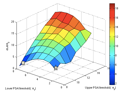
Figure 2: Sensitivity of $\tilde{\theta}_{3}$ as a function of the values of $\tilde{\theta}_{1}$ and $\tilde{\theta}_{2}$ (Patient #15)

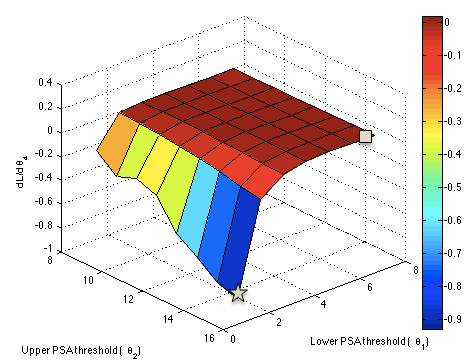
Figure 3: Sensitivity of $\tilde{\theta}_{4}$ as a function of the values of $\tilde{\theta}_{1}$ and $\tilde{\theta}_{2}$ (Patient #15)

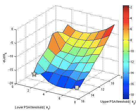
Figure 4: Sensitivity of $\tilde{\theta}_{5}$ as a function of the values of $\tilde{\theta}_{1}$ and $\tilde{\theta}_{2}$ (Patient #15)

Figure 5: Sensitivity of $\tilde{\theta}_{6}$ as a function of the values of $\tilde{\theta}_{1}$ and $\tilde{\theta}_{2}$ (Patient #15)

Figs. 6-9 show how the values of the sensitivities, $\frac{dL}{d\tilde{\theta}_{i}}$, $i=3,\ldots,6$, vary as a function of the values of the lower and upper PSA thresholds ($\frac{dL}{d\tilde{\theta}_{1}}$ and $\frac{dL}{d\tilde{\theta}_{2}}$, respectively) for the model of Patient #1.

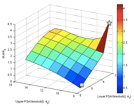
Figure 6: Sensitivity of $\tilde{\theta}_{3}$ as a function of the values of $\tilde{\theta}_{1}$ and $\tilde{\theta}_{2}$ (Patient #1)

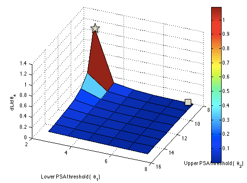
Figure 7: Sensitivity of $\tilde{\theta}_{4}$ as a function of the values of $\tilde{\theta}_{1}$ and $\tilde{\theta}_{2}$ (Patient #1)

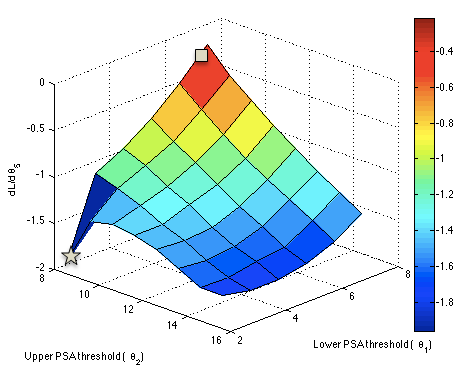
Figure 8: Sensitivity of $\tilde{\theta}_{5}$ as a function of the values of $\tilde{\theta}_{1}$ and $\tilde{\theta}_{2}$ (Patient #1)

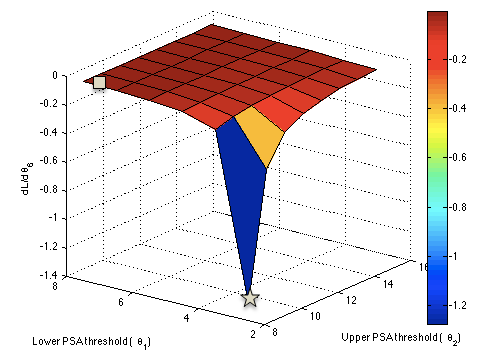
Figure 9: Sensitivity of $\tilde{\theta}_{6}$ as a function of the values of $\tilde{\theta}_{1}$ and $\tilde{\theta}_{2}$ (Patient #1)

The above results lend themselves to the following discussion: first, the values of the model parameter sensitivities, $\frac{dL}{d\tilde{\theta}_{i}}$, $i=3,\ldots,6$, are neither monotonically increasing nor monotonically decreasing along the allowable ranges of $\frac{dL}{d\tilde{\theta}_{1}}$ and $\frac{dL}{d\tilde{\theta}_{2}}$; this is verified for both patients. Second, the system is more sensitive to parameters $\tilde{\theta}_{3}$ and $\tilde{\theta}_{5}$ (HSC proliferation and apoptosis constants, respectively), and more robust to $\tilde{\theta}_{4}$ and $\tilde{\theta}_{6}$ (CRC proliferation and apoptosis constants, respectively); again this is verified across different patients. A possible explanation for this has to do with the fact that HSCs are commonly assumed to be the dominant subpopulation is a prostate tumor undergoing IAS therapy, which means that the size of the this subpopulation has a greater impact on the overall size of the tumor and, consequently, on the value of the PSA level.

Additionally, note that two points are marked in Figs. 2-9: a star marks the optimal therapy configuration and a square marks the values of $\tilde{\theta}_{1}$ and $\tilde{\theta}_{2}$ for which the sensitivities $\frac{dL}{d\tilde{\theta}_{i}}$, $i=3,\ldots,6$, are minimal. In [6] the optimal therapy configurations were found to be $\left[\tilde{\theta}_{1}^{\ast},\tilde{\theta}_{2}^{\ast}\right]=\left[1.5,8.0\right]$ for Patient #15 and $\left[\tilde{\theta}_{1}^{\ast},\tilde{\theta}_{2}^{\ast}\right]=\left[2.5,8.0\right]$ for Patient #1. As it can be seen in Figs. 2-9, these settings are not located in the regions of minimum sensitivities. Of note, the sensitivities $\frac{dL}{d\tilde{\theta}_{i}}$, $i=3,\ldots,6$, take their minimum value at the same suboptimal configuration (namely $\left[\tilde{\theta}_{1},\tilde{\theta}_{2}\right]=\left[7.5,8.0\right]$) across different patients. This could potentially point to the existence of an underlying, and most likely as of yet poorly understood, equilibrium of cancer cell subpopulation dynamics at this suboptimal setting.

Moreover, the tradeoff between system fragility and optimality seems more strongly applicable to $\tilde{\theta}_{1}$, and less so to $\tilde{\theta}_{2}$; interestingly, the value of $\tilde{\theta}_{1}^{\ast}$ differed across patients, while $\tilde{\theta}_{2}^{\ast}$ did not. In this sense, relaxing the optimality condition in favor of increased system robustness could potentially be worthwhile in at least some cases. In fact, for Patient #1, moving from an optimal therapy setting to a slightly suboptimal setting along $\tilde{\theta}_{2}$ (namely $\left[\tilde{\theta}_{1},\tilde{\theta}_{2}\right]=\left[2.5,9.0\right]$) leads to a 9% increase in the cost of treatment. However, the model parameter sensitivities at this setting decrease by approximately 30% for $\tilde{\theta}_{3}$ and $\tilde{\theta}_{5}$ and by approximately 70% for $\tilde{\theta}_{4}$ and $\tilde{\theta}_{6}$. If we move to a suboptimal setting along $\tilde{\theta}_{1}$ (namely $\left[\tilde{\theta}_{1},\tilde{\theta}_{2}\right]=\left[3.5,8.0\right]$), the cost increases by 16%, while the sensitivities decrease by approximately 50% for $\tilde{\theta}_{3}$ and $\tilde{\theta}_{5}$ and by approximately 90% for $\tilde{\theta}_{4}$ and $\tilde{\theta}_{6}$. In this case, it seems advantageous to tradeoff optimality for increased robustness.

It is interesting to note that the above analysis is not consistently verified across different patients. In fact, for Patient #15, a marked decrease in system fragility only occurs when we move to a suboptimal setting along $\tilde{\theta}_{1}$ (namely $\left[\tilde{\theta}_{1},\tilde{\theta}_{2}\right]=\left[7.5,8.0\right]$), at which point the sensitivities decrease by approximately 70% for $\tilde{\theta}_{3}$ and $\tilde{\theta}_{5}$ and by approximately 99% for $\tilde{\theta}_{4}$ and $\tilde{\theta}_{6}$. However, there is an increase in the cost value of the order of 70%, which indicates that system optimality is significantly compromised. These results highlight the importance of applying our methodology on a patient-by-patient basis. More generally, they validate recent efforts favoring the development of personalized cancer therapies, as opposed to traditional treatment schemes that are typically generated over a cohort of patients and thus effective only on average.

V Conclusions

We use a stochastic model of prostate cancer evolution under IAS therapy to perform sensitivity analysis with respect to several important model parameters. We find the system to be more sensitive to changes in the HSC proliferation and apoptosis constants than changes in the CRC proliferation and apoptosis constants. We also identify a set of model parameter values for which the simulated IAS therapy scheme is essentially curative, as well as a set of model parameters for which the prostate tumor grows in an uncontrollable manner. Finally, we verify that relaxing optimality in favor of increased system stability can potentially be of interest in at least some cases.

This work is a first attempt at investigating the tradeoff between optimality and system robustness/fragility in stochastic models of cancer evolution. A subset of all model parameters is selected and a case study of prostate cancer is used to illustrate the applicability of our IPA-based methodology. Nevertheless, there exist several other potentially critical parameters in the SHA model of prostate cancer evolution we study, so that part of our ongoing work includes extending this sensitivity analysis study to other model parameters. Additionally, future work includes applying this methodology to other types of cancer (e.g., breast cancer), as well as other diseases that are known to progress in stages (e.g., tuberculosis).

References

- [1] N. Bruchovsky, L. Klotz, J. Crook, S. Malone, C. Ludgte, W. Morris, M.E. Gleave, S.L. Goldenberg, and P.S. Rennie. Final results of the Canadian prospective phase II trial of intermittent androgen suppression for men in biochemical recurrence after radiotherapy for locally advanced prostate cancer. Cancer, 107:389–395, 2006.
- [2] N. Bruchovsky, L. Klotz, J. Crook, S. Malone, C. Ludgte, W. Morris, M.E. Gleave, S.L. Goldenberg, and P.S. Rennie. Locally advanced prostate cancer biochemical results from a prospective phase II study of intermittent androgen suppression for men with evidence of prostate-specific antigen recurrence after radiotherapy. Cancer, 109:858–867, 2007.
- [3] C.G. Cassandras and S. Lafortune. Introduction to Discrete Event Systems. Springer, 2nd edition, 2008.
- [4] C.G. Cassandras, Y. Wardi, C.G. Panayiotou, and C. Yao. Perturbation analysis and optimization of stochastic hybrid systems. European Journal of Control, 6(6):642–664, 2010.
- [5] J. L. Fleck and C. G. Cassandras. Infinitesimal perturbation analysis for personalized cancer therapy design. Proc. of 5th IFAC Conference on Analysis and Design of Hybrid Systems, pages 205–210, 2015.
- [6] J. L. Fleck and C. G. Cassandras. Optimal design of personalized prostate cancer therapy using infinitesimal perturbation analysis. Nonlinear Analysis: Hybrid Systems, under review.
- [7] Y. Hirata, N. Bruchovsky, and K. Aihara. Development of a mathematical model that predicts the outcome of hormone therapy for prostate cancer. J. Theor. Biology, 264:517–527, 2010.
- [8] Y. Hirata, M. di Bernardo, N. Bruchovsky, and K. Aihara. Hybrid optimal scheduling for intermittent androgen suppression of prostate cancer. Chaos, 20:045125, 2010.
- [9] A.M. Ideta, G. Tanaka, T. Takeuchi, and K. Aihara. A mathematical model for intermittent androgen suppression for prostate cancer. J. Nonlinear Sci., 18:593–614, 2008.
- [10] T.L. Jackson. A mathematical investigation of the multiple pathways to recurrent prostate cancer: comparison with experimental data. Neoplasia, 6:697–704, 2004.
- [11] B. Liu, S. Kong, S. Gao, P. Zuliani, and E.M. Clarke. Towards personalized cancer therapy using delta-reachability analysis. HSCC2015, 2015.
- [12] D.L. Longo, A.S. Fauci, D.L. Kasper, S.L. Hauser, J.L. Jameson, and J. Loscalzo, editors. Harrison’s principles of internal medicine. McGraw-Hill, Medical Pub. Division, New York, 18th edition, 2012.
- [13] T. Shimada and K. Aihara. A nonlinear model with competition between prostate tumor cells and its application to intermittent androgen suppression therapy of prostate cancer. Mathematical Biosciences, 214:134–139, 2008.
- [14] T. Suzuki, N. Bruchovsky, and K. Aihara. Piecewise affine systems modelling for optimizing therapy of prostate cancer. Philos. Trans. R. Soc., 368:5045–5059, 2010.
- [15] G. Tanaka, Y. Hirata, S.L. Goldenberg, N. Bruchovsky, and K. Aihara. Mathematical modelling of prostate cancer growth and its application to hormone therapy. Philos. Trans. R. Soc., 368:5029–5044, 2010.
- [16] Y. Tao, Q. Guo, and K. Aihara. A mathematical model of prostate tumor growth under hormone therapy with mutation inhibitor. J. Nonlinear Sci., 20:219–240, 2010.