Optimization via Chebyshev Polynomials

Abstract

This paper presents for the first time a robust exact line-search method based on a full pseudospectral (PS) numerical scheme employing orthogonal polynomials. The proposed method takes on an adaptive search procedure and combines the superior accuracy of Chebyshev PS approximations with the high-order approximations obtained through Chebyshev PS differentiation matrices (CPSDMs). In addition, the method exhibits quadratic convergence rate by enforcing an adaptive Newton search iterative scheme. A rigorous error analysis of the proposed method is presented along with a detailed set of pseudocodes for the established computational algorithms. Several numerical experiments are conducted on one- and multi-dimensional optimization test problems to illustrate the advantages of the proposed strategy.

1 Introduction

The area of optimization received enormous attention in recent years due to the rapid progress in computer technology, development of user-friendly software, the advances in scientific computing provided, and most of all, the remarkable interference of mathematical programming in crucial decision-making problems. One-dimensional optimization or simply line search optimization is a branch of optimization that is most indispensable, as it forms the backbone of nonlinear programming algorithms. In particular, it is typical to perform line search optimization in each stage of multivariate algorithms to determine the best length along a certain search direction; thus, the efficiency of multivariate algorithms largely depends on it. Even in constructing high-order numerical quadratures, line search optimization emerges in minimizing their truncation errors; thus boosting their accuracy and allowing to obtain very accurate solutions to intricate boundary-value problems, integral equations, integro-differential equations, and optimal control problems in short times via stable and efficient numerical schemes; cf. [Elgindy et al (2012), Elgindy and Smith-Miles (2013), Elgindy and Smith-Miles (2013a), Elgindy and Smith-Miles (2013b), Elgindy (2016a), Elgindy (2016b)].

Many line search methods were presented in the literature in the past decades. Some of the most popular line search methods include interpolation methods, Fibonacci’s method, golden section search method, secant method, Newton’s method, to mention a few; cf. [Pedregal (2006), Chong and Zak (2013), Nocedal and Wright (2006)]. Perhaps Brent’s method is considered one of the most popular and widely used line search methods nowadays. It is a robust version of the inverse parabolic interpolation method that makes the best use of both techniques, the inverse parabolic interpolation method and the golden section search method, and can be implemented in MATLAB software, for instance, using the ‘fminbnd’ optimization solver. The method is a robust optimization algorithm that does not require derivatives; yet it lacks the rapid convergence rate manifested in the derivative methods when they generally converge.

In $2008$, [Elgindy and Hedar (2008)] gave a new approach for constructing an exact line search method using Chebyshev polynomials, which have become increasingly important in scientific computing, from both theoretical and practical points of view. They introduced a fast line search method that is an adaptive version of Newton’s method. In particular, their method forces Newton’s iterative scheme to progress only in descent directions. Moreover, the method replaces the classical finite-difference formulas for approximating the derivatives of the objective function by the more accurate step lengths along the Chebyshev pseudospectral (PS) differentiation matrices (CPSDMs); thus getting rid of the dependency of the iterative scheme on the choice of the step-size, which can significantly affect the quality of calculated derivatives approximations. Although the method worked quite well on some test functions, where classical Newton’s method fail to converge, the method may still suffer from some drawbacks that we discuss thoroughly later in the next section.

In this article, the question of how to construct an exact line search method based on PS methods is re-investigated and explored. We present for the first time a robust exact line-search method based on a full PS numerical scheme employing Chebyshev polynomials and adopting two global strategies: (i) Approximating the objective function by an accurate fourth-order Chebyshev interpolant based on Chebyshev-Gauss-Lobatto (CGL) points; (ii) approximating the derivatives of the function using CPSDMs. The first strategy actually plays a significant role in capturing a close profile to the objective function from which we can determine a close initial guess to the local minimum, since Chebyshev polynomials as basis functions can represent smooth functions to arbitrarily high accuracy by retaining a finite number of terms. This approach also improves the performance of the adaptive Newton’s iterative scheme by starting from a sufficiently close estimate; thus moving in a quadratic convergence rate. The second strategy yields accurate search directions by maintaining very accurate derivative approximations. The proposed method is also adaptive in the sense of searching only along descent directions, and avoids the raised drawbacks pertaining to the [Elgindy and Hedar (2008)] method.

The rest of the article is organized as follows: In the next section, we revisit the [Elgindy and Hedar (2008)] method highlighting its strengths aspects and weaknesses. In Section 3, we provide a modified explicit expression for higher-order CPSDMs based on the successive differentiation of the Chebyshev interpolant. We present the novel line search strategy in Section 4 using first-order and/or second-order information, and discuss its integration with multivariate nonlinear optimization algorithms in Section 4.3. Furthermore, we provide a rigorous error and sensitivity analysis in Sections 5 and 6, respectively. Section 7 verifies the accuracy and efficiency of the proposed method through an extensive sets of one- and multi-dimensional optimization test examples followed by some conclusions given in Section 8. Some useful background in addition to some useful pseudocodes for implementing the developed method are presented in Appendices A and B, respectively.

2 The [Elgindy and Hedar (2008)] Optimization Method Revisited

The [Elgindy and Hedar (2008)] line search method is an adaptive method that is considered an improvement over the standard Newton’s method and the secant method by forcing the iterative scheme to move in descent directions. The developed algorithm is considered unique as it exploits the peculiar convergence properties of spectral methods, the robustness of orthogonal polynomials, and the concept of PS differentiation matrices for the first time in a one-dimensional search optimization. In addition, the method avoids the use of classical finite difference formulas for approximating the derivatives of the objective function, which are often sensitive to the values of the step-size.

The success in carrying out the above technique lies very much in the linearity property of the interpolation, differentiation, and evaluation operations. Indeed, since all of these operations are linear, the process of obtaining approximations to the values of the derivative of a function at the interpolation points can be expressed as a matrix-vector multiplication. In particular, if we approximate the derivatives of a function $f(x)$ by interpolating the function with an $n$th-degree polynomial $P_{n}(x)$ at, say, the CGL points defined by Eq. (A.7), then the values of the derivative $P^{\prime}_{n}(x)$ at the same $(n+1)$ points can be expressed as a fixed linear combination of the given function values, and the whole relationship can be written in the following matrix form:

$$\left({\begin{array}[]{*{20}{l}}{{P^{\prime}_{n}}({x_{0}})}\\ {\,\,\quad\vdots}\\ {{P^{\prime}_{n}}({x_{n}})}\end{array}}\right)=\left({\begin{array}[]{*{20}{c}}{d_{00}^{(1)}}&\ldots&{d_{0n}^{(1)}}\\ \vdots&\ddots&\vdots\\ {d_{n0}^{(1)}}&\cdots&{d_{nn}^{(1)}}\end{array}}\right)\left({\begin{array}[]{*{20}{l}}{f({x_{0}})}\\ {\quad\,\vdots}\\ {f({x_{n}})}\end{array}}\right).$$ (2.1)

Setting $\bm{\mathcal{F}}=[f(x_{0}),f(x_{1}),\ldots,f(x_{n})]^{T}$, as the vector consisting of values of $f(x)$ at the $(n+1)$ interpolation points, $\bm{\Psi}=[P^{\prime}_{n}(x_{0}),P^{\prime}_{n}(x_{1}),\ldots,P^{\prime}_{n}(x_{n})]^{T}$, as the values of the derivative at the CGL points, and $\bm{D}^{(1)}=(d_{ij}^{(1)})\;,\;0\leq i,j\leq n$, as the first-order differentiation matrix mapping $\bm{\mathcal{F}}\to\bm{\Psi}$, then Formula (2.1) can be written in the following simple form

$$\bm{\Psi}=\bm{D}^{(1)}\bm{\mathcal{F}}.$$ (2.2)

Eq. (2.2) is generally known as the PS differentiation rule, and it generally delivers better accuracy than standard finite-difference rules. We show later in the next section some modified formulas for calculating the elements of a general $q$th-order CPSDM, $\bm{D}^{(q)}\;\forall q\geq 1$. Further information on classical explicit expressions of the entries of differentiation matrices can be found in [Weideman and Reddy (2000), Baltensperger (2000), Costa and Don (2000), Elbarbary and El-Sayed (2005)].

A schematic figure showing the framework of [Elgindy and Hedar (2008)] line search method is shown in Figure 1. As can be observed from the figure, the method starts by transforming the uncertainty interval $[a,b]$ into the domain $[-1,1]$ to exploit the rapid convergence properties provided by Chebyshev polynomials. The method then takes on a global approach in calculating the derivatives of the function at the CGL points, $\{x_{i}\}_{i=0}^{n}$, using CPSDMs. If the optimality conditions are not satisfied at any of these candidate points, the method then endeavors to locate the best point $x_{m}$ that minimizes the function, and decides whether to keep or expand the uncertainty interval. An update $\tilde{x}_{m}$ is then calculated using the descent direction property followed by updating row $m$ in both matrices $\bm{D}^{(1)}$ and $\bm{D}^{(2)}$. The iterative scheme proceeds repeatedly until the stopping criterion is satisfied.

Although the method possesses many useful features over classical Newton’s method and the secant method; cf. [Elgindy and Hedar (2008), Section 8], it may still suffer from the following drawbacks: (i) In spite of the fact that, $\bm{D}^{(1)}$ and $\bm{D}^{(2)}$ are constant matrices, the method requires the calculation of their entire elements beforehand. We show later that we can establish rapid convergence rates using only one row from each matrix in each iterate. (ii) The method attempts to calculate the first and second derivatives of the function at each point $x_{i}\in[-1,1],i=0,\ldots,n$. This could be expensive for large values of $n$, especially if the local minimum $t^{*}$ is located outside the initial uncertainty interval $[a,b]$; cf. [Elgindy and Hedar (2008), Table 6], for instance. (iii) The method takes on a global approach for approximating the derivatives of the objective function using CPSDMs instead of the usual finite-difference formulas that are highly sensitive to the values of the step-size. However, the method locates a starting approximation by distributing the CGL points along the interval $[-1,1]$, and finding the point that best minimizes the value of the function among all other candidate points. We show later in Section 4 that we can significantly speed up this process by adopting another global approach based on approximating the function via a fourth-order Chebyshev interpolant, and determining the starting approximation through finding the best root of the interpolant derivative using exact formulas. (iv) During the implementation of the method, the new approximation to the local minimum, $\tilde{x}_{m}$, may lie outside the interval $[-1,1]$ in some unpleasant occasions; thus the updated differentiation matrices may produce false approximations to the derivatives of the objective function. (v) To maintain the adaptivity of the method, the authors proposed to flip the sign of the second derivative $f^{\prime\prime}$ whenever $f^{\prime\prime}<0$, at some point followed by its multiplication with a random positive number $\beta$. This operation may not be convenient in practice; therefore, we need a more efficient approach to overcome this difficulty. (vi) Even if $f^{\prime\prime}>0$, at some point, the magnitudes of $f^{\prime}$ and $f^{\prime\prime}$ may be too small slowing down the convergence rate of the method. This could happen for instance if the function has a multiple local minimum, or has a nearly flat profile about $t^{*}$. (vii) Suppose that $t^{*}$ belongs to one side of the real line while the initial search interval $[a,b]$ is on the other side. According to the presented method, the search interval must shrink until it converges to the point zero, and the search procedure halts. Such drawbacks motivate us to develop a more robust and efficient line search method.

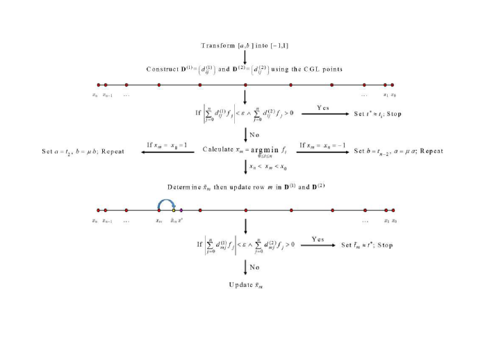
Figure 1: An illustrative figure showing the framework of the line search method introduced by [Elgindy and Hedar (2008)] for minimizing a single-variable function $f:[a,b]\to\mathbb{R}$, where $\{x_{i}\}_{i=0}^{n}$ are the CGL points, $t_{i}=\left((b-a)x_{i}+a+b\right)/2\;\forall i$, are the corresponding points in $[a,b]$, $f_{i}=f(t_{i})\;\forall i$, $\varepsilon$ is a relatively small positive number, $\mu>1$, is a parameter preferably chosen as $1.618^{k}$, where $\rho\approx 1.618$ is the golden ratio, and $k=1,2,\ldots$, is the iteration counter

3 High-Order CPSDMs

In the sequel, we derive a modified explicit expression for higher-order CPSDMs to that stated in [Elgindy and Hedar (2008)] based on the successive differentiation of the Chebyshev interpolant. The higher derivatives of Chebyshev polynomials are expressed in standard polynomial form rather than as Chebyshev polynomial series expansion. The relation between Chebyshev polynomials and trigonometric functions is used to simplify the expressions obtained, and the periodicity of the cosine function is used to express it in terms of existing nodes.

The following theorem gives rise to a modified useful form for evaluating the $m$th-derivative of Chebyshev polynomials.

Theorem 3.1.

The $m$th-derivative of the Chebyshev polynomials is given by

$$0,\quad 0\leq k<m,$$ (3.1a)

$$1,\quad k=m=0,$$ (3.1b)

$${2^{k-1}}m!,\quad k=m\geq 1,$$ (3.1c)

$$\sum\limits_{l=0}^{\left\lfloor k/2\right\rfloor}{\gamma_{l,k}^{(m)}\,c_{l}^{(k)}{x^{k-2l-m}}},\quad k>m\geq 0\wedge x\neq 0,$$ (3.1d)

$$\beta_{k}^{(m)}\cos\left({\frac{\pi}{2}\left({k-{\delta_{\frac{{m+1}}{2},\left\lfloor{\frac{{m+1}}{2}}\right\rfloor}}}\right)}\right),\quad k>m\geq 0\wedge x=0,$$ (3.1e)

where

$$1,\quad m=0,$$ (3.2a)

$$\left({k-2l-m+1}\right){\left({k-2l-m+2}\right)_{m-1}},\quad m\geq 1,$$ (3.2b)

$$1,\quad l=k=0,$$ (3.3a)

$${2^{k-1}},\quad l=0\wedge k\geq 1,$$ (3.3b)

$$-\frac{{\left({k-2l+1}\right)\left({k-2l+2}\right)}}{{4l\left({k-l}\right)}}c_{l-1}^{(k)},\quad l=1,\ldots,\left\lfloor{k/2}\right\rfloor\wedge k\geq 1,$$ (3.3c)

$$1,\quad m=0,$$ (3.4a)

$${\left({-4}\right)^{\left\lfloor{\frac{{m-1}}{2}}\right\rfloor}}{\left({-1}\right)^{{\delta_{\frac{{m+1}}{2},\left\lfloor{\frac{{m+1}}{2}}\right\rfloor}}+\left\lfloor{\frac{{m+1}}{2}}\right\rfloor}}{k^{{\delta_{\frac{m}{2},\left\lfloor{\frac{m}{2}}\right\rfloor}}+1}}{\left({\frac{1}{2}\left({-k-{\delta_{\frac{{m+1}}{2},\left\lfloor{\frac{{m+1}}{2}}\right\rfloor}}+2}\right)}\right)_{\left\lfloor{\frac{{m-1}}{2}}\right\rfloor}}\times$$

$${\left({\frac{1}{2}\left({k-{\delta_{\frac{{m+1}}{2},\left\lfloor{\frac{{m+1}}{2}}\right\rfloor}}+2}\right)}\right)_{\left\lfloor{\frac{{m-1}}{2}}\right\rfloor}},\quad m\geq 1,$$ (3.4b)

$\left\lfloor x\right\rfloor$ is the floor function of a real number $x$; ${(x)_{l}}=x(x+1)\ldots(x+l-1)$ is the Pochhammer symbol, for all $l\in\mathbb{Z}^{+}$.

Proof.

The proof of Eqs. (3.1a)-(3.1c) is straightforward using Eqs. (A.1)-(A.3). We prove Eqs. (3.1d) and (3.1e) by mathematical induction. So consider the case where $k>m\geq 0\wedge x\neq 0$. For $m=0$, we can rewrite Eq. (A.2) with a bit of manipulation in the form

$${T_{k}}(x)=\sum\limits_{l=0}^{\left\lfloor{k/2}\right\rfloor}{c_{l}^{(k)}{x^{k-2l}}}.$$ (3.5)

For $m=1$, we have

$$\sum\limits_{l=0}^{\left\lfloor{k/2}\right\rfloor}{\gamma_{l,k}^{(1)}{\mkern 1.0mu}{\kern 1.0pt}c_{l}^{(k)}{x^{k-2l-1}}}=\sum\limits_{l=0}^{\left\lfloor{k/2}\right\rfloor}{(k-2l)c_{l}^{(k)}{x^{k-2l-1}}}=\frac{d}{{dx}}\sum\limits_{l=0}^{\left\lfloor{k/2}\right\rfloor}{c_{l}^{(k)}{x^{k-2l}}}={T^{\prime}_{k}}(x),$$

so the theorem is true for $m=0$ and $1$. Now, assume that the theorem is true for $m=n$, then for $m=n+1$, we have

$$\sum\limits_{l=0}^{\left\lfloor{k/2}\right\rfloor}{\gamma_{l,k}^{(n+1)}\,c_{l}^{(k)}{x^{k-2l-n-1}}}=\sum\limits_{l=0}^{\left\lfloor{k/2}\right\rfloor}{(k-2l-n)\,\gamma_{l,k}^{(n)}\,c_{l}^{(k)}{x^{k-2l-n-1}}}=\frac{d}{{dx}}\sum\limits_{l=0}^{\left\lfloor{k/2}\right\rfloor}{\gamma_{l,k}^{(n)}\,c_{l}^{(k)}{x^{k-2l-n}}}=T_{k}^{(n+1)}(x).$$

Hence Eq. (3.1d) is true for every positive integer $m$. Now consider the case $k>m\geq 0\wedge x=0$. The proof of Eq. (3.1e) for $m=0$ is trivial, so consider the case $m=1$, where the proof is derived as follows:

$$\beta_{k}^{(1)}\cos\left({\frac{\pi}{2}(k-1)}\right)={(-1)^{2}}k\cos\left({\frac{\pi}{2}(k-1)}\right)=k\sin\left({\frac{{k\pi}}{2}}\right)={T^{\prime}_{k}}(0).$$

Now assume that Eq. (3.1e) is true for $m=n$. We show that it is also true for $m=n+1$. Since

$$T_{k}^{(n+1)}(x)=\frac{{{d^{n}}}}{{d{x^{n}}}}{{T^{\prime}}_{k}}(x),$$ (3.6)

then substituting Eq. (A.8) in Eq. (3.6) yields

$$T_{k}^{(n+1)}(x)=\frac{k}{2}\frac{{{d^{n}}}}{{d{x^{n}}}}(\phi(x)\;\psi(x)),$$ (3.7)

where $\phi(x)={T_{k-1}}(x)-{T_{k+1}}(x)\;;\;\psi(x)=1/(1-{x^{2}})$. Since

$${\psi^{(n)}}(0)=\left\{{\begin{array}[]{*{20}{l}}{0,\quad n\;{\text{is odd}},}\\ {n!,\quad n\;{\text{is even}},}\end{array}}\right.$$ (3.8)

then by the general Leibniz rule,

$${(\phi(x)\cdot\psi(x))^{(n)}}=\sum\limits_{k=0}^{n}{\left(\begin{array}[]{c}n\\ k\end{array}\right)}\,{\phi^{(n-k)}}(x)\,{\psi^{(k)}}(x),$$ (3.9)

Eq. (3.7) at $x=0$ is reduced to

$$T_{k}^{(n+1)}(0) =\frac{k}{2}\sum\limits_{\scriptstyle l=0\atop\scriptstyle l\;{\text{is even}}}^{n}{\left({\begin{array}[]{*{20}{l}}n\\ l\end{array}}\right)\,{\phi^{(n-l)}}(0)\,{\psi^{(l)}}(0)}=\frac{1}{2}\,k\cdot n!\;\sum\limits_{\scriptstyle l=0\atop\scriptstyle l\;{\text{is even}}}^{n}{\frac{{{\phi^{(n-l)}}(0)}}{{(n-l)!}}}=\frac{1}{2}\,k\cdot n!\;\sum\limits_{\scriptstyle l=0\atop\scriptstyle l\;{\text{is even}}}^{n}{\frac{1}{{(n-l)!}}\left({T_{k-1}^{(n-l)}(0)-T_{k+1}^{(n-l)}(0)}\right)}$$

$$=\frac{1}{2}\,k\cdot n!\;\sum\limits_{\scriptstyle l=0\atop\scriptstyle l\;{\text{is even}}}^{n}{\frac{1}{{(n-l)!}}\left({\beta_{k-1}^{(n-l)}\cos\left({\frac{\pi}{2}\left({k-1-{\delta_{\frac{{n-l+1}}{2},\left\lfloor{\frac{{n-l+1}}{2}}\right\rfloor}}}\right)}\right)-\beta_{k+1}^{(n-l)}\cos\left({\frac{\pi}{2}\left({k+1-{\delta_{\frac{{n-l+1}}{2},\left\lfloor{\frac{{n-l+1}}{2}}\right\rfloor}}}\right)}\right)}\right)}$$

$$=\beta_{k}^{(n+1)}\cos\left({\frac{\pi}{2}\left({k-{\delta_{\frac{{n+2}}{2},[\frac{{n+2}}{2}]}}}\right)}\right),$$

which completes the proof. ∎

Introducing the parameters,

$${\theta_{j}}=\left\{\begin{array}[]{l}1/2,\quad j=0,n,\\ 1,\quad j=1,\ldots,n-1,\end{array}\right.$$ (3.10)

replaces formulas (A.9) and (A.10) with

$$P_{n}(x)=\sum\limits_{k=0}^{n}{\theta_{k}a_{k}T_{k}(x)},$$ (3.11)

$$a_{k}=\frac{2}{n}\sum\limits_{j=0}^{n}{\theta_{j}f_{j}T_{k}(x_{j})},$$ (3.12)

where $f_{j}={f({x_{j}})}\;\forall j$. Substituting Eq. (3.12) into Eq. (3.11) yields

$$P_{n}(x)=\frac{2}{n}\sum\limits_{k=0}^{n}{\sum\limits_{j=0}^{n}{\theta_{j}\theta_{k}f_{j}T_{k}(x_{j})T_{k}(x)}}.$$ (3.13)

The derivatives of the Chebyshev interpolant $P_{n}(x)$ of any order $m$ are then computed at the CGL points by differentiating (3.13) such that

$$P_{n}^{(m)}(x_{i})=\frac{2}{n}\sum\limits_{j=0}^{n}\sum\limits_{k=0}^{n}\theta_{j}\theta_{k}f_{j}T_{k}(x_{j})T_{k}^{(m)}(x_{i})=\sum\limits_{j=0}^{n}{d_{ij}^{(m)}f_{j}},\quad m\geq 0,$$ (3.14)

where

$$d_{ij}^{(m)}={\frac{2\theta_{j}}{n}\sum\limits_{k=0}^{n}\theta_{k}T_{k}(x_{j})T_{k}^{(m)}(x_{i})},$$ (3.15)

are the elements of the $m$th-order CPSDM. With the aid of Theorem 3.1, we can now calculate the elements of the $m$th-order CPSDM using the following useful formula:

$$d_{ij}^{(m)} =\frac{2{\theta_{j}}}{n}\mathop{\sum}\limits_{k=m}^{n}{\theta_{k}}{T_{k}}({x_{j}})\left({\left\{\begin{array}[]{l}1,\quad k=m=0,\\ {2^{k-1}}m!,\quad k=m\geq 1,\\ \mathop{\sum}\limits_{l=0}^{\left\lfloor{k/2}\right\rfloor}c_{l}^{(k)}\,\gamma_{l,k}^{(m)}\,x_{i}^{k-2l-m},\quad k>m\geq 0\wedge{x_{i}}\neq 0,\\ \beta_{k}^{(m)}\cos\left({\frac{\pi}{2}\left({k-{\delta_{\frac{{m+1}}{2},\lfloor\frac{{m+1}}{2}\rfloor}}}\right)}\right),\quad k>m\geq 0\wedge{x_{i}}=0\end{array}\right.}\right)$$ (3.16e)

$$=\frac{2{\theta_{j}}}{n}\mathop{\sum}\limits_{k=m}^{n}{\theta_{k}}{T_{k}}({x_{j}})\left({\left\{\begin{array}[]{l}1,\quad k=m=0,\\ {2^{k-1}}m!,\quad k=m\geq 1,\\ \mathop{\sum}\limits_{l=0}^{\left\lfloor{k/2}\right\rfloor}c_{l}^{(k)}\,\gamma_{l,k}^{(m)}\,x_{i}^{k-2l-m},\quad k>m\geq 0\wedge i\neq\frac{n}{2},\\ \beta_{k}^{(m)}\cos\left({\frac{\pi}{2}\left({k-{\delta_{\frac{{m+1}}{2},\lfloor\frac{{m+1}}{2}\rfloor}}}\right)}\right),\quad k>m\geq 0\wedge i=\frac{n}{2}\end{array}\right.}\right).$$ (3.16j)

Using the following periodic property of the cosine function

$$\cos\left({\pi x}\right)={\left({-1}\right)^{\lfloor x\rfloor}}\cos\left({\pi\left({x-\lfloor x\rfloor}\right)}\right)\;\forall x\in\mathbb{R},$$ (3.17)

we can further rewrite Eqs. (3.16j) as follows:

$$d_{ij}^{(m)}=\frac{2{\theta_{j}}}{n}\mathop{\sum}\limits_{k=m}^{n}{\theta_{k}}{\left({-1}\right)^{\lfloor jk/n\rfloor}}{x_{jk-n{\kern 1.0pt}\left\lfloor{\frac{{jk}}{n}}\right\rfloor}}\left({\left\{\begin{array}[]{l}1,\quad k=m=0,\\ {2^{k-1}}m!,\quad k=m\geq 1,\\ \mathop{\sum}\limits_{l=0}^{\lfloor k/2\rfloor}c_{l}^{(k)}\gamma_{l,k}^{(m)}x_{i}^{k-2l-m},\quad k>m\geq 0\wedge i\neq\frac{n}{2},\\ {\left({-1}\right)^{\lfloor\sigma_{k}^{(m)}\rfloor}}\beta_{k}^{(m)}{x_{n\left({\sigma_{k}^{(m)}-\lfloor\sigma_{k}^{(m)}\rfloor}\right)}},\quad k>m\geq 0\wedge i=\frac{n}{2}\end{array}\right.}\right),$$ (3.18)

where $\sigma_{k}^{(m)}=\left({k-{\delta_{\frac{{1+m}}{2},\left\lfloor{\frac{{1+m}}{2}}\right\rfloor}}}\right)/2$. To improve the accuracy of Eqs. (3.18), we can use the negative sum trick, computing all the off-diagonal elements then applying the formula

$$d_{ii}^{(m)}=-\sum\limits_{\scriptstyle j=0\hfill\atop\scriptstyle j\neq i\hfill}^{n}{d_{ij}^{(m)}}\quad\forall m\geq 1,$$ (3.19)

to compute the diagonal elements. Applying the last trick gives the formula

$$d_{ij}^{(m)}=\left\{\begin{array}[]{l}\frac{{2{\theta_{j}}}}{n}\sum\limits_{k=m}^{n}{{\theta_{k}}}{\left({-1}\right)^{\lfloor jk/n\rfloor}}{x_{jk-n\,\left\lfloor{\frac{{jk}}{n}}\right\rfloor}}\left({\left\{\begin{array}[]{l}1,\quad k=m=0\wedge i\neq j,\\ {2^{k-1}}m!,\quad k=m\geq 1\wedge i\neq j,\\ \sum\limits_{l=0}^{\lfloor k/2\rfloor}{c_{l}^{(k)}}\gamma_{l,k}^{(m)}x_{i}^{k-2l-m},\quad k>m\geq 0\wedge i\neq\frac{n}{2}\wedge i\neq j,\\ {\left({-1}\right)^{\lfloor\sigma_{k}^{(m)}\rfloor}}\beta_{k}^{(m)}{x_{n\left({\sigma_{k}^{(m)}-\lfloor\sigma_{k}^{(m)}\rfloor}\right)}},\quad k>m\geq 0\wedge i=\frac{n}{2}\wedge i\neq j,\end{array}\right.}\right)\\ -\sum\nolimits_{\scriptstyle s=0\hfill\atop\scriptstyle s\neq i\hfill}^{n}{d_{is}^{(m)}},\quad i=j\end{array}\right..$$ (3.20)

Hence, the elements of the first- and second-order CPSDMs are given by

$$d_{ij}^{(1)}=\left\{\begin{array}[]{l}\frac{{2{\theta_{j}}}}{n}\sum\limits_{k=1}^{n}{{\theta_{k}}}{\left({-1}\right)^{\lfloor jk/n\rfloor}}{x_{jk-n\,\left\lfloor{\frac{{jk}}{n}}\right\rfloor}}\left({\left\{\begin{array}[]{l}1,\quad k=1\wedge i\neq j,\\ \sum\limits_{l=0}^{\lfloor k/2\rfloor}{\left({k-2l}\right)}\,c_{l}^{(k)}x_{i}^{k-2l-1},\quad k>1\wedge i\neq\frac{n}{2}\wedge i\neq j,\\ {\left({-1}\right)^{\lfloor\frac{{k-1}}{2}\rfloor}}k{\mkern 1.0mu}{x_{n\left({\frac{{k-1}}{2}-\lfloor\frac{{k-1}}{2}\rfloor}\right)}},\quad k>1\wedge i=\frac{n}{2}\wedge i\neq j,\end{array}\right.}\right)\\ -\sum\nolimits_{\scriptstyle s=0\hfill\atop\scriptstyle s\neq i\hfill}^{n}{d_{is}^{(1)}},\quad i=j\end{array}\right.,$$ (3.21)

$$d_{ij}^{(2)}=\left\{\begin{array}[]{l}\frac{{2{\theta_{j}}}}{n}\sum\limits_{k=2}^{n}{{\theta_{k}}}{\left({-1}\right)^{\lfloor jk/n\rfloor}}{x_{jk-n\,\left\lfloor{\frac{{jk}}{n}}\right\rfloor}}\left({\left\{\begin{array}[]{l}4,\quad k=2\wedge i\neq j,\\ \sum\limits_{l=0}^{\lfloor k/2\rfloor}{\left({k-2l-1}\right)}\left({k-2l}\right)c_{l}^{(k)}x_{i}^{k-2l-2},\quad k>2\wedge i\neq\frac{n}{2}\wedge i\neq j,\\ -{\left({-1}\right)^{\lfloor\frac{k}{2}\rfloor}}{k^{2}}{\mkern 1.0mu}{x_{n\left({\frac{k}{2}-\left\lfloor{\frac{k}{2}}\right\rfloor}\right)}},\quad k>2\wedge i=\frac{n}{2}\wedge i\neq j,\end{array}\right.}\right)\\ -\sum\nolimits_{\scriptstyle s=0\hfill\atop\scriptstyle s\neq i\hfill}^{n}{d_{is}^{(2)}},\quad i=j\end{array}\right.,$$ (3.22)

respectively.

4 Proposed Line Search Method

In this section we present a novel line search method that we shall call the Chebyshev PS line search method (CPSLSM). The key idea behind our new approach is five-fold:

1. express the function as a linear combination of Chebyshev polynomials,

2. find its derivative,

3. find the derivative roots,

4. determine a local minimum in $[-1,1]$, and,

5. finally reverse the change of variables to obtain the approximate local minimum of the original function.

To describe the proposed method, let us denote by $\mathbb{P}_{n}$ the space of polynomials of degree at most $n$, and suppose that we want to find a local minimum $t^{*}$ of a twice-continuously differentiable nonlinear single-variable function $f(t)$ on a fixed interval $[a,b]$ to within a certain accuracy $\varepsilon$. Using the change of variable,

$$x=(2\,t-a-b)/(b-a),$$ (4.1)

we transform the interval $[a,b]$ into $[-1,1]$. We shall refer to a point $x$ corresponding to a candidate local minimum point $t$ according to Eq. (4.1) by the translated candidate local minimum point.

Now let $I_{4}f\in\mathbb{P}_{4}$, be the fourth-degree Chebyshev interpolant of $f$ at the CGL points such that

$$f(x;a,b)\approx{I_{4}}f(x;a,b)=\sum\limits_{k=0}^{4}{{{\tilde{f}}_{k}}\,{T_{k}}(x)}.$$ (4.2)

We can determine the Chebyshev coefficients $\{{{\tilde{f}}_{k}}\}_{k=0}^{4}$ via the discrete Chebyshev transform

$${{\tilde{f}}_{k}} =\frac{1}{{2\,{c_{k}}}}\sum\limits_{j=0}^{4}{\frac{1}{{{c_{j}}}}\cos\left({\frac{{k\,j\,\pi}}{4}}\right)\,{}_{a}^{b}{f_{j}}}$$

$$=\frac{1}{{2\,{c_{k}}}}\left[{\frac{1}{2}\left({{}_{a}^{b}{f_{0}}+{{(-1)}^{k}}\,{}_{a}^{b}{f_{4}}}\right)+\sum\limits_{j=1}^{3}{\frac{1}{{{c_{j}}}}\cos\left({\frac{{k\,j\,\pi}}{4}}\right)\,{}_{a}^{b}{f_{j}}}}\right],$$ (4.3)

where ${}_{a}^{b}{f_{j}}=f({x_{j}};a,b),\;j=0,\ldots,4,$ and

$${c_{k}}=\left\{\begin{array}[]{l}2,\quad k=0,4,\\ 1,\quad k=1,\ldots,3.\end{array}\right.$$ (4.4)

We approximate the derivative of $f$ by the derivative of its interpolant ${I_{4}}f(x;a,b)$,

$${I^{\prime}_{4}}f(x;a,b)=\sum\limits_{k=0}^{4}{\tilde{f}_{k}^{(1)}{\mkern 1.0mu}{T_{k}}(x)},$$ (4.5)

where the coefficients $\left\{\tilde{f}_{k}^{(1)}\right\}_{k=0}^{4}$ are akin to the coefficients of the original function, $\tilde{f}_{k}$, by the following recursion [Kopriva (2009)]

$${\tilde{c}_{k}}\,\tilde{f}_{k}^{(1)}=\tilde{f}_{k+2}^{(1)}+2\,(k+1)\,{\tilde{f}_{k+1}},\quad k\geq 0,$$ (4.6)

$${{\tilde{c}}_{k}}=\;\left\{{\begin{array}[]{*{20}{l}}{{c_{k}},\quad k=0,\ldots,3,}\\ {1,\quad k=4.}\end{array}}\right.$$ (4.7)

We can calculate $\left\{\tilde{f}_{k}^{(1)}\right\}_{k=0}^{4}$ efficiently using Algorithm 2. Now we collect the terms involving the same powers of $x$ in Eq. (4.5) to get the cubic algebraic equation

$${I^{\prime}_{4}}f(x;a,b)={A_{1}}{\mkern 1.0mu}{x^{3}}+{A_{2}}{\mkern 1.0mu}{x^{2}}+{A_{3}}{\mkern 1.0mu}x+{A_{4}},$$ (4.8)

where

$${A_{1}} =4{\mkern 1.0mu}\tilde{f}_{3}^{(1)},$$ (4.9a)

$${A_{2}} =2{\mkern 1.0mu}\tilde{f}_{2}^{(1)},$$ (4.9b)

$${A_{3}} =\tilde{f}_{1}^{(1)}-3{\mkern 1.0mu}\tilde{f}_{3}^{(1)},$$ (4.9c)

$${A_{4}} =\tilde{f}_{0}^{(1)}-\tilde{f}_{2}^{(1)}.$$ (4.9d)

Let ${\varepsilon}_{c}$ and $\varepsilon_{\text{mach}}$ denote a relatively small positive number and the machine precision that is approximately equals $2.2204\times 10^{-16}$ in double precision arithmetic, respectively. To find a local minimum of $f$, we consider the following three cases:

Case $\bm{1}$: If $\left|{{A_{1}}}\right|,\left|{{A_{2}}}\right|<{\varepsilon}_{c}$, then ${I^{\prime}_{4}}f(x;a,b)$ is linear or nearly linear. Notice also that $A_{3}$ cannot be zero, since $f$ is nonlinear and formula (4.2) is exact for all polynomials $h_{n}(t)\in\mathbb{P}_{4}$. This motivates us to simply calculate the root $\bar{x}=-{A_{4}}/{A_{3}}$, and set

$${t^{*}}\approx\frac{1}{2}\left({(b-a)\,\bar{x}+a+b}\right),$$ (4.10)

if $\left|\bar{x}\right|\leq 1$. If not, then we carry out one iteration of the golden section search method on the interval $[a,b]$ to determine a smaller interval $[a_{1},b_{1}]$ with candidate local minimum $\tilde{t}$. If the length of the new interval is below $\varepsilon$, we set ${t^{*}}\approx\tilde{t}$, and stop. Otherwise, we calculate the the first- and second-order derivatives of $f$ at the translated point $\tilde{x}_{1}$ in the interval $[-1,1]$ defined by

$$\tilde{x}_{1}=(2\,\tilde{t}-a_{1}-b_{1})/(b_{1}-a_{1}).\\$$ (4.11)

To this end, we construct the row CPSDMs $\bm{D}^{(1)}=\left(d_{j}^{(1)}\right)$ and $\bm{D}^{(2)}=\left(d_{j}^{(2)}\right)$ of length $(m+1)$, for some $m\in\mathbb{Z}^{+}$ using the following formulas:

$$d_{j}^{(1)}=\left\{\begin{array}[]{l}\frac{{2{\theta_{j}}}}{m}\sum\limits_{k=1}^{m}{{\theta_{k}}}{\left({-1}\right)^{\lfloor jk/m\rfloor}}{x_{jk-m\,\left\lfloor{\frac{{jk}}{m}}\right\rfloor}}\left({\left\{\begin{array}[]{l}1,\quad k=1\wedge j\neq m,\\ \sum\limits_{l=0}^{\lfloor k/2\rfloor}{\left({k-2l}\right)}c_{l}^{(k)}{{\tilde{x}}_{1}}^{k-2l-1},\quad k>1\wedge{{\tilde{x}}_{1}}\neq 0\wedge j\neq m,\\ {\left({-1}\right)^{\lfloor\frac{{k-1}}{2}\rfloor}}k{\mkern 1.0mu}{x_{m\left({\frac{{k-1}}{2}-\lfloor\frac{{k-1}}{2}\rfloor}\right)}},\quad k>1\wedge{{\tilde{x}}_{1}}=0\wedge j\neq m,\end{array}\right.}\right)\\ -\sum\nolimits_{\scriptstyle s=0}^{m-1}{d_{s}^{(1)}},\quad j=m\end{array}\right.,$$ (4.12)

$$d_{j}^{(2)}=\left\{\begin{array}[]{l}\frac{{2{\theta_{j}}}}{m}\sum\limits_{k=2}^{m}{{\theta_{k}}}{\left({-1}\right)^{\lfloor jk/m\rfloor}}{x_{jk-m\,\left\lfloor{\frac{{jk}}{m}}\right\rfloor}}\left({\left\{\begin{array}[]{l}4,\quad k=2\wedge j\neq m,\\ \sum\limits_{l=0}^{\lfloor k/2\rfloor}{\left({k-2l-1}\right)}\left({k-2l}\right)c_{l}^{(k)}{{\tilde{x}}_{1}}^{k-2l-2},\quad k>2\wedge{{\tilde{x}}_{1}}\neq 0\wedge j\neq m,\\ -{\left({-1}\right)^{\lfloor\frac{k}{2}\rfloor}}{k^{2}}{\mkern 1.0mu}{x_{m\left({\frac{k}{2}-\left\lfloor{\frac{k}{2}}\right\rfloor}\right)}},\quad k>2\wedge{{\tilde{x}}_{1}}=0\wedge j\neq m,\end{array}\right.}\right)\\ -\sum\nolimits_{\scriptstyle s=0}^{m-1}{d_{s}^{(2)}},\quad j=m\end{array}\right.,$$ (4.13)

respectively. The computation of the derivatives can be carried out easily by multiplying $\bm{D}^{(1)}$ and $\bm{D}^{(2)}$ with the vector of function values; that is,

$$\bm{\mathcal{F}^{\prime}} \approx{{\mathbf{D}}^{(1)}}\bm{\mathcal{F}},$$ (4.14a)

$$\bm{\mathcal{F}^{\prime\prime}} \approx{{\mathbf{D}}^{(2)}}\bm{\mathcal{F}},$$ (4.14b)

where $\bm{\mathcal{F}^{\prime}}=\left[{}_{{a_{1}}}^{{b_{1}}}{f^{\prime}_{0}},\ldots,{}_{{a_{1}}}^{{b_{1}}}{f^{\prime}_{m}}\right]^{T};\bm{\mathcal{F}^{\prime\prime}}=\left[{}_{{a_{1}}}^{{b_{1}}}{f^{\prime\prime}_{0}},\ldots,{}_{{a_{1}}}^{{b_{1}}}{f^{\prime\prime}_{m}}\right]^{T}$. Notice here how the CPSLSM deals adequately with Drawback (i) of [Elgindy and Hedar (2008)] by calculating only one row from each of the CPSDMs in each iterate. If ${{\mathbf{D}}^{(2)}}\bm{\mathcal{F}}>\varepsilon_{\text{mach}}$, then Newton’s direction is a descent direction, and we follow the [Elgindy and Hedar (2008)] approach by updating $\tilde{x}_{1}$ according to the following formula

$$\tilde{x}_{2}=\tilde{x}_{1}-\frac{{{{\mathbf{D}}^{(1)}}\;\bm{{\mathcal{F}}}}}{{{{\mathbf{D}}^{(2)}}\;\bm{{\mathcal{F}}}}}.$$ (4.15)

At this stage, we consider the following scenarios:

(i)

If the stopping criterion

$$\left|{{{\tilde{x}}_{2}}-{{\tilde{x}}_{1}}}\right|\leq{\varepsilon_{x}}=\frac{{2\varepsilon}}{{{b_{1}}-{a_{1}}}},$$ (4.16)

is fulfilled, we set

$${t^{*}}\approx(({b_{1}}-{a_{1}})\,{{\tilde{x}}_{2}}+{a_{1}}+{b_{1}})/2,$$

and stop.

(ii)

If $\left|{{{\tilde{x}}_{2}}}\right|>1,$ we repeat the procedure again starting from the construction of a fourth-degree Chebyshev interpolant of $f(x;a_{1},b_{1})$ using the CGL points.

(iii)

If the magnitudes of both ${{\mathbf{D}}^{(1)}}\bm{\mathcal{F}}$ and ${{\mathbf{D}}^{(2)}}\bm{\mathcal{F}}$ are too small, which may appear as we mentioned earlier when the profile of the function $f$ is too flat near the current point, or if the function has a multiple local minimum, then the convergence rate of the iterative scheme (4.15) is no longer quadratic, but rather linear. We therefore suggest here to apply Brent’s method. To reduce the length of the search interval though, we consider the following two cases:

• If ${{\tilde{x}}_{2}}>{{\tilde{x}}_{1}}$, then we carry out Brent’s method on the interval $[(({b_{1}}-{a_{1}}){{\tilde{x}}_{1}}+{a_{1}}+{b_{1}})/2,{b_{1}}]$. Notice that the direction from ${{\tilde{x}}_{1}}$ into ${{\tilde{x}}_{2}}$ is a descent direction as shown by [Elgindy and Hedar (2008)].

• If ${{\tilde{x}}_{2}}<{{\tilde{x}}_{1}}$, then we carry out Brent’s method on the interval $[a_{1},(({b_{1}}-{a_{1}}){{\tilde{x}}_{1}}+{a_{1}}+{b_{1}})/2]$.

(iv)

If none of the above three scenarios occur, we compute the first- and second-order derivatives of the interpolant at $\tilde{x}_{2}$ as discussed before, set $\tilde{x}_{1}:=\tilde{x}_{2}$, and repeat the iterative formula (4.15).

If ${{\mathbf{D}}^{(2)}}\bm{\mathcal{F}}\leq\varepsilon_{\text{mach}}$, we repeat the procedure again.

Case $\bm{2}$: If $\left|{{A_{1}}}\right|<{\varepsilon}_{c}\wedge\left|{{A_{2}}}\right|\geq{\varepsilon}_{c}$, then ${I^{\prime}_{4}}f(x;a,b)$ is quadratic such that the second derivative of the derivative interpolant is positive and its graph is concave up (simply convex and shaped like a parabola open upward) if ${{A_{2}}}\geq{\varepsilon}_{c}$; otherwise, the second derivative of the derivative interpolant is negative and its graph is concave down; that is, shaped like a parabola open downward. For both scenarios, we repeat the steps mentioned in Case $\bm{1}$ starting from the golden section search method.

Case $\bm{3}$: If $\left|{{A_{1}}}\right|\geq{\varepsilon}_{c}$, then the derivative of the Chebyshev interpolant is cubic. To avoid overflows, we scale the coefficients of ${I^{\prime}_{4}}f(x;a,b)$ by dividing each coefficient with the coefficient of largest magnitude if the magnitude of any of the coefficients is larger than unity. This procedure ensures that

$${\max_{1\leq j\leq 4}}\left|{{A_{j}}}\right|\leq 1.$$ (4.17)

The next step is divided into two subcases:

Subcase $\bm{I}$: If any of the three roots $\{\bar{x}_{i}\}_{i=1}^{3}$ of the cubic polynomial ${I^{\prime}_{4}}f(x;a,b)$, is a complex number, or the magnitude of any of them is larger than unity, we perform one iteration of the golden section search method on the interval $[a,b]$ to determine a smaller interval $[a_{1},b_{1}]$ with candidate local minimum $\tilde{t}$. Again, and as we showed before in Case $\bm{1}$, if the length of the new interval is below $\varepsilon$, we set ${t^{*}}\approx\tilde{t}$, and stop. Otherwise, we calculate the translated point $\tilde{x}_{1}$ using Eq. (4.11).

Subcase $\bm{II}$: If all of the roots are real, distinct, and lie within the interval $[-1,1]$, we find the root that minimizes the value of $f$ among all three roots; that is, we calculate,

$${{\tilde{x}}_{1}}=\mathop{\arg\min}\limits_{1\leq i\leq 3}f\left({{{\bar{x}}_{i}};a,b}\right).$$ (4.18)

We then update both rows of the CPSDMs $\bm{D}^{(1)}=\left(d_{j}^{(1)}\right)$ and $\bm{D}^{(2)}=\left(d_{j}^{(2)}\right)$ using Eqs. (4.12) and (4.13), and calculate the first- and second- derivatives of the Chebyshev interpolant using Eqs. (4.14). If ${{\mathbf{D}}^{(2)}}\bm{\mathcal{F}}>\varepsilon_{\text{mach}}$, then Newton’s direction is a descent direction, and we follow the same procedure presented in Case $\bm{1}$ except when $\left|{{{\tilde{x}}_{2}}}\right|>1$. To update the uncertainty interval $[a,b]$, we determine the second best root among all three roots; that is, we determine,

$${{\tilde{x}}_{2}}=\mathop{\arg\min}\limits_{1\leq i\leq 3}f\left({{{\bar{x}}_{i}};a,b}\right):{{\tilde{x}}_{2}}\neq{{\tilde{x}}_{1}}.$$ (4.19)

Now if ${{\tilde{x}}_{1}}>{{\tilde{x}}_{2}}$, we replace $a$ with $((b-a){{\tilde{x}}_{2}}+a+b)/2$. Otherwise, we replace $b$ with $((b-a){{\tilde{x}}_{2}}+a+b)/2$. The method then proceeds repeatedly until it converges to the local minimum $t^{*}$, or the number of iterations exceeds a preassigned value, say $k_{\max}$.

It is noteworthy to mention that the three roots of the cubic polynomial, ${I^{\prime}_{4}}f(x)$, can be exactly calculated using the trigonometric method due to François Viète; cf. [Nickalls (2006)]. In particular, let

$$p =\frac{{{A_{3}}}}{{{A_{1}}}}-\frac{1}{3}{\left({\frac{{{A_{2}}}}{{{A_{1}}}}}\right)^{2}},$$ (4.20)

$$q =\frac{2}{{27}}{\left({\frac{{{A_{2}}}}{{{A_{1}}}}}\right)^{3}}-\frac{{{A_{2}}{A_{3}}}}{{3A_{1}^{2}}}+\frac{{{A_{4}}}}{{{A_{1}}}},$$ (4.21)

and define,

$$C(p,q)=2\sqrt{-\frac{p}{3}}\cos\left({\frac{1}{3}{{\cos}^{-1}}\left({\frac{{3q}}{{2p}}\sqrt{\frac{{-3}}{p}}}\right)}\right).$$ (4.22)

Then the three roots can be easily computed using the following useful formulas

$$\bar{x}_{i}=\bar{t}_{i}-\frac{{{A_{2}}}}{{3{A_{1}}}},\quad i=1,2,3,$$ (4.23)

where

$${{\bar{t}}_{1}} =C(p,q),$$ (4.24a)

$${{\bar{t}}_{3}} =-C(p,-q),$$ (4.24b)

$${{\bar{t}}_{2}} =-{{\bar{t}}_{1}}-{{\bar{t}}_{3}}.$$ (4.24c)

If the three roots $\{\bar{x}_{i}\}_{i=1}^{3}$ are real and distinct, then it can be shown that they satisfy the inequalities $\bar{x}_{1}>\bar{x}_{2}>\bar{x}_{3}$.

Remark 4.1.

The tolerance ${\varepsilon}_{x}$ is chosen to satisfy the stopping criterion with respect to the variable $t$, since

$$\left|{{{\tilde{x}}_{2}}-{{\tilde{x}}_{1}}}\right|\leq{\varepsilon_{x}}\Rightarrow\left|{{{\tilde{t}}_{2}}-{{\tilde{t}}_{1}}}\right|\leq\varepsilon,$$

where

$${\tilde{t}_{i}}=(({b_{1}}-{a_{1}})\,{{\tilde{x}}_{i}}+{a_{1}}+{b_{1}})/2,\quad i=1,2.$$ (4.25)

Remark 4.2.

To reduce the round-off errors in the calculation of $\tilde{x}_{2}$ through Eq. (4.15), we prefer to scale the vector of function values $\bm{{\mathcal{F}}}$ if any of its elements is large. That is, we choose a maximum value ${{\mathcal{F}}}_{\max}$, and set $\bm{{\mathcal{F}}}:=\bm{{\mathcal{F}}}/{\max_{0\leq j\leq m}}\left|{{}_{{a_{1}}}^{{b_{1}}}{f_{j}}}\right|$ if ${\max_{0\leq j\leq m}}\left|{{}_{{a_{1}}}^{{b_{1}}}{f_{j}}}\right|>{{\mathcal{F}}}_{\max}$. This procedure does not alter the value of $\tilde{x}_{2}$, since the scaling of $\bm{{\mathcal{F}}}$ is canceled out through division.

Remark 4.3.

The derivative of the Chebyshev interpolant, ${I^{\prime}_{4}}f(x)$, has all three simple zeros in $(-1,1)$ if $\sum\nolimits_{k=0}^{3}{\tilde{f}_{k}^{(1)}\,{x^{k}}}$, has all its zeros in $(-1,1)$; cf. [Peherstorfer (1995)].

Remark 4.4.

Notice how the CPSLSM handles Drawback (ii) of [Elgindy and Hedar (2008)] by simply estimating an initial guess within the uncertainty interval with the aid of a Chebyshev interpolant instead of calculating the first and second derivatives of the objective function at a population of candidate points; thus reducing the required calculations significantly, especially if several uncertainty intervals were encountered during the implementation of the algorithm due to the presence of the local minimum outside the initial uncertainty interval. Moreover, the CPSLSM handles Drawback (iii) of [Elgindy and Hedar (2008)] by taking advantage of approximate derivative information derived from the constructed Chebyshev interpolant instead of estimating an initial guess by comparing the objective function values at the CGL population points that are distributed along the interval $[-1;1]$; thus significantly accelerating the implementation of the algorithm. Drawback (iv) is resolved by constraining all of the translated candidate local minima to lie within the Chebyshev polynomials feasible domain $[-1,1]$ at all iterations. Drawback (v) is treated efficiently by combining the popular numerical optimization algorithms: the golden-section algorithm and Newton’s iterative scheme endowed with CPSDMs. Brent’s method is integrated within the CPSLSM to overcome Drawback (vi).

The CPSLSM can be implemented efficiently using Algorithms 1–5 in Appendix B.

4.1 Locating an Uncertainty Interval

It is important to mention that the proposed CPSLSM can easily work if the uncertainty interval is not known a priori. In this case the user inputs any initial interval, say $\left[{\tilde{a}},{\tilde{b}}\right]$. We can then divide the interval into some $l$ uniform subintervals using $(l+1)$ equally-spaced nodes $\{t_{i}\}_{i=0}^{l}$. We then evaluate the function $f$ at those points and find the point $t_{j}$ that minimizes $f$ such that

$$t_{j}=\mathop{\arg\min}\limits_{0\leq i\leq l}f({t_{i}}).$$

Now we have the following three cases:

• If $0<j<l$, then we set ${\tilde{a}}=t_{j-1}$ and ${\tilde{b}}=t_{j+1}$, and return.

• If $j=0$, then we divide ${\tilde{a}}$ by $\rho^{k}$ if ${\tilde{a}}>0$, where $\rho\approx 1.618$ is the golden ratio and $k$ is the iteration number as shown by [Elgindy and Hedar (2008)]. However, to avoid Drawback (vii) in Section 2, we replace the calculated $\tilde{a}$ with $-1/{\tilde{a}}$ if ${\tilde{a}}<1$. Otherwise, we multiply ${\tilde{a}}$ by $\rho^{k}$. In both cases we set ${\tilde{b}}=t_{1}$, and repeat the search procedure.

• If $j=l$, then we multiply ${\tilde{b}}$ by $\rho^{k}$ if ${\tilde{b}}>0$. Otherwise, we divide ${\tilde{b}}$ by $\rho^{k}$ and replace the calculated ${\tilde{b}}$ with $-1/{\tilde{b}}$ if ${\tilde{b}}>-1$. In both cases we set ${\tilde{a}}=t_{l-1}$, and repeat the search procedure.

The above procedure avoids Drawback (vii), and proceeds repeatedly until an uncertainty interval $[a,b]$ is located, or the number of iterations exceeds $k_{\max}$.

4.2 The CPSLSM Using First-Order Information Only

Suppose that we want to find a local minimum $t^{*}$ of a differentiable nonlinear single-variable function $f(t)$ on a fixed interval $[a,b]$ to within a certain accuracy $\varepsilon$. Moreover, suppose that the second-order information is not available. We can slightly modify the method presented in Section 4 to work in this case. In particular, in Case $\bm{1}$, we carry out one iteration of the golden section search method on the interval $[a,b]$ to determine a smaller interval $[a_{1},b_{1}]$ with two candidate local minima $\tilde{t}_{1}$ and $\tilde{t}_{2}$: $f\left(\tilde{t}_{2}\right)<f\left(\tilde{t}_{1}\right)$. If the length of the new interval is below $\varepsilon$, we set ${t^{*}}\approx\tilde{t}_{2}$, and stop. Otherwise, we calculate the first-order derivatives of $f$ at the two points $\tilde{x}_{1}$ and $\tilde{x}_{2}$ defined by Eqs. (4.25). We then calculate

$$s_{1}=\frac{{{{\tilde{x}}_{2}}-{{\tilde{x}}_{1}}}}{{{\mathbf{D}}_{2}^{(1)}\bm{{\mathcal{F}}}-{\mathbf{D}}_{1}^{(1)}\bm{{\mathcal{F}}}}},$$ (4.26)

where ${\mathbf{D}}_{1}^{(1)}$ and ${\mathbf{D}}_{2}^{(1)}$ are the first-order CPSDMs corresponding to the points $\tilde{x}_{1}$ and $\tilde{x}_{2}$, respectively. If $s_{1}>\varepsilon_{\text{mach}}$, we follow [Elgindy and Hedar (2008)] approach, and calculate the secant search direction

$$s_{2}=-s_{1}\,\cdot{\mathbf{D}}_{2}^{(1)}\bm{{\mathcal{F}}},$$ (4.27)

then update $\tilde{x}_{2}$ according to the following formula,

$$\tilde{x}_{3}=\tilde{x}_{2}+s_{2}.$$ (4.28)

Again, we consider the following course of events:

(i)

If the stopping criterion

$$\left|{{{\tilde{x}}_{3}}-{{\tilde{x}}_{2}}}\right|\leq{\varepsilon}_{x},$$

is fulfilled, we set

$${t^{*}}\approx(({b_{1}}-{a_{1}})\,{{\tilde{x}}_{3}}+{a_{1}}+{b_{1}})/2,$$

and stop.

(ii)

If $\left|{{{\tilde{x}}_{3}}}\right|>1,$ we repeat the procedure again starting from the construction of a fourth-degree Chebyshev interpolant of $f(x;a_{1},b_{1})$ at the CGL points.

(iii)

The third scenario appears when the magnitudes of both $s_{2}$ and $1/s_{1}$ are too small. We then apply Brent’s method as described by the following two cases:

• If ${{\tilde{x}}_{3}}>{{\tilde{x}}_{2}}$, then we carry out Brent’s method on the interval $[(({b_{1}}-{a_{1}}){{\tilde{x}}_{2}}+{a_{1}}+{b_{1}})/2,{b_{1}}]$.

• If ${{\tilde{x}}_{3}}<{{\tilde{x}}_{2}}$, then we carry out Brent’s method on the interval $[a_{1},(({b_{1}}-{a_{1}}){{\tilde{x}}_{2}}+{a_{1}}+{b_{1}})/2]$.

(iv)

If none of the above three scenarios appear, we replace ${\mathbf{D}}_{1}^{(1)}\bm{{\mathcal{F}}}$ by ${\mathbf{D}}_{2}^{(1)}\bm{{\mathcal{F}}}$, calculate the first-order derivative of the interpolant at $\tilde{x}_{3}$, update $\{s_{i}\}_{i=1}^{2}$, set $\tilde{x}_{2}:=\tilde{x}_{3}$, and repeat the iterative formula (4.28).

Finally, if $s_{1}\leq\varepsilon_{\text{mach}}$, we repeat the procedure again.

In Case $\bm{3}$ (Subcase $\bm{I}$), we apply one iteration of the golden section search method on the interval $[a,b]$ to determine a smaller interval $[a_{1},b_{1}]$ with candidate local minima $\tilde{t}_{1}$ and $\tilde{t}_{2}:f\left(\tilde{t}_{2}\right)<f\left(\tilde{t}_{1}\right)$. If the length of the new interval is below $\varepsilon$, we set ${t^{*}}\approx\tilde{t}_{2}$, and stop. Otherwise, we calculate the two points $\tilde{x}_{1}$ and $\tilde{x}_{2}$ using Eqs. (4.25). For Subcase $\bm{II}$, we find the best root, ${{\tilde{x}}_{2}}$, that minimizes the value of $f$ among all three roots. Then suppose that ${\tilde{x}_{2}}={\bar{x}_{J}}$, for some $J=1,2,3$. To calculate the secant search direction, we need another point ${{\tilde{x}}_{1}}$ within the interval $[-1,1]$. This can be easily resolved by making use of the useful inequalities $\bar{x}_{1}>\bar{x}_{2}>\bar{x}_{3}$. In particular, we proceed as follows:

• If $J=1$, then $x_{J}>x_{2}>x_{3}$, and we set ${{\tilde{x}}_{1}}={{\tilde{x}}_{2}}-({{\tilde{x}}_{2}}-{{\bar{x}}_{2}})/{\rho^{2}}$.

• If $J=2$, then $x_{1}>x_{J}>x_{3}$, and we set ${{\tilde{x}}_{1}}={{\tilde{x}}_{2}}-({{\tilde{x}}_{2}}-{{\bar{x}}_{3}})/{\rho^{2}}$.

• If $J=3$, then $x_{1}>x_{2}>x_{J}$, and we set ${{\tilde{x}}_{1}}={{\tilde{x}}_{2}}+({{\bar{x}}_{2}}-{{\tilde{x}}_{2}})/{\rho^{2}}$.

This procedure is then followed by updating both rows of the CPSDMs, $\bm{D}_{1}^{(1)}$ and $\bm{D}_{2}^{(1)}$, and calculating the first-order derivatives of the Chebyshev interpolant at the two points $\{\tilde{x}_{i}\}_{i=1}^{2}$. We then update $s_{1}$ using Eq. (4.26). If $s_{1}>\varepsilon_{\text{mach}}$, then the secant direction is a descent direction, and we follow the same procedure discussed before. The method then proceeds repeatedly until it converges to the local minimum $t^{*}$, or the number of iterations exceeds the preassigned value $k_{\max}$. Notice that the convergence rate of the CPSLSM using first-order information only is expected to be slower than its partner using second-order information, since it performs the secant iterative formula as one of its ingredients rather than Newton’s iterative scheme; thus the convergence rate degenerates from quadratic to superlinear.

Remark 4.5.

It is inadvisable to assign the value of ${{\tilde{x}}_{1}}$ to the second best root that minimizes the value of $f$, since the function profile could be changing rapidly near ${{\tilde{t}}_{2}}$; thus $1/s_{1}$ yields a poor approximation to the second derivative of $f$. In fact, applying this procedure on the rapidly varying function $f_{7}$ (see Section 7) near $t=0$ using the CPSLSM gives the poor approximate solution $t^{*}\approx 5.4$ with $f_{7}(t^{*})\approx-0.03$.

4.3 Integration With Multivariate Nonlinear Optimization Algorithms

The proposed CPSLSM can be integrated easily with multivariate nonlinear optimization algorithms. Consider, for instance, one of the most popular quasi-Newton algorithms for solving unconstrained nonlinear optimization problems widely known as Broyden-Fletcher-Goldfarb-Shanno (BFGS) algorithm. Algorithm 6 implements a modified BFGS method endowed with a line search method, where a scaling of the search direction vector, $\bm{p}_{k}$, is applied at each iteration whenever its size exceeds a prescribed value ${p_{{\max}}}$. This step is required to avoid multiplication with large numbers; thus maintaining the stability of the numerical optimization scheme. Practically, the initial approximate Hessian matrix $\mathbf{B}_{0}$ can be initialized with the identity matrix $\mathbf{I}$, so that the first step is equivalent to a gradient descent, but further steps are more and more refined by $\mathbf{B}_{k},k=1,2,\ldots$. To update the search direction at each iterate, we can easily calculate the approximate inverse Hessian matrix, ${\mathbf{B}}_{k}^{-1}$, for each $k=1,2,\ldots$, by applying the Sherman-Morrison formula [Sherman and Morrison (1949)] giving

$${\mathbf{B}}_{k+1}^{-1}={\mathbf{B}}_{k}^{-1}+\frac{{\left({\bm{s}}_{k}^{T}{{\bm{y}}_{k}}+{\bm{y}}_{k}^{T}{\mathbf{B}}_{k}^{-1}{{\bm{y}}_{k}}\right)\left({{\bm{s}}_{k}}{\bm{s}}_{k}^{T}\right)}}{{{{\left({\bm{s}}_{k}^{T}{{\bm{y}}_{k}}\right)}^{2}}}}-\frac{{{\mathbf{B}}_{k}^{-1}{{\bm{y}}_{k}}{\bm{s}}_{k}^{T}+{{\bm{s}}_{k}}{\bm{y}}_{k}^{T}{\mathbf{B}}_{k}^{-1}}}{{{\bm{s}}_{k}^{T}{{\bm{y}}_{k}}}},$$ (4.29)

where

$${\bm{s}_{k}} ={\alpha_{k}}{\bm{p}_{k}},$$ (4.30)

$${\bm{y}_{k}} =\nabla f\left({\bm{x}^{(k+1)}}\right)-\nabla f\left({\bm{x}^{k}}\right),$$ (4.31)

instead of typically solving the linear system

$${{\mathbf{B}}_{k}}{{\bm{p}}_{k}}=-\nabla f\left({{\bm{x}^{(k+1)}}}\right),\quad k=1,2,\ldots.$$ (4.32)

Since $\bm{p}_{k}$ is a descent direction at each iteration, we need to adjust the CPSLSM to search for an approximate local minimum $\alpha_{k}$ in $\mathbb{R}^{+}$. To this end, we choose a relatively small positive number, say $\hat{\varepsilon}$, and allow the initial uncertainty interval $[\hat{\varepsilon},b]:b>\hat{\varepsilon}$, to expand as discussed before, but only rightward the real line of numbers.

5 Error Analysis

A major step in implementing the proposed CPSLSM lies in the interpolation of the objective function $f$ using the CGL points. In fact, the exactness of formula (4.2) for all polynomials $h_{n}(t)\in\mathbb{P}_{4}$ allows for faster convergence rates than the standard quadratic and cubic interpolation methods. From another point of view, the CGL points have a number of pleasing advantages as one of the most commonly used node distribution in spectral methods and numerical discretizations. They include the two endpoints, $-1$ and $1$, so they cover the whole search interval $[-1,1]$. Moreover, it is well known that the Lebesgue constant gives an idea of how good the interpolant of a function is in comparison with the best polynomial approximation of the function. Using Theorem 3.4 in [Hesthaven (1998)], we can easily deduce that the Lebesgue constant, $\Lambda_{4}^{CGL}$, for interpolation using the CGL set $\{x_{i}\}_{i=0}^{4}$, is uniformly bounded by those obtained using the Gauss nodal set that is close to that of the optimal canonical nodal set. In particular, $\Lambda_{4}^{CGL}$ is bounded by

$$\Lambda_{4}^{CGL}<\frac{{\gamma\log(100)+\log(1024/{\pi^{2}})}}{{\pi\log(10)}}+{\alpha_{3}}\approx 1.00918+{\alpha_{3}},\\$$ (5.1)

where $\gamma=0.57721566\ldots$, represents Euler’s constant, and $0<{\alpha_{3}}<\pi/1152$.

5.1 Rounding Error Analysis for the Calculation of the CPSDMs

In this section we address the effect of round-off errors encountered in the calculation of the elements $d_{01}^{(1)}$ and $d_{01}^{(2)}$ given by

$$d_{0,1}^{(1)} =\frac{2}{n}{\mkern 1.0mu}\left({{{\left({-1}\right)}^{\lfloor 1/n\rfloor}}{x_{1-n\lfloor\frac{1}{n}\rfloor}}+\sum\limits_{k=2}^{n}{{\theta_{k}}\,{{\left({-1}\right)}^{\lfloor k/n\rfloor}}{x_{k-n{\kern 1.0pt}\lfloor\frac{k}{n}\rfloor}}{\mkern 1.0mu}\sum\limits_{l=0}^{\lfloor k/2\rfloor}{\left({k-2l}\right)}\,C_{l}^{(k)}}}\right),$$

$$=\frac{2}{n}{\mkern 1.0mu}\left({{{\left({-1}\right)}^{\lfloor 1/n\rfloor}}{x_{1-n\lfloor\frac{1}{n}\rfloor}}+\sum\limits_{k=2}^{n-1}{{x_{k-n{\kern 1.0pt}\lfloor\frac{k}{n}\rfloor}}{\mkern 1.0mu}\sum\limits_{l=0}^{\lfloor k/2\rfloor}{\left({k-2l}\right)}\,C_{l}^{(k)}}}\right)-n,\quad n\geq 2,$$ (5.2)

$$d_{0,1}^{(2)} =\frac{2}{n}{\mkern 1.0mu}\left({4{{\left({-1}\right)}^{\lfloor 2/n\rfloor}}{x_{2-n\lfloor\frac{2}{n}\rfloor}}+\sum\limits_{k=3}^{n}{{\theta_{k}}{{\left({-1}\right)}^{\lfloor k/n\rfloor}}{x_{k-n\lfloor\frac{k}{n}\rfloor}}{\mkern 1.0mu}\sum\limits_{l=0}^{\lfloor k/2\rfloor}{\left({k-2l-1}\right)\left({k-2l}\right)C_{l}^{(k)}}}}\right),$$

$$=\frac{2}{n}\left({4{{\left({-1}\right)}^{\lfloor 2/n\rfloor}}{x_{2-n\lfloor\frac{2}{n}\rfloor}}+\sum\limits_{k=3}^{n-1}{{x_{k-n\lfloor\frac{k}{n}\rfloor}}\sum\limits_{l=0}^{\lfloor k/2\rfloor}{\left({k-2l-1}\right)\left({k-2l}\right)C_{l}^{(k)}}}}\right)-\frac{1}{3}n\left({{n^{2}}-1}\right),\quad n\geq 3,$$ (5.3)

respectively, since they are the major elements with regard to their values. Accordingly, they bear the major error responsibility comparing to other elements. So let $\delta\approx 1.11\times 10^{-16}$, be the round-off unity in the double-precision floating-point system, and assume that $\{x_{k}^{*}\}_{k=0}^{n}$ are the exact CGL points, $\{x_{k}\}_{k=0}^{n}$ are the computed values, and $\{\delta_{k}\}_{k=0}^{n}$ are the corresponding round-off errors such that

$$x_{k}^{*}=x_{k}+\delta_{k}\;\forall k,$$ (5.4)

with $\left|{\delta_{k}}\right|\leq\delta\;\forall k$. If we denote the exact elements of $\bm{D}^{(1)}$ and $\bm{D}^{(2)}$ by $d_{i,j}^{(1)*}$ and $d_{i,j}^{(2)*}\;\forall i,j$, respectively, then

$${{d_{01}^{(1)}}^{*}-d_{01}^{(1)}} =\frac{2}{n}{\mkern 1.0mu}\left({{{\left({-1}\right)}^{\lfloor 1/n\rfloor}}{\delta_{1-n\lfloor\frac{1}{n}\rfloor}}+\sum\limits_{k=2}^{n-1}{{\delta_{k-n{\kern 1.0pt}\lfloor\frac{k}{n}\rfloor}}{\mkern 1.0mu}\sum\limits_{l=0}^{\lfloor k/2\rfloor}{\left({k-2l}\right)}\,C_{l}^{(k)}}}\right)$$

$$\leq\frac{{2\,\delta}}{n}{\mkern 1.0mu}\left({1+\sum\limits_{k=2}^{n-1}{{\mkern 1.0mu}\sum\limits_{l=0}^{\lfloor k/2\rfloor}{\left({k-2l}\right)}\,C_{l}^{(k)}}}\right)$$

$$=\frac{{2\,\delta}}{n}{\mkern 1.0mu}\left({1+\sum\limits_{k=2}^{n-1}{{k^{2}}}}\right)=\frac{\delta}{3}(n-1)(2\,n-1)=O\left({{n^{2}}\delta}\right).$$ (5.5)

Moreover,

$${d{{}_{01}^{(2)}}^{*}}-d_{01}^{(2)} =\frac{2}{n}\left({4{{\left({-1}\right)}^{\lfloor 2/n\rfloor}}{\delta_{2-n\lfloor\frac{2}{n}\rfloor}}+\sum\limits_{k=3}^{n-1}{{\delta_{k-n\lfloor\frac{k}{n}\rfloor}}\sum\limits_{l=0}^{\lfloor k/2\rfloor}{\left({k-2l-1}\right)\left({k-2l}\right)C_{l}^{(k)}}}}\right)$$

$$\leq\frac{{2\,\delta}}{n}\left({4+\sum\limits_{k=3}^{n-1}{\sum\limits_{l=0}^{\lfloor k/2\rfloor}{\left({k-2l-1}\right)\left({k-2l}\right)C_{l}^{(k)}}}}\right)$$

$$=\frac{{2\,\delta}}{n}\left({4+\frac{1}{3}\sum\limits_{k=3}^{n-1}{\left({{k^{4}}-{k^{2}}}\right)}}\right)=\frac{\delta}{{15}}\left({-2+5n-5{n^{3}}+2{n^{4}}}\right)=O\left({n^{4}}\delta\right).$$ (5.6)

Remark 5.1.

It is noteworthy to mention here that the round-off error in the calculation of ${d_{01}^{(1)}}$ from the classical Chebyshev differentiation matrix is of order $O(n^{4}\delta)$; cf. [Canuto et al (1988), Baltensperger and Trummer (2003)]. Hence, Formulas (3.21) are better numerically. Moreover, the upper bounds (5.5) and (5.6) are in agreement with those obtained by [Elbarbary and El-Sayed (2005)].

6 Sensitivity Analysis

The following theorem highlights the conditioning of a given root $\bar{x}_{i},i=1,2,3,$ with respect to a given coefficient $A_{j},j=1,2,3,4$.

Theorem 6.1.

Let ${I^{\prime}_{4}}f(x)$ be the cubic polynomial defined by Eq. (4.8) after scaling the coefficients $A_{j},j=1,2,3,4$, such that Condition (4.17) is satisfied. Suppose also that $\bar{x}_{i}$ is a simple root of ${I^{\prime}_{4}}f(x)$, for some $i=1,2,3$. Then the relative condition number, ${\kappa_{i,j}}$, of $\bar{x}_{i}$ with respect to $A_{j}$ is given by

$${\kappa_{i,j}}=\frac{1}{2}\left|{\frac{{{A_{j}}\,\bar{x}_{i}^{3-j}}}{{3\,{A_{1}}\,{{\bar{x}}_{i}}+{A_{2}}}}}\right|.$$ (6.1)

Moreover, ${\kappa_{i,j}}$ is bounded by the following inequality

$${\kappa_{i,j}}\leq\frac{1}{2}\frac{1}{{\left|{3\,{A_{1}}\,{{\bar{x}}_{i}}+{A_{2}}}\right|}}.$$ (6.2)

Proof.

Suppose that the $j$th coefficient $A_{j}$ of ${I^{\prime}_{4}}f(x)=\sum\nolimits_{j=1}^{4}{{A_{j}}{\mkern 1.0mu}{x^{4-j}}}$, is perturbed by an infinitesimal quantity $\delta A_{j}$, so that the change in the polynomial is $\delta{I^{\prime}_{4}}f(x)$. Suppose also that $\delta\bar{x}_{i}$ denotes the perturbation in the $i$th root $\bar{x}_{i}$ of ${I^{\prime}_{4}}f(x)$. Then by the mean value theorem

$$-\delta{A_{j}}{\bar{x}_{i}^{4-j}}=\delta{I^{\prime}_{4}}f(\bar{x}_{i})={I^{\prime\prime}_{4}}f(\bar{x}_{i})\,\delta\bar{x_{i}}\Rightarrow\delta{\bar{x}_{i}}=\frac{{-\delta{A_{j}}\,\bar{x}_{i}^{4-j}}}{{I^{\prime\prime}_{4}}f(\bar{x}_{i})}.$$ (6.3)

The condition number of finding $\bar{x}_{i}$ with respect to perturbations in the single coefficient $A_{j}$ is therefore

$$\kappa_{i,j}=\mathop{\lim}\limits_{\delta\to 0}\mathop{\sup}\limits_{\left|\delta{A_{j}}\right|\leq\delta}\left({\frac{{\left|{\delta\bar{x_{i}}}\right|}}{{\left|{\bar{x_{i}}}\right|}}/\frac{{\left|{\delta{A_{j}}}\right|}}{{\left|{{A_{j}}}\right|}}}\right)=\mathop{\lim}\limits_{\delta\to 0}\mathop{\sup}\limits_{\left|\delta{A_{j}}\right|\leq\delta}\left({\frac{{\left|{-\delta{A_{j}}\,\bar{x}_{i}^{4-j}/{I^{\prime\prime}_{4}}f(\bar{x}_{i})}\right|}}{{\left|{{\bar{x}_{i}}}\right|}}/\frac{{\left|{\delta{A_{j}}}\right|}}{{\left|{{A_{j}}}\right|}}}\right).$$

$$\Rightarrow\kappa_{i,j}=\left|{\frac{{{A_{j}}\,\bar{x}_{i}^{3-j}}}{{{I^{\prime\prime}_{4}}f(\bar{x}_{i})}}}\right|,$$ (6.4)

from which Eq. (6.1) and inequality (6.2) follow. ∎

7 Numerical Experiments

In the following two sections we show our numerical experiments for solving two sets of one- and multi-dimensional optimization test problems. All numerical experiments were conducted on a personal laptop equipped with an Intel(R) Core(TM) i7-2670QM CPU with 2.20GHz speed running on a Windows 10 64-bit operating system, and the numerical results were obtained using MATLAB software V. R2014b (8.4.0.150421).

7.1 One-Dimensional Optimization Test Problems

In this section, we first apply the CPSLSM using second-order information on the seven test functions $f_{i},i=1,\ldots,7$, considered earlier by [Elgindy and Hedar (2008)], in addition to the following five test functions

$$f_{8}(t) =(t-3)^{12}+3t^{4},$$

$$f_{9}(t) =\log\left({{t^{2}}+1}\right)+\cosh(t)+1,$$

$$f_{10}(t) =\log\left({\tanh\left({{t^{2}}}\right)+{e^{-{t^{2}}}}}\right),$$

$${f_{11}}(t) ={\left({t-99}\right)^{2}}\sinh\left({\frac{1}{{1+{t^{2}}}}}\right),$$

$${f_{12}}(t) ={t^{3}}+\left({3.7+t+{t^{2}}-{t^{3}}}\right)\tanh\left({{{\left({-5.5+t}\right)}^{2}}}\right).$$

The plots of the test functions are shown in Figure 2. The exact local minima and their corresponding optimal function values obtained using MATHEMATICA 9 software accurate to $15$ significant digits precision are shown in Table 1. All of the results are presented against the widely used MATLAB ‘fminbnd’ optimization solver to assess the accuracy and efficiency of the current work. We present the number of correct digits ${\text{cd}}_{n}:=-{\log_{10}}\left|{{t^{*}}-{{\tilde{t}}^{*}}}\right|$, obtained for each test function, where ${\tilde{t}}^{*}$ is the approximate solution obtained using the competing line search solvers, the CPSLSM and the fminbnd solver. The CPSLSM was carried out using $m=12,{{\mathcal{F}}}_{\max}=100,{\varepsilon}_{c}=10^{-15},\varepsilon=10^{-10},k_{\max}=100$, and the magnitudes of both ${{\mathbf{D}}^{(1)}}\bm{\mathcal{F}}$ and ${{\mathbf{D}}^{(2)}}\bm{\mathcal{F}}$ were considered too small if their values fell below $10^{-1}$. The fminbnd solver was implemented with the termination tolerance ‘TolX’ set at $10^{-10}$. The starting uncertainty intervals $\{I_{j}\}_{j=1}^{12}$, for the considered test functions are listed in respective order as follows: $I_{1}=[0,10],I_{2}=[0,20],I_{3}=[1,5],I_{4}=[0,5],I_{5}=[1,20],I_{6}=[0.5,5],I_{7}=[-10,10],I_{8}=[0,10],I_{9}=[-5,5],I_{10}=[-2,2],I_{11}=[0,10]$, and $I_{12}=[-10,10]$.

Function	$t^{*}$	Optimal function value
$f_{1}(t)=t^{4}-8.5\;t^{3}-31.0625\;t^{2}-7.5\;t+45$	$8.27846234384512$	$-2271.58168119200$
$f_{2}(t)=(t+2)^{2}(t+4)(t+5)(t+8)(t-16)$	$12.6791200596419$	$-4.36333999223710\times 10^{6}$
$f_{3}(t)=e^{t}-3\;t^{2},\quad t>0.5$	$2.83314789204934$	$-7.08129358237484$
$f_{4}(t)=\cos(t)+(t-2)^{2}$	$2.35424275822278$	$-0.580237420623167$
$f_{5}(t)=3774.522/t+2.27\;t-181.529,\quad t>0$	$40.7772610902992$	$3.59976534995851$
$f_{6}(t)=10.2/t+6.2\;t^{3},\quad t>0$	$0.860541475570675$	$15.8040029284830$
$f_{7}(t)=-1/(1+t^{2})$	$0$	$-1$
$f_{8}(t)=(t-3)^{12}+3\,t^{4}$	$1.82219977424679$	$40.2016340135967$
$f_{9}(t)=\log\left({{t^{2}}+1}\right)+\cosh(t)+1$	$0$	$2$
$f_{10}(t)=\log\left({\tanh\left({{t^{2}}}\right)+{e^{-{t^{2}}}}}\right)$	$0$	$0$
${f_{11}}(t)={\left({t-99}\right)^{2}}\sinh\left({1/\left({1+{t^{2}}}\right)}\right)$	$99$	$0$
${f_{12}}(t)={t^{3}}+\left({3.7+t+{t^{2}}-{t^{3}}}\right)\tanh\left({{{\left({-5.5+t}\right)}^{2}}}\right)$	$-0.5$	$3.45$

Table 1: The one-dimensional test functions together with their corresponding local minima and optimal values

Figure 3 shows the ${\text{cd}}_{n}$ obtained using the CPSLSM and the fminbnd solver for each test function. Clearly, the CPSLSM establishes more accuracy than the fminbnd solver in general with the ability to exceed the required precision in the majority of the tests. Moreover, the CPSLSM was able to find the exact local minimum for $f_{7}$. The experiments conducted on the test functions $f_{5}$ and $f_{11}$ are even more interesting, because they manifest the adaptivity of the CPSLSM to locate a search interval bracketing the solution when the latter does not lie within the starting uncertainty interval. Moreover, the CPSLSM is able to determine highly accurate approximate solutions even when the starting uncertainty intervals are far away from the desired solutions. The proposed method is therefore recommended as a general purpose line search method. On the other hand, the fminbnd solver was stuck in the starting search intervals, and failed to locate the solutions. For test function $f_{6}$, we observe a gain in accuracy in favor of the fminbnd solver. Notice though that the approximate solution $\tilde{t}^{*}=0.86053413225062$, obtained using the CPSLSM in this case yields the function value $15.8040029302092$ that is accurate to $9$ significant digits. Both methods yield the same accuracy for the test function $f_{8}$.

Figure 4 further shows the number of iterations $k$ required by both methods to locate the approximate minima given the stated tolerance $\varepsilon$. The figure conspicuously shows the power of the novel optimization scheme observed in the rapid convergence rate, as the CPSLSM requires about half the iterations number required by the fminbnd solver for several test functions. The gap is even much wider for test functions $f_{5},f_{7},f_{9},$ and $f_{10}$.

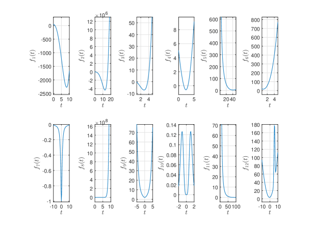
Figure 2: The plots of the test functions

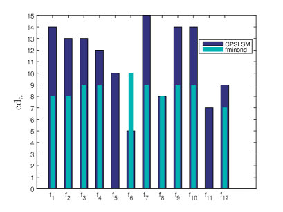
Figure 3: The cd_n for the CPSLSM and the fminbnd solver

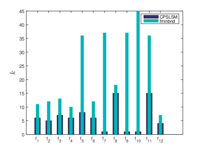
Figure 4: The number of iterations required by the CPSLSM and the fminbnd solver

Figures 5 and 6 show the cd_n and the number of iterations required by the CPSLSM using only first-order information versus the fminbnd solver. Here we notice that the obtained cd_n values using the CPSLSM are almost identical with the values obtained using second-order information with a slight increase in the number of iterations required for some test functions as expected.

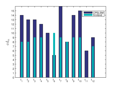
Figure 5: The cd_n for the CPSLSM using first-order information and the fminbnd solver

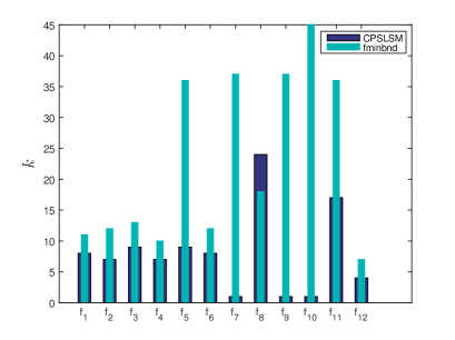
Figure 6: The number of iterations required by the CPSLSM using first-order information and the fminbnd solver

7.2 Multi-Dimensional Optimization Test Problems

The functions listed below are some of the common functions and data sets used for testing multi-dimensional unconstrained optimization algorithms:

• Sphere Function:

  $${f_{1}}(\bm{x})=\sum\limits_{i=1}^{d}{x_{i}^{2}},\quad d\in{\mathbb{Z}^{+}}.$$

  The global minimum function value is $f(\bm{x}^{*})=0$, obtained at $\bm{x}^{*}=[0,\ldots,0]^{T}$.

• Bohachevsky Function:

  $${f_{2}}(\bm{x})=x_{1}^{2}+2\,x_{2}^{2}-0.3\,\cos(3\,\pi{x_{1}})-0.4\,\cos(4\,\pi{x_{2}})+0.7.$$

  The global minimum function value is $f(\bm{x}^{*})=0$, obtained at $\bm{x}^{*}=[0,0]^{T}$.

• Booth Function:

  $${f_{3}}(\bm{x})={({x_{1}}+2\,{x_{2}}-7)^{2}}+{(2\,{x_{1}}+{x_{2}}-5)^{2}}.$$

  The global minimum function value is $f(\bm{x}^{*})=0$, obtained at $\bm{x}^{*}=[1,3]^{T}$.

• Three-Hump Camel Function:

  $${f_{4}}(\bm{x})=2\,x_{1}^{2}-1.05\,x_{1}^{4}+x_{1}^{6}/6+{x_{1}}\,{x_{2}}+x_{2}^{2}.$$

  The global minimum function value is $f(\bm{x}^{*})=0$, obtained at $\bm{x}^{*}=[0,0]^{T}$.

• Powell Function:

  $${f_{5}}(\bm{x})=\sum\limits_{i=1}^{d/4}{\left({{{({x_{4i-3}}+10\,{x_{4i-2}})}^{2}}+5\,{{({x_{4i-1}}-\,{x_{4i}})}^{2}}+{{({x_{4i-2}}-2\,{x_{4i-1}})}^{4}}+10\,{{({x_{4i-3}}-\,{x_{4i}})}^{4}}}\right)},\quad d\in{\mathbb{Z}^{+}}.$$

  The global minimum function value is $f(\bm{x}^{*})=0$, obtained at $\bm{x}^{*}=[0,\ldots,0]^{T}$.

• Goldstein-Price Function:

  $${f_{6}}(\bm{x}) =\left({1+{{({x_{1}}+{x_{2}}+1)}^{2}}\,\left(19-14\,{x_{1}}+3\,{x_{1}}^{2}-14\,{x_{2}}+6\,{x_{1}}\,{x_{2}}+3\,x_{2}^{2}\right)}\right)$$

  $$\times\left({30+{{(2\,{x_{1}}-3\,{x_{2}})}^{2}}\,\left(18-32\,{x_{1}}+12\,x_{1}^{2}+48\,{x_{2}}-36\,{x_{1}}\,{x_{2}}+27\,x_{2}^{2}\right)}\right).$$

  The global minimum function value is $f(\bm{x}^{*})=3$, obtained at $\bm{x}^{*}=[0,-1]^{T}$.

• Styblinski-Tang Function:

  $${f_{7}}(\bm{x})=\frac{1}{2}\sum\limits_{i=1}^{d}{\left({x_{i}^{4}-16\,x_{i}^{2}+5\,{x_{i}}}\right)},\quad d\in{\mathbb{Z}^{+}}.$$

  The global minimum function value is $f(\bm{x}^{*})=-39.16599\,d$, obtained at $\bm{x}^{*}=[-2.903534,\ldots,-2.903534]^{T}$.

• Easom Function:

  $${f_{8}}(\bm{x})=-\cos({x_{1}})\,\cos({x_{2}})\,{e^{-{{({x_{1}}-\pi)}^{2}}-{{({x_{2}}-\pi)}^{2}}}}.$$

  The global minimum function value is $f(\bm{x}^{*})=-1$, obtained at $\bm{x}^{*}=[\pi,\pi]^{T}$.

Table 2 shows a comparison between the modified BFGS method endowed with MATLAB “fminbnd” line search solver (MBFGSFMINBND) and the modified BFGS method integrated with the present CPSLSM (MBFGSCPSLSM) for the multi-dimensional test functions $f_{i},i=1,\ldots,8$. The modified BFGS method was performed using Algorithm 6 with $\mathbf{B}_{0}=\mathbf{I},k_{\max}=10^{4}$, and $p_{max}=10$. The gradients of the objective functions were approximated using central difference approximations with step-size $10^{-4}$. Both fminbnd method and CPSLSM were initiated using the uncertainty interval $[\hat{\varepsilon},10]$ with $\hat{\varepsilon}=3\,\varepsilon_{\text{mach}}$. The maximum number of iterations allowed for each line search method was $100$. Each line search method was considered successful at each iterate $k$ if the change in the approximate step length $\alpha_{k}$ is below $10^{-6}$. The CPSLSM was carried out using $m=6,\varepsilon_{c}=\varepsilon_{\text{mach}},\varepsilon_{D}=10^{-6}$, and ${{\mathcal{F}}}_{\max}=100$. Moreover, both MBFGSFMINBND and MBFGSCPSLSM were stopped whenever

$$\left\|{\nabla f\left({{\bm{x}^{(k)}}}\right)}\right\|_{2}<{10^{-12}},$$

or

$$\left\|{{\bm{x}^{(k+1)}}-{\bm{x}^{(k)}}}\right\|_{2}<{10^{-12}}.$$

Table 2 clearly manifests the power of the CPSLSM, where the running time and computational cost of the modified BFGS method can be significantly reduced.

Function	MBFGSFMINBND	MBFGSCPSLSM
$\bm{x}^{(0)}$	NI/fval/EN/ET	NI/fval/EN/ET
	$\bm{\tilde{x}}^{*}$	$\bm{\tilde{x}}^{*}$
$f_{1}(\bm{x})\;(d=4)$	$13/4.784e-31/6.917e-16/0.021$	$2/3.3895e-29/5.822e-15/0.011$
$[50,1,4,-100]^{T}$	$[-3.0928e-16,-6.186e-18,-2.4723e-17,6.1814e-16]^{T}$	$[2.6019e-15,5.2024e-17,2.0815e-16,-5.2038e-15]^{T}$
$f_{1}(\bm{x})\;(d=100)$	$13/3.8088e-31/6.172e-16/0.047$	$2/7.3153e-30/2.705e-15/0.013$
${[50,1,4,2.5,\ldots,2.5,-100]^{T}}$	Omitted	Omitted
$f_{2}(\bm{x})$	$412/0.88281/7.766e-01/0.592$	$16/0.46988/4.695e-01/0.078$
$[10,20]^{T}$	$[0.61861,-0.46953]^{T}$	$[6.001e-09,0.46953]^{T}$
$f_{3}(\bm{x})$	$1/6.3109e-30/1.884e-15/0.002$	$1/0/0/0.005$
$[2,2]^{T}$	$[0.\bar{9},3]^{T}$	$[1,3]^{T}$
$f_{4}(\bm{x})$	NI exceeded $10000$ (Failure)	$5/1.8396e-32/9.740e-17/0.021$
$[-0.5,1]^{T}$		$[-9.7238e-17,5.6191e-18]^{T}$
$f_{5}(\bm{x})\;(d=4)$	$29/5.4474e-23/2.732e-06/0.051$	$28/3.6165e-26/4.409e-07/0.141$
$[2,3,1,1]^{T}$	$[2.3123e-06,-2.3123e-07,1.0163e-06,1.0163e-06]^{T}$	$[3.7073e-07,-3.7073e-08,1.6667e-07,1.6667e-07]^{T}$
$f_{6}(\bm{x})$	NI exceeded $10000$ (Failure)	$53/3/9.577e-09/0.291$
$[-0.5,1]^{T}$		$[5.3617e-09,-1]^{T}$
$f_{7}(\bm{x})\;(d=4)$	$576/-128.39/\text{--}/1.125$	$11/-128.39/\text{--}/0.052$
$[-4,-4,5,5]^{T}$	$[-2.9035,-2.9035,2.7468,2.7468]^{T}$	$[-2.9035,-2.9035,2.7468,2.7468]^{T}$
$f_{7}(\bm{x})\;(d=12)$	$308/-342.76/\text{--}/0.680$	$35/-342.76/\text{--}/0.202$
${[3,-0.5,1.278,1,\ldots 1,0.111,4.5]^{T}}$	Omitted	Omitted
$f_{8}(\bm{x})$	NI exceeded $10000$ (Failure)	$3/-1/4.333e-14/0.037$
$[1,1]^{T}$		$[3.1416,3.1416]^{T}$

Table 2: A comparison between the BFGSFMINBND and the BFGSCPSLSM for the multi-dimensional test functions $f_{i},i=1,\ldots,8$. “NI” denotes the number of iterations required by the modified BFGS algorithm, “fval” denotes the approximate minimum function value, “EN” denotes the Euclidean norm of the error $\bm{x}^{*}-\bm{\tilde{x}}^{*}$, where $\bm{\tilde{x}}^{*}$ is the approximate optimal design vector, and “ET” denotes the elapsed time for implementing each method in seconds. The bar over $9$ is used to indicate that this digit repeats indefinitely

8 Conclusion

While there is a widespread belief in the optimization community that an exact line search method is unnecessary, as what we may need is a large step-size which can lead to a sufficient descent in the objective function, the current work largely adheres to the use of adaptive PS exact line searches based on Chebyshev polynomials. The presented CPSLSM is a novel exact line search method that enjoys many useful virtues: (i) The initial guesses of the solution in each new search interval are calculated accurately and efficiently using a high-order Chebyshev PS method. (ii) The function gradient values in each iteration are calculated accurately and efficiently using CPSDMs. On the other hand, typical line search methods in the literature endeavor to approximate such values using finite difference approximations that are highly dependent on the choice of the step-size – a usual step frequently shared by the optimization community. (iii) The method is adaptive in the sense of locating a search interval bracketing the solution when the latter does not lie within the starting uncertainty interval. (iv) It is able to determine highly accurate approximate solutions even when the starting uncertainty intervals are far away from the desired solution. (v) The accurate approximation to the objective function, quadratic convergence rate to the local minimum, and the relatively inexpensive computation of the derivatives of the function using CPSDMs are some of the many useful features possessed by the method. (vi) The CPSLSM can be efficiently integrated with the current state of the art multivariate optimization methods. In addition, the presented numerical comparisons with the popular rival Brent’s method verify further the effectiveness of the proposed CPSLSM. In general, the CPSLSM is a new competitive method that adds more power to the arsenal of line search methods by significantly reducing the running time and computational cost of multivariate optimization algorithms.

Appendix A Preliminaries

In this section, we present some useful results from approximation theory. The first kind Chebyshev polynomial (or simply the Chebyshev polynomial) of degree $n$, $T_{n}(x)$, is given by the explicit formula

$${T_{n}}(x)=\cos\left({n\,{{\cos}^{-1}}(x)}\right)\;\forall x\in[-1,1],$$ (A.1)

using trigonometric functions, or in the following explicit polynomial form [Snyder(1966)]:

$${T_{n}}(x)=\frac{1}{2}\sum\limits_{k=0}^{\left\lfloor{n/2}\right\rfloor}{T_{n-2k}^{k}\,{x^{n-2k}}},$$ (A.2)

where

$$T_{m}^{k}={2^{m}}{(-1)^{k}}\left\{{\frac{{m+2\,k}}{{m+k}}}\right\}\left(\begin{array}[]{c}m+k\\ k\end{array}\right),\quad m,k\geq 0.$$ (A.3)

The Chebyshev polynomials can be generated by the three-term recurrence relation

$$T_{n+1}(x)=2xT_{n}(x)-T_{n-1}(x),\quad n\geq 1,$$ (A.4)

starting with ${T_{0}}(x)=1$ and ${T_{1}}(x)=x$. They are orthogonal in the interval $[-1,1]$ with respect to the weight function $w(x)=\left(1-x^{2}\right)^{-1/2}$, and their orthogonality relation is given by

$$\left\langle{{T_{n}},{T_{m}}}\right\rangle_{w}=\int_{-1}^{1}{{T_{n}}(x)\,{T_{m}}(x)\,{{\left(1-{x^{2}}\right)}^{-\frac{1}{2}}}dx=\frac{\pi}{2}{c_{n}}{\delta_{nm}}},$$ (A.5)

where $c_{0}=2,c_{n}=1,n\geq 1$, and $\delta_{nm}$ is the Kronecker delta function defined by

$${\delta_{nm}}=\left\{{\begin{array}[]{*{20}{l}}{1,\quad n=m,}\\ {0,\quad n\neq m.}\end{array}}\right.$$

The roots (aka Chebyshev-Gauss points) of $T_{n}(x)$ are given by

$${x_{k}}=\cos\left({\frac{{2k-1}}{{2n}}\pi}\right),\quad k=1,\ldots,n,$$ (A.6)

and the extrema (aka CGL points) are defined by

$${x_{k}}=\cos\left({\frac{{k\pi}}{n}}\right),\quad k=0,1,\ldots,n.$$ (A.7)

The derivative of $T_{n}(x)$ can be obtained in terms of Chebyshev polynomials as follows [Mason and Handscomb (2003)]:

$$\frac{d}{{dx}}{T_{n}}(x)=\frac{n}{2}\frac{{{T_{n-1}}(x)-{T_{n+1}}(x)}}{{1-{x^{2}}}},\quad\left|x\right|\neq 1.$$ (A.8)

[Clenshaw and Curtis (1960)] showed that a continuous function $f(x)$ with bounded variation on $[-1,1]$ can be approximated by the truncated series

$$({P_{n}}f)(x)=\sum\limits_{k=0}^{n}{{}^{{}^{\prime\prime}}}{{a_{k}}\,{T_{k}}(x)},$$ (A.9)

where

$${a_{k}}=\frac{2}{n}\sum\limits_{j=0}^{n}{{}^{{}^{\prime\prime}}}{{f_{j}}\,{T_{k}}({x_{j}})},\quad n>0,$$ (A.10)

$x_{j},j=0,\ldots,n$, are the CGL points defined by Eq. (A.7), $f_{j}=f(x_{j})\,\forall j$, and the summation symbol with double primes denotes a sum with both the first and last terms halved. For a smooth function $f$, the Chebyshev series (A.9) exhibits exponential convergence faster than any finite power of $1/n$ [Gottlieb and Orszag (1977)].

Appendix B Pseudocodes of Developed Computational Algorithms

Algorithm 1 The CPSLSM Algorithm Using Second-Order Information

0:  Positive integer number $m$; twice-continuously differentiable nonlinear single-variable objective function $f$; maximum function value ${{\mathcal{F}}}_{\max}$; uncertainty interval endpoints $a,b$; relatively small positive numbers ${\varepsilon}_{c},\varepsilon_{D},\varepsilon$; maximum number of iterations $k_{\max}$.

0:  The local minimum $t^{*}\in[a,b]$.

  $\rho_{1}\leftarrow 1.618033988749895;\rho_{2}\leftarrow 2.618033988749895;e^{+}=a+b;e^{-}=b-a;k\leftarrow 0;x_{j}\leftarrow\cos\left(j\pi/4\right),\quad j=0,\ldots,4$.

  Calculate $c_{l}^{(k)},l=0,\ldots,\left\lfloor{k/2}\right\rfloor,k=0,\ldots,4$ using Eqs. (3.3); $\{\theta_{k},\tilde{c}_{k}\}_{k=0}^{4}$ using Eqs. (3.10) & (4.7), respectively.

  if $m\neq 4$ then

     $x_{D,j}\leftarrow\cos\left(j\pi/m\right),\quad j=0,\ldots,m$.

  else

     $x_{D,j}\leftarrow x_{j},\quad j=0,\ldots,4$.

  end if

  while $k\leq k_{\max}$ do

     flag $\leftarrow 0;\bm{{{\mathcal{F}}}_{x}}\leftarrow\left\{{f\left({\left({{e^{-}}{x_{j}}+{e^{+}}}\right)/2}\right)}\right\}_{j=0}^{4};{{\mathcal{F}}}_{x,\max}\leftarrow\|\bm{{{\mathcal{F}}}_{x}}\|_{\infty}$.

     if ${{\mathcal{F}}}_{x,\max}>{{\mathcal{F}}}_{\max}$ then

        $\bm{{{\mathcal{F}}}_{x}}\leftarrow\bm{{{\mathcal{F}}}_{x}}/{{\mathcal{F}}}_{x,\max}$.

     end if

     Calculate $\left\{{\tilde{f}}_{k},{\tilde{f}}_{k}^{(1)}\right\}_{k=0}^{4}$, using Eqs. (4) and Algorithm 2, and the coefficients $\{A_{j}\}_{j=1}^{2}$ using Eqs. (4.9a) & (4.9b), respectively.

     if $\left|A_{1}\right|<{\varepsilon}_{c}$ then

        Call Algorithm 3.

     else

        Calculate $\{A_{j}\}_{j=3}^{4}$ using Eqs. (4.9c) & (4.9d); $A_{\max}\leftarrow\mathop{\max}\limits_{1\leq j\leq 4}\left|{{A_{j}}}\right|$.

        if $A_{\max}>1$ then

           $A_{j}\leftarrow A_{j}/A_{\max},\quad j=1,\ldots,4$.

        end if

        Calculate the roots $\{\bar{x}_{i}\}_{i=1}^{3}$.

        if $\bar{x}_{i}$ is complex or $\left|\bar{x}_{i}\right|>1$ for any $i=1,2,3$ then

           $k\leftarrow k+1$; Call Algorithm 4; $e^{+}\leftarrow a+b;\tilde{x}_{1}\leftarrow(2\,\tilde{t}_{1}-e^{+})/e^{-}$; flag $\leftarrow 1$.

        else

           Determine ${\tilde{x}_{1}}$ using Eq. (4.18).

        end ifCompute $\bm{\mathcal{F^{\prime}}}$ and $\bm{\mathcal{F^{\prime\prime}}}$ at $\tilde{x}_{1}$.

        if $\bm{\mathcal{F^{\prime\prime}}}>\varepsilon_{\text{mach}}$ then

           Call Algorithm 5.

        end if

        if flag $=1$ then

           

           continue

        else

           Compute $\tilde{x}_{2}$ using Eq. (4.19).

           if $\tilde{x}_{1}>\tilde{x}_{2}$ then

              $a\leftarrow(e^{-}\tilde{x}_{2}+e^{+})/2$.

           else

              $b\leftarrow(e^{-}\tilde{x}_{2}+e^{+})/2$.

           end if

        end if$e^{+}\leftarrow a+b;e^{-}\leftarrow b-a;k\leftarrow k+1$.

     end if

  end while

  Output(‘Maximum number of iterations exceeded.’).

  return  $t^{*}$.

Algorithm 2 Calculating the Chebyshev Coefficients of the Derivative of a Polynomial Interpolant

0:  The Chebyshev coefficients $\{{{\tilde{f}}_{k}}\}_{k=0}^{4}$.

  $\tilde{f}_{4}^{(1)}\leftarrow 0$.

  $\tilde{f}_{3}^{(1)}\leftarrow 8\,\tilde{f}_{4}$.

  $\tilde{f}_{k}^{(1)}\leftarrow 2\,(k+1)\,\tilde{f}_{k+1}+\tilde{f}_{k+2}^{(1)},\quad k=2,1$.

  $\tilde{f}_{0}^{(1)}\leftarrow\tilde{f}_{1}+\tilde{f}_{2}^{(1)}/2$.

  return  $\{\tilde{f}_{k}^{(1)}\}_{k=0}^{4}$.

Algorithm 3 Linear/Quadratic Derivative Interpolant Case

0:  $m;f;a;b;e^{-};\rho_{1};\rho_{2};A_{2};k;k_{\max};\{x_{D,j}\}_{j=0}^{m};{{\mathcal{F}}}_{\max};\varepsilon_{c};\varepsilon_{D};\varepsilon$.

  if $\left|A_{2}\right|<\varepsilon_{c}$ then

     Calculate $\{A_{j}\}_{j=3}^{4}$ using Eqs. (4.9c) & (4.9d); $\bar{x}\leftarrow-A_{4}/A_{3}$.

     if $\left|\bar{x}\right|\leq 1$ then

        ${t^{*}}\leftarrow\frac{1}{2}\left({(b-a)\,\bar{x}+a+b}\right)$; Output($t^{*}$); Stop.

     end if

  end if

  $k\leftarrow k+1$; Call Algorithm 4;$e^{+}\leftarrow a+b;\tilde{x}_{1}\leftarrow(2\tilde{t}_{1}-e^{+})/e^{-};\bm{\mathcal{F}}\leftarrow\left\{{f\left({\left({{e^{-}}{x_{D,j}}+{e^{+}}}\right)/2}\right)}\right\}_{j=0}^{m}$; $\mathcal{F}_{1,\max}\leftarrow\|\bm{\mathcal{F}}\|_{\infty}$.

  if $\mathcal{F}_{1,\max}>{{\mathcal{F}}}_{\max}$ then

     $\bm{\mathcal{F}}\leftarrow\bm{\mathcal{F}}/\mathcal{F}_{1,\max}$.

  end ifCompute $\bm{\mathcal{F}^{\prime}}$ and $\bm{\mathcal{F}^{\prime\prime}}$ at $\tilde{x}_{1}$ using Eqs. (4.12)–(4.14).

  if $\bm{\mathcal{F}^{\prime\prime}}>0$ then

     Call Algorithm 5.

  end if

  continue

Algorithm 4 One-Step Golden Section Search Algorithm

0:  $f;a;b;e^{-};\rho_{1};\rho_{2};\varepsilon$.

  $t_{1}\leftarrow a+e^{-}/\rho_{2};t_{2}\leftarrow a+e^{-}/\rho_{1}$.

  if $f(t_{1})<f(t_{2})$ then

     $b\leftarrow t_{2};t_{2}\leftarrow t_{1};e^{-}\leftarrow b-a;t_{1}\leftarrow a+e^{-}/\rho_{2}$.

  else

     $a\leftarrow t_{1};t_{1}\leftarrow t_{2};e^{-}\leftarrow b-a;t_{2}\leftarrow a+e^{-}/\rho_{1}$.

  end if

  if $f(t_{1})<f(t_{2})$ then

     $\tilde{t}_{1}\leftarrow t_{1};b\leftarrow t_{2}.$

  else

     $\tilde{t}_{1}\leftarrow t_{2};a\leftarrow t_{1}.$

  end if

  $e^{-}\leftarrow b-a$.

  if $e^{-}\leq\varepsilon$ then

     $t^{*}\leftarrow\tilde{t}_{1}$; Output($t^{*}$); Stop.

  else

     return.

  end if

  return  $\tilde{t}_{1},a,b,e^{-}$.

Algorithm 5 The Chebyshev-Newton Algorithm

0:  $m;f;a;b;e^{-};e^{+};\tilde{x}_{1};k;k_{\max};\varepsilon_{D};\varepsilon;\bm{\mathcal{F}};\bm{\mathcal{F}^{\prime}};\bm{\mathcal{F}^{\prime\prime}}$.

  while $k\leq k_{\max}$ do

     Determine $\tilde{x}_{2}$ using Eq. (4.15); $k\leftarrow k+1$.

     if Condition (4.16) is satisfied then

        $t^{*}\leftarrow(e^{-}\tilde{x}_{2}+e^{+})/2$.

        Output($t^{*}$); Stop.

     else if $\left|{{{\tilde{x}}_{2}}}\right|>1$ then

        

        break

     else if $\left|\bm{\mathcal{F}^{\prime}}\right|<\varepsilon_{D}$ and $\left|\bm{\mathcal{F}^{\prime\prime}}\right|<\varepsilon_{D}$ then

        

        if $\tilde{x}_{2}>\tilde{x}_{1}$ then

           Apply Brent’s method on the interval $[(e^{-}{{\tilde{x}}_{1}}+e^{+})/2,{b}]$; Output($t^{*}$); Stop.

        else

           Apply Brent’s method on the interval $[a,(e^{-}{{\tilde{x}}_{1}}+e^{+})/2]$; Output($t^{*}$); Stop.

        end if

     else

        Calculate $\bm{\mathcal{F}^{\prime}}$ and $\bm{\mathcal{F}^{\prime\prime}}$ at $\tilde{x}_{2}$ using Eqs. (4.14); $\tilde{x}_{1}\leftarrow\tilde{x}_{2}$.

     end if

  end while

  return  $k,\tilde{x}_{1}$.

Algorithm 6 Modified BFGS Algorithm With a Line Search Strategy

0:  Objective function $f$; initial guess $\bm{x}^{(0)}$; an approximate Hessian matrix $\mathbf{B}_{0}$; maximum number of iterations $k_{\max}$; maximum direction size ${p_{{\max}}}$.

  $k\leftarrow 0$; calculate $\mathbf{B}_{k}^{-1}$, and the gradient vector $\nabla f\left({\bm{x}^{(k)}}\right)$.

  $\bm{x}^{*}\leftarrow{\bm{x}^{(k)}}$ if the convergence criterion is satisfied.

  ${\bm{p}_{k}}\leftarrow-\nabla f\left({\bm{x}^{(k)}}\right);{p_{{\text{norm}}}}\leftarrow{\left\|{{\bm{p}_{k}}}\right\|_{2}}.$

  if ${p_{{\text{norm}}}}>{p_{{\max}}}$ then

     ${\bm{p}_{k}}\leftarrow{\bm{p}_{k}}/{p_{{\text{norm}}}}.$ {Scaling}

  end if

  while $k\leq k_{\max}$ do

     Perform a line search to find an acceptable step-size $\alpha_{k}$ in the direction $\bm{p}_{k}$.

     $\bm{s}_{k}\leftarrow\alpha_{k}\bm{p}_{k}$.

     $\bm{x}^{(k+1)}\leftarrow\bm{x}^{(k)}+\alpha_{k}\bm{p}_{k}$. {Update the state vector}

     Calculate $\nabla f\left({\bm{x}^{(k+1)}}\right)$, and set $\bm{x}^{*}\leftarrow{\bm{x}^{(k+1)}}$ if the convergence criterion is satisfied.

     ${\bm{y}_{k}}\leftarrow\nabla f\left({\bm{x}^{(k+1)}}\right)-\nabla f\left({\bm{x}^{(k)}}\right);t\leftarrow\bm{s}_{k}^{T}{\bm{y}_{k}};\mathbf{T}_{1}\leftarrow{\bm{y}_{k}}\bm{s}_{k}^{T};\mathbf{T}_{2}\leftarrow{{\mathbf{B}}_{k}^{-1}}{\mathbf{T}_{1}}$.

     ${\mathbf{B}}_{k+1}^{-1}\leftarrow{\mathbf{B}}_{k}^{-1}+{\left({t+\bm{y}_{k}^{T}{{\mathbf{B}}_{k}^{-1}}{\bm{y}_{k}}}\right)\left({{\bm{s}_{k}}\bm{s}_{k}^{T}}\right)}/t^{2}-\left({\mathbf{T}_{2}+\mathbf{T}_{2}^{T}}\right)/{t}.$

     ${\bm{p}_{k+1}}\leftarrow-{\mathbf{B}}_{k+1}^{-1}\nabla f\left({{\bm{x}^{(k+1)}}}\right);{p_{{\text{norm}}}}\leftarrow{\left\|{{\bm{p}_{k+1}}}\right\|_{2}}.$

     if ${p_{{\text{norm}}}}>{p_{{\max}}}$ then

        ${\bm{p}_{k+1}}\leftarrow{\bm{p}_{k+1}}/{p_{{\text{norm}}}}.$ {Scaling}

     end if

     $k\leftarrow k+1$.

  end while

  Output(‘Maximum number of iterations exceeded.’).

  return  $\bm{x}^{*};f\left(\bm{x}^{*}\right)$.

References

- [Baltensperger (2000)] Baltensperger R (2000) Improving the accuracy of the matrix differentiation method for arbitrary collocation points. Applied Numerical Mathematics 33(1):143–149.
- [Baltensperger and Trummer (2003)] Baltensperger R, Trummer MR (2003) Spectral differencing with a twist. SIAM Journal on Scientific Computing 24(5):1465–1487.
- [Canuto et al (1988)] Canuto C, Hussaini MY, Quarteroni A, Zang TA (1988) Spectral Methods in Fluid Dynamics. Springer series in computational physics, Springer-Verlag.
- [Chong and Zak (2013)] Chong EK, Zak SH (2013) An Introduction to Optimization, vol 76. John Wiley & Sons.