Direct determinations of the nucleon and pion $\sigma$ terms at nearly physical quark masses

Abstract

We present a high statistics study of the pion and nucleon light and strange quark sigma terms using $N_{f}=2$ dynamical non-perturbatively improved clover fermions with a range of pion masses down to $m_{\pi}\sim 150$ MeV and several volumes, $Lm_{\pi}=3.4$ up to $6.7$, and lattice spacings, $a=0.06-0.08$ fm, enabling a study of finite volume and discretisation effects for $m_{\pi}\gtrsim 260$ MeV. Systematics are found to be reasonably under control. For the nucleon we obtain $\sigma_{\pi N}=35(6)$ MeV and $\sigma_{s}=35(12)$ MeV, or equivalently in terms of the quark fractions, $f_{T_{u}}=0.021(4)$, $f_{T_{d}}=0.016(4)$ and $f_{T_{s}}=0.037(13)$, where the errors include estimates of both the systematic and statistical uncertainties. These values, together with perturbative matching in the heavy quark limit, lead to $f_{T_{c}}=0.075(4)$, $f_{T_{b}}=0.072(2)$ and $f_{T_{t}}=0.070(1)$. In addition, through the use of the (inverse) Feynman-Hellmann theorem our results for $\sigma_{\pi N}$ are shown to be consistent with the nucleon masses determined in the analysis. For the pion we implement a method which greatly reduces excited state contamination to the scalar matrix elements from states travelling across the temporal boundary. This enables us to demonstrate the Gell-Mann-Oakes-Renner expectation $\sigma_{\pi}=m_{\pi}/2$ over our range of pion masses.

I Introduction

How the quark and gluon constituents of matter account for the properties of hadronic bound states is of fundamental interest. The decomposition for one of the most basic properties, the hadron mass, has been understood for some time Shifman et al. (1978); Ji (1995a, b), however, the magnitude of each contribution is as yet only approximately known due to its non-perturbative nature. Of particular importance are quark scalar matrix elements that form the quark contribution to the hadron mass. For the case of the nucleon, these matrix elements are also needed for determining the size of dark matter-nucleon scattering cross-sections for direct detection experiments (see, for example, Refs. Cline et al. (2013); Hietanen et al. (2014); Hill and Solon (2015a, b); Ellis et al. (2016); Abdallah et al. (2015)). A variety of approaches have been used to determine the scalar matrix elements or sigma terms from pion-nucleon scattering data Gasser et al. (1991); Pavan et al. (2002); Alarcón et al. (2013); Hoferichter et al. (2015a, 2016). Lattice calculations, as a first principles approach, are now gaining prominence, not least due to the refinement of techniques and increase in computational power available which now allows for the direct evaluation of the sigma terms at the physical point Yang et al. (2015a); Abdel-Rehim et al. (2016). In this work, we present results for the pion and nucleon scalar matrix elements close to the physical point, but also investigate the quark mass dependence up to $m_{\pi}\lesssim 500$ MeV and the lattice systematics including lattice spacing and volume dependence. On a technical note, our analysis includes a method for reducing excited state contamination to pion three-point functions by isolating the forward propagating pion for lattices with anti-periodic fermionic boundary conditions in time.

By way of introduction, we review the decomposition of hadron masses into the quark and gluon contributions and the scalar matrix elements of interest. The starting point is the energy momentum tensor of QCD Freedman et al. (1974); Freedman and Weinberg (1974); Caracciolo et al. (1990)

$$T_{\mu\nu}=\frac{1}{4}\sum_{q}\bar{q}\gamma_{(\mu}\overleftrightarrow{D}_{\nu)}q+F_{\mu\alpha}F_{\nu\alpha}-\frac{1}{4}\delta_{\mu\nu}F^{2}$$ (1)

and its anomalous trace Coleman and Jackiw (1971); Chanowitz and Ellis (1973); Crewther (1972); Nielsen (1977); Adler et al. (1977):

$$T_{\mu\mu}=(\gamma_{m}(\alpha)-1)\sum_{q}m_{q}\bar{q}q+\frac{\beta(\alpha)}{4\alpha}F^{2}.$$ (2)

For our conventions see Appendix A. We define the expectation value for the hadron state, $|H\rangle$:

$$\langle T_{\mu\nu}\rangle_{H} =\langle H|T_{\mu\nu}|H\rangle-\langle 0|T_{\mu\nu}|0\rangle$$

$$=\frac{\left\langle H|\int d^{3}x\,T_{\mu\nu}(x)|H\right\rangle}{\langle H|H\rangle}-\left\langle 0\left|\int\!d^{3}\!x\,T_{\mu\nu}(x)\right|0\right\rangle.$$ (3)

Since $-T_{44}$ is the Hamiltonian density, in the rest frame of the hadron $H$, $\langle T_{44}\rangle_{H}=-M_{H}$ gives the mass while $\langle T_{ij}\rangle_{H}=\langle T_{4i}\rangle_{H}=0$. This means that in any Lorentz frame:

$$m_{H} =-\langle T_{\mu\mu}\rangle_{H}$$

$$=\sum_{q}m_{q}\langle\bar{q}q\rangle_{H}-\gamma_{m}(\alpha)\sum_{q}m_{q}\langle\bar{q}q\rangle_{H}-\frac{\beta(\alpha)}{4\alpha}\langle F^{2}\rangle_{H}.$$ (4)

For zero momentum this is the same as Ji (1995a),

$$m_{H}=-\langle T_{44}\rangle_{H}=\underbrace{\sum_{q}m_{q}\langle\bar{q}q\rangle_{H}}_{\langle H_{m}\rangle_{H}}\underbrace{+\frac{1}{2}\langle\mathbf{B}^{2}-\mathbf{E}^{2}\rangle_{H}+\sum_{q}\langle\bar{q}{\bf D}\cdot\boldsymbol{\gamma}q\rangle_{H}}_{\langle H_{\rm kin}\rangle_{H}=3\langle H_{a}\rangle_{H}}\underbrace{-\frac{1}{4}\left[\gamma_{m}\sum_{q}m_{q}\langle\bar{q}q\rangle_{H}+\frac{\beta}{4\alpha}\langle\mathbf{E}^{2}+\mathbf{B}^{2}\rangle_{H}\right]}_{\langle H_{a}\rangle_{H}=\frac{1}{4}\left(m_{H}-\langle H_{m}\rangle_{H}\right)}.$$ (5)

The terms are grouped into scale invariant combinations Tarrach (1982): $\langle H_{m}\rangle_{H}$, the quark mass contribution, $\langle H_{\rm kin}\rangle_{H}$, arising from the quark and gluon kinetic energies and $\langle H_{a}\rangle_{H}$ from the trace anomaly. Comparison with Eq. (4) demonstrates that knowledge of the sigma terms $\sigma^{H}_{q}=m_{q}\langle\bar{q}q\rangle_{H}$ and $m_{H}$ is sufficient to determine all three components. We remark that the individual (scale dependent) quark and gluon kinetic energies can be computed on the lattice, however, this is not attempted here. In a theory with only two light quarks, $q=u,d$, then $\langle H_{m}\rangle_{N}=\sigma^{N}_{u}+\sigma^{N}_{d}=\sigma_{\pi N}$ for the nucleon. We define $\sigma^{\pi}_{u}+\sigma^{\pi}_{d}=\sigma_{\pi}$ for the light quark pion sigma term. Early estimates, employing Eq. (4) and SU(3) flavour symmetry breaking of baryon octet masses Cheng (1989) suggested $\sigma_{\pi N}\sim 26$ MeV, while $\sigma_{\pi}\sim m_{\pi}/2$ can be inferred from the Gell-Mann-Oakes-Renner (GMOR) relation and the Feynman-Hellmann theorem, $\sigma_{q}^{H}=m_{q}\partial m_{H}/\partial m_{q}$ (this was noted in Refs. Donoghue et al. (1990); Ananthanarayan et al. (2004); Yang et al. (2015b) and confirmed in Ref. Yang et al. (2015b) at $m_{\pi}=281$ MeV). Using $\sigma_{\pi N}\sim 35\,\mathrm{MeV}\,\sim 0.04\,m_{N}$, which is close to the result presented later in this paper, we have the decompositions for $N_{f}=2$ QCD:

$$m_{N} \approx\left(0.04\,m_{N}\right)_{m}+\left(0.72\,m_{N}\right)_{\rm kin}+\left(0.24\,m_{N}\right)_{\rm a},$$ (6)

$$m_{\pi} \approx\left(\frac{1}{2}m_{\pi}\right)_{m}+\left(\frac{3}{8}m_{\pi}\right)_{\rm kin}+\left(\frac{1}{8}m_{\pi}\right)_{\rm a},$$ (7)

reflecting the different impact of spontaneous chiral symmetry breaking in the two cases, i.e. $m_{N}>0$ for $m_{q}=0$. These decompositions will be modified in the presence of the sea quarks $s,c,b,t$. While the sigma terms for the light and strange quarks, $q=u,d,s$, must be determined via non-perturbative methods one can appeal to the heavy quark limit in order to evaluate $\sigma_{c,b,t}$. Following Ref. Shifman et al. (1978), in the effective theory the heavy quark ($h$) term $m_{h}\bar{h}h$, to leading order in the QCD coupling $\alpha$, transforms as $-(2/3)(\alpha/(8\pi))F^{2}+O\left(\Lambda^{2}/m_{h}^{2}\right)$, where $\Lambda$ is the typical QCD scale. One can then use Eq. (4) to express $\sigma_{h}$ in terms of the sum of the sigma terms for which $m_{q}\ll m_{h}$. To leading order in $1/m_{h}$ and $\alpha$ one obtains:

$$\sigma_{h=c,b,t}=\frac{2}{27}\left(m_{H}-\sum_{q=u,d,s}\sigma_{q}\right).$$ (8)

See Refs. Vecchi (2013); Hill and Solon (2015a) for radiative corrections. Alternatively, in terms of the quark mass fractions, $f_{T_{q}}=\sigma_{q}/m_{H}$,

$$m_{H}f_{T_{h}}=\frac{2}{27}m_{H}\left(1-\sum_{q=u,d,s}f_{T_{q}}\right)\equiv\frac{2}{27}m_{H}f_{T_{G}}.$$ (9)

For the nucleon, these quark fractions are needed to determine the coupling to the Standard Model Higgs boson or to other scalar particles, for example, in dark matter-nucleon scattering Cline et al. (2013); Hietanen et al. (2014); Hill and Solon (2015a, b); Ellis et al. (2016); Abdallah et al. (2015). The cross-section is proportional to $|f_{N}|^{2}$, where (using Eq. (9))

$$\frac{f_{\mathrm{N}}}{m_{\mathrm{N}}}\approx\sum_{q=u,d,s}f_{T_{q}}\frac{\alpha_{q}}{m_{q}}+\frac{2}{27}f_{T_{G}}\sum_{q=c,b,t}\!\!\frac{\alpha_{q}}{m_{q}}\,,$$ (10)

with the couplings $\alpha_{q}\propto m_{q}/m_{W}$ in the Higgs case.

For the light and strange sigma terms one can go further and disentangle the contributions from the valence and sea quarks through the ratios,

$$r^{\mathrm{sea}}=\frac{\langle\bar{u}u+\bar{d}d\rangle^{\mathrm{sea}}}{\langle\bar{u}u+\bar{d}d\rangle}\hskip 14.22636pt\mathrm{and}\hskip 14.22636pty =\frac{2\langle\bar{s}s\rangle}{\langle\bar{u}u+\bar{d}d\rangle},$$ (11)

while the SU(3) flavour symmetry of the sea is probed with the ratio

$$a^{\mathrm{sea}}=\frac{2\langle\bar{s}s\rangle}{\langle\bar{u}u+\bar{d}d\rangle^{\mathrm{sea}}}.$$ (12)

Other quantities of interest are the non-singlet sigma term, $\sigma_{0}=\frac{1}{2}(m_{u}+m_{d})\langle\bar{u}u+\bar{d}d-2\bar{s}s\rangle$ and the isospin asymmetry ratio

$$z=\frac{\langle\bar{u}u-\bar{s}s\rangle}{\langle\bar{d}d-\bar{s}s\rangle}.$$ (13)

In a naive picture of the proton with only valence quarks $z=1.5$. Using Gell-Mann-Okubo mass relations, Ref. Cheng (1989) estimated this to be only slightly modified to 1.49 in the presence of sea quarks. The individual light and strange quark sigma terms can be obtained from different combinations of $\sigma_{0}$, $z$ and $\sigma_{\pi N}$, see, for example, Ref. Cline et al. (2013).

Table 1: Details of the ensembles used in the analysis including the lattice spacing $a$, the light quark mass parameter $\kappa_{\ell}$, the lattice volume $V$, the pion mass $m_{\pi}$ and the spatial lattice extent $L$ in units of $m_{\pi}$. The finite volume pion masses were determined in Ref. Bali et al. (2014) and the errors include an estimate of both the systematic and statistical uncertainty. The number of configurations $n^{\rm conf}$ employed is given along with the number of measurements of the three-point functions on each configuration for the connected $n^{\rm 3pt,conn}_{N}$ and disconnected $n^{\rm 3pt,dis}_{N}$ contributions for the nucleon and similarly for the pion. The number of Wuppertal smearing iterations $n_{\mathrm{sm}}$ applied to the light quark appearing in the pion and nucleon interpolators is also shown.

Ensemble	$\beta$	$a$ [fm]	$\kappa_{\ell}$	$V$	$m_{\pi}$ [GeV]	$Lm_{\pi}$	$n^{\rm conf}$	$n^{\rm 3pt,conn}_{N}$	$n^{\rm 3pt,dis}_{N}$	$n^{\rm 3pt,conn}_{\pi}$	$n^{\rm 3pt,dis}_{\pi}$	$n_{\mathrm{sm}}$
I	5.20	0.081	0.13596	$32^{3}\times 64$	0.2795(18)	3.69	$1986$	$4$	8			300
II	5.29	0.071	0.13620	$24^{3}\times 48$	0.4264(20)	3.71	$1999$	$2$	8			300
III			0.13620	$32^{3}\times 64$	0.4222(13)	4.90	$1998$	$2$	8	2	8	300
IV			0.13632	$32^{3}\times 64$	0.2946(14)	3.42	$2023$	$2$	8	2	8	400
V				$40^{3}\times 64$	0.2888(11)	4.19	$2025$	$2$	8	2	8	400
VI				$64^{3}\times 64$	0.2895(07)	6.71	$1232$	$2$	8			400
VIII			0.13640	$64^{3}\times 64$	0.1497(13)	3.47	$1593$	$3$	8	3	8	400
IX	5.40	0.060	0.13640	$32^{3}\times 64$	0.4897(17)	4.81	$1123$	$2$	8			400
X			0.13647	$32^{3}\times 64$	0.4262(20)	4.18	$1999$	$2$	8			450
XI			0.13660	$48^{3}\times 64$	0.2595(09)	3.82	$2177$	$2$	8			600

This paper is organized as follows: in the next section we provide details of the simulation including the lattice set-up and the construction of the connected and disconnected quark line diagrams needed for the computation of the pion and nucleon scalar matrix elements. These matrix elements typically suffer from significant excited state contamination. The fitting procedures employed to ensure the ground states are extracted reliably is discussed in Sections II.2 and II.3, for the pion and the nucleon, respectively. Some of the quantities given above require renormalization due to the explicit breaking of chiral symmetry for our lattice fermion action. The relevant renormalization factors are detailed in Section II.4. Our final results for the sigma terms, including mass and volume dependence are presented in Section III for the pion and, also including lattice spacing effects, for the nucleon in Section IV. For the latter a comparison is made with other recent lattice determinations by direct and indirect (via the Feynman-Hellmann theorem) methods and also other theoretical results in Section V. We conclude in Section VI. For the sake of brevity, our conventions for the definition of the energy-momentum tensor are collected in Appendix A. For the pion, in order to reduce excited state contamination, we construct the relevant two- and three-point functions from quark propagators with both periodic and anti-periodic boundary conditions in time. This approach is discussed in Appendix B. Finally, the finite volume chiral perturbation theory expressions we use when investigating finite size effects on the sigma terms and nucleon mass are given in Appendix C.

II Simulation details

II.1 Lattice set-up and methods

Figure 1: Overview of the ensembles listed in Table 1. Colours indicate the lattice spacings and symbols the lattice extents. This labelling will be used in the figures presented in Secs. III–V. Different volume ranges are indicated by the horizontal lines.

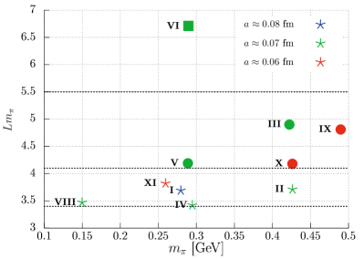
The analysis was performed on $N_{f}=2$ ensembles using the Wilson gauge action with non-perturbatively improved clover fermions generated by QCDSF and the Regensburg lattice QCD group (RQCD). A wide range of pion masses ($m_{\pi}=490$ MeV down to $150$ MeV) and spatial lattice extents ($Lm_{\pi}=3.4$ up to $6.7$) were realized over a limited range of lattice spacings ($a=0.08$ fm to $0.06$ fm). The scale was set using the value $r_{0}\approx 0.5$ fm at vanishing quark mass, obtained by extrapolating the nucleon mass to the physical point (within our range of $a$) Bali et al. (2013). Table 1 gives details of the ensembles and Fig. 1 illustrates the range of volumes available for each pion mass.

The full set of ensembles was used in the determination of the nucleon scalar matrix elements enabling a constrained approach to the physical point and a thorough investigation of finite volume effects using three spatial extents with $m_{\pi}\sim 290$ MeV at fixed lattice spacing. Discretisation effects are $\mathcal{O}(a^{2})$ for some non-singlet combinations of scalar currents and $\mathcal{O}(a)$ for others (see Section II.4). The latter being due to mixing with the gluonic operator $aF^{2}$ Bhattacharya et al. (2006) or $\mathcal{O}(am_{q})$ terms. Note that mixing with $aF^{2}$ is present also for other actions such as the twisted mass (including maximal twist) and overlap actions. No clear indication of significant discretisation effects is seen in our results, however, $a$ ($a^{2}$) only varies by a factor 1.3 (1.8) in our simulations and, hence, this cannot be checked decisively.

A further source of systematic uncertainty is excited state contamination. As in our studies of nucleon isovector quantities Bali et al. (2014, 2015) a careful investigation of excited state contributions is performed, see Sections II.2 and II.3 for the pion and nucleon, respectively. This is an important issue for our analysis of pion scalar matrix elements, since terms arising from multi-pion states which propagate around the temporal boundary can dominate the three-point function if the temporal extent of the lattice is not large. In particular, for the near physical point ensemble the temporal extent of the lattice is only $T\sim 4.58$ fm $\approx 3.5/m_{\pi}$. Our method for reducing this contribution and ensuring ground state dominance, detailed in Appendix B, was applied to four ensembles (labelled III, IV, V and VIII in Table 1) at one lattice spacing $a=0.07$ fm. The pion mass is varied between $420$ MeV and $150$ MeV and a limited study of finite size effects is possible through the use of two volumes with $Lm_{\pi}=3.4$ and $4.2$ for $m_{\pi}=290$ MeV.

Figure 2: Quark line connected ($C^{\mathrm{conn}}_{{\rm 3pt}}(t_{\mathrm{f}},t,t_{\mathrm{i}})$, top) and disconnected ($C^{\mathrm{dis}}_{{\rm 3pt}}(t_{\mathrm{f}},t,t_{\mathrm{i}})$, bottom) three-point functions for the nucleon. The quark contractions give a relative minus sign between the diagrams. Note that for scalar matrix elements, the vacuum expectation value of the current insertion needs to be subtracted ($\bar{q}q\mapsto\bar{q}q-\langle\bar{q}q\rangle$), see Eqs. (3) and (15). The blue lines represent light quarks. The disconnected loop is evaluated for both light and strange quarks.

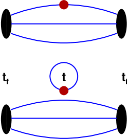
High statistics was achieved in all cases and the signals of the required two-point and three-point functions were further improved by performing multiple measurements per configuration using different source positions. This is necessary in particular for scalar matrix elements since the intrinsic gauge noise can be substantial. The isoscalar three-point functions contain both connected and disconnected quark line contributions, as shown in Fig. 2, with the latter dominating the noise. Eight measurements of the disconnected diagrams were performed on each configuration compared to two measurements for the connected part. Signal to noise ratios are worse for coarser lattice spacings and for smaller pion masses and the number of determinations of the connected terms was increased to $4$ and $3$ for ensembles I ($m_{\pi}=280$ MeV with $a\sim 0.08$ fm) and VIII ($150$ MeV, $a=0.07$ fm), respectively. For the nucleon the connected terms were generated as part of a previous study of isovector charges Bali et al. (2015). The number of disconnected measurements was not increased due to the computational cost and the limited reduction in error due to correlations within the data. Measurements performed on the same configuration are averaged and binning over configurations was applied to a level consistent with four times the integrated autocorrelation time.

Table 2: Results for the hadron masses and axial Ward identity masses ($\tilde{m}$) in lattice units, the source-sink separation for the connected three-point functions, $t_{\rm f}^{\rm conn}$ ($t^{\rm conn}_{\rm i}=0$), and the minimum source-operator insertion separation for the disconnected three-point function, $\Delta t_{\rm min}$. For the nucleon, the statistical errors of $C^{\mathrm{conn}}_{{\rm 3pt}}$ decrease for smaller values of $t_{\rm f}$, such that for ensembles IV and VIII it is sufficient to perform a smaller number of measurements per configuration (shown in brackets) than indicated in Table 1. In all cases the errors include both statistical and systematic uncertainties. For the axial Ward identity masses the asterisk (^∗) indicates which values are used to determine the ratio of non-singlet to singlet renormalization factors presented in Section II.4.

Ensemble	$am_{\pi}$	$am_{N}$	$a\tilde{m}$	$(t_{\mathrm{f}}/a)^{\rm conn}_{\rm nuc}$	$(t_{\mathrm{f}}/a)^{\rm conn}_{\rm pion}$	$\Delta t_{\mathrm{min}}/a$
I	0.11516(73)	0.4480(31)	0.003676(39)	13		4
II	0.15449(74)	0.4641(53)	0.007987(44)	15		4
III	0.15298(46)	0.4486(30)	0.007964(34)∗	15,17	32	5
IV	0.10675(51)	0.3855(46)	0.003794(28)	7(1),9(1),11(1),	32	4
				13,15,17
V	0.10465(38)	0.3881(35)	0.003734(21)	15	32	4
VI	0.10487(24)	0.3856(19)	0.003749(18)∗	15		5
VIII	0.05425(49)	0.3398(63)	0.000985(19)∗	9(1),12(2),15	32	5
IX	0.15020(53)	0.3962(34)	0.009323(25)∗	17		4
X	0.13073(61)	0.3836(32)	0.007005(23)∗	17		6
XI	0.07959(27)	0.3070(50)	0.002633(14)∗	17		5

In the two flavour theory the strange quark is quenched and the size of the corresponding systematic uncertainty is difficult to quantify (note that the dominant strange quark contribution can still be computed, c.f., for example, Eq. (11)). This source of uncertainty will be removed in future work on $N_{f}=2+1$ configurations generated as part of the CLS effort Bruno et al. (2015a). We fix the valence strange quark mass parameter, $\kappa_{s}$, by tuning the hypothetical strange-antistrange pseudoscalar meson mass to the value $(m_{K^{\pm}}^{2}+m_{K^{0}}^{2}-m_{\pi^{\pm}}^{2})^{1/2}\approx 686.9$ MeV within statistical errors, where experimental values are used for the kaon and pion masses.

The two-point and three-point functions, needed to extract the scalar matrix elements, have the form

$$C_{{\rm 2pt}}(t_{\mathrm{f}},t_{\mathrm{i}}) = \sum_{\vec{x}}\langle{\cal H}(\vec{x},t_{\mathrm{f}})\overline{{\cal H}}(\vec{0},t_{\mathrm{i}})\rangle,$$ (14)

$$C_{{\rm 3pt}}(t_{\mathrm{f}},t,t_{\mathrm{i}}) = \sum_{\vec{x},\vec{y}}\langle{\cal H}(\vec{x},t_{\mathrm{f}})S(\vec{y},t)\overline{{\cal H}}(\vec{0},t_{\mathrm{i}})\rangle$$ (15)

$$-\sum_{\vec{x},\vec{y}}\langle S(\vec{y},t)\rangle\langle{\cal H}(\vec{x},t_{\mathrm{f}})\overline{{\cal H}}(\vec{0},t_{i})\rangle,$$

for a hadron, ${\cal H}$, at rest created at a time $t_{\mathrm{i}}$, destroyed at a time $t_{\mathrm{f}}$ and with the operator $S=\bar{q}q$ inserted at a time $t$. The interpolators ${\cal H}=(u^{T}C\gamma_{5}d)u$ and $\bar{u}\gamma_{5}d$ for the proton and pion, respectively, create both ground and excited states with contributions which fall off exponentially with the energy of the state in Euclidean time. To improve the overlap with the ground state, spatially extended interpolators were constructed using Wuppertal smeared Güsken et al. (1989); Güsken (1990) light quarks with spatially APE smoothed gauge transporters Falcioni et al. (1985). The number of Wuppertal smearing iterations applied, $n_{\rm sm}$, shown in Table 1, was optimized for each ensemble such that ground state dominance was achieved at similar physical times for different light quark masses and lattice spacings, see Ref. Bali et al. (2015) for more details.

Wick contractions for the three-point function lead to the connected $C^{\mathrm{conn}}_{{\rm 3pt}}(t_{\mathrm{f}},t,t_{\mathrm{i}})$ and disconnected contributions $C^{\mathrm{dis}}_{{\rm 3pt}}(t_{\mathrm{f}},t,t_{\mathrm{i}})$, shown in Fig. 2 for the nucleon. The standard sequential source method is employed to determine the connected diagram. This provides the three-point function at all $t\in[t_{\mathrm{i}}+2a,t_{\mathrm{f}}-2a]$ for fixed $t_{\mathrm{f}}$, where the minimal distance $2a$ from source and sink is due to the use of clover fermions. Table 2 details the values of $t_{\mathrm{f}}$ chosen (relative to a source at the origin, i.e. $t_{\mathrm{i}}=0$). For the nucleon the relative statistical errors of $C^{\mathrm{conn}}_{{\rm 3pt}}$ increase rapidly with increasing $t_{\mathrm{f}}-t_{\mathrm{i}}$, motivating small source-sink separations. However, several $t_{\mathrm{f}}$ values are needed to check for excited state contributions which, as we will see in Sections II.2 and II.3, are significant for scalar matrix elements, even with optimized spatially extended interpolators. In the pion case, the signal does not decay rapidly with $t_{\mathrm{f}}$ and we choose $t_{\mathrm{f}}=T/2$. This has the advantage that $C_{{\rm 3pt}}(t_{\mathrm{f}},t,t_{\mathrm{i}})$ can be averaged over the regions with $t_{\mathrm{i}}=0<t<t_{\mathrm{f}}$ and $t_{\mathrm{f}}<t<t_{\mathrm{i}}=T$. Excited state contributions are controlled using our method discussed in Appendix B.

Figure 3: The time positions $t$ of the 8 disconnected loops and the source positions $t_{\mathrm{i}}$ of the 4 two-point functions which are used to construct the disconnected three-point function in Eq. (16), for an ensemble with $T=64a$ and minimum $|t-t_{\mathrm{i}}|=4a$.

Figure 4: (Left) A comparison of the effective masses of the pseudoscalar $C_{\rm 2pt}$ and $C_{\rm 2pt}^{\rm improv}$ for ensembles V (top) and VIII (bottom) with pion masses $m_{\pi}\sim 289$ MeV and $\sim 150$ MeV, respectively. The correlators are smeared at both the source and the sink (SS). Note that for $C_{\rm 2pt}$ the inverse cosh effective mass is shown. (Right) $C_{\rm 2pt}^{\rm improv}$ divided by the corresponding forward propagating ground state contribution, $A_{1}e^{-m_{\pi}t_{\rm f}}$ ($A_{1}=|Z_{01}|^{2}$), extracted from a fit, for the same ensembles.

The disconnected term is constructed from a disconnected “loop” $L(t)$ and a two-point function computed on each configuration:

$$C^{\mathrm{dis}}_{{\rm 3pt}}(t_{\mathrm{f}},t,t_{\mathrm{i}})=\langle C^{c}_{{\rm 2pt}}(t_{\rm f},t_{\mathrm{i}})L^{c}(t)\rangle_{c}-\langle C^{c}_{{\rm 2pt}}(t_{\rm f},t_{\mathrm{i}})\rangle_{c}\langle L^{c}(t)\rangle_{c},$$ (16)

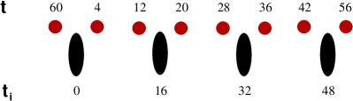
where $L^{c}(t)=\sum_{\vec{x}}\mathrm{Tr}[M^{-1}(x,x)\mathds{1}]$ on configuration $c$, $\langle\cdot\rangle_{c}$ makes the configuration average explicit and $x=(\vec{x},t)$. The quark propagator $M^{-1}(x,x)$ is estimated stochastically using 25 complex $\mathds{Z}_{2}$ random source vectors that are non-zero on 8 timeslices. This number of stochastic estimates and level of time partitioning for $L(t)$ ensured the additional random noise introduced to $C^{\mathrm{dis}}_{{\rm 3pt}}$ was below the level of the intrinsic gauge noise while also allowing for 8 measurements of the three-point function per configuration. The latter requires four different source times $t^{n}_{\mathrm{i}}=nT/4$, $n=0,1,2,3$ for the two-point functions appearing in Eq. (16). The disconnected loops are positioned at timeslices $t^{n}_{\mathrm{i}}\pm\Delta t_{\mathrm{min}}$, where $\Delta t_{\mathrm{min}}$ is a fixed minimum value of $|t-t_{\mathrm{i}}|$ for each ensemble, see Table 2. Figure 3 illustrates the relative positions of the disconnected loops and two-point function source times for the example of an ensemble with $T=64a$ and $\Delta t_{\mathrm{min}}=4a$. By correlating a forward (backward) propagating two-point function with source position $t^{n}_{\mathrm{i}}$ with a loop at $t_{\rm i}^{n}+\Delta t$ ($t_{\rm i}^{n}-\Delta t$), for each $n$ one obtains the 8 estimates of the disconnected three-point function,

$$C^{\mathrm{dis}}_{{\rm 3pt}}(\Delta t_{\mathrm{f}},\Delta t)\equiv \frac{1}{8}\sum_{n=0}^{3}\left\{\left[\langle C^{c}_{{\rm 2pt}}(t_{i}^{n}+\Delta t_{\rm f},t^{n}_{\mathrm{i}})L^{c}(t^{n}_{\mathrm{i}}+\Delta t)\rangle_{c}-\langle C^{c}_{{\rm 2pt}}(t_{i}^{n}+\Delta t_{\rm f},t^{n}_{\mathrm{i}})\rangle_{c}\langle L^{c}(t^{n}_{\mathrm{i}}+\Delta t)\rangle_{c}\right]_{t_{\mathrm{f}}>t>t_{\mathrm{i}}}\right.$$

$$\left.+\left[\langle C^{c}_{{\rm 2pt}}(t_{i}^{n}-\Delta t_{\rm f},t^{n}_{\mathrm{i}})L^{c}(t^{n}_{\mathrm{i}}-\Delta t)\rangle_{c}-\langle C^{c}_{{\rm 2pt}}(t_{i}^{n}-\Delta t_{\rm f},t^{n}_{\mathrm{i}})\rangle_{c}\langle L^{c}(t^{n}_{\mathrm{i}}-\Delta t)\rangle_{c}\right]_{t_{\mathrm{i}}>t>t_{\mathrm{f}}}\right\},$$ (17)

for multiple time separations $\Delta t=|t-t_{\rm i}|=\Delta t_{\mathrm{min}},T/4-\Delta t_{\mathrm{min}},T/4+\Delta t_{\mathrm{min}},\ldots<|t_{\mathrm{f}}-t_{\rm i}|\equiv\Delta t_{\mathrm{f}}$. In order to determine both the light and the strange quark content of the nucleon and pion, the loop $L^{c}(t)$ is evaluated both for $\kappa_{\ell}$ and $\kappa_{s}$ and contracted with the two-point function constructed from light quark propagators. For the nucleon, as we will see in Section II.3, the statistical noise increases rapidly with increasing source-operator insertion separations and only $\Delta t=\Delta t_{\mathrm{min}}$ and $\Delta t=T/4-\Delta t_{\mathrm{min}}$ provide useful signals. For the pion, several $\Delta t$ give meaningful results.

The connected and disconnected three-point functions are analysed separately to extract the corresponding contributions to the scalar matrix elements, $g_{S}^{\rm latt,conn}=\langle H|\bar{q}q|H\rangle^{\rm latt}_{\rm conn}$ and $g_{S}^{\rm latt,dis}=\langle H|\bar{q}q|H\rangle^{\rm latt}_{\rm dis}-\langle 0|\bar{q}q|0\rangle^{\rm latt}_{\rm dis}$, respectively, where $|H\rangle\propto\overline{{\cal H}}|0\rangle$ is a nucleon or pion state and we used the normalization $\langle H|H\rangle=1$, see below. This procedure is described in the next two sections.

II.2 Pion three-point function fits

Figure 5: The ratio of the pion connected three-point to two-point functions for both the standard ($R^{\rm conn}$) and improved ($R^{\rm improv,conn}$, Eq. (20)) cases, for ensembles III, IV, V and VIII. The blue and green shaded regions show the results for $g_{S}^{\rm latt,conn}$ obtained from a constant fit to $R^{\rm improv,conn}$ and a simultaneous fit to $C_{\rm 3pt}^{\rm improv,conn}$ and $C_{\rm 2pt}^{\rm improv}$ using Eqs. (21) and (22), respectively. The corresponding fits to Eq. (22) divided by the ground state two-point contribution, i.e. $B_{1}+B_{2}\left(e^{(t_{\rm f}-t)\Delta E}+e^{-t\Delta E}\right)$, are shown as the black lines. For ensemble III, a similar fit to the unimproved $C_{\rm 3pt}^{\rm conn}$ and $C_{\rm 2pt}$ is indicated by the dashed line and the resulting value of $g_{S}^{\rm latt,conn}$ as the pink region. In all cases the fitting range is indicated by the width of the shaded region and the range shown for the black and dashed lines. The fits shown are representative and, as discussed in the text, for the final results the variation arising from different fitting ranges is taken into account.

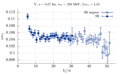
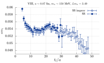
Pion three-point functions calculated on ensembles with anti-periodic boundary conditions in time can suffer from large contributions involving a backward propagating pion (across the boundary) in combination with a forward propagating scalar state, if the temporal extent of the lattice is not large and the pion mass is close to the physical value, as is the case, for example, for ensemble VIII (see Table 1). These contributions and our method for reducing them are discussed in detail in Appendix B. We utilize correlation functions computed using quark propagators with different temporal boundary conditions (periodic and anti-periodic) to isolate the forward propagating negative parity terms. This is illustrated in Fig. 4 for the two-point function on two representative ensembles with $m_{\pi}=289$ MeV and $150$ MeV.

Figure 6: (Top) The ratio $R^{\rm dis}(t_{\rm f},t,0)=C_{\rm 3pt}^{\rm dis}(t_{\rm f},t,0)/C_{\rm 2pt}(t_{\rm f},0)$ for the pion and $S=\bar{s}s$ with different values of the current insertion time $t$ on two ensembles with (left) $m_{\pi}=422$ MeV and (right) $m_{\pi}=150$ MeV. The correlation functions are smeared at both the source and the sink. The expectation value of the disconnected loop $\langle 0|S|0\rangle$ has been subtracted. (Bottom) The same ratios evaluated using improved correlation functions.

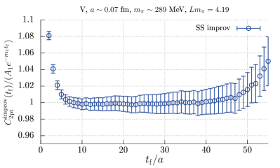
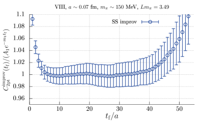
The expected time dependence of the “improved” two-point function, smeared at the source and sink (SS), is given by Eq. (69),

$$C^{\rm improv}_{{\rm 2pt}}(t_{\mathrm{f}},0)= |Z_{01}|^{2}e^{-t_{\rm f}E_{1}}\left[\vphantom{\frac{|Z_{12}|^{2}}{|Z_{01}|^{2}}}1+\frac{|Z_{12}|^{2}}{|Z_{01}|^{2}}e^{-(T-t_{\rm f})E_{2}}\right.$$

$$\left.+\frac{|Z_{03}|^{2}}{|Z_{01}|^{2}}e^{-t_{\rm f}(E_{3}-E_{1})}+\ldots\right],$$ (18)

where $t_{\rm i}=0$, $Z_{nm}=Z_{mn}^{*}=\langle n|{\cal\overline{H}}|m\rangle$. For simplicity we use the normalization convention $\langle m|n\rangle=\delta_{m,n}$, rather than the customary convention, $\langle 0|0\rangle=1$ and $\langle n|n\rangle=2E_{n}$. Note that $E_{1}=m_{\pi}$. The “$\ldots$” indicate the neglected higher excitations. We label the negative parity states by odd numbers where $E_{1}$ and $E_{3}$ are the masses of the ground state pion and a “three-pion” (or excited pion) state, respectively. The latter association is made since in nature the excited state pion is much heavier in mass. Similarly, the positive parity states are represented by even numbers and $E_{2}$ is the mass of a (scalar) “two-pion” state.

Figure 4 demonstrates that the contributions from the three-pion state (and higher negative parity states) die off rapidly due to the optimized smearing and that ground state dominance sets in around $t_{\rm f}=10a\approx 0.7$ fm for both ensembles, independent of the pion mass, and continues until $t_{\rm f}\sim 40a\approx 2.8$ fm. As one would expect, up to $t_{\rm f}=T/2$ there is no significant difference between the effective masses for the improved and unimproved two-point functions. The terms arising from scalar states propagating across the boundary become visible in the improved case for large $t_{\rm f}$ values. This can be seen in the combination $C^{\rm improv}_{{\rm 2pt}}(t_{\mathrm{f}},0)$, divided by the ground state contribution, $|Z_{01}|^{2}e^{-m_{\pi}t_{\rm f}}$, as determined from a fit, shown on the right in Fig. 4. For $t_{\rm f}/a\gtrsim 40$ this ratio (equal to the expression within the square brackets in Eq. (18)) increases from 1, with the deviation becoming more significant for smaller $m_{\pi}$. This motivates us to restrict $t_{\rm f}/a\leq 40$ in order to avoid similar terms when fitting to the pion three-point functions.

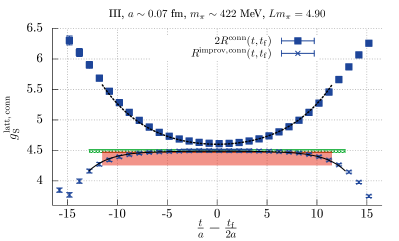
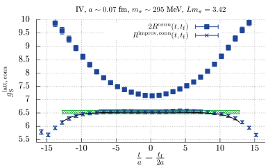
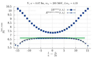
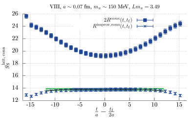
The connected three-point function is shown in Fig. 5 as a ratio with the two-point function for the four ensembles used in the pion analysis, with $m_{\pi}=422$ MeV down to $150$ MeV. In the mass-degenerate $N_{f}=2$ theory $\langle 1|\bar{u}u|1\rangle^{\rm conn}=\langle 1|\bar{d}d|1\rangle^{\rm conn}$ and only a single three-point function needs to be considered. Smeared sources and sinks are implemented and the sink time $t_{\rm f}$ is fixed to $T/2$. Using standard correlation functions, the ratio has the functional form, $0\leq t\leq t_{\rm f}$,

$$R^{\rm conn}(t_{\mathrm{f}},t,0)=\frac{C_{\rm 3pt}^{\rm conn}(t_{\rm f},t,0)}{C_{\rm 2pt}(t_{\rm f},0)} =\left[\langle 1|S|1\rangle^{\rm conn}+\frac{|Z_{12}|^{2}}{|Z_{01}|^{2}}\left(\langle 1|S|1\rangle^{\rm conn}e^{-(T-t_{\rm f})E_{2}}+\langle 2|S|2\rangle^{\rm conn}e^{-(T-2t_{\rm f})m_{\pi}}e^{-t_{\rm f}E_{2}}\right)\right.$$

$$\left.+\frac{Z^{*}_{01}Z_{21}}{|Z_{01}|^{2}}\langle 0|S|2\rangle^{\rm conn}e^{-(T-2t_{\rm f})m_{\pi}}\left(e^{-tE_{2}}+e^{-(t_{\rm f}-t)E_{2}}\right)\right]$$

$$\left[1+e^{-(T-2t_{\rm f})m_{\pi}}+\frac{|Z_{12}|^{2}}{|Z_{01}|^{2}}\left(e^{-(T-t_{\rm f})E_{2}}+e^{-t_{\rm f}E_{2}}e^{-(T-2t_{\rm f})m_{\pi}}\right)\right]^{-1},$$ (19)

up to terms involving a three-pion state.

Figure 7: Examples of fits performed to $R^{\rm improv,dis}(t_{\rm f},t,0)$ for the pion with a light quark loop on ensemble V ($m_{\pi}=289$ MeV). The black lines indicate the fit and the blue shaded region the value of $g_{S}^{\rm latt,dis}$ extracted in each case. The range shown for the black lines indicates the fit range. (Top) a simultaneous fit to the SS and SL ratios for multiple operator insertion times $t$, employing the parametrization given in Eq. (73). (Middle) a similar fit to SS ratios, (bottom) a constant fit to SS ratios.

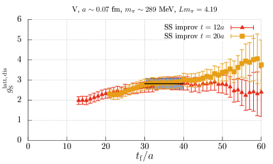
Employing our improved correlation functions, contributions arising from the backward propagating pion (those involving factors of $e^{-(T-2t_{\rm f})m_{\pi}}=1$ for $t_{\rm f}=T/2$) are removed and

$$R^{\rm improv,conn}(t_{\mathrm{f}},t,0) =\langle 1|S|1\rangle^{\rm conn}.$$ (20)

The considerable size of these contributions can be seen by comparing the improved and unimproved ratios, as shown in Fig. 5. The difference between the two cases becomes even more dramatic as $m_{\pi}$ decreases from $422$ MeV down to $150$ MeV. For $R^{\rm improv,conn}$ one can extract $\langle 1|S|1\rangle^{\rm conn}$ by fitting to a constant ($B_{1}$) for small $|t_{\rm f}/2-t|$. Examples of such fits are indicated by the blue regions in Fig. 5. However, the fitting range can be extended by including the next order terms arising from a forward propagating three-pion state. Equivalently, we perform simultaneous fits to $C_{\rm 3pt}^{\rm improv,conn}$ and $C_{\rm 2pt}^{\rm improv}$ using the functional form (see Eqs. (70) and (72) in Appendix B):

$$C_{\rm 2pt}^{\rm improv}(t_{\rm f},0) =A_{1}e^{-m_{\pi}t_{\rm f}}\left[1+A_{2}e^{-\Delta Et_{\rm f}}\right],$$ (21)

$$C_{\rm 3pt}^{\rm improv,conn}(t_{\rm f},t,0) =$$

$$A_{1}e^{-m_{\pi}t_{\rm f}}\left[B_{1}+B_{2}\left(e^{-(t_{\rm f}-t)\Delta E}+e^{-t\Delta E}\right)\right],$$ (22)

where $\Delta E=E_{3}-m_{\pi}$ and $B_{1}\sim\langle 1|S|1\rangle^{\rm conn}$. For both these fits and the constant fits to $R^{\rm improv,conn}$ we have to assume that contributions to $B_{1}$ containing factors $e^{-t_{\rm f}\Delta E}$ and $e^{-(T-t_{\rm f})E_{2}}$ are small for $t_{\rm f}=T/2$. If $E_{n}=nm_{\pi}$ then $e^{-t_{\rm f}\Delta E}=e^{-(T-t_{\rm f})E_{2}}\sim 0.03$ for the lightest pion mass ensemble, suggesting this assumption is reasonable. However, data with different $t_{\rm f}$ would be needed to confirm this.

Final values for $\langle 1|S|1\rangle^{\rm conn}$ are obtained taking into account the variation in the results due to the type of fit used and the fitting range chosen. For the latter all ranges with correlated $\chi^{2}/d.o.f.<2$ are included. If the covariance matrix for the fit is ill determined due to insufficient statistics the fit result can be biased. To avoid this problem the values for the scalar matrix elements are extracted for the different fitting ranges using uncorrelated fits.

We remark that for the $m_{\pi}=422$ MeV ensemble fitting to the unimproved $C_{\rm 3pt}^{\rm conn}$ and $C_{\rm 2pt}$ leads to a value for $\langle 1|S|1\rangle^{\rm conn}$ consistent with the improved result, albeit with larger statistical errors, see Fig. 5. The terms appearing in the numerator of Eq. (19) will dominate and one can see that $C_{\rm 3pt}^{\rm conn}$ will have the same $t$ dependence as in Eq. (22), replacing $\Delta E$ by $E_{2}$ (for fixed $t_{\rm f}=T/2$). If we assume that these effects only depend on $Tm_{\pi}$, which is approximately $9.8$ for this ensemble, then $T\lesssim 180a\sim 12.8$ fm would be required at $m_{\pi}=150$ MeV in order to ensure $\langle 1|S|1\rangle^{\rm conn}$ can be reliably extracted using standard correlators at $t_{\rm f}=T/2$. Having three-point functions with multiple $t_{\rm f}$ can help, however, at least one $t_{\rm f}$ value must be large enough that the unwanted terms are significantly suppressed.

Figure 8: Examples of simultaneous fits to proton SS $C_{{\rm 2pt}}(t_{\mathrm{f}},0)$ and the two SS connected $C_{{\rm 3pt}}^{{\rm conn}}(t_{\mathrm{f}},t)$ corresponding to $S=\bar{u}u$ and $\bar{d}d$, including multiple $t_{\rm f}$ values on ensembles IV and VIII ($m_{\pi}=295$ and $150$ MeV, respectively). The fit form is given in Eqs. (24) and (25). The data points are obtained by dividing the three-point function by the ground state contribution, $A_{1}e^{-m_{1}t_{\rm f}}$, where $A_{1}=|Z_{01}|^{2}$, as determined from the fit. The black lines indicate the fits while the green (blue) shaded region gives the resulting value for $\langle N_{1}|\bar{u}u|N_{1}\rangle^{\rm conn}$ ($\langle N_{1}|\bar{d}d|N_{1}\rangle^{\rm conn}$) and the width shows the fitting range chosen. For clarity the data points for $t_{\rm f}=12a$ on ensemble VIII are shown with open symbols.

Figure 9: A comparison of the results for the scalar matrix elements obtained from fits with multiple $t_{\rm f}$, as shown in Fig. 8, and fits to a single $t_{\rm f}=15a$ with the same fit range.

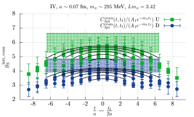
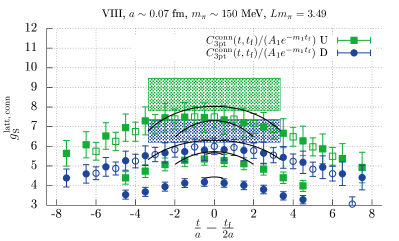
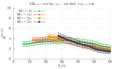
For the analysis of the disconnected contribution the three-point function has been computed for both $S=\bar{u}u$ ($\bar{d}d$) and $\bar{s}s$ at multiple current insertion times and for all sink times. In Fig. 6 we again consider the ratio with the two-point function for the improved and unimproved cases with a strange quark loop for ensembles III and VIII ($m_{\pi}=422$ MeV and $150$ MeV, respectively). Note that the correlators are smeared at the source and the sink. Including only the vacuum and pion state in the spectral decompositions of the correlators, the unimproved ratio has the time dependence,

$$R^{\rm dis}(t_{\rm f},t,0) =\frac{C_{\rm 3pt}^{\rm dis}(t_{\rm f},t,0)}{C_{\rm 2pt}(t_{\rm f},0)}$$

$$=\left(\langle 1|S|1\rangle^{\rm dis}-\langle 0|S|0\rangle^{\rm dis}\right)\frac{1}{1+e^{-m_{\pi}(T-2t_{\rm f})}},$$ (23)

independent of $t$. From Eq. (23), for small $t_{\rm f}>t$, one expects $R^{\rm dis}\sim\langle 1|S|1\rangle^{\rm dis}-\langle 0|S|0\rangle^{\rm dis}$. As $t_{\rm f}$ increases the ratio should drop to half of its value at $t_{\rm f}=T/2$ and continue to tend to zero, if contributions from states $|2\rangle,|3\rangle,\ldots$ are small. This behaviour is seen in Fig. 6 (top left) for the $m_{\pi}=422$ MeV ensemble in the limit of large $t<t_{\rm f}\leq T/2$. However, when the pion mass is decreased the terms arising from the backward propagating pion across the boundary (with forward propagating scalar $|2\rangle$), given in Eqs. (59) and (60), become very large and $R^{\rm dis}$ does not drop off significantly, as shown in Fig. 6 (top right) for $m_{\pi}=150$ MeV. Applying our improvement procedure, these terms are removed and one expects simply $R^{\rm improv,dis}(t_{\rm f},t,0)=\langle 1|S|1\rangle^{\rm dis}-\langle 0|S|0\rangle^{\rm dis}$ for $t_{\rm f}\ll T$. As observed in Fig. 6 (bottom), the improved ratio is constant for different current insertion times up to $t_{\rm f}\sim 40a$ on both ensembles. For larger $t_{\rm f}$ values, terms involving a backward propagating scalar particle cannot be ignored anymore.

In order to extract $\langle 1|S|1\rangle^{\rm dis}-\langle 0|S|0\rangle^{\rm dis}$ we perform three types of fits to $R^{\rm improv,dis}$: for SS correlators we fit the ratio to a constant and, whenever the next order terms can be resolved, also to a functional form which includes a three-pion state (Eq. (73)). The latter is also employed to fit the ratio constructed from correlators smeared at the source and local at the sink (SL), together with the SS ratio. As for the analysis of the connected part, the fitting range is varied with the restriction that the correlated $\chi^{2}/d.o.f.<2$, the final error taking into account the spread of results from uncorrelated fits due to different fit types and ranges. Representative examples of fits are given in Fig. 7 for a disconnected three-point function with a light quark loop on ensemble V ($m_{\pi}=289$ MeV).

II.3 Nucleon three-point function fits

For the nucleon scalar matrix elements three-point functions have been computed on all ensembles shown in Table 1. Note that we are working in the isospin limit but take the nucleon corresponding to a proton ($uud$). This distinction is only necessary for the connected part. For the latter excited state contamination is explored using multiple sink times at three pion masses, $m_{\pi}=426$ MeV, $289$ MeV and $150$ MeV, at the lattice spacing $a\approx 0.071$ fm. The standard fit form for SS correlators including contributions from the first excited state is derived from the spectral decomposition:

$$\,\,\,\,\,C_{{\rm 2pt}}(t_{\mathrm{f}})=|Z_{01}|^{2}e^{-m_{1}t_{\mathrm{f}}}\left[1+\frac{|Z_{02}|^{2}}{|Z_{01}|^{2}}e^{-\Delta mt_{\mathrm{f}}}+\ldots\right],$$ (24)

$$C_{{\rm 3pt}}(t_{\mathrm{f}},t)=|Z_{01}|^{2}e^{-m_{1}t_{\mathrm{f}}}\left[\vphantom{\frac{|Z_{12}|^{2}}{|Z_{01}|^{2}}}\langle N_{1}|S|N_{1}\rangle\right.$$

$$\left.\,\,\,\,\,\,+\frac{Z_{20}^{*}Z_{10}}{|Z_{01}|^{2}}\langle N_{2}|S|N_{1}\rangle\left(e^{-\Delta m(t_{\mathrm{f}}-t)}+e^{-\Delta mt}\right)\right.$$

$$\left.\,\,\,\,\,\,+|Z_{02}|^{2}\langle N_{2}|S|N_{2}\rangle e^{-\Delta mt_{\mathrm{f}}}+\ldots\vphantom{\frac{1}{2}}\right],$$ (25)

where $Z_{i0}=\langle N_{i}|{\cal\overline{N}}|0\rangle$ are the overlaps of the state ${\cal\overline{N}}|0\rangle$, created by a nucleon interpolator ${\cal\overline{N}}$ with the ground and first excited nucleon states $|N_{1}\rangle$ and $|N_{2}\rangle$, respectively. We denote the corresponding masses as $m_{1}$ and $m_{2}$ and the mass difference as $\Delta m=m_{2}-m_{1}$. For the connected three-point function there are two contributions arising from the scalar current $S=\bar{u}u$, inserted on a $u$ quark line, and similarly for $S=\bar{d}d$, inserted on the $d$ quark line. Both contributions are fitted simultaneously along with the two-point function to extract $\langle N_{1}|\bar{u}u|N_{1}\rangle^{\rm conn}$ and $\langle N_{1}|\bar{d}d|N_{1}\rangle^{\rm conn}$, respectively. With data at several values of $t_{\rm f}$, see Table 2, the last term in Eq. (25) can be resolved as well as the dependence on the current insertion time $t$.

Figure 10: The ratio $R^{\rm dis}(t_{\rm f},t,0)$ for the nucleon with a light quark loop as a function of $t_{\rm f}$ and $t$ on ensembles IX, V and VIII ($m_{\pi}=490$ MeV, $289$ MeV and $150$ MeV, respectively). The green shaded regions indicate the value of $g_{S}^{\rm latt,dis}$ extracted in each case. For ensembles IX and V constant fits are performed to the ratios with $t=4a,12a$ simultaneously with fit ranges $t_{\rm f}/a=9-32,17-32$ and $7-30,15-30$, respectively, while for ensemble VIII a constant fit is performed to the ratio with $t=11a$ with fit range $t_{\rm f}/a=12-18$.

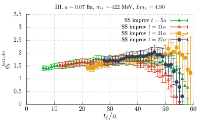
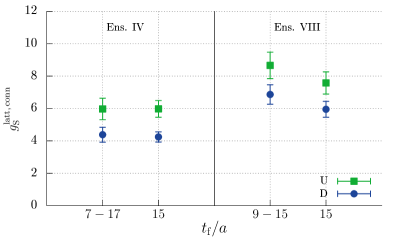
Typical simultaneous fits to two-point and multiple three-point functions (including different $t_{\rm f}$ values and both the $S=\bar{u}u$ and $\bar{d}d$ contributions) are illustrated in Fig. 8 for ensembles IV and VIII with $m_{\pi}=295$ MeV and $t_{\rm f}=7a,9a,11a,13a,15a,17a\sim 0.5-1.2$ fm and $m_{\pi}=150$ MeV and $t_{\rm f}=9a,12a,15a\sim 0.6-1.1$ fm, respectively. While contamination from excited states can certainly be resolved, the last term in Eq. (25) which only depends on the sink time does not appear to be significant for $t_{\rm f}\gtrsim 13a\sim 0.9$ fm. This can be seen in Fig. 8 from the consistency between the data with $t_{\rm f}=13a,15a,17a$ for $m_{\pi}=295$ MeV and $t_{\rm f}=13a,15a$ for $m_{\pi}=150$ MeV. Performing fits to a single $t_{\rm f}=15a\sim 1.1$ fm (in this case the last term cannot be distinguished from the first term in Eq. (25)), we find consistent results for the scalar matrix elements with the multi-$t_{\rm f}$ fit results, as demonstrated in Fig. 9. This gives us confidence that, for the interpolators employed, excited state contamination can be accounted for in the analysis of the other ensembles where three-point functions were generated with a single sink time $t_{\rm f}\gtrsim 1.0$ fm.

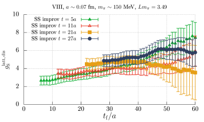
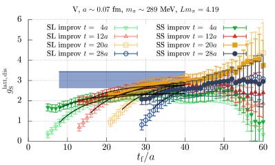
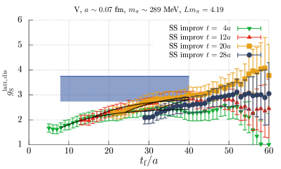
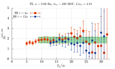
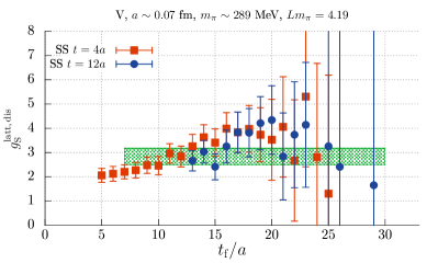
The disconnected scalar matrix element was extracted from the ratio of SS three-point and two-point functions. In contrast to the pion, the signal deteriorates fairly rapidly for $t_{\rm f}\sim 1.5$ fm, as seen in Fig. 10, and only the smallest two values of the current insertion time $t$ are useful, where $t_{\rm f}>t$. The figure also shows that excited state contributions are small on the scale of the statistical errors and indeed fits employing Eq. (73) failed to resolve such terms. The SL ratios were not included in the analysis as in this case the excited state contamination was too large to be modelled by including only the first excited state in the fit function. For most ensembles, constant fits were performed to the SS ratios for the two values of $t$ simultaneously. Statistical noise is larger for coarser lattice spacings and as the pion mass decreases. For ensemble I ($a\sim 0.08$ fm) only $t=4a\sim 0.32$ fm provided a reasonable signal, while for ensemble VIII, $m_{\pi}=150$ MeV, $t=5a$ and $11a$ are both noisy, however, we took the conservative choice to fit to $t=11a$.

In the same way as discussed for the analysis of the pion three-point functions in the previous section, the final results for both the connected and disconnected matrix elements include an estimate of the systematic uncertainty arising from the fitting procedure, obtained by varying the fitting range.

II.4 Renormalization

The renormalization of the lattice scalar matrix elements in the $N_{f}=2$ theory has already been discussed in detail in Ref. Bali et al. (2012) and we only repeat the relevant relations here. In the continuum the combination $m_{q}\langle H|\bar{q}q|H\rangle$ is invariant under renormalization group transformations. However, Wilson fermions explicitly break chiral symmetry and this enables mixing with other quark flavours. The renormalization factor that determines the strength of this mixing is $r_{m}=Z_{m}^{s}/Z_{m}^{ns}$, the ratio of the singlet ($Z_{m}^{s}$) to non-singlet ($Z_{m}^{ns}$) mass renormalization factors. This ratio can be determined non-perturbatively from the slope of the axial Ward identity quark mass ($\tilde{m}_{q}$) as a function of the vector Ward identity mass ($m_{q}$), see, e.g, Ref. Bhattacharya et al. (2006):

$$\tilde{m}_{q} =\frac{Z_{m}^{ns}Z_{P}^{ns}}{Z_{A}^{ns}}r_{m}m_{q}+O(am^{2}),\,$$ (26)

where the quark masses are defined as

$$m_{q} =\frac{1}{2a}\left(\frac{1}{\kappa_{q}}-\frac{1}{\kappa_{c,\rm sea}}\right)\hskip 2.84544pt\mathrm{and}\hskip 2.84544pt\tilde{m}_{q}=\frac{1}{2}\frac{\partial_{t}\langle A_{4}^{I}(t)P^{\dagger}(0)\rangle}{\langle P(t)P^{\dagger}(0)\rangle}.$$ (27)

$A_{4}^{I}$ and $P$ denote the $\mathcal{O}(a)$ improved axial-vector current and the pseudoscalar operator, respectively, with corresponding renormalization factors $Z_{A}^{ns}$ and $Z_{P}^{ns}$. $\kappa_{c,\rm sea}$ denotes the critical mass parameter along the isosymmetric line for which the quark mass is zero.

We employ the fit form

$$\tilde{m}_{q} =\frac{Zr_{m}}{2}\left(\frac{1}{\kappa_{q}}-\frac{1}{\kappa_{c,\rm sea}}\right)\left(1+\frac{b}{2}\left[\frac{1}{\kappa_{q}}-\frac{1}{\kappa_{c,\rm sea}}\right]\right),$$ (28)

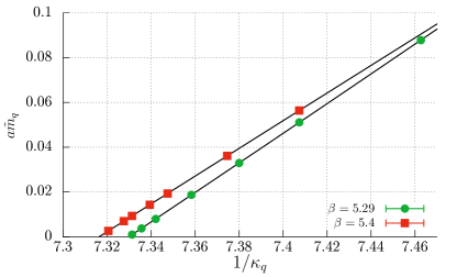
accounting for higher order contributions via a quadratic term. The coefficient $b$ is a combination of improvement coefficients which include, for instance, $b_{g}$ Bhattacharya et al. (2006), which is not known non-perturbatively. Values for $Z=Z_{m}^{ns}Z_{P}^{ns}/Z_{A}^{ns}$ are taken from Ref. Fritzsch et al. (2010), while $r_{m}$, $\kappa_{c,\rm sea}$ and $b$ are extracted from fits to a range of masses for $\beta=5.29$ and $\beta=5.40$: those indicated in Table 2 (chosen from ensembles with the largest $Lm_{\pi}$ for each $\kappa_{q}$) and at heavier quark masses produced by QCDSF and UKQCD Göckeler et al. (2006); Pleiter . For $\beta=5.20$ we use $r_{m}$ and $\kappa_{c,\rm sea}$ as determined in Ref. Fritzsch et al. (2012). Figure 11 shows examples of typical fits and Table 3 details the results, where the errors include systematics estimated by varying the fit range and including and omitting the quadratic term.

Figure 11: The axial Ward identity masses as functions of the inverse of the sea quark mass parameter $1/\kappa_{q}$ for $\beta=5.29$ ($a=0.07$ fm) and $\beta=5.40$ ($a=0.06$ fm). A typical fit is shown in each case obtained using Eq. (28).

Table 3: The critical hopping parameters $\kappa_{\mathrm{crit}}$ and ratio of singlet to non-singlet renormalization constants, $r_{m}$. The errors given include systematics. For $\beta=5.20$ the values quoted were determined by the ALPHA Collaboration Fritzsch et al. (2012).

$\beta$	$\kappa_{\mathrm{c,\rm sea}}$	$r_{m}$
5.20	0.1360546(39)	1.549(42)
5.29	0.1364281(12)	1.314(20)
5.40	0.1366793(11)	1.205(14)

The renormalization pattern for the scalar matrix elements is the same for the pion and the nucleon. We consider a general hadronic state $|H\rangle$, with the abbreviation:

$$\langle\bar{q}q\rangle^{\rm latt}= \langle H|\bar{q}q|H\rangle^{\rm latt}-\langle 0|\bar{q}q|0\rangle^{\rm latt}$$

$$= \langle H|\bar{q}q|H\rangle^{\rm latt,conn}+\langle H|\bar{q}q|H\rangle^{\rm latt,dis}$$

$$-\langle 0|\bar{q}q|0\rangle^{\rm latt}.$$ (29)

Note that for the strange quark, the connected term is not present. The dimension three scalar current ($\bar{q}q$ above refers to the current, integrated over space, and is dimensionless) will receive contributions $\propto a^{-3}\mathds{1}$, however, these cancel as we subtract the vacuum expectation value. Flavour singlet and non-singlet currents not only renormalize differently but are also subject to different $\mathcal{O}(a)$ improvement terms. In general, terms of the type $bam_{q}$ and $a\langle F^{2}\rangle$ can be added, where the second term can only affect flavour-singlet combinations. In the $N_{f}=2$ theory, the first type of term cancels from combinations like $(m_{u}+m_{d})\langle\bar{u}u+\bar{d}d\rangle$ Bhattacharya et al. (2006).

Following Ref. Bali et al. (2012), the light quark scalar matrix elements are given by

$$\sigma_{u} =\left[m_{u}\langle\bar{u}u\rangle\right]^{\mathrm{ren}}=\frac{1}{r_{m}}\left[m_{u}^{\mathrm{latt}}+\frac{(r_{m}-1)}{2}\left(m_{u}^{\mathrm{latt}}+m_{d}^{\mathrm{latt}}\right)\right]\left[\langle\bar{u}u\rangle^{\mathrm{latt}}+\frac{(r_{m}-1)}{2}\langle\bar{u}u-\bar{d}d\rangle^{\mathrm{latt}}\right],$$ (30)

$$\sigma_{d} =\left[m_{d}\langle\bar{d}d\rangle\right]^{\mathrm{ren}}=\frac{1}{r_{m}}\left[m_{d}^{\mathrm{latt}}+\frac{(r_{m}-1)}{2}\left(m_{u}^{\mathrm{latt}}+m_{d}^{\mathrm{latt}}\right)\right]\left[\langle\bar{d}d\rangle^{\mathrm{latt}}-\frac{(r_{m}-1)}{2}\langle\bar{u}u-\bar{d}d\rangle^{\mathrm{latt}}\right],$$ (31)

where $m_{q}^{\rm latt}$ is the $m_{q}$ of Eq. (27). Summing the two sigma terms in the isospin limit, the renormalization factors drop out,

$$\sigma_{u}+\sigma_{d} =\frac{m_{u}^{\mathrm{latt}}+m_{d}^{\mathrm{latt}}}{2}\langle\bar{u}u+\bar{d}d\rangle^{\mathrm{latt}},$$ (32)

as expected for the $N_{f}=2$ theory. Another combination of interest which does not require renormalization is the isospin asymmetry ratio,

$$z =\left[\frac{\langle\bar{u}u-\bar{s}s\rangle}{\langle\bar{d}d-\bar{s}s\rangle}\right]^{\mathrm{ren}}=\frac{\langle\bar{u}u-\bar{s}s\rangle^{\rm latt}}{\langle\bar{d}d-\bar{s}s\rangle^{\rm latt}}.$$ (33)

The non-singlet sigma term,

$$\sigma_{0} =\left[\frac{m_{u}+m_{d}}{2}\langle\bar{u}u+\bar{d}d-2\bar{s}s\rangle\right]^{\mathrm{ren}}$$

$$=r_{m}\frac{m_{u}^{\mathrm{latt}}+m_{d}^{\mathrm{latt}}}{2}\langle\bar{u}u+\bar{d}d-2\bar{s}s\rangle^{\mathrm{latt}}\,,$$ (34)

is only multiplicatively renormalized.

For the (quenched) strangeness matrix element we find

$$\sigma_{s} =\left[m_{s}\langle\bar{s}s\rangle\right]^{\mathrm{ren}}=\left[m_{s}^{\mathrm{latt}}+\frac{r_{m}-1}{2}\left(m_{u}^{\mathrm{latt}}+m_{d}^{\mathrm{latt}}\right)\right]\left(\langle\bar{s}s\rangle^{\mathrm{latt}}-\frac{(r_{m}-1)}{2r_{m}}\langle\bar{u}u+\bar{d}d\rangle^{\mathrm{latt}}\right)\,.$$ (35)

Large cancellations occur for this quantity at moderate lattice spacings ($a\gtrsim 0.06$ fm). This can only be mitigated by moving to finer lattices where $r_{m}$ is closer to $1$.

Finally, we give the expressions for the ratio of the sea to total light quark matrix elements,

$$r^{\mathrm{sea}} =\left[\frac{\langle\bar{u}u+\bar{d}d\rangle^{\mathrm{dis}}}{\langle\bar{u}u+\bar{d}d\rangle}\right]^{\mathrm{ren}}=r_{m}\left(\frac{\langle\bar{u}u+\bar{d}d\rangle^{\mathrm{latt,dis}}}{\langle\bar{u}u+\bar{d}d\rangle^{\mathrm{latt}}}-1\right)+1\,,$$ (36)

the ratio of the strange to (light) sea contributions,

$$a^{\mathrm{sea}} =\left[\frac{2\langle\bar{s}s\rangle}{\langle\bar{u}u+\bar{d}d\rangle^{\mathrm{dis}}}\right]^{\mathrm{ren}}=\frac{2r_{m}\langle\bar{s}s\rangle^{\mathrm{latt}}+(1-r_{m})\langle\bar{u}u+\bar{d}d\rangle^{\mathrm{latt}}}{r_{m}\langle\bar{u}u+\bar{d}d\rangle^{\mathrm{latt,dis}}+(1-r_{m})\langle\bar{u}u+\bar{d}d\rangle^{\mathrm{latt}}}\,,$$ (37)

and the ratio $y=a^{\mathrm{sea}}/r^{\mathrm{sea}}$,

$$y =\left[\frac{2\langle\bar{s}s\rangle}{\langle\bar{u}u+\bar{d}d\rangle}\right]^{\mathrm{ren}}=r_{m}\left(\frac{2\langle\bar{s}s\rangle^{\mathrm{latt}}}{\langle\bar{u}u+\bar{d}{d}\rangle^{\mathrm{latt}}}-1\right)+1\,.$$ (38)

Table 4: Final results for the pion sigma terms on a subset of ensembles at $\beta=5.29$ with $a=0.071$ fm. The errors given include both the systematic and statistical uncertainty, see the text. The finite volume corrected pion masses ($m_{\pi}^{\infty}$) were determined in Ref. Bali et al. (2015) using Ref. Colangelo et al. (2005), while $\sigma_{\pi}^{\infty}$ was obtained using the finite volume expressions for the pion mass Gasser and Leutwyler (1987, 1988) and the Feynman-Hellmann theorem, as detailed in Appendix C.

Ensemble	$Lm_{\pi}$	$m_{\pi}$ [GeV]	$m^{\infty}_{\pi}$ [GeV]	$m^{\infty}_{\pi}/2$ [GeV]	$\sigma_{\pi}$ [GeV]	$\sigma^{\infty}_{\pi}$ [GeV]	$\sigma_{s}$ [GeV]
III	4.90	0.4222(13)	0.4215(13)	0.2108(7)	0.2176(86)	0.2184(86)	0.014(11)
IV	3.42	0.2946(14)	0.2895(07)	0.1448(4)	0.1336(41)	0.1348(41)	-0.011(10)
V	4.19	0.2888(11)	0.2895(07)	0.1448(4)	0.1560(75)	0.1566(75)	0.031(20)
VIII	3.47	0.1497(13)	0.1495(13)	0.0748(7)	0.0780(42)	0.0782(42)	0.006(33)

Figure 12: Results for the finite volume pion light and strange quark sigma terms, $\sigma_{\pi}=\sigma_{u}+\sigma_{d}$ (top left) and $\sigma_{s}$ (top right), respectively, and the ratio of the sea to total light quark matrix elements, $r^{\mathrm{sea}}$ (bottom left), as a function of the pion mass. Both the statistical uncertainty (inner error bar) and the total systematic and statistical uncertainty (outer error bar) are shown. For $\sigma_{\pi}$, the results are compared to $m_{\pi}/2$ as determined in the simulation (indicated by a line, starting from zero which goes through the central values of $m_{\pi}/2$ for each ensemble). The symbols and colours for the data points correspond to those used in Fig. 1 for the different ensembles. The vertical lines indicate the physical point in the isospin limit, $m^{\rm phys}_{\pi}=135$ MeV. Also displayed (bottom right) is the infinite volume pion mass squared as a function of the renormalized quark mass obtained from the axial Ward identity, $m_{q}^{\overline{\rm MS}}(2\,\mathrm{GeV})=Z_{A}(1+am_{q}(b_{A}-b_{P}))\tilde{m}_{q}/Z_{P}^{\overline{\rm MS}}(2\,\mathrm{GeV})$ for all ensembles, see Table 2 for the values of $a\tilde{m}$ and Ref. Bali et al. (2015) for $b_{A}-b_{P}$, $Z_{A}$ and $Z_{P}^{\overline{\rm MS}}(2\,\mathrm{GeV})$. The shaded region shows a fit of the form $Cm_{q}^{\overline{\rm MS}}(2\,\mathrm{GeV})$ to all data points.

We remark that all the quantities in Eqs. (30) to (38) do not depend on a renormalization scale. Considering discretisation effects, only $z$ is automatically $\mathcal{O}(a)$ improved while all other observables are subject to $\mathcal{O}(a)$ lattice artifacts. However, not all $\mathcal{O}(a)$ terms are likely to be large, for example, the $a\langle F^{2}\rangle$ term does not contribute to $\sigma_{0}$ and if there is SU(3) flavour symmetry in the sea then for $a^{\rm sea}\approx 1$ it cancels.

III Pion sigma terms

Table 5: Final results for the pion-nucleon sigma term, $\sigma_{\pi N}$, the individual quark sigma terms of the proton, $\sigma_{q=u,d,s}$, the $y$ ratio and the isospin asymmetry ratio $z$. The errors include an estimate of both the systematic and statistical uncertainty, see the text. The values for the finite volume corrected pion mass, $m_{\pi}^{\infty}$, were determined as in Ref. Bali et al. (2015), using Ref. Colangelo et al. (2005). For $\sigma_{\pi N}^{\infty}$, we used Ref. Ali Khan et al. (2004), together with the Feynman-Hellmann theorem, as discussed in Appendix C.

Ensemble	$m_{\pi}$ [GeV]	$Lm_{\pi}$	$m^{\infty}_{\pi}$ [GeV]	$\sigma_{\pi N}$ [GeV]	$\sigma^{\infty}_{\pi N}$ [GeV]	$\sigma_{u}$ [GeV]	$\sigma_{d}$ [GeV]	$\sigma_{s}$ [GeV]	$y$	$z$
I	0.2795(18)	3.69	0.2783(18)	0.108(07)	0.115(07)	0.0614(36)	0.0462(33)	0.025(16)	0.070(046)	1.357(52)
II	0.4264(20)	3.71	0.4215(13)	0.191(14)	0.214(18)	0.1086(81)	0.0829(65)	0.030(12)	0.118(046)	1.361(60)
III	0.4222(13)	4.90	0.4215(13)	0.230(11)	0.238(12)	0.1299(64)	0.1000(55)	0.055(14)	0.178(039)	1.375(27)
IV	0.2946(14)	3.42	0.2895(07)	0.125(14)	0.135(15)	0.0709(81)	0.0542(61)	0.041(18)	0.108(050)	1.353(51)
V	0.2888(11)	4.19	0.2895(07)	0.132(10)	0.137(11)	0.0739(54)	0.0583(51)	0.048(23)	0.119(051)	1.312(31)
VI	0.2895(07)	6.71	0.2895(07)	0.108(11)	0.108(11)	0.0620(56)	0.0459(53)	-0.009(28)	-0.028(089)	1.338(29)
VIII	0.1497(13)	3.47	0.1495(13)	0.042(08)	0.043(08)	0.0232(42)	0.0182(35)	-0.036(64)	-0.068(132)	1.258(81)
IX	0.4897(17)	4.81	0.4883(17)	0.275(16)	0.288(17)	0.1605(83)	0.1148(81)	0.053(15)	0.192(046)	1.518(23)
X	0.4262(20)	4.18	0.4241(20)	0.226(15)	0.241(17)	0.1294(86)	0.0967(67)	0.062(15)	0.199(042)	1.442(39)
XI	0.2595(09)	3.82	0.2588(09)	0.107(07)	0.112(07)	0.0595(35)	0.0471(32)	0.075(18)	0.191(038)	1.335(35)

Our final results for the pion sigma terms for four ensembles at $a=0.071$ fm are presented in Table 4 and Fig. 12. The central values are obtained by taking the average of the maximum and minimum of the sigma terms that result from independently varying the fit ranges of the connected and disconnected contributions and, where relevant, the renormalization factor $r_{m}\pm\delta r_{m}$, where $\delta r_{m}$ is the error given in Table 3. The systematic error is then half of the difference of the maximum and minimum values. This is added in quadrature to the statistical error arising from typical fits to the connected and disconnected terms (computed by combining the jackknife samples of the individual contributions). For the pion sigma term in the infinite volume limit, $\sigma^{\infty}_{\pi}$, a further systematic arising from the finite volume correction is added in quadrature corresponding to half the size of the correction applied.

As discussed in Section I, we expect $\sigma_{\pi}=m_{\pi}/2$ for small pion masses. Fig. 12 shows this holds up to $m_{\pi}$ of at least $420$ MeV. The 2.62 $\sigma$ increase going from $Lm_{\pi}=3.42$ (ensemble IV) to $4.19$ (ensemble V) for $m_{\pi}\sim 290$ MeV suggests finite volume effects may be an issue. Chiral perturbation theory (ChPT) provides a framework for evaluating these effects, as detailed in Appendix C. The sigma term increases in the infinite volume limit, however, the corrections turn out to be very small, well below the level of statistical significance. The difference at $m_{\pi}\sim 290$ MeV is only reduced to 2.55$\sigma$ for $\sigma_{\pi}^{\infty}$, see Table 4. If the next-to-leading order (NLO) finite volume formula (Eq. (79)) is valid down to $Lm_{\pi}=3.4$ then the difference in the sigma terms can be ascribed to statistical variation. It is worth noting that without the use of our method for reducing excited state contamination to the pion scalar matrix element (see Section II.2 and Appendix B) the agreement with the GMOR expectation would not have been found. In particular, for the near physical point one may obtain $\sigma_{\pi}\sim 97$ MeV.

Figure 13: The pion-nucleon sigma term as a function of the pion mass. The symbols and colours of the data points correspond to those used in Fig. 1. Both the statistical uncertainty (inner error bar) and the total statistical and systematic uncertainty (outer error bar) are displayed. The vertical lines indicate the physical point in the isospin limit, $m^{\rm phys}_{\pi}=135$ MeV. (Left) Recent results from ETMC Dinter et al. (2012); Abdel-Rehim et al. (2016) and $\chi$QCD Yang et al. (2015a) vs. $m_{\pi}^{2}$ are compared to our finite volume values. Note that only the unitary values with purely statistical errors have been included from Ref. Yang et al. (2015a). (Right) The finite volume corrected results in the combination $(m^{\rm phys}_{\pi}/m_{\pi}^{\infty})^{2}\sigma^{\infty}_{\pi N}$ which has a linear dependence on $m_{\pi}^{\infty}$ at leading order (Eq. (41)). The blue shaded region indicates a fit of the form $a+bm_{\pi}^{\infty}$, with $\pm 1\sigma$ error band for $m_{\pi}\lesssim 420$ MeV. Similarly, the green shaded region shows a fit using $a+bm_{\pi}^{\infty}+c(m_{\pi}^{\infty})^{2}\ln(m^{\infty}_{\pi}/\lambda)$, where the linear coefficient is fixed using Eq. (41) and our determination of $g_{A}/F_{\pi}=13.88(29)$ GeV^-1 Bali et al. (2015) and $\lambda=1$ GeV.

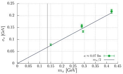
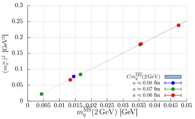
The observed behaviour of $\sigma_{\pi}$ suggests the GMOR relation is valid over the same range of pion masses. This is demonstrated in the bottom right panel of Fig. 12 where $({m_{\pi}^{\infty}})^{2}$ is shown as a function of the renormalized quark mass for all ensembles. A fit to the simple form $(m_{\pi}^{\infty})^{2}=Cm^{\overline{\rm MS}}_{q}(2\,\mathrm{GeV})$ for $m_{\pi}^{\infty}\lesssim 500$ MeV gives a $\chi^{2}/d.o.f.=1.9$ and a slope $C=-2\Sigma/F^{2}=5.04(1)(14)$ GeV, where $\Sigma$ is the chiral condensate and $F$ is the pion decay constant in the chiral limit. The second error is due to the uncertainty in the non-perturbative renormalization factors, given in Ref. Bali et al. (2015). Additional uncertainties, such as discretisation effects and, clearly, higher orders in the quark mass expansion have not been estimated (although given that $\chi^{2}/d.o.f.=1.9$, these terms appear to be small). This slope compares favourably with $2\Sigma/F^{2}=-5.3(5)$ obtained using FLAG estimates Aoki et al. (2014) $-\Sigma=(0.269(8)\,\mathrm{GeV})^{3}$ and $F_{\pi}/F=1.0744(67)$ for the $N_{f}=2$ theory with $F_{\pi}=92.2$ MeV.

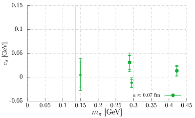
Recalling the decomposition of the mass of a hadron in Eq. (5), the $u$ and $d$ quark sigma term accounts for half the mass of the pion, i.e. approximately $68$ MeV at the physical point. From the ratio $r^{\rm sea}$ in Fig. 12, we find less than $15\%$ of this is due to (light) sea quarks. While the disconnected terms are significant, approximately $30\%$ in size of the connected terms, their contribution is reduced under renormalization (Eq. (36)) since $r_{m}=Z^{s}_{m}/Z^{ns}_{m}>1$. The strange quark contribution to the pion mass is likely to be small, however, again due to cancellations under renormalization, the overall uncertainties are large and we find $\sigma_{s}<50$ MeV. Within errors, $\sigma_{s}$ is also consistent with zero.

IV Nucleon $\sigma$ terms

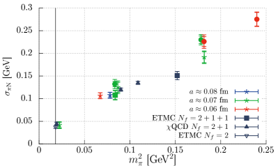
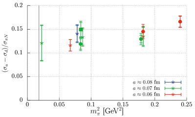
Starting with the pion-nucleon sigma term, our final results on all ensembles are given in Table 5 and displayed as a function of $m_{\pi}^{2}$ in Fig. 13 (left). The combined systematic and statistical errors are calculated as described in the previous section for the pion. The sigma term tends to zero as expected as the pion mass is reduced with no significant dependence on the lattice spacing, but some variation with the volume at heavier $m_{\pi}$. Reasonable agreement is seen with other recent direct determinations from ETMC Dinter et al. (2012); Abdel-Rehim et al. (2016) and $\chi$QCD Yang et al. (2015a), in particular, close to the physical point. These other (near) physical point simulations were performed at coarser lattice spacings, $a\sim 0.09$ fm and $0.11$ fm, respectively, and in the case of the ETMC on smaller volumes in terms of $Lm_{\pi}=2.97$ Abdel-Rehim et al. (2015) and, for the $\chi$QCD study, much lower statistics. We remark that $\mathcal{O}(a)$ discretisation errors arise for all fermion actions due to mixing with $aF^{2}$ and, so far, these effects have not been removed.

Table 6: Our determinations of the sigma terms, the ratios $y$ and $z$ and the quark mass fractions, $f_{T_{q=u,s,d,c,b,t}}$ for the proton, at the physical point. The errors encompass all systematics, see the text. Note that $\sigma_{\pi N}$, $\sigma_{0}$, $\sigma_{q=u,d}$, $(\sigma_{u}-\sigma_{d})/(\sigma_{u}+\sigma_{d})$, $f_{T_{q=u,d}}$ and $z$ are obtained using the $m_{\pi}=150$ MeV results, while $\sigma_{s}$, $f_{T_{s}}$ and $y$ are derived from fits in the range $m_{\pi}\lesssim 420$ MeV. Finite volume corrections have been applied to the light quark sigma terms, see the text. In order to extract $f_{T_{c,b,t}}$ we used $\sum_{q=u,d,s}f_{T_{q}}$ together with the perturbative relations in Refs. Chetyrkin et al. (1998); Hill and Solon (2015a), see the text.

$\sigma_{\pi N}$ (MeV)	$\sigma_{0}$ (MeV)	$\sigma_{u}$ (MeV)	$\sigma_{d}$ (MeV)	$\sigma_{s}$ (MeV)	$y$	$z$
35.0(6.1)	37.1(7.3)	19.6(3.4)	15.4(3.5)	34.7(12.2)	0.104(51)	1.258(81)
$\frac{\sigma_{u}-\sigma_{d}}{\sigma_{u}+\sigma_{d}}$	$f_{T_{u}}$	$f_{T_{d}}$	$f_{T_{s}}$	$f_{T_{c}}$	$f_{T_{b}}$	$f_{T_{t}}$
0.12(4)	0.021(4)	0.016(4)	0.037(13)	0.075(4)	0.072(2)	0.070(1)

The leading pion mass dependence of $\sigma_{\pi N}$ is provided by the application of the Feynman-Hellmann theorem to the NLO baryon ChPT expansion of the nucleon mass Steininger et al. (1998); Becher and Leutwyler (1999),

$$m_{N} =m_{N}^{0}-4c_{1}m_{\pi}^{2}-\frac{3(g^{0}_{A})^{2}m_{\pi}^{3}}{32\pi F^{2}}+O\left(m_{\pi}^{4}\ln\left(\frac{m_{\pi}}{\lambda}\right)\right),$$ (39)

which to this order contains the low energy constant, $c_{1}$, the renormalization scale $\lambda\sim m_{N}$ and the chiral limit nucleon mass, $m_{N}^{0}$, axial charge, $g^{0}_{A}\sim 1.22$ and pion decay constant, $F\sim 86$ MeV. At this order $g_{A}^{0}/F$ can be replaced by $g_{A}/F_{\pi}$. From $\sigma_{\pi N}=m_{\pi}^{2}\partial m_{N}/\partial m_{\pi}^{2}$ one finds,

$$\sigma_{\pi N} =m_{\pi}^{2}\left[-4c_{1}-\frac{9(g^{0}_{A})^{2}m_{\pi}}{64\pi F^{2}}+O\left(m_{\pi}^{2}\ln\left(\frac{m_{\pi}}{\lambda}\right)\right)\right].$$ (40)

We find it more meaningful to show in Fig. 13 (right) the combination

$$\frac{\sigma_{\pi N}}{m_{\pi}^{2}}(m_{\pi}^{\rm phys})^{2}=$$

$$(m_{\pi}^{\rm phys})^{2}\left[-4c_{1}-\frac{9(g^{0}_{A})^{2}m_{\pi}}{64\pi F^{2}}+O\left(m_{\pi}^{2}\ln\left(\frac{m_{\pi}}{\lambda}\right)\right)\right],$$ (41)

which has a milder dependence on the pion mass but also tends to the physical value as $m_{\pi}\to m_{\pi}^{\rm phys}$, where we take $m^{\rm phys}_{\pi}=135$ MeV in the electrically neutral isospin limit. The finite volume corrections to the sigma term can be derived in a similar way starting from the corresponding ChPT expressions for the nucleon mass, see Appendix C. The size of the corrections, as shown in Table 5, corresponds to 1–2 standard deviations for the larger pion mass ensembles ($m_{\pi}\gtrsim 420$ MeV), becoming much smaller as $m_{\pi}$ approaches the physical point. The shift is always to larger values of the sigma term for $L\to\infty$. The biggest effect is at $m_{\pi}\approx 420$ MeV between ensembles II ($Lm_{\pi}=3.71$) and III ($Lm_{\pi}=4.90$). The difference in $\sigma_{\pi N}$ for these two ensembles is $39(18)$ MeV, which is reduced to $24(22)$ MeV for the infinite volume value $\sigma^{\infty}_{\pi N}$. At $m_{\pi}\approx 290$ MeV the results from the smaller two ensembles, IV ($Lm_{\pi}=3.42$) and V ($Lm_{\pi}=4.19$) become slightly more coincident after finite volume corrections are applied, while between ensembles V and VI ($Lm_{\pi}=6.71$) this is less so. However, all differences are within the expected range for statistical variations.

Figure 14: The strange quark mass fraction $f_{T_{s}}$ (left) and $y$ ratio (right) as a function of $m_{\pi}^{2}$. Recent determinations by ETMC Dinter et al. (2012); Alexandrou et al. (2015a); Abdel-Rehim et al. (2016), Engelhardt Engelhardt (2012) and $\chi$QCD Yang et al. (2015a) (unitary values only) are also shown. The results are displayed as in Fig. 13. For both quantities, the blue (green) shaded regions indicate constant (constant plus linear in $m_{\pi}^{2}$) fits with $\pm 1\sigma$ error band for $m_{\pi}\lesssim 420$ MeV.

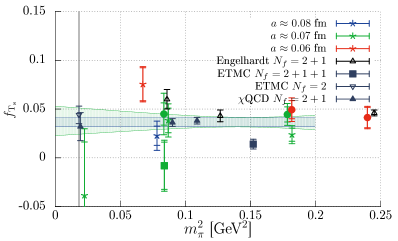
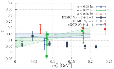
To test whether our statistically more precise results at $m_{\pi}\gtrsim 260$ MeV are consistent with the near physical point value, we perform a phenomenological fit to $\frac{\sigma^{\infty}_{\pi N}}{(m^{\infty}_{\pi})^{2}}(m_{\pi}^{\rm phys})^{2}$ based on Eq. (41) of the form (a) $a-bm_{\pi}^{\infty}$, with $a$ and $b$ determined from the fit and (b) $a-bm_{\pi}^{\infty}+c(m_{\pi}^{\infty})^{2}\ln(m^{\infty}_{\pi}/\lambda)$, setting $\lambda=1$ GeV and with $b$ fixed using $g_{A}/F_{\pi}=13.88(29)$ GeV^-1 Bali et al. (2015). The fit range is the same throughout, $m_{\pi}\lesssim 420$ MeV (including the $150$ MeV point), which gives us roughly three pion mass values, see Fig. 13 (right). Higher orders in the expansion are needed to include the $m_{\pi}\sim 500$ MeV data point. Figure 13 (right) shows both fits give consistent results at the physical point, only slightly below the central value for $m_{\pi}\sim 150$ MeV, with $a=0.037(3)$ GeV, $b=0.031(9)$ and $\chi^{2}/d.o.f.=1.0$ for fit (a) and $a=0.039(3)$ GeV, $c=-0.33(2)$ GeV^-1 and $\chi^{2}/d.o.f.=1.1$ for fit (b). The slope from fit (a) is significantly smaller than the ChPT expectation of $9g_{A}^{2}(m_{\pi}^{\rm phys})^{2}/(64\pi F_{\pi}^{2})\sim 0.16$. We comment more on the application of ChPT to $\sigma_{\pi N}$ and $m_{N}$ in Section V. The spread in the results at $m_{\pi}\sim 290$ MeV due to volume and lattice spacing dependence, and similarly at $m_{\pi}\sim 420$ MeV is less than the total uncertainty of the near physical point result. This observation, together with the insignificant remaining extrapolation, motivates us to quote $\frac{\sigma^{\infty}_{\pi N}}{(m^{\infty}_{\pi})^{2}}(m_{\pi}^{\rm phys})^{2}$ for ensemble VIII, given in Table 6, as our final, more conservative, result at the physical point including all systematics.

One can also extract the individual light quark sigma terms, $\sigma_{q=u,d}$ and the non-singlet combination $\sigma_{0}$ (Eq. (34)) for the proton. Note that in the isospin symmetric limit that we use for the neutron: $\sigma_{u}^{n}=\sigma_{d}^{p}$, $\sigma_{d}^{n}=\sigma_{u}^{p}$. Corrections to this limit are discussed for instance in Refs. Crivellin et al. (2014); González-Alonso and Martin Camalich (2014). We apply the same finite volume corrections to $\sigma_{0}$ as for $\sigma_{\pi N}$, since the strange contribution is sub-leading, while for $\sigma_{q}$ we correct in proportion to the fraction $\sigma_{q}/\sigma_{\pi N}$. The final results in all cases, given in Table 6, are taken from ensemble VIII after rescaling with $(m_{\pi}^{\rm phys}/m_{\pi})^{2}$. The quark fractions $f_{T_{q=u,d}}$ are found by dividing the light quark sigma terms by the nucleon mass in the isospin limit $m_{N}=938.6$ MeV. Note that the central value for $\sigma_{0}$ evaluated in this way is larger than $\sigma_{\pi N}$. While the opposite should be the case this is not significant considering the size of the error. The wrong ordering of the central values of $\sigma_{0}$ and $\sigma_{\pi N}$ is due to the fact that the central value for $\sigma_{s}$ comes out negative at $m_{\pi}=150$ MeV, see Fig. 14, with a very large error. At heavier quark masses the expected ordering is respected.

The strange quark content of the nucleon is encoded in $\sigma_{s}$ ($f_{T_{s}}$) and the $y$ ratio. The large cancellations under renormalization, mentioned previously, mean our values are not so precise. Figure 14 shows that there is a fairly large spread in our results, although this does not depend significantly on the pion mass, lattice spacing or volume. Due to the large uncertainty on the near physical point ensemble we opt to extrapolate the $m_{\pi}\lesssim 420$ MeV results to $m_{\pi}^{\rm phys}$ using (a) a fit to a constant and (b) a fit including a constant plus linear term in $m_{\pi}^{2}$. The central values and errors of the final results in Table 6 are computed using the average and half of the difference, respectively, of the maximum and minimum values at $m_{\pi}^{\rm phys}$ obtained considering the $\pm 1\sigma$ error bands of both fits.

Apart from the ETMC Dinter et al. (2012) $N_{f}=2+1+1$ result, which is somewhat low, other recent determinations of $f_{T_{s}}$ displayed in Fig. 14 are in agreement with our fits, including those at the physical point. Note that, due to the symmetry properties of the twisted mass (at maximal twist) and overlap actions used by ETMC and $\chi$QCD, respectively, there is no mixing of quark flavours for the scalar current and $\sigma_{s}$ ($f_{T_{s}}$) is only multiplicatively renormalized leading to reduced uncertainty in their results. The use of domain wall fermions (Engelhardt Engelhardt (2012)) is similarly advantageous. For the $y$ ratio the ETMC Alexandrou et al. (2015a) $N_{f}=2+1+1$ results give $y\sim 0.05$ for $m_{\pi}\gtrsim 300$ MeV. The ratio increases as the pion mass reduces and they obtain $y=0.173(50)$ on extrapolation to $m_{\pi}^{\rm phys}$. This is higher than the physical point determinations of the ETMC at $N_{f}=2$ Abdel-Rehim et al. (2016) and $\chi$QCD for $N_{f}=2+1$ Yang et al. (2015a). Our results are generally higher but given the large errors the difference is not significant.

Figure 15: Direct determinations of $f_{T_{c}}$ by Freeman and Toussaint Freeman and Toussaint (2013), $\chi$QCD Gong et al. (2013) and ETMC Abdel-Rehim et al. (2016) compared to our indirect result indicated by the black lines, see Table 6.

Figure 16: The strange to (light) sea quark matrix elements (left) and the ratio of sea to total light quark matrix elements (right) vs. $m_{\pi}^{2}$. The results are displayed as in Fig. 13.

Also of interest are the $c$, $b$ and $t$ quark fractions as these are non-negligible due to the large quark masses accompanying the scalar matrix element. As mentioned in the Introduction, in the heavy quark limit the heavy quark fractions can be expressed in terms of $f_{T_{G}}=1-\sum_{q=u,d,s}f_{T_{q}}$, to leading order in $1/m_{h}$ and $\alpha$ Shifman et al. (1978), see Eq. (8). Beyond leading order in $\alpha$ the relation between $f_{T_{G}}$ and the light quark fractions and also between $f_{T_{G}}$ and $f_{T_{c,b,t}}$ is modified. The relevant $\alpha^{3}$ matching expressions from a theory with $N_{f}$ light quarks to one with an additional heavy quark are given in Refs. Chetyrkin et al. (1998); Hill and Solon (2015a). We utilize the full result for $f_{T_{c}}$, for which the strong coupling at the relevant scale $m_{c}$ is largest, while for $f_{T_{b}}$ and $f_{T_{t}}$ we truncate after $\mathcal{O}(\alpha)$, arriving at the values given in Table 6. The perturbative error is taken to be half the difference with the leading order value, i.e. $(2/27)f_{T_{G}}$. This is included in the total uncertainty quoted in Table 6. Perturbative matching of $N_{f}=3$ to $N_{f}=4$ QCD in the heavy quark approximation at the scale $m_{c}$ may be considered unreliable since neither $\alpha_{\overline{\mathrm{MS}}}(m_{c})\approx 0.39$ nor $\Lambda/m_{c}$ are particularly small parameters in this case. However, the first non-perturbative matching results are very encouraging Bruno et al. (2015b). Direct determination of these fractions is difficult, due to the large statistical uncertainty and systematics involved, such as discretisation effects. The recent results for $f_{T_{c}}$, shown in Fig. 15, are consistent with our value $f_{T_{c}}=0.075(4)$.

Figure 17: (Left) The $z$ ratio as a function of $m_{\pi}^{2}$. Constant (blue shaded region) and constant plus linear in $m_{\pi}^{2}$ fits (green) are shown with $\pm 1\sigma$ error band for $m_{\pi}\lesssim 420$ MeV. (Right) The $(\sigma_{u}-\sigma_{d})/\sigma_{\pi N}$ fraction. The results are displayed as in Fig. 13.

In total, the quarks represent $\sum_{q=u,d,s,c,b,t}f_{T_{q}}=0.291(15)$ or 273 MeV of the nucleon mass. The mass decomposition, Eq. (5), now reads for the $N_{f}=6$ theory:

$$m_{N}\approx\left(0.29\,m_{N}\right)_{m}+\left(0.53\,m_{N}\right)_{\rm kin}+\left(0.18\,m_{N}\right)_{\rm a}.$$ (42)

For the first term, $\sim 35$ MeV is due to the light quarks ($\sigma_{\pi N}$) and roughly the same amount comes from the strange quark ($\sigma_{s}$), the rest is due in almost equal parts from the charm, bottom and top quarks. Comparing Eq. (42) with the $N_{f}=2$ theory, Eq. (6), the anomaly contribution is relatively unchanged, while the kinetic term is decreased to compensate for the larger quark mass term.

Note that at a low energy scale the heavy quark contributions are indistinguishable from the kinetic part: the matching to the $N_{f}+1$ theory was performed, assuming that the nucleon mass is not affected by the existence of, e.g., the top quark. Nevertheless, the Higgs (where in Eq. (10) $\alpha_{q}\propto m_{q}$) at small recoil will couple to this fraction of the nucleon mass, including the contributions from all the heavy flavours. Since the heavy flavour scalar matrix elements alone are very small, $\langle\bar{h}h\rangle\propto 1/m_{h}$, for hypothetical particles with couplings that are insensitive to the quark mass, these terms would be negligible. In this case the scalar couplings rather than the sigma terms are relevant and we find for the proton

$$g_{S}^{u}=5.2(1.0),\,\,\,\,\,\,\,\,g_{S}^{d}=4.1(0.8),\,\,\,\,\,\,\,\,g_{S}^{u+d}=9.3(1.8),$$

$$g_{S}=g_{S}^{u-d}=1.0(2)\,\,\,\,\,\,\,\,\mathrm{and}\,\,\,\,\,\,\,\,g_{S}^{s}=0.35(15),$$ (43)

in the $\overline{\rm MS}$ scheme at 2 GeV. The couplings were extracted in the same way as for the sigma terms: $g_{S}^{u}$, $g_{S}^{d}$ and $g_{S}^{u+d}$ are the results on ensemble VIII at $m_{\pi}=150$ MeV and the value for $g_{S}^{s}$ is determined considering both a constant and linear extrapolation in $m_{\pi}^{2}$ for $m_{\pi}\lesssim 420$ MeV. For $g_{S}$, see Ref. Bali et al. (2014). We expect $g_{S}^{u}$ and $g_{S}^{d}$ to be less sensitive to isospin breaking effects than $\sigma_{u}$ and $\sigma_{d}$ (that are approximately proportional to the quark masses $m_{u}$ and $m_{d}$, respectively).

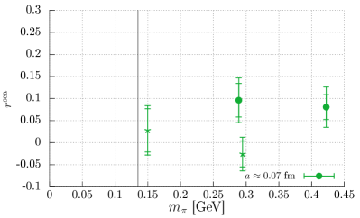
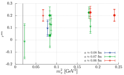
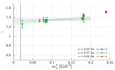
One can decompose the sigma terms further and compare sea and valence quark contributions. The ratios $a^{\rm sea}$ and $r^{\rm sea}$, shown in Fig. 16, indicate that the sea is approximately SU_F(3) symmetric, while the light quark sea accounts for less than $30\%$ of the total light quark contribution. Again, there is a fairly large spread in our results but no significant dependence on pion mass, volume or lattice spacing. Furthermore, one can look at isospin asymmetry in the form of the $z$ ratio and the $\sigma_{u}-\sigma_{d}$ difference (as a ratio with $\sigma_{\pi N}=\sigma_{u}+\sigma_{d}$), both given in Fig. 17. Here, the results are more precise and the insensitivity to the simulation parameters, in particular, the pion mass, is clear. As discussed in Section I, $z$ in combination with $\sigma_{\pi N}$ and $\sigma_{0}$ is often used in the literature to predict $f_{T_{q=u,d,s}}$. Fits to a constant and constant plus a term linear in $m_{\pi}^{2}$ in the range $m_{\pi}\lesssim 420$ MeV give values for $z$ at the physical point consistent with the results from ensemble VIII. In keeping with the analysis for $\sigma_{\pi N}$ and $\sigma_{0}$, the latter values are used for $z$ at $m_{\pi}^{\rm phys}$. We find $z=1.258(81)$, which is $3\sigma$ below the expectation of $1.49$ Cheng (1989) from the SU(3) flavour symmetry breaking of octet baryon masses. Similarly, $(\sigma_{u}-\sigma_{d})/(\sigma_{u}+\sigma_{d})=0.12(4)$ is significantly below $1/3$, obtained from simple quark counting. The physical point results for all quantities discussed above are displayed in Table 6.

V Comparison with other recent determinations of $\sigma_{\pi N}$ and $f_{T_{s}}$

Figure 18: Summary of recent lattice determinations of $\sigma_{\pi N}$ (left) and of the quark fraction $f_{T_{s}}$ (right). For $\sigma_{\pi N}$ obtained using the Feynman-Hellmann theorem we have included the work of BMW-c Dürr et al. (2012, 2015), Shanahan et al. Shanahan et al. (2013), QCDSF Horsley et al. (2012), Ren et al. Ren et al. (2012), Alvarez-Ruso et al. Alvarez-Ruso et al. (2013), Lutz and Semke Lutz and Semke (2013), Lutz et al. Lutz et al. (2014) and ETMC Alexandrou et al. (2014, 2015b). Direct determinations are displayed from QCDSF Bali et al. (2012, 2013), $\chi$QCD Yang et al. (2015a) and ETMC Abdel-Rehim et al. (2016). For $f_{T_{s}}$, the Feynman-Hellmann results shown are from BMW-c Dürr et al. (2012, 2015), Shanahan et al. Shanahan et al. (2013), QCDSF Horsley et al. (2012), Ren et al. Ren et al. (2012, 2015), JLQCD Ohki et al. (2013), Lutz and Semke Lutz and Semke (2013), Jung Jung (2012), Junnarkar and Walker-Loud Junnarkar and Walker-Loud (2013) and Lutz et al. Lutz et al. (2014). The direct evaluations were performed by QCDSF Bali et al. (2012), Freeman and Toussaint Freeman and Toussaint (2013), ETMC Dinter et al. (2012); Abdel-Rehim et al. (2016), Engelhardt Engelhardt (2012), JLQCD Ohki et al. (2013) and $\chi$QCD Gong et al. (2013); Yang et al. (2015a). RQCD refers to the present article.

In Fig. 18 we compare our results and other direct determinations of $\sigma_{\pi N}$ and $f_{T_{s}}$ with those extracted via the Feynman-Hellmann theorem. The latter indirect evaluations need to determine the slope of the nucleon mass at the physical point in terms of the light and the strange quark masses. This requires simulations which ideally include quark masses which are varied around the physical values. For light quarks this is usually missing due to the computational cost while for strange quarks the mass is normally kept fixed as the physical point is approached. A notable exception is the recent work of BMW-c Dürr et al. (2015). These problems are reflected in the larger variation in the results compared to the direct methods, in particular, for $f_{T_{s}}$. As remarked above, the direct evaluations are consistent and favour small values for $\sigma_{\pi N}\sim 35-45$ MeV and $f_{T_{s}}\lesssim 0.05$.

Alternative approaches involve the analysis of pion-nucleon scattering data. Results for $\sigma_{\pi N}$ include, for example, $45(8)$ MeV from Gasser et al. Gasser et al. (1991), $64(7)$ MeV from Pavan et al. Pavan et al. (2002), $59(7)$ MeV from Alarcon et al. Alarcón et al. (2012) and $52(7)$ MeV from Chen et al. Chen et al. (2013) and most recently $59.1(3.5)$ MeV from Hoferichter et al. Hoferichter et al. (2015a, 2016) (see also references in Hoferichter et al. (2016)). As can be seen from Fig. 18, $\sigma_{\pi N}\sim 60$ MeV is somewhat above the direct lattice results. In the Roy Steiner analysis of scattering data presented in Ref. Hoferichter et al. (2016) not only the scalar formfactor and its slope near the Cheng-Dashen (CD) point are determined but also ChPT low energy constants are obtained by matching the ChPT expressions to the sub-threshold parameters Hoferichter et al. (2015b). From the slope and the formfactor at the CD point the sigma term is estimated neglecting corrections that are formally of order $m_{\pi}^{2}/m_{N}^{2}$. The low energy constants extracted from $\pi N$ scattering data enable a detailed comparison with lattice results, also away from the physical point. In view of approximations made in some of the above analyses, the convergence of ChPT expansions at or near the physical pion mass, clearly, is of great interest.

Figure 19: (Left) Comparison of the prediction for the dependence of the nucleon mass on the pion mass provided by our determinations of $\sigma_{\pi N}$ via the Feynman-Hellmann theorem (inverse FH, the blue shaded region indicates $\pm 1\sigma$ in the parametrization) with the nucleon masses extracted from the simulation, see the text. Also shown as coloured lines are the central values of the heavy baryon ChPT predictions for $m_{N}$ up to $\mathcal{O}(m_{\pi}^{4})$ obtained using the next-to-next-to-next-to-leading order (NNNLO) low energy constants given in Ref. Hoferichter et al. (2016). (Right) A similar comparison between the pion-nucleon sigma term in the combination $(m^{\rm phys}_{\pi}/m_{\pi}^{\infty})^{2}\sigma^{\infty}_{\pi N}$ and ChPT predictions. For $\mathcal{O}(m_{\pi}^{3})$ ChPT only the central value is shown, while for $\mathcal{O}(m_{\pi}^{4})$ the uncertainty due to the error on $e_{1}$ (see Eq. (45)) is indicated by the grey shaded region. Note that we use $m_{\pi}^{\rm phys}=139.57$ MeV in the ChPT expressions (only) in keeping with Ref. Hoferichter et al. (2016).

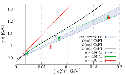
First we carry out a consistency check of our $\sigma_{\pi N}$ data, shown in Fig 19: we compare our nucleon masses (corrected for finite size effects, incorporating systematic errors, in the same way as for the sigma term) with the expectation obtained by integrating the phenomenological $(a-bm_{\pi})m_{\pi}^{2}$ parametrization of our $\sigma_{\pi N}$ values (see Section IV) as a function of $m_{\pi}^{2}$ (inverse Feynman-Hellmann method). The integration constant is adjusted so that the curve goes through the central value of the smallest pion mass point. Modulo the coarsest lattice point ($\beta=5.2$, $a=0.08$ fm) the parametrization describes the nucleon mass behaviour very well. However, it is clear from the figure that from a global fit to the nucleon mass data alone it would have been difficult to obtain the slope at the physical pion mass reliably in a parametrization independent way, unless data at smaller than physical pion masses were available. Note that such a Feynman-Hellmann study from BMW-c found $\sigma_{\pi N}=38(3)(3)$ MeV Dürr et al. (2015), in agreement with our direct evaluation.

For comparison we superimpose the heavy baryon ChPT expression used in Ref. Hoferichter et al. (2016), truncating this at different orders in $m_{\pi}^{n}$,

$$m_{N}= m_{N}^{0}-4c_{1}m_{\pi}^{2}-\frac{3g_{A}^{2}m_{\pi}^{3}}{32\pi F_{\pi}^{2}}-\frac{3}{32\pi^{2}F_{\pi}^{2}m_{N}^{0}}\left[g_{A}^{2}+m_{N}^{0}\left(-8c_{1}+c_{2}+4c_{3}\right)\right]m_{\pi}^{4}\ln\left(\frac{m_{\pi}}{m_{N}^{0}}\right)$$

$$\qquad+\left[e_{1}-\frac{3}{128\pi^{2}F_{\pi}^{2}m_{N}^{0}}\left(2g_{A}^{2}-c_{2}m_{N}^{0}\right)\right]m_{\pi}^{4}+\mathcal{O}\left(m_{\pi}^{5}\right)\,,$$ (44)

using their set of low energy constants: $c_{1}=-1.11(3)$ GeV^-1, $c_{2}=3.13(3)$ GeV^-1, $c_{3}=-5.61(6)$ GeV^-1. The value $e_{1}=11.7(4.6)$ GeV^-3 is adjusted to reproduce $\sigma_{\pi N}=59.1(3.5)$ MeV at the charged physical pion mass $m_{\pi}=139.57$ MeV and we use their determination $m_{N}^{0}=0.8695$ GeV, while $g_{A}=1.2723$ and $F_{\pi}=0.0922$ GeV are taken from experiment. The $\mathcal{O}(m_{\pi}^{4})$ curve in Fig. 19 (left) corresponds to that shown in Fig. 28 of Ref. Hoferichter et al. (2016). At least above the physical pion mass, there is disagreement between lattice data and ChPT using this set of low energy constants, also varying these (including $e_{1}$) within error bands. Note that the parametrization of our data shown in Fig. 19 gives $c_{1}=-0.51(4)$ GeV^-1. Fitting to the sigma term data, it is not possible to achieve a $c_{1}$ value of less than $-0.8$ GeV^-1.

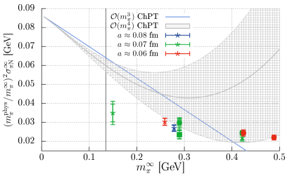
In Fig. 19 (right) the parametrization used in Ref. Hoferichter et al. (2016),

$$\sigma_{\pi N}= -4c_{1}m_{\pi}^{2}-\frac{9g_{A}^{2}m^{3}_{\pi}}{64\pi F_{\pi}^{2}}-\frac{3}{64\pi^{2}F_{\pi}^{2}m_{N}^{0}}\left[g_{A}^{2}+m_{N}^{0}\left(-8c_{1}+c_{2}+4c_{3}\right)\right]m_{\pi}^{4}\left[4\ln\left(\frac{m_{\pi}}{m_{N}^{0}}\right)+1\right]$$

$$\qquad+2\left[e_{1}-\frac{3}{128\pi^{2}F_{\pi}^{2}m_{N}^{0}}\left(2g_{A}^{2}-c_{2}m_{N}^{0}\right)+\frac{c_{1}\left(\bar{l}_{3}-1\right)}{16\pi^{2}F_{\pi}^{2}}\right]m_{\pi}^{4}+\mathcal{O}\left(m_{\pi}^{5}\right),$$ (45)

where $\bar{l}_{3}=3.41(41)$, is directly compared with our results. Unlike the nucleon mass, the sigma term is very sensitive to the value of $e_{1}$, as indicated by the shaded region in the figure. Clearly, the convergence of ChPT appears to be even inferior to that for the nucleon mass, at least for $m_{\pi}\geq m_{\pi}^{\rm phys}$. Discussions on the application of ChPT to the determination of $\sigma_{\pi N}$ can be found, for example, in Ref. Leutwyler (2015).

VI Conclusions

In summary, we performed a high statistics study of the pion and nucleon sigma terms with $N_{f}=2$ dynamical non-perturbatively improved clover fermions for pion masses ranging from $m_{\pi}\sim 500$ MeV down to close to the physical point. The set of ensembles available enabled a study of volume dependence ($Lm_{\pi}=3.42-6.71$) and, for the nucleon, also of lattice spacing effects ($a=0.06-0.08$ fm) for $m_{\pi}\gtrsim 260$ MeV. Finite volume corrections derived from ChPT turn out to be small, in particular, close to the physical point, and any remaining volume dependence could be ascribed to statistics. Similarly, for nucleon observables discretisation effects were not discernible, although leading $\mathcal{O}(a)$ terms are expected for most quantities and our lattice spacings only vary over a limited range. Extrapolations of the nucleon sigma term data using simple forms for the chiral behaviour gave consistent results with those obtained at the near physical point and we used these $m_{\pi}\sim 150$ MeV values to form the final results for quantities dominated by light quarks, such as $\sigma_{\pi N}$ and $\sigma_{q=u,d}$ for the proton in the isospin symmetric theory, summarized in Table 6. For the scalar couplings, that are expected to be less sensitive to isospin breaking effects, see Eq. (43). For the strange quark sigma terms and ratios, $\sigma_{s}$, $f_{T_{s}}$ and $y$, our results are not so precise due to large cancellations under renormalization for Wilson type fermions at our moderate lattice spacings and we quote final values obtained by extrapolation of the very mild quark mass dependence from $m_{\pi}\gtrsim 260$ MeV to the physical point.

A careful analysis procedure was implemented to extract the connected and disconnected quark line scalar matrix elements to ensure excited state contamination is minimized. In particular, for the pion this involved removing multi-pion states which propagate around the boundary and can contribute significantly if the temporal extent of the lattice is not very large. This improvement enabled us to show the GMOR expectation $\sigma_{\pi}=m_{\pi}/2$ is valid up to $m_{\pi}\sim 420$ MeV consistent with the GMOR behaviour of the pion mass as a function of the renormalized quark mass over the same range. The improvement technique may also be useful in the evaluation of other pion matrix elements.

Our study shows that with $\sigma_{\pi N}=35(6)$ MeV, the light quarks contribute very little to the mass of the nucleon. About 30$\%$ of this 3–4$\%$ fraction is due to light sea quarks. The strange quark contribution, $\sigma_{s}=35(12)$ MeV is similarly small. Appealing to the heavy quark limit, we utilized the $\alpha^{3}$ perturbative matching results Chetyrkin et al. (1998); Hill and Solon (2015a) between a theory of $N_{f}$ light quarks and one containing an additional heavy quark in order to evaluate the mass contributions from the charm, bottom and top quarks. These contributions are significantly larger than for the light and strange quarks due to the large quark masses in the combinations $m_{h}\langle\bar{h}h\rangle$. Overall, the quarks contribute about 29$\%$ of the mass, with the kinetic energies of the quarks and gluons and the anomaly accounting for $53\%$ and $18\%$, respectively, see Eq. (42). In Table 6 we also provide values for $\sigma_{0}$ and $z$. Estimates of these quantities and of $\sigma_{\pi N}$ from (non-lattice) approaches are sometimes used in the literature to predict $f_{T_{q=u,d,s}}$.

Good agreement was found for most quantities with other direct determinations involving different quark actions, pion masses, numbers of dynamical flavours, lattice spacings and volumes, in particular for $\sigma_{\pi N}$ and $f_{T_{s}}$, displayed in Fig. 18, determined around the physical point. These determinations favour small values for both quantities compared to, for example, $\sigma_{\pi N}=59.1(3.5)$ MeV from Hoferichter et al. Hoferichter et al. (2015a, 2016) from a dispersive analysis of pion-nucleon scattering data. The pion-nucleon sigma term gives the slope of the nucleon mass as a function of $m_{\pi}^{2}$ via the Feynman-Hellmann theorem. We showed our values for the sigma terms describe the nucleon mass data up to $m_{\pi}\sim 420$ MeV, providing a consistency check of the results. In contrast, the heavy baryon ChPT expansion did not seem to be well controlled above the physical point. Direct lattice calculation is the most theoretically clean approach to evaluate the sigma terms. Improvements in techniques have led to an increase in the statistical precision for $\sigma_{\pi N}$ and $f_{T_{s}}$ determined in this way and this must be accompanied by a thorough investigation of the systematics. Future calculations will involve $N_{f}=2+1$ simulations on CLS ensembles Bruno et al. (2015a) with open boundaries to remove the uncertainty of omitting the strange quark in the sea (although this is not expected to be a dominant effect) and to achieve smaller lattice spacings for which the cancellations in $f_{T_{s}}$ under renormalization are less severe. In addition, discretisation and finite volume effects will be addressed systematically also for small pion masses.

Appendix A Conventions

We work in Euclidean space-time throughout. Our continuum partition function is defined as

$$Z =\int[dA][d\bar{q}][dq]e^{-\int_{V_{4}}\!d^{4}x\mathscr{L}(x)}\,,$$ (46)

where $q$ stands for the quark flavours of the theory. Suppressing the flavour index, the Lagrangian reads

$$\mathscr{L}=\frac{1}{4}F_{\mu\nu}F_{\mu\nu}+\bar{q}\left(D_{\mu}\gamma_{\mu}+m_{q}\right)q,$$ (47)

where $D_{\mu}=\partial_{\mu}+igA_{\mu}$, $A_{\mu}=A_{\mu}^{a}t^{a}$, $F_{\mu\nu}=-\frac{i}{g}[D_{\mu},D_{\nu}]$ and $F_{\mu\nu}F_{\mu\nu}=F^{2}=F_{\mu\nu}^{a}F_{\mu\nu}^{a}$. This gives the energy-momentum tensor Freedman et al. (1974); Freedman and Weinberg (1974); Caracciolo et al. (1990)

$$T_{\mu\nu}=F_{\mu\rho}F_{\nu\rho}-\frac{1}{4}\delta_{\mu\nu}F^{2}+\frac{1}{4}\bar{q}\overleftrightarrow{D}_{\{\mu}\gamma_{\nu\}}q,$$ (48)

where $\overleftrightarrow{D}_{\mu}=\overrightarrow{D}_{\mu}-\overleftarrow{D}_{\mu}$. We define the $\beta$ function and the quark mass anomalous dimension $\gamma$-function as

$$\beta(\alpha) =\frac{d\alpha(\mu)}{d\ln\mu}=-2\alpha\left[\beta_{0}\frac{\alpha}{4\pi}+\beta_{1}\left(\frac{\alpha}{4\pi}\right)^{2}+\cdots\right],$$ (49)

$$\gamma_{m}(\alpha) =\frac{d\ln m(\mu)}{d\ln\mu}=-8\pi\left[\gamma_{0}\frac{\alpha}{4\pi}+\gamma_{1}\left(\frac{\alpha}{4\pi}\right)^{2}+\cdots\right],$$ (50)

respectively. In these conventions

$$\beta_{0}=11-\frac{2}{3}N_{f}\,,\quad\gamma_{0}=1\,.$$ (51)

The (classical plus anomalous) trace of the energy momentum tensor, i.e. the interaction measure, can be obtained as the logarithmic derivative of the free energy density with respect to a scale $M$ Coleman and Jackiw (1971); Chanowitz and Ellis (1973); Crewther (1972); Nielsen (1977); Adler et al. (1977),

$$T_{\mu\mu}=\frac{1}{V_{4}}\frac{d\ln Z}{d\ln M}=\frac{\beta(\alpha)}{\alpha}\frac{1}{4}F^{2}+\left[\gamma_{m}(\alpha)-1\right]m_{q}\bar{q}q.$$ (52)

Note that the covariant derivative is independent of the coupling. Rescaling $gA_{\mu}\mapsto A_{\mu}$ makes this explicit. As $F^{2}/4=-(16\pi\alpha)^{-1}[D_{\mu},D_{\nu}][D_{\mu},D_{\nu}]$ with $\alpha=g^{2}/(4\pi)$, the derivative of the gluon kinetic term gives $-\beta(\alpha)/(4\alpha)F^{2}$. The anomalous quark mass dimension is obtained from applying the Leibniz rule to the derivative of the combination $(m/M)\left(M\int\!d^{4}x\,\bar{q}q\right)$.

We decompose $T_{\mu\nu}=\overline{T}_{\mu\nu}+\hat{T}_{\mu\nu}$, where $\overline{T}$ is traceless and

$$\hat{T}_{\mu\nu}=\frac{1}{4}\delta_{\mu\nu}T_{\rho\rho}.$$ (53)

With $F^{2}=2(\mathbf{E}^{2}+\mathbf{B}^{2})$, $F_{4\mu}F_{4\mu}=\mathbf{E}^{2}$ and using the equations of motion for the quark fields, this gives

$$\overline{T}_{44}=\frac{1}{2}\left(\mathbf{E}^{2}-\mathbf{B}^{2}\right)-\bar{q}\boldsymbol{D}\cdot\boldsymbol{\gamma}q-\frac{3}{4}m_{q}\bar{q}{q},$$ (54)

where $-\frac{1}{4}m_{q}\bar{q}q$ is the classical contribution to $\hat{T}_{44}$. Note that $-T_{44}$ is the energy density.

Within Eq. (52) the combinations

$$m_{q}\bar{q}q\,,\quad\frac{\beta(\alpha)}{4\alpha}F^{2}+\gamma_{m}(\alpha)m_{q}\bar{q}q,$$ (55)

taken between physical states, are both renormalization group invariants (RGI), however, the second term is discontinuous at flavour thresholds. Note that this term, multiplied by $-8/\beta_{0}$ gives the combination whose vacuum expectation value is known as the RGI definition of the non-perturbative gluon condensate Tarrach (1982). The scale independence of the two contributions shown in Eq. (55) enables, within the heavy quark approximation, the matching of a theory of $N_{f}$ quark flavours at a scale $M<m_{h}$ to a theory of $N_{f}$ light flavours plus one heavy flavour of mass $m_{h}$ at a scale $M>m_{h}$ Shifman et al. (1978).

Appendix B Spectral decomposition of the pion two- and three-point functions

In order to motivate our method for reducing excited state contributions and the subsequent choice of fit forms we start with the transfer matrix expressions for $C_{{\rm 2pt}}$ and $C_{{\rm 3pt}}$ in Eqs. (14) and (15), respectively, with periodic boundary conditions:

$$C_{{\rm 2pt}}(t_{\mathrm{f}},0)= \frac{1}{Z(T)}\mathrm{Tr}\left[e^{-(T-t_{\rm f})\hat{H}}{\cal H}(0)e^{-t_{\rm f}\hat{H}}{\overline{\cal H}}(0)\right]=\sum_{n,m}\langle n|{\cal H}(0)|m\rangle\langle m|{\cal\overline{H}}(0)|n\rangle e^{-(T-t_{\rm f})E_{n}}e^{-t_{\rm f}E_{m}},$$ (56)

$$C_{{\rm 3pt}}(t_{\mathrm{f}},t,0)= \frac{1}{Z(T)}\mathrm{Tr}\left[e^{-(T-t_{\rm f})\hat{H}}{\cal H}(0)e^{-(t_{\rm f}-t)\hat{H}}S(0)e^{-t\hat{H}}{\overline{\cal H}}(0)\right]$$

$$-\frac{1}{Z(T)}\mathrm{Tr}\left[e^{-(T-t)\hat{H}}S(0)e^{-t\hat{H}}\right]\frac{1}{Z(T)}\mathrm{Tr}\left[e^{-(T-t_{\rm f})\hat{H}}{\cal H}(0)e^{-t_{\rm f}\hat{H}}{\overline{\cal H}}(0)\right]$$ (57)

$$= \sum_{k,n,m}\langle n|{\cal H}(0)|m\rangle\langle m|S(0)|k\rangle\langle k|{\cal\overline{H}}(0)|n\rangle e^{-(T-t_{\rm f})E_{n}}e^{-(t_{\rm f}-t)E_{m}}e^{-tE_{k}}$$

$$-\left[\sum_{n}\langle n|S(0)|n\rangle e^{-TE_{n}}\right]\left[\sum_{n,m}\langle n|{\cal H}(0)|m\rangle\langle m|{\cal\overline{H}}(0)|n\rangle e^{-(T-t_{\rm f})E_{n}}e^{-t_{\rm f}E_{m}}\right],$$ (58)

where $\hat{H}$ is the lattice Hamiltonian and $Z(T)=\langle 0|e^{-T\hat{H}}|0\rangle$ the partition function. For convenience, we assume that the source time $t_{\rm i}=0$ and ${\cal H}(t)=\sum_{\vec{x}}{\cal H}(\vec{x},t)$. For an interpolator ${\cal H}=\bar{u}\gamma_{5}d$ with pseudoscalar quantum numbers, $J^{P}=0^{-}$, the overlap matrix $\langle n|{\cal H}(0)|m\rangle$ can link any (single- or multi-particle) states $|n\rangle$ and $|m\rangle$ with $J=0$ if and only if the states have opposite parity and $\Delta I=1$. Similarly, the matrix element $\langle n|S(0)|m\rangle$ for the scalar operator $S=\bar{q}q$ is non-zero for $n$ and $m$ with the same parity, $J$, isospin and strangeness. We denote the even states, $|0\rangle,|2\rangle,|4\rangle,\ldots$ and the odd states, $|1\rangle,|3\rangle,|5\rangle\ldots$, where $|0\rangle$ represents the vacuum and $|1\rangle$ the ground state pion. Since the lowest lying single-particle $0^{+}$ state is heavier in mass than $2m_{\pi}$ and the radially excited pion lies above 1 GeV then $|n\rangle$ can be thought of as an $n$-pion multi-particle state for small $n$. Considering only $n\leq 2$ to begin with, the spectral decompositions are given by

$$C_{{\rm 2pt}}(t_{\mathrm{f}},0) =|Z_{01}|^{2}e^{-t_{\rm f}E_{1}}\left\{1+e^{-(T-2t_{\rm f})E_{1}}+\frac{|Z_{12}|^{2}}{|Z_{01}|^{2}}\left[e^{-(T-t_{\rm f})E_{2}}+e^{-t_{\rm f}E_{2}}e^{-(T-2t_{\rm f})E_{1}}\right]\right\},$$ (59)

$$C_{{\rm 3pt}}(t_{\mathrm{f}},t,0) =|Z_{01}|^{2}e^{-t_{\rm f}E_{1}}\left\{\langle 1|S|1\rangle_{\rm sub}+\frac{|Z_{12}|^{2}}{|Z_{01}|^{2}}\left(\langle 1|S|1\rangle_{\rm sub}e^{-(T-t_{\rm f})E_{2}}+\langle 2|S|2\rangle_{\rm sub}e^{-(T-2t_{\rm f})E_{1}}e^{-t_{\rm f}E_{2}}\right)\right.$$

$$+\left.\frac{Z^{*}_{01}Z_{21}}{|Z_{01}|^{2}}\langle 0|S|2\rangle e^{-(T-2t_{\rm f})E_{1}}\left(e^{-tE_{2}}+e^{-(t_{\rm f}-t)E_{2}}\right)\right.$$

$$-\left(\langle 1|S|1\rangle e^{-TE_{1}}+\langle 2|S|2\rangle e^{-TE_{2}}\right)\left.\left(1+e^{-(T-2t_{\rm f})E_{1}}+\frac{|Z_{21}|^{2}}{|Z_{01}|^{2}}\left[e^{-t_{\rm f}E_{1}}e^{-(T-t_{\rm f})E_{2}}+e^{-t_{\rm f}E_{2}}e^{-(T-t_{\rm f})E_{1}}\right]\right)\right\},$$ (60)

for $T>t_{\rm f}>t>0$, where $\langle n|S|n\rangle_{\rm sub}=\langle n|S|n\rangle-\langle 0|S|0\rangle$, the overlap $Z_{nm}=Z_{mn}^{*}=\langle n|{\cal\overline{H}}(0)|m\rangle$ and $E_{n}\approx nE_{1}$ is the energy of state $|n\rangle$. Note that the expressions above are relevant for correlators generated with the same source and sink interpolator, for example, smeared-smeared (SS) two- and three-point functions. Corrections to ground state dominance involve terms arising from a forward propagating pion state together with a scalar (two-pion) state propagating backward around the temporal boundary and vice versa. Depending on the size of the overlaps and matrix elements, some of the terms in Eq. (60) can be large for $t_{\rm f}\gtrsim T/2$, in particular since $E_{2}$ is rather small, for example, $2am_{\pi}\approx 0.11$ for ensemble VIII in Table 2.

Contributions involving an odd parity state propagating across the boundary in the backward direction can be removed by constructing correlation functions from quark propagators with different boundary conditions in time. For example, the two-point function with the spectral decomposition of Eq. (59) is computed using

$$C_{{\rm 2pt}}(t_{\mathrm{f}},0)=\sum_{\vec{x}}\mathrm{Tr}\left[(M^{-1})^{\dagger}(\vec{x},t_{\rm f};\vec{0},0)M^{-1}(\vec{x},t_{\rm f};\vec{0},0)\right],$$ (61)

where both propagators, $M^{-1}(\vec{x},t_{\rm f};\vec{0},0)$, have anti-periodic boundary conditions (AP) in time imposed. If instead one of the propagators has periodic boundary conditions (P), then the two-point function for this AP-P combination will change sign when crossing the temporal boundary. This choice corresponds to the H-boundary condition of Ref. Kim (2004) that had been used in earlier studies of nucleon excited states Sasaki et al. (2002). Such boundary effects were first discussed in Ref. Martinelli et al. (1983). Returning to Eq. (56) and separating the terms into two sums gives:

$$C_{{\rm 2pt}}(t_{\mathrm{f}},0)=\left(\sum_{n\,\,{\rm even},\,m\,\,{\rm odd}}+\sum_{n\,\,{\rm odd},\,m\,\,{\rm even}}\right)\langle n|{\cal H}(0)|m\rangle\langle m|{\cal\overline{H}}(0)|n\rangle e^{-(T-t_{\rm f})E_{n}}e^{-t_{\rm f}E_{m}}.$$ (62)

The AP-P two-point function, $C_{{\rm 2pt}}^{\rm AP-P}$, will have a minus sign for the second sum relative to $C_{{\rm 2pt}}^{\rm AP-AP}$. Taking the average of these, we obtain the forward propagating odd parity states only:

$$C^{\rm improv}_{{\rm 2pt}}(t_{\mathrm{f}},0)=\frac{1}{2}\left[C^{\rm AP-P}_{{\rm 2pt}}(t_{\mathrm{f}},0)+C^{\rm AP-AP}_{{\rm 2pt}}(t_{\mathrm{f}},0)\right] =|Z_{01}|^{2}e^{-t_{\rm f}E_{1}}\left[1+\frac{|Z_{12}|^{2}}{|Z_{01}|^{2}}e^{-(T-t_{\rm f})E_{2}}+\ldots\right].$$ (63)

The same effect can be achieved for the three-point function by combining both AP and P quark propagators:

$$C^{\rm improv}_{{\rm 3pt}}(t_{\mathrm{f}},t,0) =\frac{1}{2}\left[C^{AP-P}_{{\rm 3pt}}(t_{\mathrm{f}},t,0)+C^{AP-AP}_{{\rm 3pt}}(t_{\mathrm{f}},t,0)\right].$$ (64)

For the disconnected part this corresponds to

$$C^{\rm improv,dis}_{{\rm 3pt}}(t_{\mathrm{f}},t,0)=\langle C^{\rm improv,c}_{{\rm 2pt}}(t_{\mathrm{f}},0)L^{c}(t)\rangle_{c},$$ (65)

cf. Eq. (16), where the loop is constructed from a propagator with AP boundary conditions, $(M^{-1})^{\rm AP}$, while for the connected part,

$$C^{\rm improv,conn}_{{\rm 3pt}}(t_{\mathrm{f}},t,0)= \frac{1}{2}\left\{\langle\mathrm{Tr}\left[(M^{-1})^{\rm P\dagger}(t_{\rm f},0)(M^{-1})^{\rm AP}(t_{\rm f};t)(M^{-1})^{\rm AP}(t;0)\right]\rangle\right.$$

$$\left.+\langle\mathrm{Tr}\left[(M^{-1})^{\rm AP\dagger}(t_{\rm f},0)(M^{-1})^{\rm AP}(t_{\rm f};t)(M^{-1})^{\rm AP}(t;0)\right]\rangle\right\}.$$ (66)

The improved three-point function has the spectral decomposition

$$C^{\rm improv}_{{\rm 3pt}}(t_{\mathrm{f}},t,0) =|Z_{01}|^{2}e^{-t_{\rm f}E_{1}}\left[1+\frac{|Z_{12}|^{2}}{|Z_{01}|^{2}}e^{-(T-t_{\rm f})E_{2}}+\ldots\right]\left[\langle 1|S|1\rangle_{\rm sub}-\langle 1|S|1\rangle e^{-TE_{1}}-\langle 2|S|2\rangle e^{-TE_{2}}-\ldots\right],$$ (67)

$$\approx|Z_{01}|^{2}e^{-t_{\rm f}E_{1}}\left[1+\frac{|Z_{12}|^{2}}{|Z_{01}|^{2}}e^{-(T-t_{\rm f})E_{2}}+\ldots\right]\langle 1|S|1\rangle_{\rm sub}.$$ (68)

In the last step we neglect the terms with factors, $e^{-TE_{1}}$ and $e^{-TE_{2}}$, which are $e^{-TE_{1}}<0.03$ and $e^{-TE_{2}}<0.001$, respectively, for the ensembles in Table 1. These limits are calculated using $E_{2}=2m_{\pi}$ and the smallest value for $Tm_{\pi}\sim 3.5$ (obtained from ensemble VIII). Note that such terms can be significant in finite temperature studies Umeda (2007), where, however, the use of AP boundary conditions is mandatory.

In some cases in our study the improved three-point functions still contain significant contributions from the next state (the forward propagating $|3\rangle$ state). Including the appropriate terms, we have

$$C^{\rm improv}_{{\rm 2pt}}(t_{\mathrm{f}},0) =|Z_{01}|^{2}e^{-t_{\rm f}E_{1}}\left[1+\frac{|Z_{21}|^{2}}{|Z_{01}|^{2}}e^{-(T-t_{\rm f})E_{2}}+\frac{|Z_{03}|^{2}}{|Z_{01}|^{2}}e^{-t_{\rm f}\Delta E}+\ldots\right]$$ (69)

$$\approx|Z_{01}|^{2}e^{-t_{\rm f}E_{1}}\left[1+\frac{|Z_{03}|^{2}}{|Z_{01}|^{2}}e^{-t_{\rm f}\Delta E}\right],$$ (70)

$$C^{\rm improv}_{{\rm 3pt}}(t_{\mathrm{f}},t,0) =|Z_{01}|^{2}e^{-t_{\rm f}E_{1}}\left[\langle 1|S|1\rangle_{\rm sub}\left(1+\frac{|Z_{21}|^{2}}{|Z_{01}|^{2}}e^{-(T-t_{\rm f})E_{2}}\right)\right.$$

$$\left.+\frac{|Z_{03}|^{2}}{|Z_{01}|^{2}}\langle 3|S|3\rangle_{\rm sub}e^{-t_{\rm f}\Delta E}+\frac{Z^{*}_{10}Z_{30}}{|Z_{01}|^{2}}\langle 1|S|3\rangle\left(e^{-(t_{\rm f}-t)\Delta E}+e^{-t\Delta E}\right)+\ldots\right],$$ (71)

$$\approx|Z_{01}|^{2}e^{-t_{\rm f}E_{1}}\left[\langle 1|S|1\rangle_{\rm sub}+\frac{|Z_{03}|^{2}}{|Z_{01}|^{2}}\langle 3|S|3\rangle_{\rm sub}e^{-t_{\rm f}\Delta E}\right.\left.+\frac{Z^{*}_{10}Z_{30}}{|Z_{01}|^{2}}\langle 1|S|3\rangle\left(e^{-(t_{\rm f}-t)\Delta E}+e^{-t\Delta E}\right)\right],$$ (72)

in the limit $t_{\rm f}\ll T$, where $e^{-(T-t_{\rm f})E_{2}}\sim 0$. $\Delta E$ denotes the difference $E_{3}-E_{1}$. We also compute the ratio of the improved three-point and two-point functions. If the excited state contribution to $C^{\rm improv}_{{\rm 2pt}}$ is small, the ratio has the time dependence

$$R^{\rm improv}(t_{\mathrm{f}},t,0)\approx \langle 1|S|1\rangle^{\rm dis}_{\rm sub}+\frac{|Z_{03}|^{2}}{|Z_{01}|^{2}}\left[\langle 3|S|3\rangle_{\rm sub}-\langle 1|S|1\rangle_{\rm sub}\right]e^{-t_{\rm f}\Delta E}+\frac{Z^{*}_{30}Z_{10}}{|Z_{01}|^{2}}\langle 3|S|1\rangle\left(e^{-(t_{\rm f}-t)\Delta E}+e^{-t\Delta E}\right),$$ (73)

where terms with factors, $e^{-2t_{\rm f}\Delta E}$ and $e^{-(t_{\rm f}+t)\Delta E}$ and smaller are not included. For our data these assumptions are reasonable as demonstrated in Fig. 4 which shows the deviation of improved two-point functions from ground state dominance for ensembles with $m_{\pi}=289$ MeV and $m_{\pi}=150$ MeV. Excited state contributions are small and drop below the noise for $t_{\rm f}\lesssim 10a$.

The connected and disconnected contributions to the three-point function are analysed individually. Equations (60), (68), (72) and (73) give the functional forms of the disconnected part, which includes the subtraction of $\langle 0|S|0\rangle$. For the connected part the expressions are similar and can be obtained by replacing $\langle n|S|n\rangle_{\rm sub}$ by $\langle n|S|n\rangle$ for $n=1,2,3$. Also in Eq. (60) the subtracted term in the last line is not present.

Finally, if different interpolators are employed at source and sink, for example, connected or disconnected three-point functions that are smeared at the source and local at the sink, then one cannot simplify,

$$\frac{Z^{*}_{30}Z_{10}}{|Z_{01}|^{2}}\langle 3|S|1\rangle e^{-(t_{\rm f}-t)\Delta E}+\frac{Z^{*}_{10}Z_{30}}{|Z_{01}|^{2}}\langle 1|S|3\rangle e^{-t\Delta E}$$

$$=\frac{Z^{*}_{30}Z_{10}}{|Z_{01}|^{2}}\langle 3|S|1\rangle\left[e^{-(t_{\rm f}-t)\Delta E}+e^{-t\Delta E}\right],$$ (74)

and similarly in Eqs. (60), (68), (72) and (73). Accordingly, in this case the functional forms must be modified to allow for different coefficients for these pairs of terms.

Appendix C Finite volume corrections to the nucleon and pion sigma terms

For convenience we collect the expressions used for applying finite volume corrections to the pion and nucleon sigma terms. For the pion we use NLO ChPT Gasser and Leutwyler (1987, 1988),

$$m_{\pi}(L) =m_{\pi}\left[1+\frac{2}{N_{f}}\frac{m_{\pi}^{2}}{16\pi^{2}F^{2}}I(\lambda)\right],$$ (75)

with

$$I(\lambda)=\sum_{\vec{n}}\frac{K_{1}(\lambda|\vec{n}|)}{\lambda|\vec{n}|},$$ (76)

where $\lambda=Lm_{\pi}$, $K_{1}$ is the modified Bessel function of the second kind and $\vec{n}\neq\vec{0}$ is an integer valued vector. Using the Feynman-Hellmann theorem and the GMOR relation we have for the finite volume pion sigma term, $\sigma_{\pi}(L)=2\sigma_{u}(L)=2\sigma_{d}(L)$,

$$\sigma_{\pi}(L) =\left.\frac{1}{m_{\pi}(L)}\frac{\partial m_{\pi}^{2}(L)}{\partial\ln m_{u}}\right|_{L\,\,\mathrm{fixed}}=\left.\sigma_{\pi}\frac{\partial m_{\pi}(L)}{\partial m_{\pi}}\right|_{L\,\,\mathrm{fixed}}$$ (77)

$$=\sigma_{\pi}\left[1+\frac{2}{N_{f}}\frac{m_{\pi}^{2}}{16\pi^{2}F^{2}}\left(3I(\lambda)+\lambda\frac{dI(\lambda)}{d\lambda}\right)\right],$$ (78)

where $F$, $m_{\pi}$ and $\sigma_{\pi}$ are the pion decay constant, pion mass and sigma term in the infinite volume limit, respectively. We can then invert the equation above, truncating at $\mathcal{O}(m_{\pi}^{2})$:

$$\sigma_{u} =\sigma_{u}(L)\left[1-\frac{2}{N_{f}}\frac{m_{\pi}^{2}}{16\pi^{2}F^{2}}\left(3I(\lambda)+\lambda\frac{dI(\lambda)}{d\lambda}\right)\right].$$ (79)

For the nucleon we again use NLO ChPT, see, for example, Ref. Ali Khan et al. (2004):

$$m_{N}(L) =m_{N}\left[1+\frac{3g_{A}^{2}m_{\pi}^{2}}{16\pi^{2}F^{2}}I_{0}(\lambda,m_{N}/m_{\pi})\right],$$ (80)

where

$$I_{0}(\lambda,m_{N}/m_{\pi}) =\int_{0}^{\infty}\!\!dx\sum_{\vec{n}}K_{0}\left(\lambda|\vec{n}|\sqrt{\frac{m_{N}^{2}}{m_{\pi}^{2}}x^{2}+1-x}\right).$$ (81)

With the Feynman-Hellmann theorem and the GMOR relation,

$$\sigma_{\pi N}(L) =\left.\frac{\partial m_{N}(L)}{\partial\ln m_{\ell}}\right|_{L\,\,\mathrm{fixed}}\approx\left.m_{\pi}^{2}\frac{\partial m_{N}(L)}{\partial m_{\pi}^{2}}\right|_{L\,\,\mathrm{fixed}},$$ (82)

this leads to

$$\sigma_{\pi N}(L) =\sigma_{\pi N}+\frac{3g_{A}^{2}m_{\pi}^{2}}{16\pi^{2}F^{2}}\left[(\sigma_{\pi N}+m_{N})I_{0}(\lambda,m_{N}/m_{\pi})\right.$$

$$\left.\qquad+m_{N}I_{1}(\lambda,m_{N}/m_{\pi})\right],$$ (83)

where

$$I_{1}(\lambda,m_{N}/m_{\pi}) =\int_{0}^{\infty}dx\frac{x-1}{2\sqrt{\frac{m_{N}^{2}}{m_{\pi}^{2}}x^{2}+1-x}}\sum_{\vec{n}}\lambda|\vec{n}|K_{1}\left(\lambda|\vec{n}|\sqrt{\frac{m_{N}^{2}}{m_{\pi}^{2}}x^{2}+1-x}\right).$$ (84)

Inverting the above formula and truncating at $\mathcal{O}(m_{\pi}^{2})$, we obtain

$$\sigma_{\pi N} =\sigma_{\pi N}(L)-\frac{3g_{A}^{2}m_{\pi}^{2}}{16\pi^{2}F^{2}}\left[(\sigma_{\pi N}(L)+m_{N})I_{0}(\lambda,m_{N}/m_{\pi})+m_{N}I_{1}(\lambda,m_{N}/m_{\pi})\right].$$ (85)

For the corrections to both the pion and nucleon sigma terms we estimate the error of the finite volume shifts to be half the size of the correction applied. This is added in quadrature to the statistical and the other systematic uncertainties.

The above formulae entail the pion mass in infinite volume. This is obtained using the largest available volume for each $(\beta,\kappa)$ combination, the NNNLO analytic expressions of Ref. Colangelo et al. (2005) and the low energy constants of Refs. Colangelo et al. (2005); Aoki et al. (2014), see Ref. Bali et al. (2015) for details.

References

- Shifman et al. (1978) Mikhail A. Shifman, Arkady I. Vainshtein, and Valentin I. Zakharov, “Remarks on Higgs Boson Interactions with Nucleons,” Phys. Lett. B78, 443 (1978).
- Ji (1995a) Xiang-Dong Ji, “A QCD analysis of the mass structure of the nucleon,” Phys. Rev. Lett. 74, 1071 (1995a), arXiv:hep-ph/9410274 [hep-ph] .
- Ji (1995b) Xiang-Dong Ji, “Breakup of hadron masses and the energy-momentum tensor of QCD,” Phys. Rev. D52, 271 (1995b), arXiv:hep-ph/9502213 [hep-ph] .
- Cline et al. (2013) James M. Cline, Kimmo Kainulainen, Pat Scott, and Christoph Weniger, “Update on scalar singlet dark matter,” Phys. Rev. D88, 055025 (2013), arXiv:1306.4710 [hep-ph] .
- Hietanen et al. (2014) Ari Hietanen, Randy Lewis, Claudio Pica, and Francesco Sannino, “Composite Goldstone Dark Matter: Experimental Predictions from the Lattice,” JHEP 12, 130 (2014), arXiv:1308.4130 [hep-ph] .
- Hill and Solon (2015a) Richard J. Hill and Mikhail P. Solon, “Standard Model anatomy of WIMP dark matter direct detection II: QCD analysis and hadronic matrix elements,” Phys. Rev. D91, 043505 (2015a), arXiv:1409.8290 [hep-ph] .
- Hill and Solon (2015b) Richard J. Hill and Mikhail P. Solon, “Standard Model anatomy of WIMP dark matter direct detection I: weak-scale matching,” Phys. Rev. D91, 043504 (2015b), arXiv:1401.3339 [hep-ph] .
- Ellis et al. (2016) John Ellis, Jason L. Evans, Feng Luo, Natsumi Nagata, Keith A. Olive, and Pearl Sandick, “Beyond the CMSSM without an Accelerator: Proton Decay and Direct Dark Matter Detection,” Eur. Phys. J. C76, 8 (2016), arXiv:1509.08838 [hep-ph] .
- Abdallah et al. (2015) Jalal Abdallah et al., “Simplified Models for Dark Matter Searches at the LHC,” Phys. Dark Univ. 9-10, 8 (2015), arXiv:1506.03116 [hep-ph] .
- Gasser et al. (1991) Jürg Gasser, Heinrich Leutwyler, and Mikko E. Sainio, “Sigma term update,” Phys. Lett. B253, 252 (1991).
- Pavan et al. (2002) Marcello M. Pavan, Igor I. Strakovsky, Ron L. Workman, and Richard A. Arndt, “The Pion nucleon Sigma term is definitely large: Results from a G.W.U. analysis of pi nucleon scattering data,” Meson nucleon physics and the structure of the nucleon. Proceedings, 9th International Symposium, MENU 2001, Washington, USA, July 26-31, 2001, PiN Newslett. 16, 110 (2002), arXiv:hep-ph/0111066 [hep-ph] .
- Alarcón et al. (2013) Jose M. Alarcón, Jorge Martin Camalich, and Jose A. Oller, “Improved description of the -scattering phenomenology in covariant baryon chiral perturbation theory,” Annals Phys. 336, 413 (2013), arXiv:1210.4450 [hep-ph] .
- Hoferichter et al. (2015a) Martin Hoferichter, Jacobo Ruiz de Elvira, Bastian Kubis, and Ulf-G. Meißner, “High-Precision Determination of the Pion-Nucleon σ Term from Roy-Steiner Equations,” Phys. Rev. Lett. 115, 092301 (2015a), arXiv:1506.04142 [hep-ph] .
- Hoferichter et al. (2016) Martin Hoferichter, Jacobo Ruiz de Elvira, Bastian Kubis, and Ulf-G. Meißner, “Roy–Steiner-equation analysis of pion–nucleon scattering,” Phys. Rept. 625, 1 (2016), arXiv:1510.06039 [hep-ph] .
- Yang et al. (2015a) Yi-Bo Yang, Andrei Alexandru, Terrence Draper, Jian Liang, and Keh-Fei Liu (QCD Collaboration), “N and strangeness sigma terms at the physical point with chiral fermions,” (2015a), arXiv:1511.09089 [hep-lat] .
- Abdel-Rehim et al. (2016) Abdou Abdel-Rehim, Constantia Alexandrou, Martha Constantinou, Kyriakos Hadjiyiannakou, Karl Jansen, Christos Kallidonis, Giannis Koutsou, and Alejandro Vaquero Aviles-Casco (ETM Collaboration), “Direct evaluation of the quark content of the nucleon from lattice QCD at the physical point,” (2016), arXiv:1601.01624 [hep-lat] .
- Freedman et al. (1974) Daniel Z. Freedman, Ivan J. Muzinich, and Erick J. Weinberg, “On the Energy-Momentum Tensor in Gauge Field Theories,” Annals Phys. 87, 95 (1974).
- Freedman and Weinberg (1974) Daniel Z. Freedman and Erick J. Weinberg, “The Energy-Momentum Tensor in Scalar and Gauge Field Theories,” Annals Phys. 87, 354 (1974).
- Caracciolo et al. (1990) Sergio Caracciolo, Giuseppe Curci, Pietro Menotti, and Andrea Pelissetto, “The Energy Momentum Tensor for Lattice Gauge Theories,” Annals Phys. 197, 119 (1990).
- Coleman and Jackiw (1971) Sidney R. Coleman and Roman Jackiw, “Why dilatation generators do not generate dilatations?” Annals Phys. 67, 552 (1971).
- Chanowitz and Ellis (1973) Michael S. Chanowitz and John R. Ellis, “Canonical Trace Anomalies,” Phys. Rev. D7, 2490 (1973).
- Crewther (1972) Rodney J. Crewther, “Nonperturbative evaluation of the anomalies in low-energy theorems,” Phys. Rev. Lett. 28, 1421 (1972).
- Nielsen (1977) Niels K. Nielsen, “The Energy Momentum Tensor in a Nonabelian Quark Gluon Theory,” Nucl. Phys. B120, 212 (1977).
- Adler et al. (1977) Stephen L. Adler, John C. Collins, and Anthony Duncan, “Energy-Momentum-Tensor Trace Anomaly in Spin 1/2 Quantum Electrodynamics,” Phys. Rev. D15, 1712 (1977).
- Tarrach (1982) Rolf Tarrach, “The Renormalization of FF,” Nucl. Phys. B196, 45 (1982).
- Cheng (1989) Hai-Yang Cheng, “Low-energy Interactions of Scalar and Pseudoscalar Higgs Bosons With Baryons,” Phys. Lett. B219, 347 (1989).
- Donoghue et al. (1990) John F. Donoghue, Jürg Gasser, and Heinrich Leutwyler, “The Decay of a Light Higgs Boson,” Nucl. Phys. B343, 341 (1990).
- Ananthanarayan et al. (2004) Balasubramanian Ananthanarayan, Irinel Caprini, Gilberto Colangelo, Jürg Gasser, and Heinrich Leutwyler, “Scalar form-factors of light mesons,” Phys. Lett. B602, 218 (2004), arXiv:hep-ph/0409222 [hep-ph] .
- Yang et al. (2015b) Yi-Bo Yang, Ying Chen, Terrence Draper, Ming Gong, Keh-Fei Liu, Zhaofeng Liu, and Jian-Ping Ma, “Meson Mass Decomposition from Lattice QCD,” Phys. Rev. D91, 074516 (2015b), arXiv:1405.4440 [hep-ph] .
- Vecchi (2013) Luca Vecchi, “WIMPs and Un-Naturalness,” (2013), arXiv:1312.5695 [hep-ph] .
- Bali et al. (2014) Gunnar S. Bali, Sara Collins, Benjamin Gläßle, Meinulf Göckeler, Johannes Najjar, Rudolf H. Rödl, Andreas Schäfer, Rainer W. Schiel, André Sternbeck, and Wolfgang Söldner, “The moment of the nucleon from lattice QCD down to nearly physical quark masses,” Phys. Rev. D 90, 074510 (2014), arXiv:1408.6850 [hep-lat] .
- Bali et al. (2013) Gunnar S. Bali et al., “Nucleon mass and sigma term from lattice QCD with two light fermion flavors,” Nucl. Phys. B866, 1 (2013), arXiv:1206.7034 [hep-lat] .
- Bhattacharya et al. (2006) Tanmoy Bhattacharya, Rajan Gupta, Weonjong Lee, Stephen R. Sharpe, and Jackson M. S. Wu, “Improved bilinears in lattice QCD with non-degenerate quarks,” Phys. Rev. D73, 034504 (2006), arXiv:hep-lat/0511014 [hep-lat] .
- Bali et al. (2015) Gunnar S. Bali, Sara Collins, Benjamin Gläßle, Meinulf Göckeler, Johannes Najjar, Rudolf H. Rödl, Andreas Schäfer, Rainer W. Schiel, Wolfgang Söldner, and Andre Sternbeck, “Nucleon isovector couplings from lattice QCD,” Phys. Rev. D91, 054501 (2015), arXiv:1412.7336 [hep-lat] .
- Bruno et al. (2015a) Mattia Bruno et al., “Simulation of QCD with N 2 1 flavors of non-perturbatively improved Wilson fermions,” JHEP 02, 043 (2015a), arXiv:1411.3982 [hep-lat] .
- Güsken et al. (1989) Stephan Güsken, Ute Löw, Karl-Heinz Mütter, Rainer Sommer, Apoorva D. Patel, and Klaus Schilling, “Nonsinglet Axial Vector Couplings of the Baryon Octet in Lattice QCD,” Phys. Lett. B227, 266 (1989).
- Güsken (1990) Stephan Güsken, “A Study of smearing techniques for hadron correlation functions,” Nucl. Phys. B Proc. Suppl. 17, 361 (1990).
- Falcioni et al. (1985) Massimo Falcioni, Maria L. Paciello, Giorgio Parisi, and Bruno Taglienti, “Again on SU(3) glueball mass,” Nucl. Phys. B251, 624 (1985).
- Bali et al. (2010) Gunnar S. Bali, Sara Collins, and Andreas Schäfer, “Effective noise reduction techniques for disconnected loops in Lattice QCD,” Comput. Phys. Commun. 181, 1570 (2010), arXiv:0910.3970 [hep-lat] .
- Bali et al. (2012) Gunnar S. Bali et al. (QCDSF), “The strange and light quark contributions to the nucleon mass from Lattice QCD,” Phys. Rev. D85, 054502 (2012), arXiv:1111.1600 [hep-lat] .
- Fritzsch et al. (2010) Patrick Fritzsch, Jochen Heitger, and Nazario Tantalo, “Non-perturbative improvement of quark mass renormalization in two-flavour lattice QCD,” JHEP 08, 074 (2010), arXiv:1004.3978 [hep-lat] .
- Göckeler et al. (2006) Meinulf Göckeler, Roger Horsley, Alan C. Irving, Dirk Pleiter, Paul E. L. Rakow, Gerrit Schierholz, Hinnerk Stüben, and James M. Zanotti (QCDSF and UKQCD Collaborations), “Estimating the unquenched strange quark mass from the lattice axial Ward identity,” Phys. Rev. D73, 054508 (2006), arXiv:hep-lat/0601004 [hep-lat] .
- (43) Dirk Pleiter, private communication.
- Fritzsch et al. (2012) Patrick Fritzsch, Francesco Knechtli, Bjorn Leder, Marina Marinkovic, Stefan Schaefer, Rainer Sommer, and Francesco Virotta, “The strange quark mass and Lambda parameter of two flavor QCD,” Nucl. Phys. B865, 397 (2012), arXiv:1205.5380 [hep-lat] .
- Colangelo et al. (2005) Gilberto Colangelo, Stephan Dürr, and Christoph Haefeli, “Finite volume effects for meson masses and decay constants,” Nucl. Phys. B721, 136 (2005), arXiv:hep-lat/0503014 [hep-lat] .
- Gasser and Leutwyler (1987) Jürg Gasser and Heinrich Leutwyler, “Light Quarks at Low Temperatures,” Phys. Lett. B184, 83 (1987).
- Gasser and Leutwyler (1988) Jürg Gasser and Heinrich Leutwyler, “Spontaneously Broken Symmetries: Effective Lagrangians at Finite Volume,” Nucl. Phys. B 307, 763 (1988).
- Ali Khan et al. (2004) Arifa Ali Khan et al. (QCDSF and UKQCD Collaborations), “The Nucleon mass in = 2 lattice QCD: Finite size effects from chiral perturbation theory,” Nucl. Phys. B689, 175 (2004), arXiv:hep-lat/0312030 [hep-lat] .
- Dinter et al. (2012) Simon Dinter, Vincent Drach, Roberto Frezzotti, Gregorio Herdoiza, Karl Jansen, and Giancarlo Rossi (ETM), “Sigma terms and strangeness content of the nucleon with twisted mass fermions,” JHEP 08, 037 (2012), arXiv:1202.1480 [hep-lat] .
- Aoki et al. (2014) Sinya Aoki et al., “Review of lattice results concerning low-energy particle physics,” Eur. Phys. J. C74, 2890 (2014), arXiv:1310.8555 [hep-lat] .
- Abdel-Rehim et al. (2015) Abdou M. Abdel-Rehim et al. (ETM), “Simulating QCD at the Physical Point with Wilson Twisted Mass Fermions at Maximal Twist,” (2015), arXiv:1507.05068 [hep-lat] .
- Chetyrkin et al. (1998) Konstantin G. Chetyrkin, Bernd A. Kniehl, and Matthias Steinhauser, “Decoupling relations to and their connection to low-energy theorems,” Nucl. Phys. B510, 61 (1998), arXiv:hep-ph/9708255 [hep-ph] .
- Steininger et al. (1998) Sven Steininger, Ulf-G. Meissner, and Nadia Fettes, “On wave function renormalization and related aspects in heavy fermion effective field theories,” JHEP 09, 008 (1998), arXiv:hep-ph/9808280 [hep-ph] .
- Becher and Leutwyler (1999) Thomas Becher and Heinrich Leutwyler, “Baryon chiral perturbation theory in manifestly Lorentz invariant form,” Eur. Phys. J. C9, 643 (1999), arXiv:hep-ph/9901384 [hep-ph] .
- Alexandrou et al. (2015a) Constantia Alexandrou, Martha Constantinou, Simon Dinter, Vincent Drach, Kyriakos Hadjiyiannakou, Karl Jansen, Giannis Koutsou, and Alejandro Vaquero (ETM Collaboration), “Strangeness of the nucleon from lattice QCD,” Phys. Rev. D91, 094503 (2015a), arXiv:1309.7768 [hep-lat] .
- Engelhardt (2012) Michael Engelhardt, “Strange quark contributions to nucleon mass and spin from lattice QCD,” Phys. Rev. D86, 114510 (2012), arXiv:1210.0025 [hep-lat] .
- Crivellin et al. (2014) Andreas Crivellin, Martin Hoferichter, and Massimiliano Procura, “Accurate evaluation of hadronic uncertainties in spin-independent WIMP-nucleon scattering: Disentangling two- and three-flavor effects,” Phys. Rev. D89, 054021 (2014), arXiv:1312.4951 [hep-ph] .
- González-Alonso and Martin Camalich (2014) Martín González-Alonso and Jorge Martin Camalich, “Isospin breaking in the nucleon mass and the sensitivity of decays to new physics,” Phys. Rev. Lett. 112, 042501 (2014), arXiv:1309.4434 [hep-ph] .
- Freeman and Toussaint (2013) Walter Freeman and Doug Toussaint (MILC), “Intrinsic strangeness and charm of the nucleon using improved staggered fermions,” Phys. Rev. D88, 054503 (2013), arXiv:1204.3866 [hep-lat] .
- Gong et al. (2013) Ming Gong et al. (QCD), “Strangeness and charmness content of the nucleon from overlap fermions on 2+1-flavor domain-wall fermion configurations,” Phys. Rev. D88, 014503 (2013), arXiv:1304.1194 [hep-ph] .
- Bruno et al. (2015b) Mattia Bruno, Jacob Finkenrath, Francesco Knechtli, Bjoern Leder, and Rainer Sommer (ALPHA), “Effects of Heavy Sea Quarks at Low Energies,” Phys. Rev. Lett. 114, 102001 (2015b), arXiv:1410.8374 [hep-lat] .
- Dürr et al. (2012) Stephan Dürr et al., “Sigma term and strangeness content of octet baryons,” Phys. Rev. D85, 014509 (2012), arXiv:1109.4265 [hep-lat] .
- Dürr et al. (2015) Stephan Dürr et al. (BMW-Collaboration), “Lattice computation of the nucleon scalar quark contents at the physical point,” (2015), arXiv:1510.08013 [hep-lat] .
- Shanahan et al. (2013) Phiala E. Shanahan, Anthony W. Thomas, and Ross D. Young, “Sigma terms from an SU(3) chiral extrapolation,” Phys. Rev. D87, 074503 (2013), arXiv:1205.5365 [nucl-th] .
- Horsley et al. (2012) Roger Horsley, Yoshifumi Nakamura, Holger Perlt, Dirk Pleiter, Paul E. L. Rakow, Gerrit Schierholz, Arwed Schiller, Hinnerk Stüben, Frank Winter, and James M. Zanotti (QCDSF-UKQCD), “Hyperon sigma terms for 2+1 quark flavours,” Phys. Rev. D85, 034506 (2012), arXiv:1110.4971 [hep-lat] .
- Ren et al. (2012) Xiu-Lei Ren, Li-Sheng Geng, Jorge Martin Camalich, Jie Meng, and Hiroshi Toki, “Octet baryon masses in next-to-next-to-next-to-leading order covariant baryon chiral perturbation theory,” JHEP 12, 073 (2012), arXiv:1209.3641 [nucl-th] .
- Alvarez-Ruso et al. (2013) Luis Alvarez-Ruso, Tim Ledwig, Jorge Martin Camalich, and Manuel J. Vicente-Vacas, “Nucleon mass and pion-nucleon sigma term from a chiral analysis of lattice QCD data,” Phys. Rev. D88, 054507 (2013), arXiv:1304.0483 [hep-ph] .
- Lutz and Semke (2013) Matthias F. M. Lutz and Alexander Semke, “Chiral extrapolations and strangeness in the baryon ground states,” Proceedings, 7th International Workshop on Chiral Dynamics (CD12), PoS CD12, 074 (2013), arXiv:1301.0298 .
- Lutz et al. (2014) Matthias F. M. Lutz, R. Bavontaweepanya, Chinorat Kobdaj, and Kilian E. Schwarz, “Finite volume effects in the chiral extrapolation of baryon masses,” Phys. Rev. D90, 054505 (2014), arXiv:1401.7805 [hep-lat] .
- Alexandrou et al. (2014) Constantia Alexandrou, Vincent Drach, Karl Jansen, Christos Kallidonis, and Giannis Koutsou (ETM Collaboration), “Baryon spectrum with twisted mass fermions,” Phys. Rev. D90, 074501 (2014), arXiv:1406.4310 [hep-lat] .
- Alexandrou et al. (2015b) Constantia Alexandrou, Vincent Drach, Kyriakos Hadjiyiannakou, Karl Jansen, Christos Kallidonis, and Giannis Koutsou (ETM Collaboration), “Baryon spectrum with twisted mass fermions,” Proceedings, 32nd International Symposium on Lattice Field Theory (Lattice 2014), PoS LATTICE2014, 100 (2015b), arXiv:1412.0925 [hep-lat] .
- Ren et al. (2015) Xiu-Lei Ren, Li-Sheng Geng, and Jie Meng, “Scalar strangeness content of the nucleon and baryon sigma terms,” Phys. Rev. D91, 051502 (2015), arXiv:1404.4799 [hep-ph] .
- Ohki et al. (2013) Hiroshi Ohki, Koujin Takeda, Sinya Aoki, Shoji Hashimoto, Takashi Kaneko, Hideo Matsufuru, Jun-ichi Noaki, and Tetsuya Onogi (JLQCD), “Nucleon strange quark content from lattice QCD with exact chiral symmetry,” Phys. Rev. D87, 034509 (2013), arXiv:1208.4185 [hep-lat] .
- Jung (2012) Chulwoo Jung (RBC, UKQCD), “Nucleon mass and strange content from (2+1)-flavor Domain Wall Fermion,” Proceedings, 30th International Symposium on Lattice Field Theory (Lattice 2012), PoS LATTICE2012, 164 (2012), arXiv:1301.5397 [hep-lat] .
- Junnarkar and Walker-Loud (2013) Parikshit Junnarkar and Andre Walker-Loud, “Scalar strange content of the nucleon from lattice QCD,” Phys. Rev. D87, 114510 (2013), arXiv:1301.1114 [hep-lat] .
- Alarcón et al. (2012) Jose M. Alarcón, Jorge Martin Camalich, and Jose A. Oller, “The chiral representation of the scattering amplitude and the pion-nucleon sigma term,” Phys. Rev. D85, 051503 (2012), arXiv:1110.3797 [hep-ph] .
- Chen et al. (2013) Yun-Hua Chen, De-Liang Yao, and Han-Qing Zheng, “Analyses of pion-nucleon elastic scattering amplitudes up to in extended-on-mass-shell subtraction scheme,” Phys. Rev. D87, 054019 (2013), arXiv:1212.1893 [hep-ph] .
- Hoferichter et al. (2015b) Martin Hoferichter, Jacobo Ruiz de Elvira, Bastian Kubis, and Ulf-G. Meißner, “Matching pion-nucleon Roy-Steiner equations to chiral perturbation theory,” Phys. Rev. Lett. 115, 192301 (2015b), arXiv:1507.07552 [nucl-th] .
- Leutwyler (2015) Heinrich Leutwyler, “Theoretical aspects of Chiral Dynamics,” in 8th International Workshop on Chiral Dynamics (CD 2015) Pisa, Italy, June 29-July 3, 2015 (2015) arXiv:1510.07511 [hep-ph] .
- Baier et al. (2009) Hans Baier et al., “QPACE: A QCD parallel computer based on Cell processors,” PoS LAT2009, 001 (2009), arXiv:0911.2174 [hep-lat] .
- Nakamura et al. (2011) Yoshifumi Nakamura, Andrea Nobile, Dirk Pleiter, Hubert Simma, Thomas Streuer, Tilo Wettig, and Frank Winter, “Lattice QCD Applications on QPACE,” (2011), arXiv:1103.1363 [hep-lat] .
- Nakamura and Stüben (2010) Yoshifumi Nakamura and Hinnerk Stüben, “BQCD - Berlin quantum chromodynamics program,” PoS LATTICE2010, 040 (2010), arXiv:1011.0199 [hep-lat] .
- Edwards and Joó (2005) Robert G. Edwards and Balint Joó (SciDAC, LHPC, UKQCD), “The Chroma software system for lattice QCD,” Nucl. Phys. Proc. Suppl. 140, 832 (2005), arXiv:hep-lat/0409003 [hep-lat] .
- (84) http://luscher.web.cern.ch/luscher/openQCD .
- Kim (2004) Changhoan Kim, “ scattering using parity boundary condition,” Lattice field theory. Proceedings, 21st International Symposium, Lattice 2003, Tsukuba, Japan, July 15-19, 2003, Nucl. Phys. Proc. Suppl. 129, 197 (2004), [,197(2003)], arXiv:hep-lat/0311003 [hep-lat] .
- Sasaki et al. (2002) Shoichi Sasaki, Tom Blum, and Shigemi Ohta, “A Lattice study of the nucleon excited states with domain wall fermions,” Phys. Rev. D65, 074503 (2002), arXiv:hep-lat/0102010 [hep-lat] .
- Martinelli et al. (1983) Guido Martinelli, Giorgio Parisi, Roberto Petronzio, and Federico Rapuano, “Boundary Effects and Hadron Masses in Lattice QCD,” Phys. Lett. B122, 283 (1983).
- Umeda (2007) Takashi Umeda, “A Constant contribution in meson correlators at finite temperature,” Phys. Rev. D75, 094502 (2007), arXiv:hep-lat/0701005 [hep-lat] .