Procedure to Approximately Estimate the Uncertainty of Material Ratio Parameters due to Inhomogeneity of Surface Roughness

Abstract

Roughness parameters that characterize contacting surfaces with regard to friction and wear are commonly stated without uncertainties, or with an uncertainty only taking into account a very limited amount of aspects such as repeatability of reproducibility (homogeneity) of the specimen. This makes it difficult to discriminate between different values of single roughness parameters.

Therefore uncertainty assessment methods are required that take all relevant aspects into account. In the literature this is scarcely performed and examples specific for parameters used in friction and wear are not yet given.

We propose a procedure to derive the uncertainty from a single profile employing a statistical method that is based on the statistical moments of the amplitude distribution and the autocorrelation length of the profile. To show the possibilities and the limitations of this method we compare the uncertainty derived from a single profile with that derived from a high statistics experiment.

Keywords: surface roughness, bearing/material ratio, stochastic process, uncertainty

1 Introduction

Surface roughness is a relevant feature for contacting surfaces besides material properties such as stiffness and adhesion. Whether regarding joints and bearings in mechanical engineering, medical prostheses, or the contact between a cutting edge and the work piece, the surfaces in contact need characterization and assessment accordingly.

Roughness is a stochastic property that is characterized by a variety of statistical estimators delivering measures to parameterize the height distribution, the distributions of slopes, of vertical and lateral peak-valley sizes. Furthermore autocorrelation length, fractal dimension, and many more quantities are used to quantify stochastic features of a topography, hence roughness. To quantify roughness of contacting surfaces in particular a set of parameters derived from the so-called bearing ratio distribution is defined in ISO 13565-2 and presented in detail in Bushan [1] and in Whitehouse [2].

Rough topographies are asperities and dales of randomly distributed sizes and shapes. Their mountainous structure shows an autocorrelation with average autocorrelation lengths. Comparable to a regular sampling on periodic structures, both the bandwidth and the resolution of the sampling process play a role for textures that have similar, repetitive features. The spatial resolution of the measurement process is the measure of how closely structures can be resolved, which includes the size of the area of a surface over which the mapping or probing instrument integrates. This means that a sampled height value is not the height of a point but the average or maximum height of an area. The bandwidth of a sampling process is characterized by the distance of neighboring sampling points and the width and shape of the impulse function of the sampling train limiting the high frequency resolution and possibly causing aliasing effects. Additionaly, it is characterized by the total sampling area limiting the maximum wavelength and possibly biasing the autocorrelation characteristics.

If roughness measurement instruments do not supply an uncertainty estimate of the roughness parameters, they do not state a complete measurement result. Uncertainties can be stated that are caused by the measurement process of the instrument, if the instrument is well understood by the user or manufacturer. A manufacturer of an instrument, however, cannot implement à priori knowledge on the characteristics of the measurement objects of his customer. The problem to solve is to join contributions of the instrumental’s intrinsic stochastic processes and the measurement object’s characteristics, the inhomogeneity of its micro topography, to the uncertainty.

A procedure for estimating an uncertainty of roughness parameters was proposed by Haitjema for tactile profilers [3] and in a more general sense [4]. It is common to claim traceability of a roughness instrument when it is calibrated using test objects with deterministic topographies. Some of them are uniform grids of defined shape, such as triangular or sinusoidal, others are apparently random profiles, but are manufactured as deterministic predefined function that is repeated in a systematic way.

The uncertainty of roughness parameters of deterministic topographies depends on the measurement principle in the sense of the above mentioned sampling bandwidth [5], the uncertainty induced by the instrument itself (noise, quantization, stability, positioning / geometric deviations, cross talk, calibration etc.) and on the evaluation method, i.e. the filtration, the algorithm to determine the parameter and the numerical realization of the implementation of both of them [3]. To evaluate the uncertainty contributions of the measurement instruments’ components, the stochastics of their error influences are carried out partially as an uncertainty budget, while special aspects such as noise are simulated by Monte Carlo methods as virtual instrument [6, 7, 8].

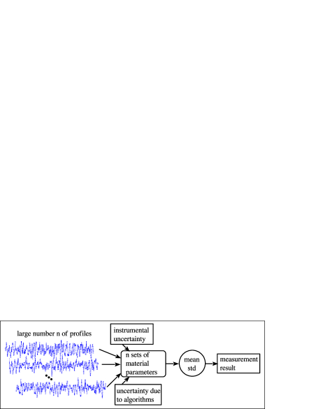
Figure 1: According to the vocabulary of metrology the measurement result requires to state an uncertainty in addition to the physical quantity itself. The uncertainty usually is obtained from sufficient statistics, taken from a large number of profiles on one surface.

For non-deterministic, i.e. stochastic topographies, a major contribution to the uncertainty of roughness parameters besides instrumental limits is its inhomogeneity, the variation of the topography itself. It is the interrelation between bandwidth limit of probing, relocation of samples with size, correlation lengths, periodicities, and randomness of the structures and features of the topography. Therefore performing a Monte Carlo simulation of the instrumental contributions without considering the interactions with the object only gives a component of the error budget that may be significantly smaller than the topography induced contribution. There is a strong demand for modeling the surface topography as well. A sufficiently representative set of profile resp. areal scans of the appropriate bandwidth are required to assess the texture characteristics of a surface. An uncertainty assessment must be made in addition to stating a measured quantity as measurement result in the sence of the international vocabulary of metrology, which states that a measurement result is generally expressed as a measured quantity value and a measurement uncertainty. For the aspect of surface inhomogeneity, a larger number of values for each of the roughness parameters is required. Let $R_{\mathrm{x},i}$ be one of the roughness parameters of profile $i$, then the mean is estimated by $\bar{R}_{\mathrm{x}}=\frac{1}{n}\,\sum_{i=1}^{n}R_{\mathrm{x},i}$ and the standard deviation $s\colon(R_{\mathrm{x},1},\dots,R_{\mathrm{x},n})\,\mapsto\,s(R_{\mathrm{x},1},\dots,R_{\mathrm{x},n})$ by $s(R_{\mathrm{x}})=\sqrt{\frac{1}{n-1}\,\sum_{i=1}^{n}(R_{\mathrm{x},i}\,-\,\bar{R}_{\mathrm{x}})^{2}}$. Then mean and standard deviation of the roughness parameters can be evaluated to obtain a measurement result as illustrated in Fig. 1. Regarding nowadays computer technology and comparing it to instrumentation, it is often the case that simulations are faster and less expensive than measurements. In case of tactile instruments the measurement process may cause wear or even damage. Therefore, Monte Carlo simulations may be preferred, if there exists à priori knowledge of the statistical behavior of the data for deriving simulation results from the data with insufficient empirical statistics. In addition to the statistical analysis of the topography influence, the uncertainties caused by the instrumental devices as well as those caused by the choice of the algorithmic procedures, i.e. the filtration methods [9] and the way of evaluating the Abbott curve, contribute to the final result.

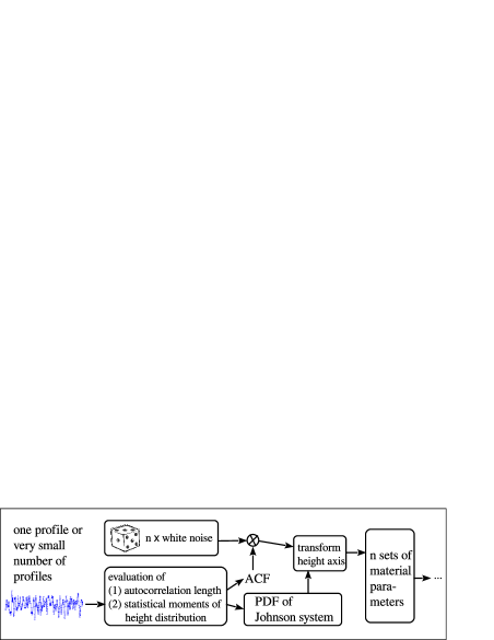
Figure 2: With à priori knowledge of the statistical behavior of the data, the uncertainty could approximately be estimated by deriving simulation results from the data with insufficient statistics.

For more than fourty years a variety of models to describe and simulate the roughness of surface topographies have already been developed employing approaches of random field theory, time series, and non-causal stochastic processes [10]. Wu [11] compares the approaches to convolve white noise with appropriate weight functions that are either obtained by autocorrelation resp. the power spectrum density [12] or by auto regressive (AR) models [13], or the approach to use the power spectrum and instead of multiplying it with the Fourier transform of white noise, to multiply it with uniformly random distributed phases. Uchidate has investigated non-causal AR-models for surface topographies [14], because space is not restricted to causality as time does. A method of obtaining random data while maintaining the correlation properties was given by Theiler et al. [15], which has applied to roughness measurements by Morel [16].

Many of the roughness models presume that surface heights are normally distributed, i.e. that they have a Gaussian shaped amplitude distribution. The deviation from this presumption is quantified by the roughness parameters $R_{\mathrm{sk}}$, which is the skewness, i.e. the third statistical moment, and $R_{\mathrm{ku}}$, which is the kurtosis or excess, i.e. the fourth statistical moment, of the probability density function of topography height values. To parameterize non-Gaussian probability density distributions such that the distributed quantity is transformed to a quantity that then has a Gaussian probability density distribution, a system of functions has been introduced by Johnson in 1949 [17]. To estimate the appropriate function of that set with its parameters accordingly, Hill, Hill, and Holder [17] have developed an algorithm in 1976 that we are employing for our suggested procedure. For more than fifteen years, the Johnson system has been applied to roughness analysis and simulation [18, 19].

Stochastic data require huge samples for statistical analysis and assessment. In quality assurance in industrial life, however, small representative samples are drawn to spot-check a process or pieces. Therefore, we have investigated, how well the uncertainty of material ratio parameters of roughness data can be estimated from a single measurement, one profile or a single area scan. In the next section, the definition according to ISO standards of material ratio parameters will be presented and the ambiguities of the definition will be discussed. Section three deals with the influence of sampling effects on the autocorrelation function ACF and on the probability density function PDF of a topography revealing the sampling effect by looking at synthetic, well defined topographies, defined by Fourier series. In section four, we will give details on the probability density distributions that are useful to describe amplitude distributions of roughness profiles. Section five is dedicated to show a way for an approximate estimation of the inhomogeneity component of the uncertainty of the material ratio parameters by deriving Monte Carlo simulated profiles from a small set of profiles or even a single profile as depicted in Fig. 2. The procedure is a coarse guess being helpful for industrial processes, but does not preempt from taking large data samples to obtain reliable statistical results for research purposes.

The proposed procedure is based on investigations on simulated synthetic profiles of known Fourier series components as well as experimental profiles of a tactile areal profiler, a custom built micro topography measurement system [20]. The vertical axis of the measurement system is realized by a stylus with its vertical movement measured interferometrically directly in line with its probe tip, i.e. without Abbé offset and without any arc error. The stylus is guided by an air pressure bearing and its probing force is controlled by magnetic fields.

The experimental data have been taken on different kind of industrial surfaces. The experiments were carried out on an area of $4\times 4\;\mathrm{mm}^{2}$ on surfaces with $R_{\mathrm{a}}$ values lying in an interval of $(0.1,\,2]\;\mathrm{\mu m}$ according to ISO 4288:1996/Cor 1:1998. The filtration cuts off the waviness contribution by wavelength $\lambda_{\mathrm{c}}$ and the high frequency contribution by wavelength $\lambda_{\mathrm{s}}$ to suppress noise, to reduce apparent low frequencies induced by the folding of frequencies around the sampling frequency [21], and to match instrumental bandwidths [5]. ISO 4288 defines the choice of the cut off wavelengths $\lambda_{s}$ and $\lambda_{c}$ according to the amplitude parameters $R_{\mathrm{a}}$ and $R_{\mathrm{z}}$. ISO 3274 defines the maximum allowed width of sampling intervals according to the cut off wavelengths, for our experimental setting this is $\Delta x\,\leq\,0.5\,\mathrm{\mu m}$ and the radius of the probe tip is $R\,\approx\,2\,\mathrm{\mu m}$. That means that current ISO standards define the choice of the bandwidth according to amplitude parameters rather than correlation length and other horizontal parameters, an issue that will also be discussed in section three.

2 Definition of Material Ratio Parameters

To clearify the relation between the statistical height distribution of a surface and the roughness parameters that are used to characterize surface contact, this section presents the definition of the material ratio parameters in detail. Abbott and Firestone have proposed to describe the area of contact between surfaces by characterizing the area of each surface as the ratio of air to material at any level $c$. The parameter material ratio $Mr$, also called bearing ratio, is a function of height level $c$ [1]. Let $L$ be the length of the total profile, then the sum of the length pieces $l_{i}$ intersecting the asperities at level $c$, i.e. $l_{i}(c)$, delivers $Mr\equiv r_{\mathrm{M}}$

$$r_{\mathrm{M}}(c)\;=\;\frac{1}{L}\,\sum_{i}l_{i}(c)$$ (1)

as illustrated in Fig. 3. As a double letter identifier is inappropriate for maths formulae, we denote the material $r_{\mathrm{M}}$ rather than $Mr$. The inverse of the function material ratio depending on height level, i.e. the distribution $c$ vs. $r_{\mathrm{M}}$, is called Abbott-Firestone distribution, abbreviated Abbott-curve.

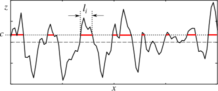
Figure 3: Definition of the material ratio.

The algorithm to evaluate all $l_{i}(c)$ from intersecting asperities and subsequently calculating each intersection between the horizontal line at $z=c$ and the asperities has a complexity that can be avoided if the residual error

$$\Delta r_{\mathrm{M}}(c)\;=\;\sum_{i}\left(\frac{1}{2}\Delta x\,-\,a_{i}\right)$$ (2)

is sufficiently small. The statistical distribution of negative differences $0.5\Delta x\,-\,a_{i}$ is similar to that of positive, so that they almost cancel on average in most cases. The distances $a_{i}$ are those between the intersection of an asperity surface and the neighboring knot of the profile as illustrated in Fig. 4.

A fast and efficient approach is to sort all discrete height values of the equidistantly sampled profile according to their values $z_{i}$

$$z_{i_{1}}\,\geq\,z_{i_{2}}\,\geq\dots\,\geq\,z_{i_{k}}\,\geq\dots\,\geq\,z_{i_{n}}$$ (3)

such that with $L\,=\,(n-1)\,\Delta x$

$$r_{\mathrm{M}}(c=z_{i_{k}})\;\approx\;\frac{\Delta x}{L}\,\sum_{\nu=1}^{k}\left(1\,-\,\frac{1}{2}\delta_{i_{\nu},1}\,-\frac{1}{2}\delta_{i_{\nu},n}\right)$$ (4)

with $(x_{1},z_{1})$ and $(x_{n},z_{n})$ being the border positions of the original profile and $\delta_{i_{\nu},1}$ and $\delta_{i_{\nu},n}$ denoting the Kronecker symbols to treat the border positions appropriately.

Furthermore we approximate this by

$$r_{\mathrm{M}}(c=z_{i_{k}})\;\approx\;\frac{k-0.5}{n}.$$ (5)

Avoiding the values $r_{\mathrm{M}}=0$ and $r_{\mathrm{M}}=1$ is required if the inverse error function $\mathrm{erf^{-1}}$ to parameterize the relation $c$ vs. $r_{\mathrm{M}}$ of profiles with Gaussian distributed height values is used, which is fulfilled by using $k-0.5$ rather than $k$.

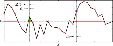
Figure 4: Material ratio with intersections between profile asperities and horizontal line at height level $c$.

The international standard ISO 13565-2 defines a set of $5$ parameters derived from the Abbott-curve for profiles and ISO 25178-2 the corresponding parameters for areal scans:

• the core height $R_{\mathrm{k}}$, which is the distance between the highest and lowest level of the core profile resp. for areal data $S_{\mathrm{k}}$ of the core surface,

• the reduced peak height $R_{\mathrm{pk}}$ and reduced valley/dale height $R_{\mathrm{vk}}$, which are the height of the protruding peaks above the core profile after reduction process in case of $R_{\mathrm{pk}}$ and the height of the protruding dales below the core profile after reduction process in case of $R_{\mathrm{vk}}$. For areal scans they are the height of protruding peaks above resp. dales below the core surface and again the identifier $R$ is replaced by $S$,

• the two material ratio quantities giving once the ratio of the area of the material at the intersection line which separates the protruding hills from the core profile resp. surface to the evaluation area, shortly named peak ratio $\mathrm{Mr}1$ resp. $S_{mr1}$; secondly the ratio of the area of the material at the intersection line which separates the protruding dales from the core profile resp. surface to the evaluation area, shortly named peak ratio $\mathrm{Mr}2$ resp. $S_{mr2}$.

The core height $R_{\mathrm{k}}$ is the negative slope of a regression line within a $40\,\%$ interval for the core material. The $40\,\%$ interval $[r_{\mathrm{M}}(c_{\mathrm{p}}),r_{\mathrm{M}}(c_{\mathrm{v}})]$ with

$$r_{\mathrm{M}}(c_{\mathrm{v}}):=r_{\mathrm{M}}(c_{\mathrm{p}})+0.4$$

is chosen such that the slope of the secant takes a minimum:

$$\min_{c_{\mathrm{p}},c_{\mathrm{v}}}\left\{\frac{c_{\mathrm{p}}\,-\,c_{\mathrm{v}}}{r_{\mathrm{M}}(c_{\mathrm{v}})\,-\,r_{\mathrm{M}}(c_{\mathrm{p}})}\right\}$$ (6)

In case of smooth Abbott-curves this interval coincides well with the interval of minimum slope $R_{\mathrm{k}}$, but not in any case. The search of the minimum secant rather than slope has been chosen at times when computer time was more costly and processing was slow. Furthermore, a discrete set of height values with $c_{\mathrm{v}}$ at a position for $k=\mathrm{v}$, i.e. with $z_{i_{\mathrm{v}}}$ and $c_{\mathrm{p}}=z_{i_{\mathrm{p}}}$ rather than a continous $40\,\%$ interval is used. Consequently the interval is a discretization

$$r_{\mathrm{M}}(z_{i_{\mathrm{v}}})\,-\,r_{\mathrm{M}}(z_{i_{\mathrm{p}}})\approx 0.4$$

approximating $[r_{\mathrm{M}}(c_{\mathrm{p}}),r_{\mathrm{M}}(c_{\mathrm{v}})]$.

If the regression line fitted to the Abbott-curves within $[r_{\mathrm{M}}(c_{\mathrm{p}}),r_{\mathrm{M}}(c_{\mathrm{v}})]$ is given by

$$z(r_{\mathrm{M}})\;=\;-R_{\mathrm{k}}\,r_{\mathrm{M}}\;+\;c_{1},$$ (7)

the parameter $R_{\mathrm{k}}$ is called core height.

For an amplitude distribution of sample size $n\rightarrow\infty$ and if it is a Gaussian, the Abbott curve is the inverse error function $\mathrm{erf}^{-1}$, thus the negative slope at the position $r_{\mathrm{M}}=0.5$ is $\sqrt{2\pi}\,R_{\mathrm{q}}$. The negative of the slope of a regression line to $\mathrm{erf}^{-1}$ for $r_{\mathrm{M}}\in[0.3,0.7]$ is $R_{\mathrm{k}}\cong 2.5739\,R_{\mathrm{q}}$ [22], which is greater than the slope at the $50\%$-position with $\sqrt{2\pi}\cong 2.5066$.

If $c_{2}\,=\,c_{1}\,-\,R_{\mathrm{k}}$ the ratio parameters $\mathrm{Mr}1\equiv r_{1}$ and $\mathrm{Mr}2\equiv r_{2}$ are obtained via the inverse Abbott-curve

$$r_{1}\;=\;r_{\mathrm{M}}(c_{1})\qquad\mathrm{and}\qquad r_{2}\;=\;r_{\mathrm{M}}(c_{2}).$$ (8)

If there exists a positive integral $A_{1}$ of the Abbott-curve above the height level $c_{1}$ within the interval $[0,r_{\mathrm{1}}]$

$$A_{1}\;=\;\int_{0}^{r_{1}}\,(c(r_{\mathrm{M}})-c_{1})\;\mathrm{d}\,r_{\mathrm{M}}\;>\;0$$ (9)

and for the dales a positive integral $A_{2}$

$$A_{2}\;=\;\int_{r_{2}}^{1}\,(c_{2}-c(r_{\mathrm{M}}))\;\mathrm{d}\,r_{\mathrm{M}}\;>\;0$$ (10)

the parameters $R_{\mathrm{pk}}$ and $R_{\mathrm{vk}}$ are defined as

$$R_{\mathrm{pk}}\;=\;\frac{2\,A_{1}}{r_{1}}\qquad\mathrm{and}\qquad R_{\mathrm{vk}}\;=\;\frac{2\,A_{2}}{1-r_{2}}.$$ (11)

Topographies with amplitude distributions of kurtosis values much smaller than 3, for instance sinusoidal grids, have no values above and below the core levels, i.e. no positive values for $A_{1}$ and $A_{2}$ and therefore no reduced peak and dale heights.

We illustrate the effect of the choice of the Abbott-curve algorithm on the values of the material ratio parameters using our measurements on ground steel. One of the profiles of scan length $L=4\,\mathrm{mm}$ and of a correlation length $l_{\mathrm{c}}=6.1\,\mathrm{\mu m}$ being measured with a sampling interval of $\Delta x=0.1\,\mathrm{\mu m}$ is taken exemplarily. The relative difference of the material ratio parameters whether obtained from the Abbott-curve by sorting or by explicit material ratio evaluation lies below $10^{-4}$ if $\Delta x=0.1\,\mathrm{\mu m}$. To reveal the effect, we reduced the resolution artificially by resampling the profile with an interval of $\Delta x=0.5\,\mathrm{\mu m}$. To show the dependence on the raggedness we then evaluated the Abbott-curve of the down sampled profile once without any software cut off of high frequencies, i.e. the lateral limitation purely arises from the finite size of the probing sphere of a tip radius of approximately $2\,\mathrm{\mu m}$. In order to illustrate that the difference between the algorithms reduces the smoother the profile, we simply performed some low pass filtration on the downsampled profile cutting off $\lambda_{\mathrm{s}}=8\,\mathrm{\mu m}$ and furthermore cutting off at a wavelength of $\lambda_{\mathrm{s}}=25\,\mathrm{\mu m}$. Regarding the difference between the $R_{\mathrm{k}}$-value obtained by the sorting method $R_{\mathrm{k,srt}}$ and the $R_{\mathrm{k}}$-value obtained by material ratio calculation $R_{\mathrm{k,mrc}}$ interpolating linearly at the intersection between height levels $c$ and asperity surfaces and the mean between those two values, we evaluate following ratio to get the relative difference.

$$\Delta_{\mathrm{rel}}(R_{\mathrm{k}})\;=\;\frac{R_{\mathrm{k,srt}}\,-\,R_{\mathrm{k,mrc}}}{\frac{1}{2}(R_{\mathrm{k,srt}}\,+\,R_{\mathrm{k,mrc}})}$$ (12)

Evaluating the relative differences for all parameters delivers:

$\lambda_{\mathrm{s}}$/$\mathrm{\mu m}$	-	$8$	$25$
$\Delta_{\mathrm{rel}}(R_{\mathrm{k}})$	$8.7\cdot 10^{-3}$	$1.1\cdot 10^{-3}$	$0.5\cdot 10^{-3}$
$\Delta_{\mathrm{rel}}(R_{\mathrm{pk}})$	$-7.0\cdot 10^{-3}$	$-15.7\cdot 10^{-3}$	$-6.0\cdot 10^{-3}$
$\Delta_{\mathrm{rel}}(R_{\mathrm{vk}})$	$5.6\cdot 10^{-3}$	$5.0\cdot 10^{-3}$	$0.4\cdot 10^{-3}$
$\Delta_{\mathrm{rel}}(r_{1})$	$-8.8\cdot 10^{-3}$	$4.2\cdot 10^{-3}$	$-6.0\cdot 10^{-3}$
$\Delta_{\mathrm{rel}}(r_{2})$	$1.5\cdot 10^{-3}$	$0.2\cdot 10^{-3}$	$<10^{-4}$

The sorting approximation according to Eqn. (3) - (5) delivers the cumulative height distribution of a topography. Therefore, the parameters $R_{\mathrm{k}}$, $R_{\mathrm{pk}}$, and $R_{\mathrm{vk}}$ are directly related to the PDF of the height values. In the next two sections, we will discuss the characteristics of PDFs of surface topographies in detail, first the way how sampling influences its appearance and then we present the classification of PDF types in statistics.

3 Influence of Sampling on ACF and PDF

As topographies of rough surfaces still have regular structures, in particular those originating from machining processes with rotating bodies thus producing periodic cutting traces, uniform sampling may cause aliasing and leakage effects. Therefore, the ratio between sampling interval $\Delta x$ and autocorrelation length $l_{\mathrm{c}}$ on one side and the ratio between sampling length $L$ and autocorrelation length $l_{\mathrm{c}}$ on the other side are the determining quantities for the reliability of the discretization of a topography. Consequently, Bushan suggests to use the correlation length to define the sampling length $L$ [1]. Let $C\colon x\,\mapsto\,C(x)$ be the autocorrelation function

$$C(x)\;=\;\int_{-\infty}^{\infty}z(x)\,z(x-\xi)\,\mathrm{d}\xi$$ (13)

and the autocorrelation length defined to be the length $x_{\mathrm{c}}$ where $C$ takes a certain value $C(x_{\mathrm{c}})\,=\,C_{\mathrm{c}}$. Bushan sets $C_{\mathrm{c}}\,=\,0.1$ denoting it $x_{\mathrm{c}}\,=:\,\beta^{\ast}$, commonly $C_{\mathrm{c}}\,=\,e^{-1}$ as in [12] denoting it $x_{\mathrm{c}}\,=:\,\lambda_{0}$, and in ISO 25178-2 it is $C_{\mathrm{c}}\,=\,0.2$. In this article, we define $x_{\mathrm{c}}\,=:\,l_{\mathrm{c}}$ for $C_{\mathrm{c}}\,=\,0.2$. Bushan’s suggestion of an appropriate profile length of random surfaces to be

$$L\;\geq\;200\,\beta^{\ast}$$ (14)

means that $L$ should be around $300\,l_{\mathrm{c}}$. We have examined a ground steel surface with $300\,l_{\mathrm{c}}\,=\,1.6\dots 2.4\,\mathrm{mm}$ which is about half of the sampling length according to ISO 4288 of $4\,\mathrm{mm}$. We also have examined a ceramics surface of cutting tool inserts with $300\,l_{\mathrm{c}}\,=\,1.8\dots 3.0\,\mathrm{mm}$ and a few outlying profiles, where $300\,l_{\mathrm{c}}$ took values above the $L=4\,\mathrm{mm}$ in the range of $4.3\dots 5.7\,\mathrm{mm}$.

For the sampling interval Bushan suggests $\Delta x\;<\;0.25\,\beta^{\ast}$, i.e. $\Delta x\;<\;0.35\,l_{\mathrm{c}}$, at least $\Delta x\;<\;0.5\,\beta^{\ast}$. In 1989, Ogilvy and Foster [12] have examined the influence of the sampling interval on the shape of the resultant autocorrelation function and its deviation from the original exponential progress. They state that a sampling interval of $\Delta x\;<\;15^{-1}\,\lambda_{0}$ ($\Delta x\;<\;0.04\,l_{\mathrm{c}}$) would be adaequate to detect the exponential nature of the autocorrelation function, which according to them is most likely for rough surface topographies, thus for the surfaces under investigation at around $\Delta x\,=\,0.2\dots 0.3\,\mathrm{\mu m}$. According to ISO standard our surfaces should be sampled with at most $\Delta x\,=\,0.5\,\mathrm{\mu m}$ and we have measured with a sampling interval of $\Delta x\,=\,0.1\,\mathrm{\mu m}$. The suggestions of Bushan originate from the late 1980s and beginning of 1990s, while nowadays instrumental and computational technologies allow broader bandwidths.

Finite and uniform sampling causes an exponential autocorrelation of a rough surface to show ripples like a sinc function or a Bessel function, since they are caused by the convolution with an impulse train of Dirac or box pulses. In order to illustrate the relation between sampling and the shape of the ACF as well as the shape of the PDF, we have generated roughness profiles that we could describe analytically choosing Fourier series of a finite set of spatial frequencies that means of reciprocal wavelengths $\lambda$. Two types of probability density distributions of the frequency sets are compared: a one-sided Gaussian and a uniform distribution. For the one-sided Gaussian we employ

$$\mathcal{N}(\lambda_{\mathrm{m}},\lambda_{\mathrm{BW}})\;\propto\;e^{-\frac{1}{2}\,\left(\frac{\lambda\,-\,\lambda_{\mathrm{m}}}{\lambda_{\mathrm{BW}}}\right)^{2}}\qquad\lambda\,\geq\,\lambda_{\mathrm{m}}$$ (15)

where $\lambda_{\mathrm{BW}}$ denotes the width and $\lambda_{\mathrm{m}}$ denotes the center of the Gaussian distribution and the maximum probability. With $\lambda\,\geq\,\lambda_{\mathrm{m}}$ the parameter $\lambda_{\mathrm{m}}$ denotes the left border of the interval so the smallest wavelength (highest spatial frequency). The diced wavelengths $\lambda$ will scatter close to $\lambda_{\mathrm{m}}$ on the right side, i.e. within an interval of about $[\lambda_{\mathrm{m}},\lambda_{\mathrm{m}}+3\lambda_{\mathrm{BW}}]$. For the uniform distribution we use

$$\mathcal{U}(\lambda_{\mathrm{m}},\lambda_{\mathrm{BW}})\;\propto\;\left\{\begin{array}[]{cl}const.&\lambda\,\in\,[\lambda_{\mathrm{m}},\lambda_{\mathrm{m}}+\lambda_{\mathrm{BW}}]\\ 0&\mathrm{else}\end{array}\right..$$ (16)

where $\lambda_{\mathrm{BW}}$ denotes the width of the scattering interval and $\lambda_{\mathrm{m}}$ the left side of the interval.

Sets of $N$ wavelengths $\{\lambda_{1},\dots,\lambda_{N}\}$ are diced according to the above listed distributions, furthermore $N$ phases $\{\varphi_{1},\dots,\varphi_{N}\}$ are diced according to a uniform distribution with $\varphi_{\nu}\,\in\,[-\pi,\pi]$, and amplitudes $a_{\nu}\,\propto\,\mathrm{exp}(-\lambda_{\nu}/(10^{-3}\,\mathrm{\mu m}))$ were chosen, $\nu=1,\dots,N$. A continuous profile is synthesized for $x$ being the continuous lateral position, i.e. for $x\in\mathrm{I\!R}$

$$z(x)\;=\;\sum_{\nu=1}^{N}a_{\nu}\,\sin\left(\frac{2\,\pi}{\lambda_{\nu}}\,x\;+\;\varphi_{\nu}\right).$$ (17)

For a Dirac pulse sampling the profile is discretized as

$$z(x_{i})\;=\;\sum_{\nu=1}^{N}a_{\nu}\,\sin\left(\frac{2\,\pi}{\lambda_{\nu}}\,(i-1)\,\Delta x\;+\;\varphi_{\nu}\right)$$ (18)

with $i=1,\dots,n$ and for a box pulse train with a pulse width $w$ the profile samples are

$$z(x_{i})\;=\;\sum_{\nu=1}^{N}a_{\nu}\,\int_{A_{i}}^{B_{i}}\sin\left(\frac{2\,\pi}{\lambda_{\nu}}\,\xi\;+\;\varphi_{\nu}\right)\,\mathrm{d}\xi$$ (19)

with

$$A_{i}\;=\;(i-1)\,\Delta x\,-\,\frac{w}{2};\qquad B_{i}\;=\;(i-1)\,\Delta x\,+\,\frac{w}{2}.$$

The origin of ripples of the autocorrelation function $C$ may as well be due to the finite sample size of contributing spatial frequencies $N$. Furthermore, the kind of distribution of the frequencies contributing to the Fourier series determines whether $C$ is better represented by an exponential or by a Gaussian function. Fig. 5 shows the ACFs of two different Fourier series, both with $N=431$ spatial frequencies. The black solid curve is the one obtained from the profile with uniformly distributed spatial wavelengths with $\lambda_{\mathrm{m}}\,=\,11.3\,\mathrm{\mu m}$ and $\lambda_{\mathrm{BW}}\,=\,102\,\mathrm{\mu m}$ delivering a correlation length of $l_{\mathrm{c}}\,=\,11.56\,\mathrm{\mu m}$, which is to be compared to the Gaussian ACF visualized as red dashed curve. The black dash-dotted curve is the ACF obtained from the profile with Gaussian distributed wavelengths with $\lambda_{\mathrm{m}}\,=\,2.6\,\mathrm{\mu m}$ and $\lambda_{\mathrm{BW}}\,=\,53\,\mathrm{\mu m}$ delivering a correlation length of $l_{\mathrm{c}}\,=\,8.6\,\mathrm{\mu m}$, to be compared to the exponential ACF visualized as blue dotted curve and to which we will refer as profile G.

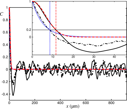
Figure 5: Autocorrelation functions of two different Fourier series: 1. from uniformly distributed spatial wavelengths (black solid curve) with $\lambda_{\mathrm{m}}\,=\,11.3\,\mathrm{\mu m}$ and $\lambda_{\mathrm{BW}}\,=\,102\,\mathrm{\mu m}$, correlation length of $l_{\mathrm{c}}\,=\,11.56\,\mathrm{\mu m}$ and Gaussian ACF (red dashed curve); 2. from Gaussian distributed wavelengths (black dash-dotted curve) with $\lambda_{\mathrm{m}}\,=\,2.6\,\mathrm{\mu m}$ and $\lambda_{\mathrm{BW}}\,=\,53\,\mathrm{\mu m}$, correlation length of $l_{\mathrm{c}}\,=\,8.6\,\mathrm{\mu m}$ and exponential ACF (blue dotted curve).

In Fig. 5 we can see that significant high frequency contributions owe the exponential behavior of the ACF. Be it due to lower resolution as investigated by Ogilvy and Foster or due to the fact that there exist as little high frequencies as low frequencies as we have calculated it here. The resultant ACFs have a Gaussian behavior in both cases. To show the effect of lateral resolution, we have calculated the discretization of profile G for a Dirac impulse train, and box impulse trains with three different widths $w$. Fig. 6 shows the ACF of the data by Dirac impulse train as blue solid curve, those of box impulse trains with $w=0.8\,\mathrm{\mu m}$ as light green dash-dotted curve, $w=2.5\,\mathrm{\mu m}$ as red dashed curve, and $w=5.0\,\mathrm{\mu m}$ as black dotted curve. Since the Fourier series minimum value of wavelength is $\lambda_{\mathrm{m}}=2.6\,\mathrm{\mu m}$, the difference between the box (light green dash-dotted) and the Dirac impulse (blue solid) trains is negligible. In accordance with Ogilvy and Foster the larger the box width, i.e. the smaller the resolution, the more the ACF turns to a Gaussian curve shape.

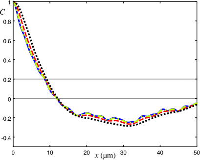
Figure 6: Autocorrelation functions of the Fourier series after being sampled differently: 1. Dirac impulse train (blue solid curve), 2. box impulse train with $w=0.8\,\mathrm{\mu m}$ (light green dash-dotted curve), 3. box impulse train with $w=2.5\,\mathrm{\mu m}$ (red dashed curve), 4. box impulse train with $w=5.0\,\mathrm{\mu m}$ (black dotted curve).

As the ACF it is also the probability density distribution PDF, which is affected by the resolution issue. Fig. 7 shows the PDFs of profile G for three different sampling intervals, with all of them sampled with Dirac pulses. The length of the profile has always been $4\,\mathrm{mm}$ such that the sample size (number of points) $n$ decreases: $\Delta x=0.05\,\mathrm{\mu m}$ with $n=80\,000$ is plotted as solid blue curve, $\Delta x=0.8\,\mathrm{\mu m}$ with $n=5000$ as dotted green curve, and $\Delta x=4\,\mathrm{\mu m}$ with $n=1000$ as dashed red curve.

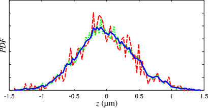
Figure 7: Probability density distribution $\Delta x=0.05\,\mathrm{\mu m}$ solid blue curve, $\Delta x=0.8\,\mathrm{\mu m}$ dotted green, $\Delta x=4\,\mathrm{\mu m}$ dashed red curve.

The PDF is pronged due to the smaller sample size. We have also investigated the effect of the impulse box size on the PDFs for fixed sample sizes. One example for sample size $n=1000$ and different impulse trains is shown in Fig. 8. The blue curve shows the PDF of a profile sampled by a Dirac impulse train, the dashed green curve the PDF with box pulse sampling of width $w=0.8\,\mathrm{\mu m}$, the red dash-dotted curve with $w=2.5\,\mathrm{\mu m}$, and the black dotted curve with $w=5\,\mathrm{\mu m}$.

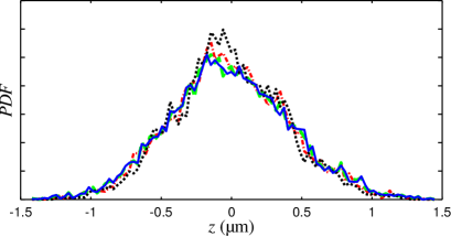
Figure 8: Probability density distribution Dirac solid blue curve, $w=0.8\,\mathrm{\mu m}$ dashed green curve, $w=2.5\,\mathrm{\mu m}$ dash-dotted red, $w=5\,\mathrm{\mu m}$ dotted black curve.

4 PDF Types Parameterizing Roughness Amplitude Distributions

During the past decades, a variety of investigations were made to classify surfaces obtained from different kind of engineering processes according to their amplitude distributions and how they deviate from Gaussian distribution according to their statistical moments and furthermore according to anisotropy and lay.

In 1994, Whitehouse [2] suggested to use different classes of $\beta$-distributions. He derived a relation between the parameters of the $\beta$-distributions and the statistical moments. To describe data that are distributed with long tails generalized extreme value functions are employed, in particular in the field of finance statistics [23]. Extreme value theory has been developed to characterize data with values that extremely deviate from the median of probability distributions [23]. The median is a robust statistical parameter defined to be the middle value of the sorted set of discrete observations of a quantity.

Weibull distributions, as an example of an extreme value distribution, are of particular interest for honed cylinder liner or cylinder running surfaces with oil volume and the elastic-plastic contact of asperities [24].

Since the functions of the Johnson system define non-Gaussian probability density functions that facilitate simulations based on white noise by explicit and invertable transformation $f\colon z\mapsto t(z)$ [25]. We employ Johnson distributions for the Monte Carlo simulation of profiles. They are represented by Gaussian distributions of a transformation of the quantity to be examined, i.e. $\propto exp(-0.5\,t^{2})$. Their relation to statistical moments can be estimated by the Hill et al optimization algorithm of 1976 [17], which is available as Matlab/Gnu-octave routine as well. Johnson defines following three types of transformation functions $f$:

• the lognormal system SL

  $$t\;=\;\gamma\,+\,\delta\,\mathrm{ln}\left(z-\xi\right)\qquad\xi<z$$ (20)

• the unbounded system SU

  $$t\;=\;\gamma\,+\,\delta\,\mathrm{arcsinh}\left(\frac{z-\xi}{\lambda}\right)$$ (21)

• the bounded system SB

  $$t\;=\;\gamma\,+\,\delta\,\mathrm{ln}\left(\frac{z-\xi}{z+\lambda-\xi}\right)\;\;\xi<z<\xi+\lambda$$ (22)

Normally distributed random numbers of a quantity $t$ can then be transformed by using the inverse transformation $f^{-1}\colon t\mapsto z(t)$.

To use the algorithm of Hill et al, we employ the statistics definition of the statistical moments of the PDF, i.e. those with mean subtraction, whereas roughness standards ISO 4287 and ISO 25178-2 define these statistical moments without mean subtraction presuming that the detrending of waviness by cutting off spatial frequencies below $\lambda_{\mathrm{c}}^{-1}$ causes the mean $\bar{z}$ to be very close to zero and hence negligible, i.e.

$$\bar{z}\;=\;\frac{1}{L}\int_{0}^{L}z(x)\mathrm{d}x\;\approx\;0.$$ (23)

The third moment in roughness metrology is

$$R_{\mathrm{sk}}\;=\;\frac{1}{L\,R_{\mathrm{q}}^{3}}\int_{0}^{L}\left(z(x)\right)^{3}\mathrm{d}x$$ (24)

while in statistics and as input for Hill et al we use

$$\mu_{3}\;=\;\frac{1}{n\,s^{3}}\sum_{i=1}^{n}\left(z_{i}-\bar{z}\right)^{3}$$ (25)

with $\bar{z}$ being the mean of all $z_{i}$, called first moment. The fourth moment or kurtosis is

$$R_{\mathrm{ku}}\;=\;\frac{1}{L\,R_{\mathrm{q}}^{4}}\int_{0}^{L}\left(z(x)\right)^{4}\mathrm{d}x$$ (26)

respectively

$$\mu_{4}\;=\;\frac{1}{n\,s^{4}}\sum_{i=1}^{n}\left(z_{i}-\bar{z}\right)^{4}$$ (27)

with the second moment being

$$R_{\mathrm{q}}^{2}\;=\;\frac{1}{L}\int_{0}^{L}\left(z(x)\right)^{2}\mathrm{d}x$$ (28)

respectively the variance, i.e. the square of the standard deviation $s$

$$s^{2}\;=\;\mu_{2}\;=\;\frac{1}{n-1}\sum_{i=1}^{n}\left(z_{i}-\bar{z}\right)^{2}.$$ (29)

and with $x$ being the lateral position, $L$ the length of the profile, $n$ the number of sampling points, and $z$ the roughness profile after band limitation by detrending filtration.

Now we regard our measurement on ground steel with $\Delta x=0.1\,\mathrm{\mu m}$ and $L=4\;\mathrm{mm}$, i.e. with $n=40\,000$ with scanning direction orthogonal to the lay.

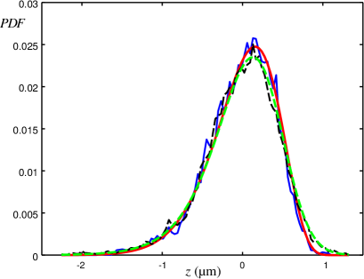
Figure 9: Probability density distributions of 2 scans on a ground steel surface sanned perpendicular to the lay with $\Delta x=0.1\,\mathrm{\mu m}$ and their estimates of Johnson system’s functions: the PDF of the data plotted as black dashed curve is parameterized with a function of the unbounded system (green dashed curve); the PDF plotted as blue solid curve with a function of the bounded system (red solid curve).

Estimation of a PDF of the Johnson system via statistical moments delivered functions of the SU type for some of the profiles and the SB type for most of the profiles. Fig. 9 shows exemplarily two of $1000$ parallel profiles. The two displayed profiles lie $4\;\mathrm{mm}$ appart, one parameterized with a PDF of the SU the other of the SB type. Using the Johnson’s system function (green dashed curve) of the second profile’s PDF plotted as black dashed curve and simulating $20$ profiles according to its autocorrelation length, which has a value of $l_{\mathrm{c}}=6\,\mathrm{\mu m}$, and with $\Delta x=0.4\,\mathrm{\mu m}$ delivers the PDFs shown in Fig. 10.

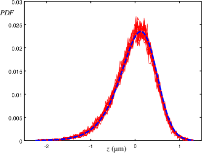
Figure 10: Probability density functions (red solid curves) obtained by simulating $20$ profiles according to its autocorrelation length, which has a value of $l_{\mathrm{c}}=6\,\mathrm{\mu m}$, and with $\Delta x=0.4\,\mathrm{\mu m}$ using the Johnson’s system function (blue dashed curve).

The ceramics sample that we have investigated shows extremely deep pores such that the PDFs have a significant long left tail biasing the statistical moments. To obtain statistical moments delivering appropriate Johnson system functions, we have eliminated the height values below $-2.5\,\mathrm{\mu m}$ when evaluating the statistical moments. Fig. 11 shows the PDFs of two of the measured profiles together with the estimated SU functions for each of them.

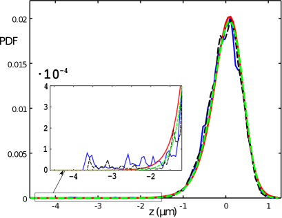
Figure 11: Probability density distribution of 2 example scans on a ceramics surface. The measurment plotted as solid blue curve has been parameterized with a Johnson’s SU function, which is drawn as solid red curve; the measurment drawn as dashed black curve estimated with that of dashed green curve. Moment estimations required a cut off of values $z\leq-2.5\,\mathrm{\mu m}$ to deal with the extraoridinarily long tails to reproduce the shape of the core of the PDFs.

The requirement of tail elimination for the scans on the ceramics surface shows the limits of the procedure to employ statistical moments for a subsequent estimation of Johnson system’s functions. For a more intricate investigation, hence more complex Monte Carlo approaches, a mixing of more than one stochastic process is needed. A mixing may be achieved by superimposing profiles and finally PDFs. Typical examples for such superpositions are surfaces obtained by different steps of machining processes such as honing after grinding. The grinding delivers deep grooves and dales, for instance as oil volume, and the honing smoothes the upper part of the surface to decrease friction. Pawlus superimposes two Gaussian distributed surfaces to simulate this type of surfaces [26]. This approach will be investigated more thoroughly with regard to the statistics of topographies produced by different machining steps. We are considering a combination of Gaussian and non-Gaussian PDFs for future work [27]. A generalized approach of a superpositioning of Gaussian processes is the Gaussian mixture density modeling, which has already been investigated twenty years ago [28].

5 Approximating Material Ratio Uncertainties

In this section, we now present a procedure for estimating the uncertainty contribution to roughness parameters caused by the stochasticity of the topography of the measured surface. In order to investigate its possibilities and limitations we have examined surfaces of different material and different type of machining, topographies with lay and isotropical textures. All surfaces under investigation for this article have $R_{\mathrm{k}}$ values in the order of magnitude of $1\;\mathrm{\mu m}$. They show standard deviations of $R_{\mathrm{k}}$ that lie in the range of two to five percent. The standard deviation of $R_{\mathrm{pk}}$ and that of $R_{\mathrm{vk}}$ are in the same order of magnitude than that of $R_{\mathrm{k}}$ in their absolute values, such that their relative deviation is greater accordingly. To demonstrate our Monte Carlo approach with its advantages and drawbacks here, we have chosen the profiles measured on our ground steel sample.

The proposed procedure only provides for an approximate estimate of the uncertainty of material ratio parameters. It does not replace the characterization of the texture over a macroscopic range. The method procedes as follows:

1. numerical evaluation of ACF of the discrete profile of $n$ height values $\{z_{1},\dots,z_{n}\}$ with calculation of the autocorrelation length $l_{\mathrm{c}}$ by selecting the first intersection of the ACF curve with $C=0.2$;

2. choose the appropriate model for ACF, either exponential or Gaussian, then evaluate $C(x,l_{\mathrm{c}})$ and its power spectrum density for a discrete sample of sample size $n$; use Fourier transform of weights $\{w_{1},\dots,w_{n}\}$ that are derived from $C(x_{i},l_{\mathrm{c}})$ according to [12];

3. estimate the statistical moments of the profile $\{z_{1},\dots,z_{n}\}$ according to Eqn. (23), (25), (27), and (29) and estimate function of Johnson system;

4. perform $K$ times (for instance $K=100$), i.e. $\kappa=1,\dots,K$ the following sub-steps:

   1. generate random white noise $\{r_{1},\dots,r_{n}\}_{\kappa}$ of sample size $n$ and convolve it with the weights $\{w_{1},\dots,w_{n}\}$ such that a correlated sequence of values $\{t_{1},\dots,t_{n}\}_{\kappa}$

      $$t_{i}=\sum_{\nu}w_{\nu}r_{i+\nu}$$ (30)

      is obtained with $w_{\nu}$ such that

      $$C(x_{i},l_{\mathrm{c}})=\sum_{\nu}t_{\nu}t_{i+\nu}$$ (31)

      by multiplication in Fourier space accordingly;

   2. transform sequence $\{t_{1},\dots,t_{n}\}_{\kappa}$ via inverse function $f^{-1}$ of Johnson system’s function to obtain a simulated profile $\{{\tilde{z}}_{1},\dots,{\tilde{z}}_{n}\}_{\kappa}$

   3. evaluate the set of material ratio parameters $R_{\mathrm{k},\kappa}$, $R_{\mathrm{pk},\kappa}$, etc. of the simulated profile $\{{\tilde{z}}_{1},\dots,{\tilde{z}}_{n}\}_{\kappa}$

5. evaluate mean and standard deviation of each of the material parameters over $K$ values:

   $$\bar{R}_{\mathrm{k}}\;=\;\frac{1}{K}\sum_{\kappa=1}^{K}R_{\mathrm{k},\kappa}\qquad\mathrm{etc.}$$

   and

   $$s(R_{\mathrm{k}})\;=\;\sqrt{\frac{1}{K-1}\sum_{\kappa=1}^{K}\left(R_{\mathrm{k},\kappa}\,-\,\bar{R}_{\mathrm{k}}\right)^{2}}\qquad\mathrm{etc.}$$

On ground steel, we have measured $1000$ profiles with a sampling interval of $\Delta x=0.1\,\mathrm{\mu m}$. The mean observed autocorrelation length is $l_{\mathrm{c}}=6\,\mathrm{\mu m}$. The covered area takes $4\,\times\,4\,\mathrm{mm}^{2}$. We have observed significantly varying $R_{\mathrm{q}}$ values as well as varying skewness and kurtosis as can be seen in Fig. 12 as blue circles.

Empirical result of $1000$ measured profiles
	$R_{\mathrm{k}}$	$R_{\mathrm{pk}}$	$R_{\mathrm{vk}}$	Mr1	Mr2
	$\mathrm{\mu m}$	$\mathrm{\mu m}$	$\mathrm{\mu m}$	%	%
mean	1.07	0.27	0.64	7.2	86.3
$s$	0.04	0.05	0.04	0.8	0.9

The standard deviations $s$ of $R_{\mathrm{k}}$, $R_{\mathrm{pk}}$, and $R_{\mathrm{vk}}$ have values of around $50$ Nanometer. To compare the experimental result with our Monte Carlo method, we have run the Monte Carlo simulation $20$ times with $100$ profiles each, with $L=4\,\mathrm{mm}$ and $l_{\mathrm{c}}=6\,\mathrm{\mu m}$. To show the influence of resolution we have done this for three different sampling intervals $\Delta x=0.1\,\mathrm{\mu m}$, $\Delta x=0.5\,\mathrm{\mu m}$, and $\Delta x=1\,\mathrm{\mu m}$, delivering following values for the standard deviation of each of the material ratio parameters:

Influence of resolution:
Standard dev. of $20$ simulations of $100$ profiles
$\Delta x$/$\mathrm{\mu m}$	$0.1$	$0.5$	$1$
$s(R_{\mathrm{k}})$/$\mathrm{nm}$	$23\pm 2$	$25\pm 2$	$28\pm 2$
$s(R_{\mathrm{pk}})$/$\mathrm{nm}$	$15\pm 1$	$16\pm 1$	$17\pm 2$
$s(R_{\mathrm{vk}})$/$\mathrm{nm}$	$30\pm 2$	$30\pm 2$	$32\pm 2$
$s$(Mr1)/ %	$0.48\pm 0.03$	$0.53\pm 0.03$	$0.60\pm 0.05$
$s$(Mr2)/ %	$0.69\pm 0.06$	$0.74\pm 0.06$	$0.78\pm 0.06$

The values given in the above table show that the uncertainty of the core height lies around three percent, the uncertainty of the reduced peak and dale heights around six percent.

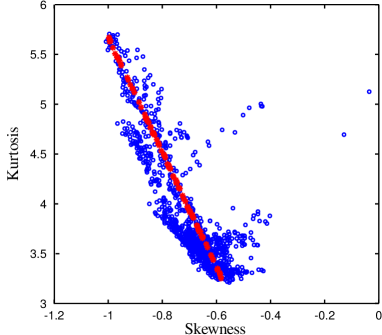
Figure 12: Relation between skewness and kurtosis for a ground steel surface, the blue circles are obtained by experiment and the red asterix are values used for Monte Carlo simulation to be passed to the Johnson system of PDFs.

Similar to the distribution of skewness and kurtosis of the experimental data we have randomly changed the moments for the Johnson functions within the Monte Carlo loop (included step (iii) into step (iv)). Here, we show one example with which we mimic the experimental relation of skewness and kurtosis of the ground surface shown in Fig. 12 as blue circles. We have varied the skewness $\mu_{3}$ due to a uniform distribution then evaluated the kurtosis $\mu_{4}$ to be close to following straight line segment:

$$\left(\begin{array}[]{c}\mu_{3}\\ \mu_{4}\end{array}\right)\in\left[\left(\begin{array}[]{c}-1.0\\ 5.67\end{array}\right),\,\left(\begin{array}[]{c}-0.58\\ 3.25\end{array}\right)\right]$$

The kurtosis has been normally distributed around that line with $\sigma_{\mu_{4}}=0.01$. The diced pairs of $(\mu_{3},\mu_{4})$ are displayed in Fig. 12 as red asterixes. For the sampling interval a value of $\Delta x=0.1\,\mathrm{\mu m}$ has been chosen.

Monte Carlo with varied
skewness and kurtosis
$s(R_{\mathrm{k}})$ / $\mathrm{nm}$	$48\pm 3$
$s(R_{\mathrm{pk}})$ / $\mathrm{nm}$	$27\pm 2$
$s(R_{\mathrm{vk}})$ / $\mathrm{nm}$	$50\pm 4$
$s$(Mr1) / %	$0.56\pm 0.04$
$s$(Mr2) / %	$0.80\pm 0.06$

With a variation of the statistical moments we could take influence on the resulting standard deviation pushing it up to the values of the experimental result revealing that for any engineering process a texture assessment on a prototype is required. For fixed third and fourth moment, just varying the second, the uncertainty of $R_{\mathrm{k}}$ shows the linear relation to that of $R_{\mathrm{q}}$, since they are directly related as the Abbott curve is the cumulative PDF. $s(R_{\mathrm{pk}})$ and $s(R_{\mathrm{vk}})$ are strongly influenced by the higher moments.

In contrast to experiment, the value of the $s(R_{\mathrm{pk}})$ remains smaller while $s(R_{\mathrm{vk}})$ is reproduced well, revealing that the Johnson functions represent the left tail well enough but not the right side of the PDF. This shows that the proposed method gives an approximate estimate, but that a detailed analysis and a precise uncertainty estimate requires a more complex model of the stochastic processes.

6 Conclusion

Deriving the standard deviation of material ratio parameters caused by the inhomogeneity of surface textures can be approximated coarsely from a single scan. A Monte Carlo method that employs the autocorrelation length of the scanned profile and the first four statistical moments of its amplitude distribution has been proposed. It is based on a model autocorrelation function, an exponential or Gaussian, parameterized by the experimental autocorrelation length and on a model probability density function of the Johnson system of which the parameterization is derived from the experimental statistical moments.

Employing only one single profile has the advantage that the procedure can well be implemented into roughness analysis software without any additional statistics information. Our investigations comparing Monte Carlo with a high statistics experiment have shown that this may underestimate the value of the standard deviation. To assess the uncertainty more precisely, more statistics is required, which can well be obtained by scanning more profiles that are irregularly distributed across the surface delivering a greater variation of the Monte Carlo generated profiles. A future goal is to develop more complex but still feasible model of surface texture statistics and a learning system filling a data base for different classes of topographies.
 

We are grateful to the anonymous referees to having taken their time for thoroughly reviewing this article.

References

- [1] Bharat Bhushan. Modern Tribology Handbook, volume 1, chapter 2 Surface Roughness Analysis and Measurement Techniques. CRC Press, 2001. doi:10.1201/9780849377877.ch2.
- [2] David J Whitehouse. Handbook of Surface Metrolotgy, chapter 2 Surface Characterization. IOP Publishing, 1994.
- [3] H. Haitjema. Uncertainty estimation of 2.5-D roughness parameters obtained by mechanical probing. Int. J. Precision Technology, 3(4):403–412, 2013. doi:10.1504/IJPTECH.2013.058260.
- [4] H. Haitjema. Uncertainty in measurement of surface topography. Surf. Topogr.: Metrol. Prop., 3(035004), 2015. doi:doi:10.1088/2051-672X/3/3/035004.
- [5] R. Leach and H. Haitjema. Bandwidth characteristics and comparisons of surface texture measuring instruments. Meas. Sci. Technol., 21:9pp, 2010. doi:10.1088/0957-0233/21/3/032001.
- [6] H. Haitjema and M. Morel. The concept of a virtual roughness tester. Proceedings X. International Colloquium on Surfaces, pages 239–244, 31 Jan - 2 Feb 2000.
- [7] M. Xu, T. Dziomba, and L. Koenders. Modelling and simulating scanning force microscopes for estimating measurement uncertainty: a virtual scanning force microscope. Meas. Sci. Technol., 22:094004 (10pp), 2011. doi:10.1088/0957-0233/22/9/094004.
- [8] C.L. Giusca, R.K. Leach, and A.B. Forbes. A virtual machine-based uncertainty evaluation for a traceable areal surface texture measuring instrument. Measurement, 44:988–993, 2011. doi:10.1016/j.measurement.2011.02.011.
- [9] D. Hüser, P. Thomsen-Schmidt, and R. Meeß. Uncertainty of cutting edge roughness estimation depending on waviness filtration. In Elsevier, editor, 3rd CIRP Conference on Surface Integrity (CIRP CSI), Procedia CIRP, page 4pp, 2016. doi:10.1016/j.procir.2016.02.050.
- [10] T.H. Wu and E.M. Ali. Statistical representation of joint roughness. Int. J. Rock Mech. Min. Sci. & Geomech. Abstr., 15(5):259–262, 1978. doi:10.1016/0148-9062(78)90958-0.
- [11] J.J. Wu. Simulation of rough surfaces with fft. Tribology International, 33:47–58, 2000.
- [12] J.A. Ogilvy and J.R. Foster. Rough surfaces: gaussian or exponential statistics? J. Phys. D: Appl. Phys., 22:1243–1251, 1989.
- [13] Jörg Seewig. Praxisgerechte Signalverarbeitung zur Trennung der Gestaltabweichungen technischer Oberflächen, chapter 5.3 Modell der Rauheit. Shaker, 2000.
- [14] M. Uchidate, T. Shimizu, A. Iwabuchi, and K. Yanagi. Generation of reference data of 3d surface texture using the non-causal 2d ar model. Wear, 257:1288–1295, 2004. doi:10.1016/j.wear.2004.05.019.
- [15] J. Theiler, S. Eubank, A. Longtin, B. Galdrikian, and J. D. Farmer. Testing for non-linearity in time series: the method of surrogate data. Physica D, 58:77–94, 1992.
- [16] Michel A. A. Morel. Uncertainty Estimation of Shape and Roughness Measurement. Diss., Technische Universiteit Eindhoven, 2006.
- [17] I. D. Hill, R. Hill, and R. L. Holder. Algorithm as 99: Fitting johnson curves by moments. J R STAT SOC C-APPL, 25(2):180–189, 1976. doi:10.1007/s10614-006-9025-7.
- [18] S K Chilamakuri and B Bhushan. Contact analysis of non-gaussian random surfaces. Proc. Instn. Mech. Engrs, Part J: J. Eng. Trib., 212:19–32, 1998.
- [19] V. Bakolas. Numerical generation of arbitrarily oriented non-gaussian three-dimensional rough surfaces. Wear, 254:546–554, 2003. doi:10.1016/S0043-1648(03)00133-9.
- [20] P. Thomsen-Schmidt. Characterization of a traceable profiler instrument for areal roughness measurement. Meas. Sci. Technol., 22:11pp, 2011. doi:10.1088/0957-0233/22/9/094019.
- [21] David J Whitehouse. Handbook of Surface Metrolotgy, chapter 3 Processing. IOP Publishing, 1994.
- [22] J. Seewig. The uncertainty of roughness parameters. In AMA, editor, AMA Conferences 2013, Proceedings SENSOR 2013, pages 291–296, 2013. doi:10.5162/sensor2013/B6.2.
- [23] M. Killi and E. Këllezi. An application of extreme value theory for measuring financial risk. Computational Economics, 27(2):207–228, 2006. doi:10.1007/s10614-006-9025-7.
- [24] N. Yu and A.A. Polycarpou. Contact of rough surfaces with asymmetric distribution of asperity heights. J. Tribol, 124:367–376, 2002. doi:10.1115/1.1403458.
- [25] N. L. Johnson. Systems of frequency curves generated by methods of translation. Biometrika, 36(1/2):149–176, 1949. doi:10.2307/2332539.
- [26] P. Pawlus. Simulation of stratified surface topographies. Wear, 264:457–463, 2008. doi:10.1016/j.wear.2006.08.048.
- [27] Sebastian Rief. Dissertation. University of Kaiserlautern, Germany, to be published.
- [28] X. Zhuang and Y. Huang. Gaussian mixture density modeling, decomposition, and applications. IEEE Trans. Image Processing, 5(9):1293–1302, 1996.