Measurements of the Soft Gamma-ray Emission from SN2014J with Suzaku

Abstract

The hard X-ray detector (HXD) onboard Suzaku measured soft $\gamma$-rays from the Type Ia supernova SN2014J at $77\pm 2$ days after the explosion. Although the confidence level of the signal is about 90% (i.e., $2\sigma$), the $3\sigma$ upper limit has been derived at $<2.2\times 10^{-4}$ ph s^-1 cm^-2 in the 170 – 250 keV band as the first independent measurement of soft $\gamma$-rays with an instrument other than INTEGRAL. For this analysis, we have examined the reproducibility of the NXB model of HXD/GSO using blank sky data. We find that the residual count rate in the 90 – 500 keV band is distributed around an average of 0.19% with a standard deviation of 0.42% relative to the NXB rate. The averaged residual signals are consistent with that expected from the cosmic X-ray background. The flux of SN2014J derived from Suzaku measurements taken in one snapshot at $t=77\pm 2$ days after the explosion is consistent with the INTEGRAL values averaged over the period between $t=$50 and 100 days and also with explosion models of single or double degenerate scenarios. Being sensitive to the total ejecta mass surrounding the radioactive material, the ratio between continuum and line flux in the soft gamma-ray regime might distinguish different progenitor models. The Suzaku data have been examined with this relation at $t=77\pm 2$ days, but could not distinguish models between single and double degenerate-progenitors. We disfavor explosion models with larger ⁵⁶Ni masses than 1 $M_{\odot}$, from our $1\sigma$ error on the 170-250 keV X-ray flux of $(1.2\pm 0.7)\times 10^{-4}$ ph s^-1 cm^-2.

1 Introduction

Type Ia supernovae (SNe) are very bright stellar explosions which are detectable at optical wavelengths across cosmological distances. It is widely accepted that they originate from thermonuclear explosions of carbon-oxygen white dwarfs (WDs) in binary systems. They are among the most matured standardizable candles (Phillips et al., 1993; Riess et al., 1998; Perlmutter et al., 1999), having a tight but phenomenologically calibrated relation between the optical peak luminosity and the decline rate of the light curve in the $B$-band.

Table 1: Suzaku Observations towards M82

OBSID	Target Name	Date	HXD Exposure	PIN Count rate	GSO Count rate
		(yyyy/mm/dd)	(ks)	($10^{-2}$ c/s)	($10^{-1}$ c/s)
100033010	M82-Wind	2005/10/04	28.6	$1.6\pm 0.4$	$1.2\pm 1.2$
100033020	M82-Wind	2005/10/19	36.1	$2.6\pm 0.4$	$0.0\pm 1.1$
100033030	M82-Wind	2005/10/28	24.0	$3.2\pm 0.5$	$0.2\pm 0.4$
702026010	M82 X-1	2007/09/24	28.4	$2.6\pm 0.4$	$0.0\pm 0.4$
908005010	SN 2014J	2014/03/30	193.9	$2.6\pm 0.1$	$1.8\pm 0.1$

However, the progenitors of Type Ia SNe have been poorly constrained observationally despite many on-going attempts (see e.g., Maoz, Mannucci, and Nelemans, 2014, for reviews). There are several variants in terms of the ignition and propagation of the thermonuclear flame (Hillebrandt & Niemeyer, 2000), which can have different characteristics in (1) the evolution toward the explosion, and (2) in the mass of the exploding WD. The evolution scenarios are roughly divided into two categories referring to the nature of the progenitor systems; the single degenerate scenario (hereafter SD; Whelan & Iben, 1973; Nomoto, 1982) (a C+O WD and a main-sequence/red-giant companion) or double degenerate scenario (hereafter DD; Iben & Tutukov, 1984; Webbink, 1984) (a merger of two C+O WDs). The mass of the exploding WD(s) is linked to the progenitor systems and their evolution scenario, which would affects on the cosmological usage of SN Ia as distance indicators. In the SD scenario the most popular model involves a Chandrasekhar-mass WD (e.g., Nomoto, 1982). The original DD scenario is also associated with the Chandrasekhar-mass WD (e.g., Iben & Tutukov, 1984). In a recently proposed variant of the DD model, the so-called violent merger model (Pakmor et al., 2010; Röpke et al., 2012), the total mass of the ejecta (i.e., a sum of the two WDs) can exceed the Chandrasekhar-mass limit, a specific model of which is for example presented in Summa et al. (2013). Determining the ejecta mass and/or the progenitor WD is therefore of particular importance (e.g., Scalzo et al., 2014; Yamaguchi et al., 2015; Katsuda et al., 2015).

As demonstrated in the optical light curves of SNe Ia, they produce a large amount of ⁵⁶Ni in the explosion, on average $\sim 0.6M_{\odot}$. Direct measurements of $\gamma$-ray emission from the decay chain, ⁵⁶Ni $\rightarrow^{56}$Co $\rightarrow^{56}$Fe (Arnett, 1979), have been suggested to provide not only the direct evidence for the thermonuclear nature of SNe Ia (Ambwani & Sutherland, 1988; Milne et al., 2004) but also various diagnostics to discriminate different models (e.g., see Maeda et al., 2012; Summa et al., 2013, for predictions based on multi-dimensional explosion models). Among various possibilities, it has been suggested to be a strong probe to the mass of the explosion systems (Sim & Mazzali, 2008; Summa et al., 2013), i.e., either a single Chandrasekhar-mass WD or merging two WDs for which the total mass can exceed the Chandrasekhar-mass.

Despite the strong motivation to analyze the $\gamma$-ray emission from SNe Ia, no solid detection had been reported until 2014, including attempts for SN1991T (Lichti et al., 1994; Leising et al., 1995), SN1998bu (Georgii et al., 2002) and SN2011fe (Isern et al., 2013). The situation changed in 2014, after SN2014J was discovered on 22 January 2014 (Fossey et al., 2014) in the nearby star-burst galaxy M82 at the distance $d\sim 3.5$ Mpc (Dalcanton et al., 2009; Karachentsev & Kashibadze, 2006) and was classified as the closest Type Ia SN (Ayani, 2014; Cao et al., 2014; Itoh et al., 2014) in the last three decades. The reconstructed date of the explosion was 14.75 January 2014 (Zheng et al., 2014). In the MeV $\gamma$-ray band, the INTEGRAL satellite made possible the first detection of ⁵⁶Co $\rightarrow^{56}$Fe lines at 847 and 1238 keV at $(2.34\pm 0.74)\times 10^{-4}$ ph cm^-2 s^-1 and $(2.78\pm 0.74)\times 10^{-5}$ ph cm^-2 s^-1, respectively, in an average of the 50 to 100 days after the explosion (Churazov et al., 2014; Diehl et al., 2015). Even at earlier phases of 20 days after the explosion, the detection of ⁵⁶ Ni $\rightarrow^{56}$Co lines at 152 and 812 keV at $(1.10\pm 0.42)\times 10^{-4}$ ph cm^-2 s^-1 and $(1.90\pm 0.66)\times 10^{-5}$ ph cm^-2 s^-1, respectively, was reported (Diehl et al., 2014). Analysing the time evolution of ⁵⁶Co lines (Diehl et al., 2015; Siegert & Diehl, 2015), a ⁵⁶Ni mass of 0.5 $M_{\odot}$ was derived. But a clear discrimination of models between SD and DD does not seem to be possible, both from limitations of the measured $\gamma$-ray intensity evolution and the theoretical prediction from different models.

These studies provided the first detection of nuclear $\gamma$-ray emission from SNe Ia, and indeed the only detection of nuclear $\gamma$-ray emission from objects beyond the local group of galaxies. This detection relies on the SPI and IBIS instruments on the same satellite INTEGRAL, and additional confirmation by a fully independent instrument is important. Moreover, while these previous reports mostly focused on the detection of the lines, a wealth of additional information is contained in the continuum emission. The MeV decay lines are scattered down to lower energy by Compton scattering, creating continuum emission above $\sim 100$ keV (e.g., Ambwani & Sutherland, 1988; Sim & Mazzali, 2008; Summa et al., 2013). This process is more important for more dense ejecta, unlike the line strengths which become weaker for more dense ejecta. Therefore, combining the information from the lines and the continuum, one expects to obtain additional insight into the properties of the SN ejecta that is then linked to the progenitor star. Indeed, the detection of continuum in the energy range of $200-400$ keV by INTEGRAL was reported by Churazov et al. (2014). In this paper, we report a measurement of the $\gamma$-ray continuum from SN 2014J with the Suzaku X-ray satellite (Mitsuda et al., 2007). In sections 2 and 3 and we test several explosion models to constrain the mass of ⁵⁶Ni and the mass of the exploding WD system in section 4.

2 Observation and Data Reduction

2.1 ToO Observation with Suzaku

The X-ray satellite Suzaku carries two active X-ray instruments onboard (Mitsuda et al., 2007); the X-ray Imaging Spectrometer (XIS; Koyama et al., 2007) and the hard X-ray detector (HXD; Takahashi et al., 2007) to observe the 0.2 – 12 keV and the 13 – 600 keV bands, respectively. The HXD is a hybrid detector with PIN-type Si photo-diodes for the 13 – 70 keV band and phoswitch-type scintillation counters using Gd₂SiO₅ (hereafter GSO) crystals surrounded by Bi₄Ge₃O₁₂ (hereafter BGO) crystals for the 60 – 600 keV band (Takahashi et al., 2007). It has a comparable or better sensitivity than that of INTEGRAL instruments in the 60 – 200 keV band on an ’one-shot’ short observation and therefore, it is suitable for our purpose to independently detect the soft $\gamma$-ray emission from SN2014J.

We triggered ToO observation of SN2014J with Suzaku from 2014 March 30 12:18 UT to 3 April 17:23 UT (OBSID=908005010), which is about $t=77\pm 2$ days after the explosion of SN2014J, soon after the day when the sun angle allows the satellite operation. The target position was set to ($\alpha,\delta$)[J2000] = ($09^{\rm h}55^{\rm m}42.12^{\rm s}$, $+69^{\circ}40^{\prime}26.0^{"}$) at the XIS nominal pointing position. The HXD was operated in the nominal mode; the bias voltages for one half of 64 PIN diodes were operated at 400 V and the other half at 500 V, and the photo-multipliers for scintillators were operated in the nominal setting of the high voltages. We also used previous observations towards the M82 region before the explosion of SN2014J for comparison in later sections. The observation in 2014J with OBSID=908005010 (hereafter OBS2014) and previous ones are summarized in Table 1.

Table 2: Systematic error of HXD-GSO NXB model for OBS2014

ID	Energy band (keV)	Reproducibility (%)
i	86 - 120	0.48
ii	120 - 144	0.55
iii	144 - 176	2.37
iv	176 - 202	0.01
v	202 - 256	0.05
vi	256 - 342	0.55
vii	342 - 500	1.80

2.2 Data Reduction

The observation data-sets were processed by the standard Suzaku pipeline version 2.8.20.35, with the calibration version (CALDBVER) of hxd20110913, xis20121106, xrt20110630, and xrs20060410 for OBS2014. In the analysis of other OBSIDs in the following Section 3, all the data are reprocessed by the ftool, ’aepipeline’, with the latest CALDB files with equivalent version of OBS2014. Spectral fitting was performed with XSPEC version 12.8.1g in HEADAS 6.15.1 package. Background was estimated from models for instrumental (i.e., ’non-X-ray’) background plus cosmic diffuse X-ray background, both fitted to the SN2014J and other independent data (see below).

We did not use the XIS data, because bright X-rays from the ultra-luminous source M82 X-1 strongly contaminated the SN2014J region.

Cleaned event lists of the HXD are obtained by the standard selection criteria. The net exposure for the HXD is 193.9 ks. The non-X-ray background (NXB) is estimated using the methods described in Fukazawa et al. (2009). We used the NXB events of both PIN and GSO with METHOD=”LCFITDT (bgd_d)” and the version of METHODV=2.6ver1110-64. Here, if we subtract NXB events from OBS2014 data, the net count rates of PIN and GSO are $(2.6\pm 0.1)\times 10^{-1}$ c s^-1 and $(1.8\pm 0.1)\times 10^{-2}$ c s^-1, respectively, in the 13 – 70 or the 90 – 500 keV bands, respectively. Count rates for other observations towards M82 than OBS2014 are also summarized in Table 1.

On the HXD PIN detector, the count rate of OBS2014 in Table 1 shows no significant excess over the others. According to Miyawaki et al. (2009), most of PIN signals can be considered as hard X-rays from the ULX M82 X-1, whereas $\gamma$-rays from Type Ia SNe should be weak in this energy band below 100 keV (Maeda et al., 2012; The & Burrows, 2014). Therefore, in the following sections, we concentrate on checking the detectability of $\gamma$-rays from SN2014J with the HXD GSO in the energy band above 90 keV.

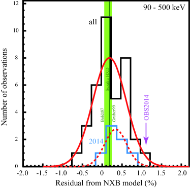
Figure 1: Distributions of residuals of GSO signals of blank sky observations (Table 3) from the NXB models in the 90 – 500 keV band are shown in the histograms. Distribution for all the 37 observations is shown in black and that for 7 selected observations taken within 2 months before or after the SN2014J observation (i.e., OBSIDs in Table3 with note $e$) are in cyan. The best-fit Gaussian models for them are plotted in red. For comparison, the average value for all the blank sky observations (whose spectrum is shown in Figure 5 blue) is shown in dark green line, and the CXB levels by HEAO-1 (Boldt, 1987; Gruber, 1999) are shown in the green hatched box. The residual from the NXB model for OBS2014 is shown in the purple with arrow.

3 Analysis and Results

3.1 Signal Level compared with the Systematics of Non X-ray background

The systematic error is mainly determined by the reproducibility of the NXB model, which is about 1 % or less for GSO in more than 10 ks exposure (Fukazawa et al., 2009). For OBS2014, it was confirmed with the earth occultation data during the observation, whose exposure is only 17.7 ks with standard criteria of Cut-off-Rigidity or 21.5 ks when we do not exclude data with bad conditions of Cut-off-Rigidity (see Table 2). We estimated a systematic uncertainties of 0.1 – 0.6 % (except for one energy bins (iii) and (vii) in the table). Note that the definition of energy bins in Table 2 is determined by bins in the NXB estimation by Fukazawa et al. (2009). In order to perform a more precise check on the reproducibility of the GSO NXB models for longer exposures than 21.5 ks during the sky observations (i.e., not earth occultation data), we estimated them with the “blank sky” observations for the HXD GSO. Among all the Suzaku observations after the launch in 2005 to 2014, we first picked up 140 observations whose exposures of the XIS exceed 120 ks, and then selected “blank sky” observations for GSO with the following criteria: (1) PIN counts in the 50 – 60 keV or the 60 – 70 keV bands do not exceed 3.5% of the NXB models, (2) GSO counts in the 90 – 500 keV do not exceed 2.0% of the NXB models, or the number of energy bands in which GSO counts exceed 1.0% of each NXB level is less than half (i.e., 3 among 7 bands defined in Table 2), (3) the systematic errors of GSO NXB models estimated by the earth data do not exceed 2 %. Finally, we got 37 “blank sky” observations as listed in Table 3. The total exposure of them is 4.49 Ms. The reproducibility of the GSO NXB model for each observation is also listed in the table. As a result, the reproducibility of NXB models distributes in $0.19\pm 0.42$ % for all the 37 observations or $0.34\pm 0.28$ % for observations near the SN2014J date, with $1\sigma$ errors, as demonstrated in Figure 1. Note that this discrepancy (i.e., 0.19% offset here) between blank sky observation and NXB models comes from a contamination of CXB emission in the field of view of the HXD GSO and from the Earth’s albedo emission included in NXB models; the effect is seen in green lines of Figure 1 and is numerically estimated in Section 3.2. The standard deviation (0.42%) corresponds to 42% of the NXB-subtracted GSO signals of OBS2014 in the same energy range.

Table 3: List of reference observations

OBSID	Target Name	Position	Obs. Date	Exp.	Res.
		(RA,Dec)	(yyyy/mm/dd)	(ks)	(%)
101012010	PERSEUS CLUSTER	(49.9436, 41.5175)	2006/08/29	133.2	-0.044
402015010	LS 5039	(276.5633, -14.9109)	2007/09/09	167.7	0.429
402033010	SIGMA GEM	(115.843, 28.9438)	2007/10/21	116.2	0.000
404001010	AE AQUARII	(310.0451, -0.9346)	2009/10/16	126.9	-0.036
408019020	V1223 SGR	(283.7576, -31.1629)	2014/04/10	137.3	0.464
408024030	V2301 OPH	(270.1437, 8.1764)	2014/04/05	53.2	0.103
408029010	V1159 ORI	(82.2495, -3.563)	2014/03/16	177.9	0.157
500010010	RXJ 0852-4622 NW	(132.2926, -45.6157)	2005/12/19	214.8	-0.299
502046010	SN1006	(225.7268, -41.9424)	2008/02/25	171.4	0.347
502048010	47 TUCANAE	(6.2112, -71.9961)	2007/06/10	104.8	0.161
502049010	HESS J1702-420	(255.6874, -42.0709)	2008/03/25	131.4	-0.076
503085010	TYCHO SNR	(6.3139, 64.1469)	2008/08/04	269.6	0.923
503094010	SNR 0049-73.6	(12.7817, -73.3677)	2008/06/12	100.7	0.077
506052010	G352.7-0.1	(261.9227, -35.1119)	2012/03/02	159.7	-0.680
507015030	IC 443	(94.3026, 22.7461)	2013/03/31	106.3	0.700
508003020	W44 SOUTH	(284.0546, 1.2208)	2014/04/09	27.7	-0.103
508006010	W28 SOUTH	(270.2522, -23.558)	2014/03/22	33.5	0.690
508017010	RX J1713.7-3946 NE	(258.6449, -39.4419)	2014/02/26	97.8	0.601
508072010	0509-67.5	(77.4163, -67.5163)	2013/04/11	154.2	1.006
701003010	IRAS13224-3809	(201.327, -38.416)	2007/01/26	158.5	-0.212
701031010	MARKARIAN 335	(1.5539, 20.2624)	2006/06/21	131.7	0.138
701047010	MRK 1	(19.06, 33.0289)	2007/01/11	117.8	0.041
701056010	PDS 456	(262.0807, -14.2604)	2007/02/24	164.3	-0.413
702059010	3C 33	(17.2445, 13.2796)	2007/12/26	99.2	0.690
703048010	PKS 0528+134	(82.7307, 13.5905)	2008/09/27	126.4	0.607
703049010	3C279	(194.0685, -5.7338)	2009/01/19	77.5	0.657
704009010	NGC 454	(18.511, -55.3853)	2009/04/29	106.0	0.491
704062010	NGC3516	(166.8656, 72.6213)	2009/10/28	178.2	0.578
707035020	PDS 456	(262.0805, -14.2617)	2013/03/03	138.1	0.090
708016010	MKN 335	(1.5767, 20.2085)	2013/06/11	116.6	0.140
800011010	A3376 WEST RELIC	(90.0415, -39.9946)	2005/11/07	105.1	-0.104
801064010	NGC 4472	(187.4441, 8.005)	2006/12/03	96.4	0.253
802060010	ABELL 2029	(227.4644, 6.0238)	2008/01/08	139.2	0.349
803053010	ABELL S753 RELIC	(211.0241, -34.0331)	2009/01/07	92.3	0.874
808043010	FORNAX A EAST LOBE	(51.0149, -37.2799)	2013/08/02	125.7	0.094
808063010	ESO318-021	(163.2697, -40.3328)	2013/12/13	125.2	-0.496
809119010	ABELL2345EAST	(321.8675, -12.1557)	2014/04/30	83.0	0.161

The NXB-subtracted X-ray spectra in OBS2014 are shown in Figure 2. The systematic errors of NXB models for HXD PIN and GSO are included in the plots; systematics for PIN NXB is set to be 3% (Fukazawa et al., 2009) and those for GSO is set to values in Table 2 determined by the short earth occultation data of this observation as the worst cases. Therefore, the GSO data in OBS2014 are still significant in energy bins (iv), (v), (vi) in Table 2, whereas those in previous observations towards M82 are not significant as plotted in Figure 3. In summary, we detected marginal signals from OBS2014 in the 90 – 500 keV band with about 90% confidence level (i.e., about $2\sigma$).

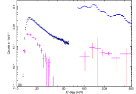
Figure 2: The X-ray spectra in OBS2014 with Suzaku HXD PIN (below 60 keV) and GSO (above 80 keV). Crosses in black and blue represent the raw data and the NXB models, respectively. The background subtracted spectra with statistical errors ($1\sigma$) are shown in magenta. Similarly, those with systematic errors of NXB models are shown in red; the systematic error for PIN is set to be 3% of non X-ray background level (Fukazawa et al., 2009) whereas those for GSO data are determined by each channel as summarized in Table 2.

3.2 ULX and CXB contaminations

We now discuss in more detail the GSO signals in the three energy bins (iv), (v), (vi) in Table 2, which corresponds to the 170 – 350 keV band, which turn out to be most significant in Figure 2. In these GSO energy bands, any possible SN2014J signal could be contaminated from the ULX M82 X-1 signal and Cosmic X-ray background (CXB) emission.

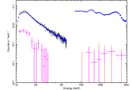
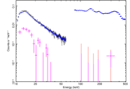
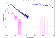
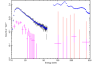
Figure 3: Same spectra as Figure 2, but before OBS2014 (see Table 1). Panels from the top to bottom represent the X-ray spectra in OBSID = 100033010, 100033020, 100033030, and 702026010, respectively.

The hard X-ray emission from M82 X-1 can be estimated by the direct and simultaneous measurements with HXD PIN in the 13 – 70 keV band. The PIN spectrum in OBS2014 is well described by the single power law model, which is usually used for a ULX (Miyawaki et al., 2009). The best fit model has a photon index of $3.93_{-0.40}^{+0.43}$ and an X-ray flux of $1.59_{-0.08}^{+0.06}\times 10^{-11}$ erg cm^-2 s^-1 in the 13 to 70 keV band with a reduced $\chi^{2}$ of 0.80 under 12 degrees of freedom. Instead, the multi-color disk model (Mitsuda et al., 1984) is also used to represent the ULX spectra in several phases, and is always below the power-law model in the harder X-ray band. We therefore consider above power-law estimation as conservative, and the value above corresponds to the upper limit of the contribution of M82 X-1 in the GSO band by an extrapolation from the best-fit power-law model in the PIN band. In addition, the ULXs is usually variable (Miyawaki et al., 2009) as is also seen in Figure 4, but the uncertainty on the flux from the PIN measurement here is about 5 %. Therefore, the contamination from ULX is about $<1.0\pm 0.2$ % of the GSO signal in the 170–350 keV band.

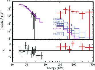
Figure 4: Top panel represents the same plots as red crosses of Figure 2 (i.e., PIN and GSO spectra taken in OBS2014, which are shown in black and red, respectively, in this plot), with the best-fit power-law model in magenta to reproduce the PIN data. The bottom panel shows the chi values to this model. Similarly, best-fit power-law models determined in other observations (OBSID=100033010, 100033020, 100033030, and 702026010; Miyawaki et al., 2009) are also plotted for GSO in blue.

In Figure 5, the GSO data of OBS2014 is compared with the canonical CXB model by HEAO-1 (Gruber, 1999), which is confirmed with the recent hard X-ray observation with Swift BAT (Ajello et al., 2008). For reference, another CXB model by Boldt (1987) is also plotted but is not valid above the 100 keV band. The CXB models were folded into the data space using the corresponding detector’s angular response, which is consistent with the estimation by a full Monte Carlo simulation on Suzaku spacecraft with the Geant4 toolkit (Terada et al., 2005). The uncertainty on the angular response of GSO is checked by multiple pointing observation of Crab nebula (Kokubun et al., 2007) but is not well derived yet. Therefore, we employ two alternatives; a) pulse height spectrum estimated from CXB model by Gruber (1999) with the angular response, and b) the hard X-ray spectrum with the HXD GSO on the blank sky observations described in Section 3.1 In case a), we put 10 % uncertainty on the CXB spectral model as described in Ajello et al. (2008). As plotted in Figure 5, the X-ray flux in 200 – 500 keV band of these two are consistent with each other within $0.6\sigma$ error, whereas the latter tend to have harder spectral shape (see Section 4.3 for detail). In the next section, we use both spectra for the CXB emission and then combine the two results to include systematic errors for the CXB estimation.

An additional systematic uncertainty may arise from the contribution of the Earth albedo emission in the NXB model estimated from the Earth occultation data. This is not considered in the current NXB model by Fukazawa et al. (2009). The X-ray spectrum of the Earth albedo emission can be separated from the CXB spectra by changing the coverage of the Earth within the field of view as has been done by the Swift BAT detector (Ajello et al., 2008), but this method does not work for the HXD GSO in principle because of the design concept of the narrow field-of-view detector (Takahashi et al., 2007). Using the dependence of the Earth albedo level on the geomagnetic latitudes and the inclination angle $i$ of the spacecraft orbit to the Earth equator, the albedo for Suzaku at $i$ = 31 deg is simply interpolated between the Swift measurement (Ajello et al., 2008) at $i=20$ deg and balloon experiments at the polar and at the equator (Imhof et al., 1976). In this interpolation, we assume a systematic error of 25%. Such albedo emission in the NXB model contributes to increase a signal level compared with the CXB emission, but at only about 10% of the CXB level by Gruber (1999), as plotted in Figure 5. Therefore, this causes about 1 % uncertainty for the GSO signal.

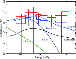
Figure 5: Red crosses represent the NXB-subtracted GSO spectrum for OBS2014 considering the Earth albedo emission in the NXB model (see the text). The error bar includes statistical errors and systematic errors of the NXB model and Earth albedo estimation. The Cosmic X-ray backgrounds with HEAO-1 reported by Boldt (1987) and Gruber (1999) are shown in blue lines, and the Earth albedo estimated for Suzaku from the Swift and balloon experiments (Ajello et al., 2008; Imhof et al., 1976) is shown in black line. X-ray spectrum of GSO taken in blank sky observations (listed in Table 3 with total exposure of 4.49 M sec) is also plotted in blue crosses, where the error bars contain systematic errors in the NXB model and the Earth albedo. Green line represents the ULX spectrum estimated by HXD PIN (same as magenta line in Figure 4). In conversion from CXB model into the data space, we used the GSO response matrix for a flat field emission, accumulated effective areas in the Auxiliary-Response-File (ARF) database in CALDB (ae_hxd_gsoart_20051126.fits).

In summary, we have to subtract contributions of ULX and CXB emission from the GSO signals and add the Earth’s albedo to them of OBS2014 and the blank-sky observation (not to CXB models). Numerically, the contributions of ULX, a) CXB (Gruber, 1999) or b) blank sky spectrum, and the Earth albedo emission to the NXB-subtracted GSO signals (albedo emission added) are 1%, 49%, 39%, and 3%, respectively, in the 170 – 250 keV band. Therefore, the GSO signal towards M82 in 2014 still remains at 4.0 or 2.5 $\sigma$ significance for case a) and b), respectively, in the 170 – 250 keV band i.e., energy bins (iv) and (v) in Table 2, even after subtraction of the ULX and CXB emissions.

3.3 Hard X-ray flux from SN2014J

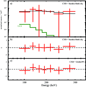
Figure 6: The top panel a) represents the X-ray spectrum of OBS2014 whose NXB and blank sky spectrum (blue crosses in Figure 5) are subtracted and the Earth albedo emission (black line in Figure 5) is added. The error bars include the statistical errors and systematic errors of the NXB model and Earth albedo estimation. Contamination of ULX signals estimated by HXD PIN is shown in green (same as green line in Figure 5), which is fixed as a spectral model in the fitting. Black line shows the best-fit power-law spectrum for the GSO data, and the the chi values are plotted on the second panel b). The bottom panel c) shows the same plot as b) but the HEAO-1 result by by Gruber (1999) is used for the subtraction of Cosmic X-ray background from the GSO data in the fitting, instead of the blank sky data. In this fitting, the statistical errors and systematics of NXB model, CXB model, and the Earth albedo estimations are considered.

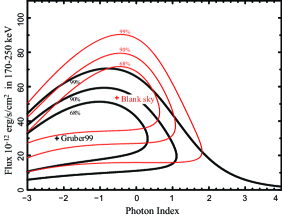
Figure 7: Confidence contour between the photon index and the X-ray flux in the 170 – 250 keV band for the fitting of GSO data of OBS2014 in Figure 6. Red or black lines represent the contour from two fitting cases when the blank-sky data or HEAO-1 Model by Gruber (1999) are used as the Cosmic X-ray background level, respectively. The + marks show the best fit values, and the the contours indicate the 68%, 90%, and 99% levels from the inner to the outside.

In order to derive the X-ray flux from GSO signals numerically, we performed spectral fittings with a power-law model on the GSO spectrum after the subtraction of the NXB (Section 3.1) and the CXB with consideration of the Earth albedo (Section 3.2). We tried two cases of CXB models (cases a) and b) in Section 3.2) to represent uncertainties of the CXB in the fitting. The best fit models are shown in Figure 6 and the hard X-ray flux in the 170 – 250 keV band is found as $(0.9_{-0.3}^{+0.4})\times 10^{-4}$ ph s^-1 cm^-2 or $(1.6\pm 0.4)\times 10^{-4}$ ph s^-1 cm^-2 for cases a) and b) with $1\sigma$ errors, respectively. As shown in Figure 7, the normalization of the power-law model becomes zero at 99% significance level for case a) and the significance of the measured signal is about 90% confidence level (i.e., $2\sigma$) in total, as already described in section 3.1. Therefore, we conclude that the Suzaku constain the X-ray flux of SN2014J to below $2.2\times 10^{-4}$ ph s^-1 cm^-2 at the 170 – 250 keV band ($3\sigma$ limit).

4 Discussion

4.1 Detection of $\gamma-$rays with Suzaku

From the hard X-ray observation of SN2014J with Suzaku HXD at $t=77\pm 2$ days after the explosion (Section 2), the hard X-ray flux in the 170 – 250 keV band is constrained with the 99% ($3\sigma$) upper limit of $<2.2\times 10^{-4}$ ph s^-1 cm^-2. This measurement complements the INTEGRAL measurements of soft X-ray band flux, at similar sensitivity obtained with a shorter exposure.

The Suzaku upper limit at $77\pm 2$ days is consistent with those reported by INTEGRAL for the continuum emission in the 200 – 400 keV band at $(2.0\pm 0.8)\times 10^{-4}$ ph s^-1 cm^-2 at $75\pm 25$ days within errors if we correct the energy width assuming a flat spectrum as indicated by the spectral models of Maeda et al. (2012). If we take the 68% confidence levels (i.e., equivalent to the $1\sigma$ errors) in the systematic and statistical uncertainties of the Suzaku measurement, the X-ray flux becomes $(1.2\pm 0.7)\times 10^{-4}$ ph s^-1 cm^-2 in the same energy range. This is consistent with INTEGRAL results within uncertainties. The consistency can be found in Figure 8, which shows the photon spectra estimated by the best-fit power-law models in cases a) and b), compared with the spectra by Churazov et al. (2015).

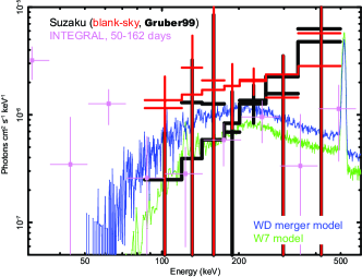
Figure 8: Red and black plots represent the photon spectra converted from the raw spectra in Figure 6, assuming the power-law model with the best-fit values for the data whose CXB component are set to the blank sky data (see the text) or the spectral model by Gruber (1999), respectively. Crosses and lines for them represent the data and the best-fit models, respectively. For reference, photon spectra with the INTEGRAL ISGRI at 50 – 162 days (Figure 8 blue in Churazov et al., 2015) is also plotted in magenta crosses. Green and blue lines shows the spectral models of W7 (Maeda et al., 2012) and the white dwarf merger (Summa et al., 2013), respectively, at the 75 days after the explosion with the ⁵⁶Ni mass of $\sim 0.6M_{\odot}$.

4.2 Type Ia SN models

At $\sim 70$ days after the SN Ia explosion, decays of ⁵⁶Co to ⁵⁶Fe provide a major input into high energy radiation and thermal energy of the SN ejecta. The strongest lines are those at 847 keV and 1238 keV. The annihilation of positrons from this $\beta+$ decay also produces either strong lines at or continuum below $511$ keV. This high-energy radiation is degraded to lower energy by Compton scattering, and below $\sim 200$ keV the photons are absorbed by photoelectric absorption. These processes create characteristic continuum emission from SNe Ia in the hard X-ray and soft gamma-ray regimes.

Figure 8 shows the photon spectrum obtained by the Suzaku observation. This photon spectrum is constructed assuming a power law, and with the assumption of the best-fit power-law models either by a) the CXB model by Gruber (1999) or by b) the blank sky observations. In the same figure, the synthetic spectra of the W7 model (Maeda et al., 2012) and the violent merger model of a $0.9M_{\odot}$ and a $1.1M_{\odot}$ WD (Summa et al., 2013) are compared. In these models, the ⁵⁶Ni-rich region, as well as the layers of intermediate-mass elements above the ⁵⁶Ni-rich region, serve as the Compton-scattering layers. The W7 and delayed detonation models are (more or less) spherical, while the merger model has a large asymmetry in the distribution of the ejected material. In Figure 8, we only show the angle-averaged model spectra; the viewing angle effect is considered later. Both models have $M$(⁵⁶Ni) $\sim 0.6M_{\odot}$, which is consistent with what is inferred from optical properties (e.g., peak luminosity) of SN 2014J (Ashall et al., 2014).

The photon flux at 170-250 keV, taking our $2\sigma$ signal, is indeed consistent with these models, within a systematic error related to the CXB. Above $\sim 300$ keV, the nominal flux level in the Suzaku spectrum is above the level of the CXB (for both CXB models), leaving no residual SN2014J signal contribution, within uncertainties.

The most important difference in these two models is the total mass of the exploding system. The W7 model (Nomoto, 1982) is a representative of an explosion of a single Chandrasekhar-mass WD and the expected $\gamma$-ray emission is similar to other model variants such as deflagration-detonation models in a Chandrasekhar-mass (Maeda et al., 2012). On the other hand, in the violent merger model both of the (sub-Chandrasekhar-mass) WDs are disrupted, leading to the super-Chandrasekhar mass for this particular model presented here (Pakmor et al., 2012; Röpke et al., 2012; Summa et al., 2013). In terms of the expected $\gamma$-ray signals, the two models are characterized by different optical depth to $\gamma$-rays through Compton scattering. The violent merger model has more massive ejecta and thus is more opaque (by a factor of about two), leading to a higher level of Compton continuum in the energy range of Suzaku observations. This difference is seen in Figure 8.

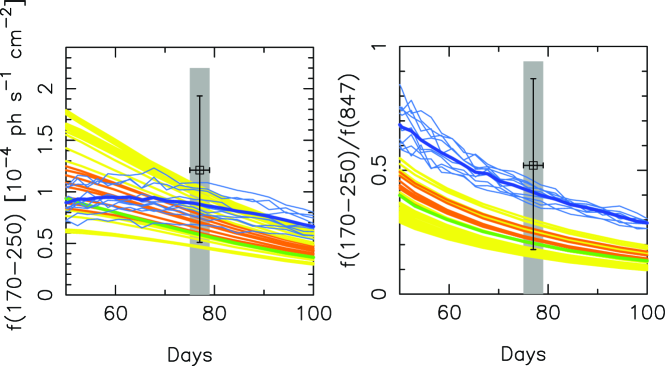
Figure 9: The model light curves from some SN Ia models are compared with the Suzaku observations result. The upper panel shows the flux integrated in the energy of $170-250$ keV, while the lower panel shows the ratio of the $170-250$ keV flux to the 847 keV line flux. The $3\sigma$ upper limit is shown by a gray area, while the flux of the marginal detection is shown by an open square with an error of $1\sigma$. The models shown here are the W7 model (green: Nomoto, 1982), two-dimensional delayed-detonation models with various ignition conditions (yellow and orange: Maeda et al., 2010, 2012), and a violent merger of a $1.1M_{\odot}$ and a $0.9M_{\odot}$ WD (cyan and blue: Röpke et al., 2012; Summa et al., 2013). For the violent merger model, the same model viewed from different directions (cyan) are shown together with an angle-averaged emission (blue). For the delayed-detonation models, the angle-variation is not large at these epochs, and only angle-averaged behaviors are shown for 32 models covering a range of $M$(⁵⁶Ni). Models with $M$(⁵⁶Ni) $=0.47-072M_{\odot}$, which are compatible to observational features of SN 2014J (Ashall et al., 2014), are shown by orange curves, while the other models with larger/smaller $M$(⁵⁶Ni) are shown by yellow curves.

Figure 9 shows the light curves integrated in the energy range of $170-250$ keV for various models, as well as the evolution of the ratio of the same continuum flux to the 847 keV line flux. The Suzaku upper limit and $1\sigma$ data are also plotted as an one snapshot point at $t=77\pm 2$ days thanks to the low-background capability of the HXD. For the ratio, we took the flux from the INTEGRAL observation at $t=75\pm 25$ days after the explosion (Churazov et al., 2014). We adopt the energy range of $170-250$ keV since this corresponds to the marginally detected signal by Suzaku at $2\sigma$. Shown in the figure are the W7 model, 2D delayed detonation models (Maeda et al., 2012) and the violent merger model of Pakmor et al. (2012) for which gamma-ray observables have been presented by Summa et al. (2013). The delayed detonation models were computed for different initial conditions (always with the assumption of a Chandrasekhar-mass WD), covering a wide range of $M$(⁵⁶Ni). The models with $M$(⁵⁶Ni) $=0.47-0.72M_{\odot}$ are indicated by yellow curves, and the W7 model and the violent merger model both have $\sim 0.6M_{\odot}$ of ⁵⁶Ni synthesized in the explosion. These are models compatible to the optical features of SN 2014J. The emission from the violent merger model is sensitive to the viewing angle even at $\sim 60-80$ days, and thus this is shown for various viewing angles.

It is seen that for a similar amount of ⁵⁶Ni, the violent merger model having super-Chandrasekhar mass in the total ejecta, predicts a larger flux than the models with Chandrasekhar-mass WD progenitors. This is a result of the larger optical depth as explained above. Within the observational error, all the models are consistent with the Suzaku data.

The difference between the violent merger model and the other explosion models becomes clearer in the evolution of the flux ratio. Indeed, the ratio of the continuum flux to the line flux has been suggested to be a diagnostic to distinguish the progenitor WD mass (Sim & Mazzali, 2008; Summa et al., 2013) – In case of two models producing the similar amount of ⁵⁶Ni, a larger amount of material surrounding the radioactive isotopes (for the larger WD mass) will convert a larger fraction of the line flux to the Compton down-scattered continuum flux. Therefore the ratio of the continuum to the line flux directly mirrors the ejecta mass. This shows that it is in principle possible to constrain the total mass of the ejecta, thus the mass of the progenitor WD, through $\gamma$-ray observations. Unfortunately, the uncertainty in the Suzaku observation turned out to be too large to discriminate the models, even if we adopt the $1\sigma$ error rather than the $3\sigma$ upper limit. Unfortunately no constraint is obtained at a $3\sigma$ level, but it could already start to constrain some extreme models while at a $1\sigma$ level; the ratio predicted for some 2D delayed detonation models is below the Suzaku point beyond $1\sigma$ error (i.e., the yellow lines below the data point in the lower panel of Figure 9), irrespective of the CXB model. All of these models have $M$(⁵⁶Ni) $>1M_{\odot}$. These models have an extended distribution in ⁵⁶Ni, and thus have small optical depths, leading to a low ratio. We thus reject, while at a $1\sigma$ level, the models with such a large amount of ⁵⁶Ni from the $\gamma$-ray signal alone fully independently of the optical emission.

4.3 CXB measurement with the HXD

Very few models are reported for CXB emission in an energy band above 100 keV. In Section 3.2, the hard X-ray spectrum with the HXD GSO in the 100 – 500 keV band is presented in Figure 5 and compared with the canonical CXB model by Gruber (1999). In the following fittings, the Earth’s albedo emission estimated in Section 3.1 is added to the NXB-subtracted spectrum of the blank sky observations. Overall uncertainties on CXB model (10 % from Ajello et al. (2008)), angular response matrix (4 % due to shade structure opaque to the sun in the X-ray mirror in Figure 11 of Terada et al. (2005)), NXB estimation (0.19% from Section 3.1), and Earth’s albedo emission (25% from Section 3.1), are also included. If we assume that the spectral shape of CXB is given by Gruber (1999), the X-ray flux of the HXD/GSO blank-sky observation becomes $0.7\pm 0.2$ times larger than the value of Gruber model. Numerically, it is $(2.8\pm 0.8)\times 10^{-2}$ ph s^-1 cm^-2 str^-1 or $(1.3\pm 0.3)\times 10^{-8}$ erg s^-1 cm^-2 str^-1 in the 200 – 500 keV band, where the errors represent statistics only. If we reproduce the blank-sky spectrum with a simple power-law model, the photon index becomes harder than that of Gruber (1999) at $1.2^{+1.3}_{-1.0}$ and the X-ray flux becomes consistent with Gruber (1999) at $(5.1^{+2.5}_{-2.6})\times 10^{-2}$ ph s^-1 cm^-2 str^-1 or $(2.6\pm 1.3)\times 10^{-8}$ erg s^-1 cm^-2 str^-1 in the 200 – 500 keV band, whereas the Gruber model corresponds to $4.1\times 10^{-2}$ ph s^-1 cm^-2 str^-1 or $1.9\times 10^{-8}$ erg s^-1 cm^-2 str^-1 in the same energy band. Therefore, the X-ray spectrum of the blank sky observation with GSO reproduces the CXB model by Gruber (1999) within statistical errors.

4.4 Future Perspectives

A next-generation X-ray satellite Hitomi (named ASTRO-H before launch; Takahashi et al., 2014) has been successfully launched on 17 Feb 2016 and higher sensitivities than those of the HXD PIN/GSO or SPI/ISGRI on INTEGRAL will be achieved soon. The background level of the soft gamma-ray detector (SGD; Tajima et al., 2010; Watanabe et al., 2012; Fukazawa et al., 2014) onboard Hitomi will be reduced by one order of magnitude compared to the HXD and therefore soft $\gamma$-ray spectra from a future close-by Type-Ia SNe can be precisely measured as demonstrated in Maeda et al. (2012). Thus, we can distinguish the explosion models between single and double degenerate progenitors as indicated in Figure 9. In distinctions of explosion models on Figure 9, Suzaku demonstrated the importance of the snapshot measurement achieving high sensitivity in a shorter exposure ($\pm 2$ days) than INTEGRAL ($\pm 25$ days). In addition, we demonstrated in this paper that for future observations the refinement of the CXB spectral model is of critical importance.

References

- Ajello et al. (2008) Ajello, M., Greiner, J., Sato, G., et al. 2008, ApJ, 689, 666
- Ambwani & Sutherland (1988) Ambwani, K., & Sutherland, P. 1988, ApJ, 325, 820
- Arnett (1979) Arnett, W. D. 1979, ApJ, 230, L37
- Ashall et al. (2014) Ashall, C., Mazzali, P., Bersier, D., et al. 2014,MNRAS, 445, 4427
- Ayani (2014) Ayani, K. 2014, Central Bureau Electronic Telegrams, 3792, 1
- Baade (1938) Baade, W. 1938, ApJ, 88, 285
- Boldt (1987) Boldt, E., 1987, IAU Symposium, 124, 611
- Cao et al. (2014) Cao, Y., Kasliwal, M. M., McKay, A., Bradley, A., 2014, Astronomers Telegram, 5786
- Churazov et al. (2014) Churazov, E. et al., 2014, Nature, 512 406
- Churazov et al. (2015) Churazov, E., Sunyaev, R., Isern, J., et al. 2015, arXiv:1502.00255
- Dalcanton et al. (2009) Dalcanton, J. J., Williams, B. F., Seth, A. C., et al. 2009, ApJS, 183, 67
- Diehl et al. (2014) Diehl, R. et al., 2014, Science, 345, 1162
- Diehl et al. (2015) Diehl, R. et al., 2015, A&A, 574, A72
- Imhof et al. (1976) Imhof, W. L., Nakano, G. H., & Reagan, J. B. 1976, J. Geophys. Res., 81, 2835
- Itoh et al. (2014) Itoh R., Takaki K., Ui T., Kawabata K. S., M. Y., 2014, Cent. Bur. Electron. Telegrams, 3792, 1
- Karachentsev & Kashibadze (2006) Karachentsev, I. D., & Kashibadze, O. G. 2006, Astrophysics, 49, 3
- Kokubun et al. (2007) Kokubun, M., Makishima, K., Takahashi, T., et al. 2007, PASJ, 59, 53
- Fossey et al. (2014) Fossey, J., Cooke, B., Pollack G., et al, 2014, Central Bureau Electronic Telegrams No. 3792
- Fukazawa et al. (2009) Fukazawa, Y., Mizuno, T., Watanabe, S., et al. 2009, PASJ, 61, 17
- Fukazawa et al. (2014) Fukazawa, Y., Tajima, H., Watanabe, S., et al. 2014, Proc. SPIE, 9144, 91442C
- Georgii et al. (2002) Georgii, R., Plüschke, S., Diehl, R., et al. 2002, A&A, 394, 517
- Gruber (1999) Gruber, D. E. et al. 1999, ApJ, 520, 124
- Hillebrandt & Niemeyer (2000) Hillebrandt, W., & Niemeyer, J. C. 2000, ARA&A, 38, 191
- Iben & Tutukov (1984) Iben, I., Jr., & Tutukov, A. V. 1984, ApJS, 54, 335
- Isern et al. (2013) Isern, J., Jean, P., Bravo, E., et al. 2013, A&A, 552, A97
- Katsuda et al. (2015) Katsuda, S., Mori, K., Maeda, K., et al. 2015, ApJ, 808, 49
- Koyama et al. (2007) Koyama, K., et al., 2007, PASJ, 59, S23
- Leising et al. (1995) Leising, M. D., Johnson, W. N., Kurfess, J. D., et al. 1995, ApJ, 450, 805
- Lichti et al. (1994) Lichti, G. G., Bennett, K., den Herder, J. W., et al. 1994, A&A, 292, 569
- Lichti et al. (1996) Lichti, G. G., Iyudin, A., Bennett, K., et al. 1996, A&AS, 120, 353
- Maeda et al. (2010) Maeda, K., Röpke, F.K., Fink, M., Hillebrandt, W., Travaglio, C., Thielemann, F.-K. 2010, ApJ, 712, 624
- Maeda et al. (2012) Maeda, K., Terada, Y., Kasen, D., et al. 2012, ApJ, 760, 54
- Maoz, Mannucci, and Nelemans (2014) Maoz, D. and Mannucci, F. and Nelemans, G. 2014, ARA&A, 52, 107
- Margutti et al. (2014) Margutti, R. 2014, ApJ, 790, 52
- Milne et al. (2004) Milne, P.A., Hungerford, A.L., Fryer, C.L., et al. 2004, ApJ, 613, 1101
- Mitsuda et al. (1984) Mitsuda, K., Inoue, H., Koyama, K., et al. 1984, PASJ, 36, 741
- Mitsuda et al. (2007) Mitsuda, K., Bautz, M., Inoue, H., et al. 2007, PASJ, 59, 1
- Miyawaki et al. (2009) Miyawaki, R., Makishima, K., Yamada, S., et al. 2009, PASJ, 61, 263
- Nielsen et al. (2014) Nielsen, M. T. B. et al., 2014, MNRAS, 442, 3400
- Nomoto (1982) Nomoto, K. 1982, ApJ, 253, 798
- Pakmor et al. (2010) Pakmor, R., Kromer, M., Röpke, F.K., et al. 2010, Nature, 463, 61
- Pakmor et al. (2012) Pakmor, R., Kromer, M., Taubenberger, S., et al. 2012, ApJ, 747, L10
- Perlmutter et al. (1999) Perlmutter, S. et al., 1999, ApJ, 517, 565
- Phillips et al. (1993) Phillips, M. M. 1993, ApJ, 413, L105
- Riess et al. (1998) Riess, A.G., Filippenko, A.V., Challis, P., et al. 1998, AJ, 116, 1009
- Röpke et al. (2012) Röpke, F.K., Kromer, M., Seitenzahl, I.R., et al. 2012, ApJ, 750, L19
- Scalzo et al. (2014) Scalzo, R.A., Ruiter, A.J., Sim, S.A. 2014, MNRAS, 445, 2535
- Siegert & Diehl (2015) Siegert, T., & Diehl, R. 2015, arXiv:1501.05648
- Sim & Mazzali (2008) Sim, S.A., Mazzali, P.A. 2008, MNRAS,385, 1681
- Sim et al. (2012) Sim, S. A., Fink, M., Kromer, M., et al. 2012, MNRAS, 420, 3003
- Summa et al. (2013) Summa, A., Ulyanov, A., Kromer, M., et al. 2013, A&A, 554, A67
- Tajima et al. (2010) Tajima, H., Blandford, R., Enoto, T., et al. 2010, Proc. SPIE, 7732, 773216
- Takahashi et al. (2007) Takahashi, T., et al., 2007, PASJ, 59, S35
- Takahashi et al. (2014) Takahashi, T., Mitsuda, K., Kelley, R., et al. 2014, Proc. SPIE, 9144, 914425
- Terada et al. (2005) Terada, Y., Watanabe, S., Ohno, M., et al. 2005, IEEE Transactions on Nuclear Science, 52, 902
- The & Burrows (2014) The, L.-S., & Burrows, A. 2014, ApJ, 786, 141
- Watanabe et al. (2012) Watanabe, S., Tajima, H., Fukazawa, Y., et al. 2012, Proc. SPIE, 8443, 844326
- Webbink (1984) Webbink, R. F. 1984, ApJ, 277, 355
- Whelan & Iben (1973) Whelan, J., & Iben, I., Jr. 1973, ApJ, 186, 1007
- Yamaguchi et al. (2015) Yamaguchi, H., et al. 2015, ApJ, 801, 31
- Zheng et al. (2014) Zheng, W., Shivvers, I., Filippenko, A. V., et al. 2014, ApJ, 783, L24