Bond chaos in spin glasses revealed through thermal boundary conditions

Abstract

Spin glasses have competing interactions that lead to a rough energy landscape which is highly susceptible to small perturbations. These chaotic effects strongly affect numerical simulations and, as such, gaining a deeper understanding of chaos in spin glasses is of much importance. The use of thermal boundary conditions is an effective approach to study chaotic phenomena. Here, we generalize population annealing Monte Carlo, combined with thermal boundary conditions, to study bond chaos due to small perturbations in the spin-spin couplings of the three-dimensional Edwards-Anderson Ising spin glass. We show that bond and temperature-induced chaos share the same scaling exponents and that bond chaos is stronger than temperature chaos.

I Introduction

Chaos is a common phenomenon in nonlinear dynamical systems. Interestingly, complex systems with quenched disorder and frustration often display chaotic behavior in one form or another. For example, in spin glasses, the thermodynamic state in thermal equilibrium can change chaotically when an external parameter, e.g., the temperature is tuned. This is also the case for small perturbations of the couplings between the spins, as well as random time-dependent local biases (field chaos). The corresponding chaotic phenomena are therefore called temperature chaos McKay et al. (1982); Kondor (1989); Parisi (1984); Fisher and Huse (1986); Bray and Moore (1987); Ritort (1994); Rizzo and Crisanti (2003); Rizzo and Yoshino (2006); Sasaki and Martin (2003); Sasaki et al. (2005); Katzgraber and Krzakala (2007); Thomas et al. (2011); Fernandez et al. (2013); Wang et al. (2015a), i.e., when the temperature is changed, and bond chaos Sasaki et al. (2005); Katzgraber and Krzakala (2007), when the interactions between the spins are changed. Chaos is believed to be related to hysteresis phenomena, memory and rejuvenation effects in spin glasses Fisher and Huse (1991); Sales and Yoshino (2002); da Silveira and Bouchaud (2004); le Doussal (2005), as well as the generic computational hardness of disordered systems Fernandez et al. (2013); Wang et al. (2015b); Martin-Mayor and Hen (2015). Therefore, chaos is related to both the equilibrium and nonequilibrium properties of dynamical systems. Chaos is also of paramount importance in analog optimization machines, such as the D-Wave Systems Inc. D-Wave 2X quantum annealer. Given the intrinsic analog implementation of the device, small problem misspecifications might lead to the solution of a different Hamiltonian altogether. While temperature is well controlled in these analog machines, precisely encoding the spin-spin interactions (or qubit-qubit couplers) has proven to be difficult due to the limited precision of the device. Given the importance of bond chaos to these novel computing paradigms Zhu et al. (2016); Martin-Mayor and Hen (2015), in this work we investigate bond chaos of spin glasses as a prototypical example of the effects of changing the quenched disorder – a problem far less studied than temperature chaos.

One intriguing numerical result Sasaki et al. (2005); Katzgraber and Krzakala (2007) is that temperature chaos and bond chaos Krza̧kała and Bouchaud (2005) appear to follow the same scaling properties, and that bond chaos is considerably stronger than temperature chaos. However, these observations were left unexplained in Refs. Sasaki et al. (2005); Katzgraber and Krzakala (2007). Here, we provide simple explanations of both results within the framework of the droplet/scaling picture Fisher and Huse (1986, 1988, 1988); Bray and Moore (1986); McMillan (1984) by assuming that temperature chaos is mainly entropy driven, whereas bond chaos is mainly energy driven. Previous work have studied chaotic effects using correlation and overlap functions between different parameters. Here we use an alternate approach: we study bond chaos using thermal boundary conditions Wang et al. (2014, 2015b), in which all $2^{d}$ combinations of periodic and anti-periodic boundary conditions in the $d$ directions (space dimensions) appear in the simulation with their appropriate Boltzmann weights. In this setting, the weights of boundary condition crossings mimic the exchange of dominance of the more abstract pure states. Furthermore, we generalize the population annealing (PA) Monte Carlo Hukushima and Iba (2003); Zhou and Chen (2010); Machta (2010); Wang et al. (2015c) algorithm to simulate bond chaos in glassy systems. One advantage of this approach is that many disorder realizations up to a small perturbation can be studied in a single simulation run, yet have enough dynamical range in the perturbations to study the scaling properties of chaotic effects.

The paper is organized as follows. We first discuss the model, simulation methods, and scaling properties of bond chaos in Sec. II, followed by numerical results on bond chaos compared to previous results on temperature chaos in Sec. III. Concluding remarks are stated in Sec. IV.

II Models and methods

In this section we review technical details of our study, such as the model, numerical and analysis methods, as well as simulation details.

II.1 Model

We simulate the three-dimensional Edwards-Anderson (EA) Ising spin glass represented by the Hamiltonian

$$H=-\sum\limits_{\langle ij\rangle}J_{ij}S_{i}S_{j},$$ (1)

where $S_{i}\in\{\pm 1\}$ are Ising spins. The sum $\langle ij\rangle$ is over the nearest neighbor sites in a cubic lattice with $N=L^{3}$ sites. The coupling $J_{ij}$ between spins $S_{i}$ and $S_{j}$ is chosen from a Gaussian distribution with mean $0$ and variance $1$. We refer to each disorder realization, ${\mathcal{J}}=\{J_{ij}\}$, as a “sample.”

II.2 Generalized population annealing Monte Carlo

We use population annealing to obtain equilibrium states at a low temperature $T=1/\beta$ for a fixed disorder realization ${\mathcal{J}}$ and then obtain equilibrium states as the couplings are continuously transformed from ${\mathcal{J}}$ to ${\mathcal{J}}^{\prime}$ while $T$ is kept fixed. Reference Wang et al. (2015c) provides a detailed description of population annealing Monte Carlo (hereafter referred to as PA). First, we briefly review the “standard” population annealing Monte Carlo method for maintaining thermal equilibrium as the temperature is lowered following a given annealing schedule.

Suppose we have an ensemble or population of $R$ independent replicas of the system chosen from the Gibbs distribution for sample ${\mathcal{J}}$ at inverse temperature $\beta=1/T$. We would like to create a population chosen from the Gibbs distribution for sample ${\mathcal{J}}$ at inverse temperature $\beta^{\prime}$, with $\beta^{\prime}>\beta$. To achieve this goal, we resample the population, making copies of low-energy replicas and removing high-energy replicas from the population. If replica $i$ has energy $E_{i}$, then the expected number of copies $\tau_{i}$ to make of replica $i$ is

$$\tau_{i}=\frac{1}{Q}e^{-(\beta^{\prime}-\beta)E_{i}}\;\;\;{\rm with}\;\;\;Q=\frac{1}{R_{0}}\sum\limits_{i}e^{-(\beta^{\prime}-\beta)E_{i}}.$$ (2)

Here, $R_{0}$ is the expected population size. Note that $\tau_{i}$ is proportional to the ratio of the Boltzmann factors at the two temperatures for a system with energy $E_{i}$, normalized such that the sum of the $\tau$’s is equal to the target population size $R_{0}$.

Now suppose we have a population in equilibrium at inverse temperature $\beta$ with interactions ${\mathcal{J}}$ and we would like to transform to a new population at the same temperature $\beta$ but with different couplings ${\mathcal{J}}^{\prime}$. For such a procedure, the resampling now requires that

$$\tau_{i}=\frac{1}{Q}e^{-\beta(E_{i}^{\prime}-E_{i})}\;\;\;{\rm with}\;\;\;Q=\frac{1}{R_{0}}\sum\limits_{i}e^{-\beta(E_{i}^{\prime}-E_{i})}.$$ (3)

In Eq. (3), $E_{i}^{\prime}$ and $E_{i}$ are the energy of replica $i$ with bonds ${\mathcal{J}}^{\prime}$ and ${\mathcal{J}}$, respectively, with the spins in each replica held fixed.

One can summarize Eqs. (2) and (3) using reduced Hamiltonians $\mathcal{H}=\beta H$. For two sets of close (similar) distributions on the same state space with Boltzmann factors of $\exp[-\mathcal{H}_{i}]$ and $\exp[-\mathcal{H}_{i}^{\prime}]$ for replica $i$, when transforming a population of replicas from $\mathcal{H}$ to $\mathcal{H^{\prime}}$,

$$\tau_{i}=\frac{1}{Q}e^{-(\mathcal{H}_{i}^{\prime}-\mathcal{H}_{i})}\;\;\;{\rm with}\;\;\;Q=\frac{1}{R_{0}}\sum\limits_{i}e^{-(\mathcal{H}_{i}^{\prime}-\mathcal{H}_{i})}.$$ (4)

Within this framework, one can perturb the system either by a change in temperature, by a change in the spin-spin interactions, or both using PA. Finally, we note that the free-energy difference can be generalized, too, using the free-energy perturbation method as $-\beta^{\prime}F^{\prime}=-\beta F+\langle\exp[-(\mathcal{H^{\prime}}-\mathcal{H})]\rangle_{\mathcal{H}}$, although the free energy is not needed in this work.

One advantage of PA over other methods such as parallel tempering Monte Carlo Hukushima and Nemoto (1996) is the ease of simulating thermal boundary conditions. In thermal boundary conditions, each of the $2^{d}$ choices of periodic or anti-periodic boundary conditions in each of the $d$ Cartesian directions appears in the ensemble with its correct statistical weight, given by $\exp(-\beta F_{i})$, where $F_{i}$ is the free energy of the system in boundary condition $i$. As described in Ref. Wang et al. (2015c), thermal boundary conditions can be simulated in PA by initiating the population at $\beta=0$ with an equal fraction $1/2^{d}$ of the population is in each of the $2^{d}$ boundary conditions. Thereafter, as the temperature or the bond configuration is modified, resampling changes the relative fraction of each boundary condition. At each value of $\beta$ and $\mathcal{J}$ in the annealing schedule, let $p_{i}$ be the fraction of boundary condition $i$ in the population. The free energy of each boundary condition is then proportional to $-\log p_{i}$. The evolution of $p_{i}$ with bond configuration is our main tool to study bond chaos.

II.3 Scaling analysis and observables

We present the scaling analysis of temperature and bond chaos within the droplet theory of the low-temperature phase of the the Edwards-Anderson Ising spin glass. In this theory, the low-lying excitations of the spin glass are flipped compact droplets. The free energy cost to flip a droplet of size $\ell$ at temperature $\beta$ scales as $\ell^{\theta}$ with disorder ${\mathcal{J}}$, and the free energy cost to perturb the bonds with $\delta{\mathcal{J}}$ for the droplet and the flipped droplet is $\Delta F_{1}$ and $\Delta F_{2}$, respectively. Then the free-energy cost to flip the droplet at ${\mathcal{J}}^{\prime}={\mathcal{J}}+\delta{\mathcal{J}}$ is $\ell^{\theta}+\Delta F_{2}-\Delta F_{1}$, with $\theta$ the stiffness exponent. One can see that the effect of changes in the spin-spin interactions for the last two terms is nonzero only at the surface of the droplet due to spin-reversal symmetry. Because $\Delta F=\Delta E-T\Delta S$, and assuming the energy difference dominates when we change the couplings and therefore, the last two terms scale as $\delta{\mathcal{J}}\ell^{d_{\rm s}/2}$, where $d_{\rm s}/2$ is the fractal dimension of the boundary of the droplet. Putting everything together, the free-energy cost to flip the droplet at ${\mathcal{J}}^{\prime}$ scales as $\ell^{\theta}-\delta{\mathcal{J}}\ell^{d_{\rm s}/2}$, and therefore the strength $\delta{\mathcal{J}}$ needed for bond chaos scales as

$$\delta{\mathcal{J}}\sim\frac{1}{\ell^{\zeta}},$$ (5)

where

$$\zeta=d_{\rm s}/2-\theta.$$ (6)

This simple derivation using droplet arguments suggests that bond chaos effects should be described by the same scaling exponents ($\theta$, $d_{\rm s}/2$ and $\zeta$) as temperature chaos Wang et al. (2015b); Katzgraber and Krzakala (2007).

Following Refs. Wang et al. (2014, 2015b), $\theta$ can be calculated using sample stiffness scaling, $d_{\rm s}/2$ can be calculated using the scaling of energy differences at boundary condition crossings, and $\zeta$ is related to the scaling of the number of dominant crossings. We briefly summarize these quantities and their scaling.

For a sample ${\mathcal{J}}$ at inverse temperature $\beta$, let $f_{{\mathcal{J}},\beta}=\max_{i}\left[p_{i}\right]$ be the fraction of the population in the dominant boundary condition, i.e., the boundary condition with the largest fraction in the population. The sample stiffness $\lambda_{{\mathcal{J}},\beta}$ is defined as

$$\lambda_{{\mathcal{J}},\beta}=\log\frac{f_{{\mathcal{J}},\beta}}{1-f_{{\mathcal{J}},\beta}},$$ (7)

and is an estimator of the free-energy difference (times $-\beta$) between the dominant boundary conditions and all other boundary conditions in sample ${\mathcal{J}}$ at inverse temperature $\beta$. (Henceforth, we leave ${\mathcal{J}}$ and $\beta$ implicit). Let $G_{L}(\lambda)$ be the cumulative distribution function for $\lambda$, then it was shown in Ref. Wang et al. (2014) that the function $1-G_{L}(\lambda)$ is approximately exponential, which then allows for a scaling analysis. Define a characteristic $\lambda_{\rm char}(L)$ such that $1-G(\lambda)=e^{-\lambda/\lambda_{\rm char}}$ and $1-G(\lambda_{\rm char}\log b)=1/b$ for any $b$. The value $b$ should be chosen such that $\lambda_{\rm char}$ is obtained from the tail of the distribution but not so far into the tail where the statistics are poor. For $T=0.5$ (dimensionless units), we choose $b=10$. We have verified that the distribution functions for different linear system sizes $L$ collapse well onto the same curve after being scaled by $\lambda_{\rm char}(L)$. Standard spin stiffness scaling then gives

$$\lambda_{\rm char}\sim L^{\theta}.$$ (8)

A key element of the analysis of both bond chaos and temperature chaos is the identification and analysis of boundary condition crossings, which occur at values of ${\mathcal{J}}$ and $\beta$ where there are two boundary conditions $i$ and $j$ having the same fraction in the population, $p_{i}=p_{j}$. Let $|\Delta E|$ be the absolute value of the energy difference at a boundary condition crossing. Then the scaling of $|\Delta E|$ with the system size $L$ yields the exponent controlling the domain-wall fractal dimension ($d_{\rm s}/2$) according to,

$$\langle|\Delta E|\rangle\sim L^{d_{\rm s}/2}.$$ (9)

Here, the average is over all crossing in a given range of temperature or bond configuration and above a threshold $p_{c}$, such that at the crossing $p_{i}=p_{j}>p_{c}$. We have also used the median of $|\Delta E|$ rather than the mean.

Boundary condition crossings are manifestations of chaos. The scaling of their number with the system size gives access to the chaos exponent $\zeta$. Let $N_{C}$ be the number of dominant crossings in some range of either $\beta$ or $\mathcal{J}$. At a dominant crossing, the two boundary conditions exchange dominance and on either side of the crossing, one of the two boundary conditions is dominant. Dominant crossings, rather than all crossings above an arbitrary threshold, are used to reduce finite-size effects. From $N_{C}$ within some range of $\beta$ or $\mathcal{J}$, we compute $\zeta$ from,

$$N_{C}\sim L^{\zeta}.$$ (10)

The relationship between the exponents presented in Eq. (6), as well as the relative strength of bond and temperature chaos (which corresponds to the ratio of the scaled density of the number of dominant boundary condition crossings $N_{C}$), are examined and discussed in Sec. III.

II.4 Simulation details

We start by discussing how to simulate bond chaos for a single disorder realization. In the reduced Hamiltonian representation, we can either change the inverse temperature $\beta$ or perturb the spin-spin interactions ${\mathcal{J}}$. We use the following procedure to change the interactions: For each disorder realization ${\mathcal{J}}_{0}$, we choose an independent perturbation ${\mathcal{J}}^{\prime}$ and change the original bonds as

$${\mathcal{J}}=\dfrac{{\mathcal{J}}_{0}+c{\mathcal{J}}^{\prime}}{\sqrt{1+c^{2}}},$$ (11)

where $c\in[0,0.1]$ is a small number. In this manner, for each value of the perturbation strength $c$, a Gaussian disorder distribution is preserved Ney-Nifle and Young (1997); Ney-Nifle (1998); Krza̧kała and Bouchaud (2005); Katzgraber and Krzakala (2007).

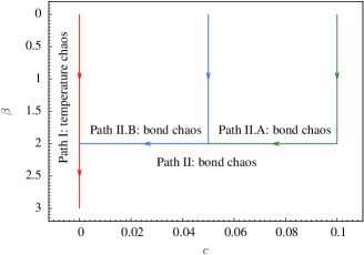
From now on, within the reduced Hamiltonian representation, we vary the parameters $\beta$ and $c$ in the $(\beta,c)$ plane. We start the simulation first with fixed $c$ from $\beta=0$ down to $\beta=2$. This takes the system from the paramagnetic to the spin-glass phase. Following this anneal in temperature, we fix $\beta=2$ and change the bond perturbation strength $c$ in the interval $[0,0.1]$ to induce chaotic effects. To double-check our results, we have chosen the interactions of the unperturbed system, ${\mathcal{J}}_{0}$, from the study of temperature chaos in Ref. Wang et al. (2015b). The perturbed interactions ${\mathcal{J}}^{\prime}$ were chosen independently. We first do a temperature anneal of the system from $\beta=0$ to $\beta=2$ at $c=0.1$ fixed, and then we change $c$ from $0.1$ to $0$. In this way, the final interaction configuration is the same as ${\mathcal{J}}_{0}$, which allows us to compare the results directly to the ones from our temperature chaos study in Ref. Wang et al. (2015b). It is of paramount importance to verify after both simulation paths that the weights of each boundary conditions $\{p_{i}\}$ agree. In our simulations, we require the family entropy $S_{f}\geq\log(100)$ (where $S_{f}$ is a measure of equilibration discussed in Ref. Wang et al. (2015c)) for each path as well as $\max\{|p_{i}-p_{i}^{\prime}|\}\leq 0.05$, where $\{p_{i}\}$ and $\{p_{i}^{\prime}\}$ are the weights of each boundary conditions from the two distinct paths, respectively, for each sample.

Computationally hard samples that do not fulfill the two equilibration criteria were either rerun with a larger population size, or by breaking the bond-chaos $c$ path into two segments, where each segment separately is considerably easier to equilibrate. Figure 1 shows how the $c$ path is split into two pieces (path II.A and II.B). Measurements along path II.B require an additional population annealing run starting at $\beta=0$ and $c=0.05$. Whenever runs are combined, we test the family entropy of each run, as well as the matching of boundary conditions between the different runs.

Figure 1: (Color online) Schematic simulation paths. In all cases, a quench from $\beta=0$ to $\beta=2$ is first performed. For the bond chaos case, an additional set of simulations for $\beta=2$ along the $c$-axis from $c=0.1$ to $c=0$ is performed. Path I (red) represents a simulation to probe temperature chaos. Path II represents a bond chaos simulation. If the sample is computationally difficult, then path II is split into paths II.A (green) and II.B (blue) that are each run independently.

We have carried out a large-scale simulation of bond chaos for linear system sizes $L=4$, $6$, $8$, and $10$, with $2001$ samples for each system size. The details of the simulation parameters are summarized in Table. 1.

Table 1: Parameters of bond-chaos simulations using generalized PA. $L$ is the linear system size, $R_{0}$ is the standard number of replicas, $T_{0}=1/\beta_{0}$ is the lowest temperature simulated, $N_{T}$ is the number of temperature steps (evenly spaced in $\beta$) in the annealing schedule, $N_{b}$ is the number of disorder steps (evenly spaced in $c$) in the annealing schedule, and $n$ is the number of disorder realizations studied.

$L$	$R_{0}$	$T_{0}$	$N_{T}$	$N_{b}$	$n$
$4$	$5\times 10^{4}$	$0.5$	$101$	$51$	$2001$
$6$	$2\times 10^{5}$	$0.5$	$101$	$51$	$2001$
$8$	$5\times 10^{5}$	$0.5$	$201$	$101$	$2001$
$10$	$2\times 10^{6}$	$0.5$	$301$	$101$	$2001$

III Results

III.1 Scaling properties of bond chaos

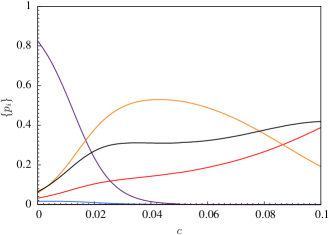
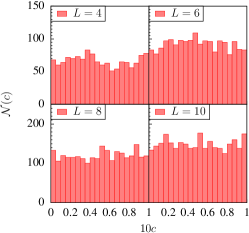
The boundary condition probabilities of a sample of linear size $L=8$ is shown in Fig. 2, displaying chaotic behavior via several boundary condition crossings. In this figure and in the analysis of the energy differences, we have registered crossings above a threshold of $p_{c}=0.1$ when two boundary conditions cross as a function of $c$. Figure 3 shows a histogram of the distribution (i.e., number density) of crossings as a function of $c$, which is relatively flat, as expected. On the other hand, the distribution of the crossings is approximately exponential as a function of $\beta$ when chaotic effects are induced by thermal changes Wang et al. (2015b).

Figure 2: (Color online) Evolution of the relative weights of each boundary conditions, $\{p_{i}\}$, for a chaotic sample of linear system size $L=8$ and $\beta=2$. Different boundary conditions show crossings, i.e., chaotic events. Three of the eight boundary conditions have probabilities too small to be seen on the plot.

Figure 3: (Color online) Distribution of all crossings above a cutoff of $p_{c}=0.1$ as a function of $c$. The distributions are relatively uniform compared to the distributions of temperature chaos Wang et al. (2015b) which are exponential. Note that the horizontal axis has been multiplied by 10 for better viewing.

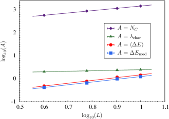
The system-size scaling of the number of dominant crossings $N_{C}$, sample stiffness $\lambda_{\rm{char}}$, mean and median of the energy cost at boundary condition crossings $\langle|\Delta E|\rangle$ and $|\Delta E|_{\rm{med}}$, respectively, are all shown in Fig. 4. We have used data at both $(\beta=2,c=0)$ and $(\beta=2,c=0.1)$ after a temperature anneal for the scaling of $\lambda_{\rm{char}}$ to improve statistics for the measurement of $\theta$. The different exponents can be extracted by linear fits to the data. Our estimates are

$$\theta = 0.22(3)\;,$$ (12)

$$d_{\rm s}/2 = 1.22(3)\;\;\;\;\;\;{\rm(mean)}\;,$$ (13)

$$d_{\rm s}/2 = 1.19(3)\;\;\;\;\;\;{\rm(median)}\;,$$ (14)

$$\zeta = 1.01(4)\;.$$ (15)

Note that $d_{\rm s}/2-\theta=1.00(4)$ (mean) and $d_{\rm s}/2-\theta=0.97(4)$ (median), are in good agreement with $\zeta$. These estimates of the exponents are also in agreement with the results obtained from temperature chaos Wang et al. (2015b), showing that temperature chaos and bond chaos indeed share the same set of scaling exponents.

Figure 4: (Color online) Scaling of the measured quantities as a function of system size. The log-log plot clearly shows that the different quantities are well fit with a power law. The slope of the number of dominant crossings scales as $N_{C}\sim L^{\zeta}$, the energy difference at all registered boundary condition crossings above $p_{c}=0.1$ scales as $\Delta E\sim L^{d_{\rm s}/2}$, and $\lambda_{\rm char}\sim L^{\theta}$. Note that for the energy difference at all registered boundary condition crossings both the median $\Delta E_{\rm med}$ and average $\langle\Delta E\rangle$ have the same slope within error bars. Error bars are smaller than the symbols.

III.2 Comparison of temperature and bond chaos

Next, we compare the relative strength of temperature chaos and bond chaos. A natural quantity to compare is the number of dominant crossings $N_{C}$. However, due to the different types of perturbations (temperature $\beta$ vs interactions $c$), we need to compare fairly the density of crossing with respect to $\beta$ and $c$. Let $\Delta\beta$ be the range of inverse temperatures in the analysis of temperature chaos and $\Delta c$ (here $\Delta c=0.1$) the range of modification of the bond configuration. The relative strength of the perturbation of temperature chaos to bond chaos seen from the reduced Hamiltonian is

$$\frac{\Delta\beta}{\beta\Delta c}.$$ (16)

The distribution of crossings of bond chaos is approximately uniformly distributed, therefore, the density of crossings for bond chaos (BC) is simply given by

$$\rho^{\rm BC}=\frac{{N_{C}}^{\rm TC}}{\beta\Delta c}.$$ (17)

The distribution of crossing for temperature chaos is more complicated and is approximately exponential in the range $\beta\in[\beta_{\rm min},\beta_{\rm max}]=[1.5,3]$ for all system sizes studied in Ref. Wang et al. (2015b). An exponential fit of the form

$${\mathcal{N}}(\beta)=\frac{ae^{-a\beta}}{e^{-\beta_{\rm min}a}-e^{-\beta_{\rm max}a}},$$ (18)

with $\beta\in[1.5,3]$ yields $a\approx 1.12$. This suggests that the density of crossing distributions at $\beta=2$ is approximately $1.18$ times larger than that of the averaged density in the whole temperature range $[1.5,3]$. We note that the ratio depends only very weakly on $a$. The corresponding density of crossings for temperature chaos (TC) is therefore given by

$$\rho^{\rm TC}=\frac{1.18{N_{C}}^{\rm TC}}{\Delta\beta}.$$ (19)

Using $\Delta c=0.1$, $\beta=2$, $\Delta\beta=1.5$, and $N_{C}$ for the whole perturbation range of both types of chaos in Eqs. (17) and (19), we can define a quantity $\kappa$ that quantifies the relative strength of bond chaos and temperature chaos as

$$\kappa = \frac{\rho^{\rm BC}}{\rho^{\rm TC}}$$ (20)

$$\approx 6.34\frac{{N_{C}}^{\rm BC}}{{N_{C}}^{\rm TC}},$$

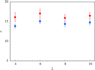
where ${N_{C}}^{\rm BC}$ and ${N_{C}}^{\rm TC}$ are the total number of dominant boundary condition crossings of bond chaos and temperature chaos, respectively. A plot of $\kappa$ as a function of the linear system size $L$ is shown in Fig. 5 (red circles). Note that $\kappa$ is almost a constant function of $L$, as expected from the scaling properties of $N_{C}$. Averaging over the studied system sizes $L$, we find that

$$\kappa\approx 16(1).$$ (21)

Therefore, bond chaos is more than one order of magnitude stronger than temperature chaos at low temperatures ($\beta=2$). It is interesting that our result is very close to the value of $17.5$ quoted in Ref. Sasaki et al. (2005) even though the two values are computed using fundamentally different methods and models. Note that the difference of the threshold to register crossings does not affect the number of dominate boundary condition crossings and therefore also $\kappa$, as in both cases, a dominant boundary condition crossing cannot occur below the chosen threshold, $p_{c}=0.1$ for bond chaos and $p_{c}=0.05$ for temperature chaos.

We propose a simple physical interpretation for $\kappa$. At first sight, one might expect that the scale of $\Delta E$ and $\Delta(TS)$ might be relevant to explain $\kappa$. However, while we find this is indeed a factor—especially at low temperatures—this is not sufficient. We find that the strength of responses of the quantities with respect to $c$ and $\beta$ are more relevant, as chaos is a dynamical process. To this effect, we use an alternate definition of the relative strength $\kappa$, namely

$$\kappa = \left\langle\frac{\partial|\Delta E|}{\beta\partial c}\right\rangle\Big{/}\left\langle\frac{\partial|\Delta(TS)|}{\partial\beta}\right\rangle,$$ (22)

where the derivative is evaluated using finite element methods at the same temperature $\beta=2$. This theoretical prediction of $\kappa$ is also shown in Fig. 5 (blue squares). Note that Eq. (22) also explains why $\kappa$ does not depend on the system size from the same scaling properties of $\Delta E$ and $\Delta(TS)$. The predictions are reasonably close, showing that bond chaos is indeed energy driven, while temperature chaos is entropy driven.

Figure 5: (Color online) Relative strength between bond and temperature chaos, $\kappa$, as a function of system size $L$ computed from Eq. (20) (red circles) and Eq. (22) (blue squares). Using droplet scaling arguments one can show that $\kappa$ does not depend on the system size.

We know that the number of dominant crossings $N_{C}$ is a growing function of system size $L$. It is a natural scenario that the fraction of instances with dominant crossings also grows with $L$, along with the mean number. The fraction of samples with dominant crossings for both temperature chaos and bond chaos are shown in Table. 2.

Table 2: Fraction of instances with dominant crossings as a function linear system size $L$ for temperature chaos (TC) and bond chaos (BC). Note that the fraction of instances with dominant crossings grows with $L$, along with the mean number.

$L$	$4$	$6$	$8$	$10$
TC	0.11(1)	0.16(1)	0.21(1)	0.26(1)
BC	0.27(1)	0.39(1)	0.48(1)	0.56(1)

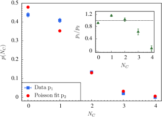
It has been argued that temperature chaos in spin glasses is dominated by rare events Fernandez et al. (2013). By looking at the distribution of the number of dominant crossing for each disorder realization one can study this hypothesis in the context of both bond and temperature chaos. Figure 6 shows the probability with respect to disorder realizations of having $N_{C}$ dominant crossings as a function of $N_{C}$ for the case of bond chaos with $L=10$. The Poisson distribution with the same mean is also shown in Fig. 6. The inset shows the ratio of both distributions. There are systematic deviations between the data and the Poisson distribution, specifically there are fewer $N_{C}=0$ samples than the Poisson distribution and more $N_{C}=1$ samples. More importantly, the probability of getting large values of $N_{C}$ is less than the Poisson prediction. We find qualitatively similar results for both temperature and bond chaos and for all sizes studied. Therefore, in contrast to the results of Ref. Fernandez et al. (2013), our measure of chaos based on boundary condition crossings is not described by an extreme value distribution and is not dominated by rare events.

Figure 6: (Color online) Representative distribution of the number of dominant crossings $N_{C}$ for $L=10$ of bond chaos, along with a Poisson fit. The ratio of the weights of the distribution to the Poisson fit is shown in the inset. One can see that the number of dominant crossings is still dominant by samples with small number of crossings of the majority of instances. Qualitatively similar results have been obtained for temperature chaos, as well as all system sizes studied.

It has recently been established that temperature chaos is associated with computational hardness Fernandez et al. (2013); Wang et al. (2015b); Zhu et al. (2016); Martin-Mayor and Hen (2015). We note that the same can be stated for bond chaos. In Sec. II.4 we divided disorder realizations into two groups: hard to simulate and easy to simulate. We take a closer look at the average number of dominant crossings in each class. For $L=8$, approximately $13\%$ of the instances are typically hard, and the mean number of dominant crossings are $0.92(4)$ and $0.53(2)$ for computationally “hard” and “easy” instances, respectively. For $L=10$, approximately $47\%$ of the instances are hard, and the mean number of dominant crossings are $1.02(3)$ and $0.49(2)$ for hard and easy instances, respectively.

This suggests that the difficulty of transforming an equilibrium state for one set of bonds to another set of bonds is strongly correlated with bond chaos along the path connecting the two bond configurations. This is not unexpected because a crossing indicates that configurations (including both spin and boundary condition) that were important for one set of bonds are no longer as important when the bonds are modified. The fact that both temperature and bond chaos introduce computational hardness, suggests the possibility of optimizing population annealing Monte Carlo for simulating a fixed bond configuration by choosing curved paths in the temperature–disorder space that minimizes chaos. A simulation of disorder realization $\mathcal{J}$ might begin with disorder realization $\mathcal{J}^{\prime}$ and involve annealing in both temperature and bond strength. This idea remains to be explored and might also provide an avenue to overcome gaps in the energy spectrum for quantum annealing simulations.

IV Conclusions

In this work, we have studied bond chaos using thermal boundary conditions via a generalization of population annealing Monte Carlo. We provided a simple explanation as to why temperature chaos and bond chaos share the same set of scaling exponents within the framework of the droplet/scaling picture. We also show quantitatively that bond chaos is approximately one order of magnitude stronger than temperature chaos. A simple physical picture is proposed that explains the relative strength, identifying that bond chaos is energy driven, whereas temperature chaos is entropy driven. As such, the surface of excitations plays a key role in these phenomena. Our work on temperature and bond chaos also establishes the validity of the use of thermal boundary conditions to study chaotic phenomena in disordered systems.

We use this opportunity to emphasize that the fact that bond chaos is so much stronger than temperature chaos should be a source of concern in analog computing machines, such as the D-Wave Systems Inc. DW2X. While slight temperature variations of the device might only affect the encoded problem slightly, small perturbations of the couplers might change the encoded Hamiltonian and yield erroneous results.

We intend to apply the method used here to other paradigmatic spin-glass systems, such as the four-dimensional Edwards-Anderson Ising spin glass. A more challenging and intriguing problem is to investigate field chaos in the mean-field Sherrington-Kirkpatrick model Sherrington and Kirkpatrick (1975)—which also has a spin-glass phase in an external magnetic field—using a generalized definition of boundary conditions.