Convolutional Patch Representations for Image Retrieval: an Unsupervised Approach

Abstract

Convolutional neural networks (CNNs) have recently received a lot of attention due to their ability to model local stationary structures in natural images in a multi-scale fashion, when learning all model parameters with supervision. While excellent performance was achieved for image classification when large amounts of labeled visual data are available, their success for unsupervised tasks such as image retrieval has been moderate so far.

Our paper focuses on this latter setting and explores several methods for learning patch descriptors without supervision with application to matching and instance-level retrieval. To that effect, we propose a new family of convolutional descriptors for patch representation, based on the recently introduced convolutional kernel networks. We show that our descriptor, named Patch-CKN, performs better than SIFT as well as other convolutional networks learned by artificially introducing supervision and is significantly faster to train. To demonstrate its effectiveness, we perform an extensive evaluation on standard benchmarks for patch and image retrieval where we obtain state-of-the-art results. We also introduce a new dataset called RomePatches, which allows to simultaneously study descriptor performance for patch and image retrieval.

Figure 1: Proposed image retrieval pipeline. Interest points are extracted with the Hessian-affine detector (left), encoded in descriptor space (middle), and aggregated into a compact representation using VLAD-pooling (right). The main focus of the paper lies in the choice of the patch-level visual descriptor.

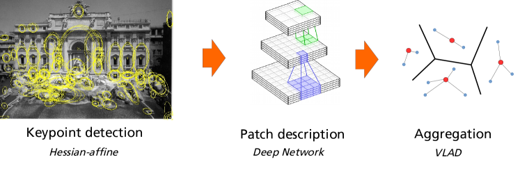
1 Introduction

This paper explores convolutional architectures as robust visual descriptors for image patches and evaluates them in the context of patch and image retrieval. We explore several levels of supervision for training such networks, ranging from fully supervised to unsupervised. In this context, requiring supervision may seem unusual since data for retrieval tasks typically does not come with labels. Convolutional Neural Networks (CNNs) have achieved state-of-the-art in many other computer vision tasks, but require abundant labels to learn their parameters. For this reason, previous work with CNN architectures on image retrieval have focused on using global (Babenko et al, 2014) or aggregated local (Razavian et al, 2014; Gong et al, 2014; Ng et al, 2015; Babenko and Lempitsky, 2015; Tolias et al, 2015) CNN descriptors that were learned on an unrelated classification task. To improve the performance of these transferred features, Babenko et al (2014) showed that fine-tuning global descriptors on a dataset of landmarks results in improvements on retrieval datasets that contain buildings. It is unclear, however, if the lower levels of a convolutional architecture, appropriate for a local description, will be impacted by such a global fine-tuning (Yosinski et al, 2014). Recent approaches have, thus, attempted to discriminatively learn low-level convolutional descriptors, either by enforcing a certain level of invariance through explicit transformations (Fischer et al, 2014) or by training with a patch-matching dataset (Zagoruyko and Komodakis, 2015; Simo-Serra et al, 2015). In all cases, the link between the supervised classification objective and image retrieval is artificial, which motivates us to investigate the performance of new unsupervised learning techniques.

To do so, we propose an unsupervised patch descriptor based on Convolutional Kernel Networks (CKNs)(Mairal et al, 2014b). This required to turn the CKN proof of concept of Mairal et al (2014b) into a descriptor with state-of-the-art performance on large-scale benchmarks. This paper introduces significant improvements of the original model, algorithm, and implementation, as well as adapting the approach to image retrieval. Our conclusion is that supervision might not be necessary to train convolutional networks for image and patch retrieval, since our unsupervised descriptor achieves the best performance on several standard benchmarks.

One originality of our work is also to jointly evaluate our models on the problems of patch and image retrieval. Most works that study patch representations (Brown et al, 2011; Winder et al, 2009; Zagoruyko and Komodakis, 2015; Fischer et al, 2014), do so in the context of patch retrieval only, and do not test whether conclusions also generalize to image retrieval (typically after an aggregation step). In fact, the correlation between the two evaluation methods (patch- and image-level) is not clear beforehand, which motivated us to design a new dataset to answer this question. We call this dataset RomePatches; it consists of views of several locations in Rome (Li et al, 2010), for which a sparse groundtruth of patch matches is obtained through 3D reconstruction. This results in a dataset for patch and image retrieval, which enables us to quantify the performance of patch descriptors for both tasks.

To evaluate the descriptor performance, we adopt the following pipeline (see Fig. 1), described in detail in section 6.1.1. We use the popular Hessian-Affine detector of Mikolajczyk and Schmid (2004), which has been shown to give state-of-the-art results (Tuytelaars and Mikolajczyk, 2008). The regions around these points are encoded with the convolutional descriptors proposed in this work. We aggregate local features with VLAD-pooling (Jégou et al, 2010) on the patch descriptors to build an approximate matching technique. VLAD pooling has been shown to be better than Bag-of-Word, and to give similar performance to Fisher Vectors (Perronnin and Dance, 2007), another popular technique for image retrieval (Jégou et al, 2012).

A preliminary version of this article has appeared in (Paulin et al, 2015). Here we extend the related work (Section 2) and describe in detail the convolutional kernel network (CKN), in particular its reformulation which leads to a fast learning algorithm (Section 4). We also add a number of experiments (see Section 6). We compare to two additional supervised local CNN descriptors. The first one is based on the network of Fischer et al (2014), but trained on our RomePatches dataset. The second one is trained with the Siamese architecture of Zagoruyko and Komodakis (2015). We also compare our approach to an AlexNet network fine-tuned on the Landmarks dataset. Furthermore, we provide an in-depth study of PCA compression and whitening, standard post-processing steps in image retrieval, which further improve the quality of our results. We also show that our method can be applied to dense patches instead of Hessian-Affine, which improves performance for some of the benchmarks.

The remainder of the paper is organized as follows. We discuss previous work that is most relevant to our approach in Section 2. We describe the framework for convolutional descriptors and convolutional kernel networks in Sections 3 and 4. We introduce the RomePatches dataset as well as standard benchmarks for patch and image retrieval in Section 5. Section 6 describes experimental results.

2 Related Work

In this section we first review the state of the art for patch description and then present deep learning approaches for image and patch retrieval. For deep patch descriptors, we first present supervised and, then, unsupervised approaches.

2.1 Patch descriptors

A patch is a image region extracted from an image. Patches can either be extracted densely or at interest points. The most popular patch descriptor is SIFT (Lowe, 2004), which showed state-of-the-art performanceMikolajczyk and Schmid (2005) for patch matching. It can be viewed as a three-layer CNN, the first layer computing gradient histograms using convolutions, the second, fully-connected, weighting the gradients with a Gaussian, and the third pooling across a 4x4 grid. Local descriptors that improve SIFT include SURF (Bay et al, 2006), BRIEF (Calonder et al, 2010) and LIOP (Wang et al, 2011). Recently, Dong and Soatto (2015) build on SIFT using local pooling on scale and location to get state-of-the-art performance in patch retrieval.

All these descriptors are hand-crafted and their relatively small numbers of parameters have been optimized by grid-search. When the number of parameters to be set is large, such an approach is unfeasible and the optimal parametrization needs to be learned from data.

A number of approaches learn patch descriptors without relying on deep learning. Most of them use a strong supervision. Brown et al (2011) (see also Winder et al (2009)) design a matching dataset based on 3D models of landmarks and use it to train a descriptor consisting of several existing parts, including SIFT, GLOH (Mikolajczyk and Schmid, 2005) and Daisy (Tola et al, 2010). Philbin et al (2010) learn a Mahalanobis metric for SIFT descriptors to compensate for the binarization error, with excellent results in instance-level retrieval. Simonyan et al (2014) propose the “Pooling Regions” descriptor and learn its parameters, as well as a linear projection using stochastic optimization. Their learning objective can be cast as a convex optimization problem, which is not the case for classical convolutional networks.

An exception that departs from this strongly supervised setting is (Bo et al, 2010) which presents a match-kernel interpretation of SIFT, and a family of kernel descriptors whose parameters are learned in an unsupervised fashion. The Patch-CKN we introduce generalizes kernel descriptors; the proposed procedure for computing an explicit feature embedding is faster and simpler.

2.2 Deep learning for image retrieval

If a CNN is trained on a sufficiently large labeled set such as ImageNet (Deng et al, 2009), its intermediate layers can be used as image descriptors for a wide variety of tasks including image retrieval (Babenko et al, 2014; Razavian et al, 2014). The output of one of the fully-connected layers is often chosen because it is compact, usually 4,096-dim. However, global CNN descriptors lack geometric invariance (Gong et al, 2014), and produce results below the state of the art for instance-level image retrieval.

In (Razavian et al, 2014; Gong et al, 2014), CNN responses at different scales and positions are extracted. We proceed similarly, yet we replace the (coarse) dense grid with a patch detector. There are important differences between (Razavian et al, 2014; Gong et al, 2014) and our work. While they use the penultimate layer as patch descriptor, we show in our experiments that we can get improved results with preceding layers, that are cheaper to compute and require smaller input patches. Closely related is the work of Ng et al (2015) which uses VLAD pooling on top of very deep CNN feature maps, at multiple scales with good performance on Holidays and Oxford. Their approach is similar to the one of Gong et al (2014), but faster as it factorizes computation using whole-image convolutions. Building on this, Tolias et al (2015) uses an improved aggregation method compared to VLAD, that leverages the structure of convolutional feature maps.

Babenko et al (2014) use a single global CNN descriptor for instance-level image retrieval and fine-tune the descriptor on an external landmark dataset. We experiment with their fine-tuned network and show improvement also with lower levels on the Oxford dataset. CKN descriptors still outperform this approach. Finally, (Jiang et al, 2014) proposes a Siamese architecture to train image retrieval descriptors but do not report results on standard retrieval benchmarks.

2.3 Deep patch descriptors

Recently (Long et al, 2014; Fischer et al, 2014; Simo-Serra et al, 2015; Zagoruyko and Komodakis, 2015) outperform SIFT for patch matching or patch classification. These approaches use different levels of supervision to train a CNN. (Long et al, 2014) learn their patch CNNs using category labels of ImageNet. (Fischer et al, 2014) creates surrogate classes where each class corresponds to a patch and distorted versions of this patch. Matching and non-matching pairs are used in (Simo-Serra et al, 2015; Zagoruyko and Komodakis, 2015). There are two key differences between those works and ours. First, they focus on patch-level metrics, instead of actual image retrieval. Second, and more importantly, while all these approaches require some kind of supervision, we show that our Patch-CKN yields competitive performance in both patch matching and image retrieval without any supervision.

2.4 Unsupervised learning for deep representations

To avoid costly annotation, many works leverage unsupervised information to learn deep representations. Unsupervised learning can be used to initialize network weights, as in Erhan et al (2009, 2010). Methods that directly use unsupervised weights include domain transfer (Donahue et al, 2014) and k-means (Coates and Ng, 2012). Most recently, some works have looked into using temporal coherence as supervision (Goroshin et al, 2015, 2014). Closely related to our work, Agrawal et al (2015) propose to train a network by learning the affine transformation between synchronized image pairs for which camera parameters are available. Similarly, Jayaraman and Grauman (2015) uses a training objective that enforces for sequences of images that derive from the same ego-motion to behave similarly in the feature space. While these two works focus on a weakly supervised setting, we focus on a fully unsupervised one.

3 Local Convolutional Descriptors

In this section, we briefly review notations related to CNNs and the possible learning approaches.

3.1 Convolutional Neural Networks

In this work, we use convolutional features to encode patches extracted from an image. We call convolutional descriptor any feature representation $f$ that decomposes in a multi-layer fashion as:

$$f(x)=\gamma_{K}(\sigma_{K}(W_{K}\dots\gamma_{2}(\sigma_{2}(W_{2}\gamma_{1}(\sigma_{1}(W_{1}x))\dots)),$$ (1)

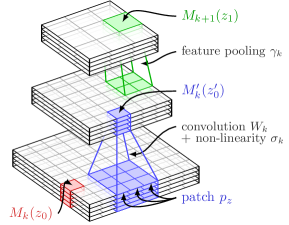
where $x$ is an input patch represented as a vector, the $W_{k}$’s are matrices corresponding to linear operations, the $\sigma_{k}$’s are pointwise non-linear functions, e.g., sigmoids or rectified linear units, and the functions $\gamma_{k}$ perform a downsampling operation called “feature pooling”. Each composition $\gamma_{k}(\sigma_{k}(W_{k}\bullet))$ is called a “layer” and the intermediate representations of $x$, between each layer, are called “maps”. A map can be represented as pixels organized on a spatial grid, with a multidimensional representation for each pixel. Borrowing a classical terminology from neuroscience, it is also common to call “receptive field” the set of pixels from the input patch $x$ that may influence a particular pixel value from a higher-layer map. In traditional convolutional neural networks, the $W_{k}$ matrices have a particular structure corresponding to spatial convolutions performed by small square filters, which will need to be learned. In the case where there is no such structure, the layer is called “fully-connected”.

The hyper-parameters of a convolutional architecture lie in the choice of non-linearities $\sigma_{k}$, type of pooling $\gamma_{k}$, in the structure of the matrices $W_{k}$ (notably the size and number of filters) as well as in the number of layers.

The only parameters that are learned in an automated fashion are usually the filters, corresponding to the entries of the matrices $W_{k}$. In this paper we investigate the following ways of learning: (i) encoding local descriptors with a CNN that has been trained for an unrelated classification task (Sec. 3.2.1), (ii) using a CNN that has been trained for a classification problem that can be directly linked to the target task (e.g. buildings, see Sec. 3.2.1), (iii) devising a surrogate classification problem to enforce invariance (Sec. 3.2.2), (iv) directly learning the weights using patch-level groundtruth (Sec. 3.3) or (v) using unsupervised learning, such as convolutional kernel networks, which we present in Section 4.

3.2 Learning Supervised Convolutional Descriptors

The traditional way of learning the weights ${\mathcal{W}=(W_{1},W_{2},\dots,W_{K})}$ in (1) consists in using a training set ${\mathcal{X}=(x_{1},x_{2},\dots,x_{n})}$ of examples, equipped with labels ${\mathcal{Y}=(y_{1},y_{2},\dots,y_{n})}$, choose a loss function ${\ell(\mathcal{X},\mathcal{Y},\mathcal{W})}$ and minimize it over $\mathcal{W}$ using stochastic gradient optimization and back-propagation (LeCun et al, 1989; Bottou, 2012). The choice of examples, labelings and loss functional leads to different weights.

Figure 2: Typical organization of two successive layers of a CNN. The spatial map $M^{\prime}_{k}$ is obtained from $M_{k}$ by convolution and pointwise non-linearity, and the top layer $M_{k+1}$ is obtained from $M^{\prime}_{k}$ by a downsampling operation called feature pooling. Usual CNNs use ReLU non-linearities and max-pooling (Krizhevsky et al, 2012), while CKNs rely on exponentials and Gaussian pooling (Mairal et al, 2014b).

3.2.1 Learning with category labels

A now classical CNN architecture is AlexNet (Krizhevsky et al, 2012). AlexNet consists of 8 layers: the first five are convolutional layers and the last ones are fully connected.

In this case, the training examples are images that have been hand-labeled into $C$ classes such as “bird” or “cow” and the loss function is the softmax loss:

$$\ell(\mathcal{X},\mathcal{Y},\mathcal{W})=\sum_{i=1}^{n}\log\sum_{j=1}^{C}\exp\left(M_{K}^{(i)}[j]-M_{K}^{(i)}[y_{i}]\right).$$ (2)

In Eq. (2) and throughout the paper, $M_{k}^{(i)}$ is the output of the $k$-th layer ($k\in\{1,\dots,K\}$) of the network applied to example $x_{i}$. The $[j]$ notation corresponds to the $j$-th element of the map.

Even though the network is designed to process images of size $224\times 224$, each neuron of a map has a “receptive field”, see the “coverage” column in Table 2 from Section 6. Using an image of the size of the receptive field produces a 1x1 map that we can use as a low dimensional patch descriptor. To ensure a fair comparison between all approaches, we rescale the fixed-size input patches so that they fit the required input of each network.

We explore two different sets of labellings for AlexNet: the first one, which we call AlexNet-ImageNet, is learned on the training set of ILSVRC 2012 ($C=1000$), as in the original paper (Krizhevsky et al, 2012). This set of weights is popular in off-the-shelf convolutional features, even though the initial task is unrelated to the target image retrieval application. Following Babenko et al (2014), we also fine-tune the same network on the Landmarks dataset, to introduce semantic information into the network that is more related to the target task. The resulting network is called AlexNet-Landmarks.

3.2.2 Learning from surrogate labels

Most CNNs such as AlexNet augment the dataset with jittered versions of training data to learn the filters $W_{k}$ in (1). Dosovitskiy et al (2014); Fischer et al (2014) use virtual patches, obtained as transformations of randomly extracted ones to design a classification problem related to patch retrieval. For a set of patches $\mathcal{P}$, and a set a transformations $\mathcal{T}$, the dataset consists of all $\tau(p),~{}(\tau,p)\in\mathcal{T}\times\mathcal{P}$. Transformed versions of the same patch share the same label, thus defining surrogate classes. Similarily to the previous setup, the network use softmax loss (2).

In this paper, we evaluate this strategy by using the same network, called PhilippNet, as in Fischer et al (2014). The network has three convolutional and one fully connected layers, takes as input 64x64 patches, and produces a 512-dimensional output.

3.3 Learning with patch-level groundtruth

When patch-level labels are available, obtained by manual annotation or 3D-reconstruction (Winder et al, 2009), it is possible to directly learn a similarity measure as well as a feature representation. The simplest way to do so, is to replace the virtual patches in the architecture of Dosovitskiy et al (2014); Fischer et al (2014) described in the previous section with labeled patches of RomeTrain. We call this version “FisherNet-Rome”.

It can also be achieved using a Siamese network (Chopra et al, 2005), i.e. a CNN which takes as input the two patches to compare, and where the objective function enforces that the output descriptors’ similarity should reproduce the ground-truth similarity between patches.

Optimization can be conducted with either a metric-learning cost (Simo-Serra et al, 2015):

$$\ell(\mathcal{X},\mathcal{Y},W_{K})=\sum_{i=1}^{n}\sum_{j=1}^{n}C(i,j,\|M^{(i)}_{K}-M^{(j)}_{K}\|)$$ (3)

with

$$C(i,j,d)=\left\{\begin{array}[]{ll}d&\mathrm{if}~{}y_{i}=y_{j}\\ \max(0,1-d)&\mathrm{otherwise}\end{array}\right.$$ (4)

or as a binary classification problem (“match”/“not-match”) with a softmax loss as in eq. (2) (Zbontar and LeCun, 2015; Zagoruyko and Komodakis, 2015). For those experiments, we use the parameters of the siamese networks of Zagoruyko and Komodakis (2015), available online. Following their convention, we refer to these architectures as “DeepCompare”.

4 Convolutional Kernel Networks

In this paper, the unsupervised learning strategy for learning convolutional networks is based on the convolutional kernel networks (CKNs) of Mairal et al (2014b). Similar to CNNs, these networks have a multi-layer structure with convolutional pooling and nonlinear operations at every layer. Instead of learning filters by optimizing a loss function, say for classification, they are trained layerwise to approximate a particular nonlinear kernel, and therefore require no labeled data.

The presentation of CKNs is divided into three stages: (i) introduction of the abstract model based on kernels (Sections 4.1, 4.2, and 4.3); (ii) approximation scheme and concrete implementation (Sections 4.4, 4.5, and 4.7); (iii) optimization (Section 4.6).

4.1 A Single-Layer Convolutional Kernel for Images

The basic component of CKNs is a match kernel that encodes a similarity between a pair of images $(M,M^{\prime})$ of size $m\times m\times d$ pixels, which are assumed to be square. The integer $d$ represents the number of channels, say 3 for RGB images. Note that when applied to image retrieval, these images $M,M^{\prime}$ correspond to regions – patches – extracted from an image. We omit this fact for simplicity since this presentation of CKNs is independent of the image retrieval task.

We denote by $\Omega$ the set of pixel locations, which is of size $|\Omega|=m\times m$, and choose a patch size $e\times e$. Then, we denote by $P_{z}$ (resp. $P^{\prime}_{z^{\prime}}$) the $e\times e\times d$ patch of $M$ (resp. $M^{\prime}$) at location $z\in\Omega$ (resp. $z^{\prime}\in\Omega$). Then, the single-layer match kernel is defined as follows:

Definition 1

Single-Layer Convolutional Kernel.

$$K(M,M^{\prime})=\sum_{z,z^{\prime}\in\Omega}e^{-\frac{1}{2\beta^{2}}\|z-z^{\prime}\|^{2}}\kappa(P_{z},P^{\prime}_{z^{\prime}}),$$ (5)

with

$$\kappa(P,P^{\prime})=\|P\|\|P^{\prime}\|e^{-\frac{1}{2\alpha^{2}}\|\tilde{P}-\tilde{P}^{\prime}\|^{2}},$$ (6)

where $\alpha$ and $\beta$ are two kernel hyperparameters, ${\|\cdot\|}$ denotes the usual $\ell_{2}$ norm, and $\tilde{P}$ and $\tilde{P}^{\prime}$ are $\ell_{2}$-normalized versions of the patches $P$ and $P^{\prime}$.

$K$ is called a convolutional kernel; it can be interpreted as a match-kernel that compares all pairs of patches from $M$ and $M^{\prime}$ with a nonlinear kernel $\kappa$, weighted by a Gaussian term that decreases with their relative distance. The kernel compares indeed all locations in $M$ with all locations in $M^{\prime}$. It depends notably on the parameter $\alpha$, which controls the nonlinearity of the Gaussian kernel comparing two normalized patches $\tilde{P}$ and $\tilde{P}^{\prime}$, and on $\beta$, which controls the size of the neighborhood in which a patch is matched with another one. In practice, the comparison of two patches that have very different locations $z$ and $z^{\prime}$ will be negligible in the sum (5) when $\beta$ is small enough. Hence, the parameter $\beta$ allows us to control the local shift-invariance of the kernel.

4.2 From Kernels to Infinite-Dimensional Feature Maps

Designing a positive definite kernel on data is equivalent to defining a mapping of the data to a Hilbert space, called reproducing kernel Hilbert space (RKHS), where the kernel is an inner product (Cucker and Zhou, 2007); exploiting this mapping is sometimes referred to as the “kernel trick” (Schölkopf and Smola, 2002). In this section, we will show how the kernel (5) may be used to generalize the concept of “feature maps” from the traditional neural network literature to kernels and Hilbert spaces. The kernel $K$ is indeed positive definite (see the appendix of Mairal et al 2014b) and thus it will suits our needs.

Basically, feature maps from convolutional neural networks are spatial maps where every location carries a finite-dimensional vector representing information from a local neighborhood in the input image. Generalizing this concept in an infinite-dimensional context is relatively straightforward with the following definition:

Definition 2

Let $\mathcal{H}$ be a Hilbert space. The set of feature maps is the set of applications $\varphi:\Omega\rightarrow\mathcal{H}$.

Given an image $M$, it is now easy to build such a feature map. For instance, consider the nonlinear kernel for patches $\kappa$ defined in Eq. (6). According to the Aronzsjan theorem, there exists a Hilbert space $\mathcal{H_{\kappa}}$ and a mapping $\phi_{\kappa}$ such that for two image patches $P,P^{\prime}$ – which may come from different images or not –, $\kappa(P,P^{\prime})=\langle\phi_{\kappa}(P),\phi_{\kappa}(P^{\prime})\rangle_{\mathcal{H}_{\kappa}}$. As a result, we may use this mapping to define a feature map $\varphi_{M}:\Omega\to{\mathcal{H}}_{\kappa}$ for image $M$ such that $\varphi_{M}(z)=\phi_{\kappa}(P_{z})$, where $P_{z}$ is the patch from $M$ centered at location $z$. The first property of feature maps from classical CNNs would be satisfied: at every location, the map carries information from a local neighborhood from the input image $M$.

We will see in the next subsection how to build sequences of feature maps in a multilayer fashion, with invariant properties that are missing from the simple example we have just described.

4.3 From Single-Layer to Multi-Layer Kernels

We now show how to build a sequence of feature maps $\varphi^{1}_{M}$, …, $\varphi^{k}_{M}$ for an input image $M$ initially represented as a finite-dimensional map $\varphi^{0}_{M}:\Omega_{0}\to{\mathbb{R}}^{p_{0}}$, where $\Omega_{0}$ is the set of pixel locations in $M$ and $p_{0}$ is the number of channels. The choice of initial map $\varphi_{M}^{0}$ is important since it will be the input of our algorithms; it is thus discussed in Section 4.7. Here, we assume that we have already made this choice, and we explain how to build a map $\varphi_{M}^{k}:\Omega_{k}\to{\mathcal{H}}_{k}$ from a previous map $\varphi_{M}^{{k\text{--}1}}:\Omega_{k\text{--}1}\to{\mathcal{H}}_{{k\text{--}1}}$. Specifically, our goal is to design $\varphi_{M}^{k}$ such that

• $\varphi_{M}^{k}(z)$ for $z$ in $\Omega_{k}$ carries information from a local neighborhood from $\varphi_{M}^{k\text{--}1}$ centered at location $z$;

• the map $\varphi_{M}^{k}$ is “more invariant” than $\varphi_{M}^{k\text{--}1}$.

These two properties can be obtained by defining a positive definite kernel $K_{k}$ on patches from $\varphi_{M}^{k\text{--}1}$. Denoting by ${\mathcal{H}}_{k}$ its RKHS, we may call $\varphi_{M}^{k}(z)$ the mapping to ${\mathcal{H}}_{k}$ of a patch from $\varphi_{M}^{{k\text{--}1}}$ centered at $z$. The construction is illustrated in Figure 3.

Figure 3: Construction of the sequence of feature maps $\varphi_{M}^{1},\ldots,\varphi_{M}^{k}$ for an input image $M$. The point $\varphi_{M}^{k}(z)$ for $z$ in $\Omega_{k}$ represents the mapping in ${\mathcal{H}}_{k}$ of a patch from $\varphi_{M}^{{k\text{--}1}}$ centered at $z$. Figure adapted from Mairal et al (2014b).

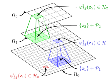
Concretely, we choose a patch shape ${\mathcal{P}}_{k}$, which is a set of coordinates centered at zero along with a set of pixel locations $\Omega_{k}$ such that for all $z$ in $\Omega_{k}$ and $u$ in ${\mathcal{P}}_{k}$, the location $z+u$ is in $\Omega_{{k\text{--}1}}$. Then, the kernel $K_{k}$ for comparing two patches from $\varphi_{M}^{k\text{--}1}$ and $\varphi_{M^{\prime}}^{k\text{--}1}$ at respective locations $z,z^{\prime}$ in $\Omega_{k}$ is defined as

$$\sum_{u,u^{\prime}\in{\mathcal{P}}_{k}}e^{-\frac{1}{2\beta_{k}^{2}}\|u-u^{\prime}\|^{2}}\kappa_{k}(\varphi_{M}^{k\text{--}1}(u+z),\varphi_{M}^{k\text{--}1}(u^{\prime}+z^{\prime})),$$ (7)

where

$$\kappa_{k}(\varphi,\varphi^{\prime})=\|\varphi\|_{{\mathcal{H}}_{k\text{--}1}}\|\varphi^{\prime}\|_{{\mathcal{H}}_{k\text{--}1}}e^{-\frac{1}{2\alpha_{k}^{2}}\|\tilde{\varphi}-\tilde{\varphi}^{\prime}\|^{2}_{{\mathcal{H}}_{k\text{--}1}}},$$

for all $\varphi,\varphi^{\prime}$ in ${\mathcal{H}}_{{k\text{--}1}}$, where $\tilde{\varphi}$ (resp. $\tilde{\varphi}^{\prime}$) are normalized—that is, $\tilde{\varphi}=(1/\|\varphi\|_{{\mathcal{H}}_{k\text{--}1}})\varphi$ if $\varphi=0$ and $0$ otherwise. This kernel is similar to the convolutional kernel for images already introduced in (5), except that it operates on infinite-dimensional feature maps. It involves two parameters $\alpha_{k}$, $\beta_{k}$ to control the amount of invariance of the kernel. Then, by definition, $\varphi_{M}^{k}:\Omega_{k}\to{\mathcal{H}}_{k}$ is the mapping such that the value (7) is equal to the inner product $\langle\varphi_{M}^{k}(z),\varphi_{M^{\prime}}^{k}(z^{\prime})\rangle_{{\mathcal{H}}_{k}}$.

This framework yields a sequence of infinite-dimensional image representations but requires finite-dimensional approximations to be used in practice. Among different approximate kernel embeddings techniques (Williams and Seeger, 2001; Bach and Jordan, 2002; Rahimi and Recht, 2008; Perronnin et al, 2010; Vedaldi and Zisserman, 2012), we will introduce a data-driven approach that exploits a simple expansion of the Gaussian kernel, and which provides a new way of learning convolutional neural networks without supervision.

4.4 Approximation of the Gaussian Kernel

Specifically, the previous approach relies on an approximation scheme for the Gaussian kernel, which is plugged in the convolutional kernels (7) at every layer; this scheme requires learning some weights that will be interpreted as the parameters of a CNN in the final pipeline (see Section 4.5).

More precisely, for all ${x}$ and ${x^{\prime}}$ in ${\mathbb{R}}^{q}$, and $\alpha>0$, the Gaussian kernel $e^{-\frac{1}{2\alpha^{2}}\|{x}-{x^{\prime}}\|_{2}^{2}}$ can be shown to be equal to

$$\left(\frac{2}{\pi\alpha^{2}}\right)^{\frac{q}{2}}\int_{{v}\in{\mathbb{R}}^{q}}e^{-\frac{1}{\alpha^{2}}\|{x}-{v}\|_{2}^{2}}e^{-\frac{1}{\alpha^{2}}\|{x^{\prime}}-{v}\|_{2}^{2}}d{v}.$$ (8)

Furthermore, when the vectors ${x}$ and ${x}^{\prime}$ are on the sphere—that is, have unit $\ell_{2}$-norm, we also have

$$e^{-\frac{1}{2\alpha^{2}}\|{x}-{x^{\prime}}\|_{2}^{2}}={\mathbb{E}}_{{v}\sim p({v})}[s({v}^{\top}{x})s({v}^{\top}{x^{\prime}})],$$ (9)

where $s$ is a nonlinear function such that $s(u)\propto e^{-\frac{1}{\alpha^{2}}+\frac{2u}{\alpha^{2}}}$ and $p({v})$ is the density of the multivariate normal distribution ${\mathcal{N}}(0,(\alpha^{2}/4){\mathbf{I}})$. Then, different strategies may be used to approximate the expectation by a finite weighted sum:

$$e^{-\frac{1}{2\alpha^{2}}\|{x}-{x^{\prime}}\|_{2}^{2}}\approx\frac{1}{p}\sum_{j=1}^{p}\eta_{j}s({v}_{j}^{\top}{x})s({v}_{j}^{\top}{x^{\prime}}),$$ (10)

which can be further simplified, after appropriate changes of variables,

$$e^{-\frac{1}{2\alpha^{2}}\|{x}-{x^{\prime}}\|_{2}^{2}}\approx\sum_{j=1}^{p}e^{{w}_{j}^{\top}{x}+b_{j}}e^{{w}_{j}^{\top}{x^{\prime}}+b_{j}},$$ (11)

for some sets of parameters ${w}_{j}$ in ${\mathbb{R}}^{p}$ and $b_{j}$ in ${\mathbb{R}}$, $j=1,\ldots,p$, which need to be learned. The approximation leads to the kernel approximations $\langle\psi({x}),\psi({x^{\prime}})\rangle$ where $\psi({x})=[e^{{w}_{j}^{\top}{x}+b_{j}}]_{j=1}^{p}$, which may be interpreted as the output of a one-layer neural network with $p$ neurons and exponential nonlinear functions.

The change of variable that we have introduced yields a simpler formulation than the original formulation of Mairal et al (2014b). Given a set of training pairs of normalized signals $({x}_{1},{x}_{1}^{\prime}),\ldots,({x}_{n},{x}_{n}^{\prime})$ in ${\mathbb{R}}^{q}$, the weights ${w}_{j}$ and scalars $b_{j}$ may now be obtained by minimizing

$$\min_{W,b}\quad\sum_{i=1}^{n}\left[e^{\frac{\|x_{i}-x^{\prime}_{i}\|^{2}}{2\alpha^{2}}}-\sum_{j=1}^{p}e^{w_{j}^{\top}x_{i}+b_{j}}e^{w_{j}^{\top}x^{\prime}_{i}+b_{j}}\right]^{2},$$ (12)

which is a non-convex optimization problem. How we address it will be detailed in Section 4.6.

4.5 Back to Finite-Dimensional Feature Maps

Convolutional kernel networks use the previous approximation scheme of the Gaussian kernel to build finite-dimensional image representations $M_{1}:\Omega_{1}\to{\mathbb{R}}^{p_{1}},M_{2}:\Omega_{2}\to{\mathbb{R}}^{p_{2}},\ldots,M_{k}:\Omega_{k}\to{\mathbb{R}}^{p_{k}}$ of an input image $M$ with the following properties:

• There exists a patch size $e_{k}\times e_{k}$ such that a patch $P_{l,z}$ of $M_{l}$ at location $z$—which is formally a vector of size $e_{k}^{2}p_{{k\text{--}1}}$—provides a finite-dimensional approximation of the kernel map $\varphi_{M}^{l}(z)$. In other words, given another patch $P^{\prime}_{l,z^{\prime}}$ from a map $M^{\prime}_{l}$, we have $\langle\varphi_{M}^{l}(z),\varphi_{M}^{l}(z)\rangle_{{\mathcal{H}}_{l}}\approx\langle P_{l,z},P^{\prime}_{l,z^{\prime}}\rangle$.

• Computing a map $M_{l}$ from $M_{{l\text{--}1}}$ involves convolution with learned filters and linear feature pooling with Gaussian weights.

Specifically, the learning and encoding algorithms are presented in Algorithms 1 and 2, respectively. The resulting procedure is relatively simple and admits two interpretations.

• The first one is to consider CKNs as an approximation of the infinite-dimensional feature maps $\varphi_{M}^{1},\ldots,\varphi_{M}^{k}$ presented in the previous sections (see Mairal et al, 2014b, for more details about the approximation principles).

• The second one is to see CKNs as particular types of convolutional neural networks with contrast-normalization. Unlike traditional CNNs, filters and nonlinearities are learned to approximate the Gaussian kernel on patches from layer ${k\text{--}1}$.

With both interpretations, this representation induces a change of paradigm in unsupervised learning with neural networks, where the network is not trained to reconstruct input signals, but where its non-linearities are derived from a kernel point of view.

Hyper-parameters: Kernel parameter $\alpha_{k}$, patch size $e_{k}\times e_{k}$, number of filters $p_{k}$.

Input model: A CKN trained up to layer ${k\text{--}1}$.

Input data: A set of training images.

Algorithm:

• Encode the input images using the CKN up to layer ${k\text{--}1}$ by using Algorithm 2;

• Extract randomly $n$ pairs of patches $(P_{i},P^{\prime}_{i})$ from the maps obtained at layer ${k\text{--}1}$;

• Normalize the patches to make then unit-norm;

• Learn the model parameters by minimizing (12), with $(x_{i},x_{i}^{\prime})=(P_{i},P_{i}^{\prime})$ for all $i=1,\ldots,n$;

Output: Weight matrix $W_{k}$ in ${\mathbb{R}}^{p_{{k\text{--}1}}e_{k}^{2}\times p_{k}}$ and $b_{k}$ in ${\mathbb{R}}^{p_{k}}$.

Algorithm 1 Training layer $k$ of a CKN.

Hyper-parameters: Kernel parameter $\beta_{k}$;

Input model: CKN parameters learned from layer $1$ to $k$ by using Algorithm 1;

Input data: A map $M_{k\text{--}1}:\Omega_{k-1}\to{\mathbb{R}}^{p_{{k\text{--}1}}}$;

Algorithm:

• Extract patches $\{P_{k,z}\}_{z\in\Omega_{{k\text{--}1}}}$ of size $e_{k}\times e_{k}$ from the input map $M_{k\text{--}1}$;

• Compute contrast-normalized patches

  $$\tilde{P}_{k,z}=\frac{1}{\|P_{k,z}\|}P_{k,z}~{}~{}\text{if}~{}~{}P_{k,z}\neq 0~{}~{}~{}\text{and}~{}~{}0~{}~{}\text{otherwise}.$$

• Produce an intermediate map $\tilde{M}_{k}:\Omega_{{k\text{--}1}}\to{\mathbb{R}}^{p_{k}}$ with linear operations followed by non-linearity:

  $$\tilde{M}_{k}(z)=\|P_{k,z}\|e^{W_{k}^{\top}\tilde{P}_{k,z}+b_{k}},$$ (13)

  where the exponential function is meant “pointwise”.

• Produce the output map $M_{k}$ by linear pooling with Gaussian weights:

  $$M_{k}(z)=\sum_{u\in\Omega_{{k\text{--}1}}}e^{-\frac{1}{\beta_{k}^{2}}\|u-z\|^{2}}\tilde{M}_{k}(u).$$

Output: A map $M_{k}:\Omega_{k}\to{\mathbb{R}}^{p_{k}}$ .

Algorithm 2 Encoding layer $k$ of a CKN.

4.6 Large-Scale Optimization

One of the challenge we faced to apply CKNs to image retrieval was the lack of scalability of the original model introduced by Mairal et al (2014b), which was a proof of concept with no effort towards scalability. A first improvement we made was to simplify the original objective function with changes of variables, resulting in the formulation (12), leading to simpler and less expensive gradient computations.

The second improvement is to use stochastic optimization instead of the L-BFGS method used by Mairal et al (2014b). This allows us to train every layer by using a set of one million patches and conduct learning on all of their possible pairs, which is a regime where stochastic optimization is unavoidable. Unfortunately, applying stochastic gradient descent directly on (12) turned out to be very ineffective due to the poor conditioning of the optimization problem. One solution is to make another change of variable and optimize in a space where the input data is less correlated.

More precisely, we proceed by (i) adding an “intercept” (the constant value 1) to the vectors $x_{i}$ in ${\mathbb{R}}^{q}$, yielding vectors $\tilde{x}_{i}$ in ${\mathbb{R}}^{q+1}$; (ii) computing the resulting (uncentered) covariance matrix $G=\frac{1}{n}\sum_{i=1}^{n}\tilde{x}_{i}\tilde{x}_{i}^{\top}$; (iii) computing the eigenvalue decomposition of $G=U\Delta U^{\top}$, where $U$ is orthogonal and $\Delta$ is diagonal with non-negative eigenvalues; (iv) computing the preconditioning matrix $R=U(\Delta+\tau I)^{1/2}U^{\top}$, where $\tau$ is an offset that we choose to be the mean value of the eigenvalues. Then, the matrix $R$ may be used as a preconditioner since the covariance of the vectors $R\tilde{x}_{i}$ is close to identity. In fact, it is equal to the identity matrix when $\tau=0$ and $G$ is invertible. Then, problem (12) with preconditioning becomes

$$\min_{Z}\quad\sum_{i=1}^{n}\left[e^{\frac{\|x_{i}-x^{\prime}_{i}\|^{2}}{2\alpha^{2}}}-\sum_{j=1}^{p}e^{z_{j}^{\top}R\tilde{x}_{i}}e^{z_{j}^{\top}R\tilde{x}^{\prime}_{i}}\right]^{2},$$ (14)

obtained with the change of variable $[W^{\top},b^{\top}]=Z^{\top}R$. Optimizing with respect to $Z$ to obtain a solution $(W,b)$ turned out to be the key for fast convergence of the stochastic gradient optimization algorithm.

Note that our effort also consisted on implementing heuristics for automatically selecting the learning rate during optimization without requiring any manual tuning, following in part standard guidelines from Bottou (2012). More precisely, we select the initial learning rate in the following range: $\{1,2^{-1/2},2^{-1},\ldots,2^{-20}\}$, by performing 1K iterations with mini-batches of size $1000$ and choosing the one that gives the lowest objective, evaluated on a validation dataset. After choosing the learning rate, we keep monitoring the objective on a validation set every 1K iteration, and perform backtracking in case of divergence. The learning rate is also divided by $\sqrt{2}$ every 50K iterations. The total number of iterations is set to 300K. Regarding initialization, weights are randomly initialized according to a standard normal distribution. These heuristics are fixed over all experiments and resulted in a stable parameter-free learning procedure, which we will release in an open-source software package.

4.7 Different Types of CKNs with Different Inputs

We have not discussed yet the initial choice of the map $M_{0}$ for representing an image $M$. In this paper, we follow Mairal et al (2014b) and investigate three possible inputs:

1. CKN-raw: We use the raw RGB values. This captures the hue information, which is discriminant information for many application cases.

2. CKN-white: It is similar to CKN-raw with the following modification: each time a patch $P_{0,z}$ is extracted from $M_{0}$, it is first centered (we remove its mean color), and whitened by computing a PCA on the set of patches from $M_{0}$. The resulting patches are invariant to the mean color of the original patch and mostly respond to local color variations.

3. CKN-grad: The input $M_{0}$ simply carries the two-dimensional image gradient computed on graysale values. The map has two channels, corresponding to the gradient computed along the x-direction and along the y-direction, respectively. These gradients are typically computed by finite differences.

Note that the first layer of CKN-grad typically uses patches of size $1\times 1$, which are in ${\mathbb{R}}^{2}$, and which are encoded by the first layer into $p_{1}$ channels, typically with $p_{1}$ in $[8;16]$. This setting corresponds exactly to the kernel descriptors introduced by Bo et al (2010), who have proposed a simple approximation scheme that does not require any learning. Interestingly, the resulting representation is akin to SIFT descriptors.

Denoting by $(G_{x,z},G_{y,z})$ the gradient components of image $M$ at location $z$, the patch $P_{z}$ is simply the vector $[G_{x,z},G_{y,z}]$ in ${\mathbb{R}}^{2}$. Then, the norm $\|P_{z}\|_{2}$ can be interpreted as the gradient magnitude $\rho_{z}=\sqrt{G_{x,z}^{2}+G_{y,z}^{2}}$, and the normalized patch $\tilde{P}_{z}$ represents a local orientation. In fact, there exists $\theta_{z}$ such that $\tilde{P}_{z}=[\cos(\theta_{z}),\sin(\theta_{z})]$. Then, we may use the relation (8) to approximate the Gaussian kernel $\exp(-\|\tilde{P}_{z}-\tilde{P}^{\prime}_{z^{\prime}}\|^{2}/(2\alpha_{1}^{2}))$. We may now approximate the integral by sampling $p_{1}$ evenly distributed orientations $\theta_{j}=2j\pi/p_{1},\,\,:j\in\{1,\dots,p_{1}\}$, and we obtain, up to a constant scaling factor,

$$e^{-\frac{1}{2\alpha_{1}^{2}}\|\tilde{P}_{z}-\tilde{P}^{\prime}_{z^{\prime}}\|^{2}}\approx\sum_{j=1}^{p_{1}}e^{-\frac{1}{\alpha_{1}^{2}}\|\tilde{P}_{z}-P_{\theta_{j}}\|^{2}}e^{-\frac{1}{\alpha_{1}^{2}}\|\tilde{P}^{\prime}_{z^{\prime}}-P_{\theta_{j}}\|^{2}},$$ (15)

where $P_{\theta}=[\cos(\theta),\sin(\theta)]$. With such an approximation, the $j$-th entry of the map $\tilde{M}_{1}(z)$ from (13) should be replaced by

$$\rho_{z}e^{-\frac{1}{2\alpha_{1}^{2}}\left((\cos(\theta_{j})-\cos(\theta_{z}))^{2}+(\sin(\theta_{j})-\sin(\theta_{z}))^{2}\right)}.$$

This formulation can be interpreted as a soft-binning of gradient orientations in a “histogram” of size $p_{1}$ at every location $z$. To ensure an adequate distribution in each bin, we choose $\alpha_{1}=\big{(}(1-\cos\left(2\pi/d_{1}\right))^{2}+\sin\left(2\pi/d_{1}\right)^{2}\big{)}^{1/2}$. After the pooling stage, the representation becomes very close to SIFT descriptors.

A visualization of all input methods can be seen in figure 4. See (Mairal et al, 2014a) for more analysis of image preprocessing.

Figure 4: Vizualization of the possible CKN inputs: CKN-raw (left); input when subtracting the mean color of each patch (middle-left); CKN-white, similar to the previous but with whitening (middle-right) and CKN-grad (right). Patches were extracted with a size of 3x3; images are reconstructed by averaging the pixel values of the pre-processed patches (up to normalization to fit the 0-256 range). Best viewed in color on a computer screen.

5 Datasets

In this section, we give details on the standard datasets we use to evaluate our method, as well as the protocol we used to create our new dataset.

5.1 Standard datasets

We give details on the commonly used benchmarks for which we report results.

5.1.1 Patch retrieval

The dataset introduced in (Mikolajczyk et al, 2005) in now standard to benchmark patch retrieval methods. This dataset consists of a set of 8 scenes viewed under 6 different conditions, with increasing transformation strength. In contrast to (Winder et al, 2009; Zagoruyko and Komodakis, 2015) where only DoG patches are available, the Mikolajczyk et al (2005) dataset allows custom detectors. We extract regions with the Hessian-Affine detector and match the corresponding descriptors with Euclidean nearest-neighbor. A pair of ellipses is deemed to match if the projection of the first region using the ground-truth homography on the second ellipse overlaps by at least 50%. The performance is measured in terms of mean average precision (mAP).

5.1.2 Image retrieval

We selected three standard image retrieval benchmarks: Holidays, Oxford and the University of Kentucky Benchmark (UKB).

Holidays

The Holidays dataset (Jégou et al, 2008) contains 500 different scenes or objects, for which 1,491 views are available. 500 images serve as queries. Following common practice, in contrast to (Babenko et al, 2014) though, we use the unrotated version, which allows certain views to display a $90^{\circ}$ rotation with respect to their query. While this has a non-negligible impact on performance for dense representations (the authors of (Babenko et al, 2014) report a 3% global drop in mAP), this is of little consequence for our pipeline which uses rotation-invariant keypoints. External learned parameters, such as k-means clusters for VLAD and PCA-projection matrix are learned on a subset of random Flickr images. The standard metric is mAP.

Oxford

The Oxford dataset (Philbin et al, 2007) consists of 5,000 images of Oxford landmarks. 11 locations of the city are selected as queries and 5 views per location is available. The standard benchmarking protocol, which we use, involves cropping the bounding-box of the region of interest in the query view, followed by retrieval. Some works, such as (Babenko et al, 2014) forgo the last step. Such a non-standard protocol yields a boost in performance. For instance Babenko and Lempitsky (2015) report a close to 6% improvement with non-cropped queries. mAP is the standard measure.

UKB

Containing 10,200 photos, the University of Kentucky Benchmark (UKB) (Nister and Stewenius, 2006) consists of 4 different views of the same object, under radical viewpoint changes. All images are used as queries in turn, and the standard measure is the mean number of true positives returned in the four first retrieved images ($4\times$recall@$4$).

5.2 Rome

One of the goals of this work is to establish a link between performance in patch retrieval with performance in image retrieval. Because of the way datasets are constructed differs (e.g. Internet-crawled images vs successive shots with the same camera, range of viewpoint changes, semantic content of the dataset, type of keypoint detector), patch descriptors may display different performances on different datasets. We therefore want a dataset that contains a groundtruth both at patch and image level, to jointly benchmark the two performances. Inspired by the seminal work of (Winder et al, 2009), we introduce the Rome retrieval dataset, based on 3D reconstruction of landmarks. The Rome16K dataset (Li et al, 2010) is a Community-Photo-Collection dataset that consists of 16,179 images downloaded from photo sharing sites, under the search term “Rome”. Images are partitioned into 66 “bundles”, each one containing a set of viewpoints of a given location in Rome (e.g. “Trevi Fountain”). Within a bundle, consistent parameters were automatically computed and are available. The set of 3D points that were reconstructed is also available, but we choose not to use them in favor of our Hessian-Affine keypoints. To determine matching points among images of a same bundle, we use the following procedure. i) we extract Hessian-Affine points in all images. For each pair of images of a bundle, we match the corresponding SIFTs, using Lowe’s reverse neighbor rule, as well as product quantization (Jégou et al, 2011) for speed-up. We filter matches, keeping those that satisfy the epipolar constraint up to a tolerance of $3$ pixels. Pairwise point matches are then greedily aggregated to form larger groups of 2D points viewed from several cameras. Groups are merged only if the reproduction error from the estimated 3D position is below the $3$ pixel threshold.

To allow safe parameter tuning, we split the set of bundles into a train and a test set, respectively containing 44 and 22 bundles.

5.2.1 Patch retrieval

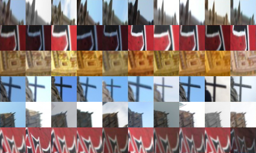
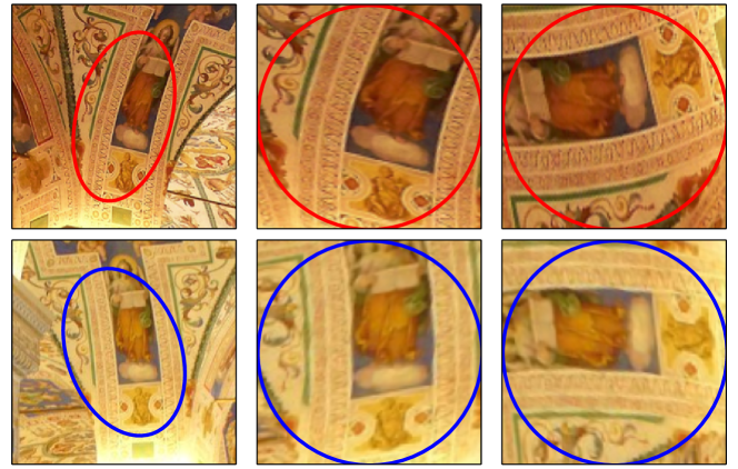
We design our patch retrieval datasets by randomly sampling in each train and test split a set of $1,000$ 3D points for which at least $10$ views are available. The sampling is uniform in the bundles, which means that we take roughly the same amount of 3D points from each bundle. We then sample $10$ views for each point, use one as a query and the remaining as targets. Both our datasets therefore contain $1,000$ queries and $9,000$ retrieved elements. We report mean average precision (mAP). An example of patch retrieval classes can be seen in Fig. 5.

Figure 5: Examples of patches matched under our procedure. We observe significant changes in lighting, but smaller changes in rotation and skew.

5.2.2 Image retrieval

Using the same aforementioned train-test bundle split, we select 1,000 query images and 1,000 target images evenly distributed over all bundles. Two images are deemed to match if they come from the same bundle, as illustrated in Fig. 6

Figure 6: Example of classes of the image retrieval dataset of Rome. Each class consists of a particular location. Some bundle display significant viewpoint changes (extreme left and right), while others have little variation in appearance (middle). Best viewed in color.

6 Experiments

In this section, we describe the implementation of our pipelines, and report results on patch and image retrieval benchmarks.

6.1 Implementation details

We provide details on the patch and image retrieval pipelines. Our goal is to evaluate the performance of patch descriptors, and all methods are therefore given the same input patches (computed at Hessian-Affine keypoints), possibly resized to fit the required input size of the method. We also evaluate all methods with the same aggregation procedure (VLAD with 256 centroids). We believe that improvements in feature detection and aggregation are orthogonal to our contribution and would equally benefit all architectures.

6.1.1 Pipeline

We briefly review our image retrieval pipeline.

Keypoint detection.

Figure 7: Example of matching points in two different images. Salient points are extracted (left), affine rectified (middle), and normalized in rotation (right). Note that the level of invariance which remains to be covered by the patch descriptor is relatively low, as most of the work has been accomplished by the detector.

A popular design choice in image representations, inspired by text categorization methods, is to consider images as sets of local patches, taken at various locations. The choice of these locations is left to the interest point detector, for which multiple alternatives are possible.

In this work, we use the popular “Hessian-Affine” detector of Mikolajczyk and Schmid (2004). It aims at finding reproducible points, meaning that selected 3D points of a scene should always belong to the set of detected image points when the camera undergoes small changes in settings (e.g. viewpoint, blur, lighting). Because of the “aperture” problem the set of such points is limited to textured patches, to the exclusion of straight lines, for which precise localization is impossible. This leaves “blobs”, as used for instance in Lowe’s Difference of Gaussians (DoG) detector (Lowe, 2004) or corners, as is the case for our Hessian-Affine detector. Specifically, a “cornerness” measure is computed on the whole image, based on the Hessian of the pixel intensities. The set of points whose cornerness is above a threshold is kept. The detector takes the points at their characteristic scale and estimates an affine-invariant local region. Rotation invariance is achieved by ensuring the dominant gradient orientation always lies in a given direction. This results in a set of keypoints with locally-affine invariant regions. Fig. 7 shows the various steps for detecting keypoints. We sample the point with a resolution of $51\times 51$ pixels, value that was found optimal for SIFT on Oxford. Pixels that fall out of the image are set to their nearest neighbor in the image. This strategy greatly increases patch retrieval performance compared to setting them to black, as it does not introduce strong gradients.

Note that the choice of a particular interest point detector is arbitrary and our method is not specific to Hessian-Affine locations. To show this, we also experiment with dense patches in section 6.3.5

Patch description.

Because of the affine-invariant detectors, and as seen in Fig. 7, for a given 3D point seen in two different images, the resulting patches have small differences (e.g. lighting, blur, small rotation, skew). The goal of patch description, and the focus of this work, is to design a patch representation, i.e. a mapping $\Phi$ of the space of fixed-size patches into some Hilbert space, that is robust to these changes.

Matching/Aggregation.

Stereo-vision uses this keypoint representation to establish correspondences between images of the same instance, with 3D reconstruction as an objective. The cost of this operation is quadratic in the number of keypoints, which is prohibitive in image retrieval systems that need to scan through large databases. Instead, we choose to aggregate the local patch descriptors into a fixed-length global image descriptor. For this purpose, we use the popular VLAD representation (Jégou et al, 2012). Given a clustering in the form of a Voronoi diagram with points $\{c_{1},\dots,c_{k}\}$ of the feature space (typically obtained using k-means on an external set of points), VLAD encodes the set of visual words $\{x_{1},\dots,x_{n}\}$ as the total shift with respect to their assigned centroid:

$${\rm VLAD}=\sum_{i=1}^{k}\sum_{j=1}^{n}\varepsilon_{i,j}(x_{j}-c_{i}),$$ (16)

where $\varepsilon_{i,j}$ is the assignment operator, which is 1 if $x_{j}$ is closer to centroid $c_{i}$ than to the others, and 0 otherwise.

The final VLAD descriptors is power-normalized with exponent 0.5 (signed square-root), as well as $\ell_{2}$-normalized.

6.1.2 Convolutional Networks training

AlexNet-ImageNet.

We use the Caffe package (Jia et al, 2014) and its provided weights for AlexNet, that have been learned according to Krizhevsky et al (2012). Specifically, the network was trained on ILSVRC’12 data for 90 epochs, using a learning rate initialized to $10^{-2}$ and decreased three times prior to termination. Weight decay was fixed to 0.0005, momentum to 0.9 and dropout rate to 50%. It uses three types of image jittering: random $227\times 227$ out of $256\times 256$ cropping, flip and color variation.

AlexNet-Landmarks.

Following Babenko et al (2014), we fine-tune AlexNet using images of the Landmarks dataset. Following their protocol, we strip the network of its last layer and replace it with a 671-dim fully-connected one, initialized with random Gaussian noise (standard deviation 0.01). Other layers are initialized with the old AlexNet-ImageNet weights. We use a learning rate of $10^{-3}$ for fine-tuning. Weight decay, momentum and dropout rate are kept to their default values (0.0005, 0.9 and 0.5). We use data augmentation at training time, with the same transformations as in the original paper (crop, flip and color). We decrease the learning rate by 10 when it saturates (around 20 epochs each time). We report a validation accuracy of 59% on the Landmarks dataset, which was confirmed through discussion with the authors. On Holidays, we report a mAP of 77.5 for the sixth layer (against 79.3 in (Babenko et al, 2014)), and 53.6 (against 54.5) on Oxford. Even though slightly below the results in the original paper, fine-tuning still significantly improves on ImageNet weights for retrieval.

PhilippNet.

For PhilippNet, we used the model provided by the authors. The model is learned on 16K surrogate classes (randomly extracted patches) with 150 representatives (composite transformations, including crops, color and contrast variation, blur, flip, etc.). We were able to replicate their patch retrieval results on their dataset, as well as on Mikolajczyk et al’s dataset when using MSER keypoints.

PhilippNet-Rome.

The patch retrieval dataset of RomePatches does not contain enough patches to learn a deep network. We augment it using patches extracted in a similar fashion, grouped in classes that correspond to 3D locations and contain at least 10 examples. We build two such training sets, one with 10K classes, and one with 100K classes. Training is conducted with the default parameters.

Deepcompare.

As previously described, we use the online code provided by Zagoruyko and Komodakis (2015). It consists of networks trained on the three distinct datasets of Winder et al (2009): Liberty, NotreDame and Yosemity. For our image retrieval experiments, we can only use the siamese networks, as the others do not provide a patch representation. These were observed in the original paper to give suboptimal results.

Convolutional Kernel Networks

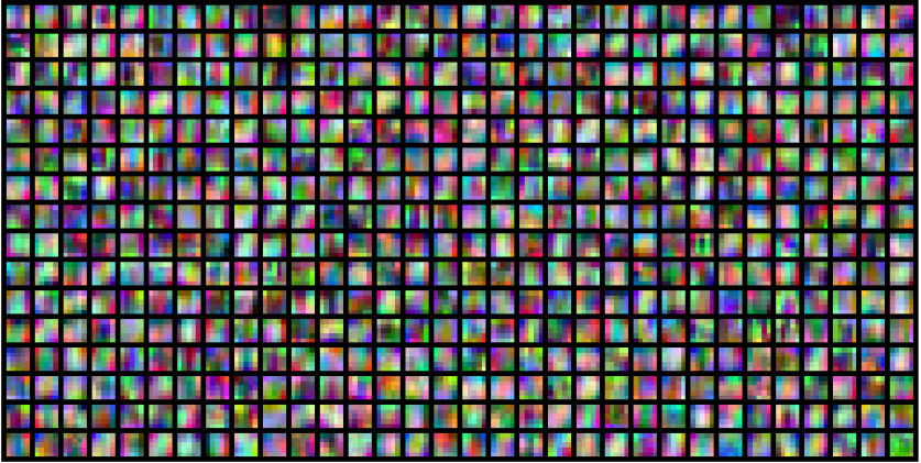
To train the convolutional kernel networks, we randomly subsample a set of 100K patches in the train split of the Rome dataset. For each layer, we further extract 1M sub-patches with the required size, and feed all possible pairs as input to the CKN. The stochastic gradient optimization is run for 300K iterations with a batch size of 1000, following the procedure described in section 4.6. Training a convolutional kernel network, for a particular set of hyperparameters, roughly takes 10 min on a GPU. This stands in contrast to the 2-3 days for training using the L-BFGS implementation used in Mairal et al (2014b). We show in Fig. 8 a visualization of the first convolutional filters of CKN-raw. The sub-patches for CKN-grad and CKN-white are too small ($3\times 3$) and not adapted to viewing.

Figure 8: All 512 kernels of the first layer of our CKN-raw architecture.

6.2 Patch retrieval

6.2.1 CKN parametric exploration

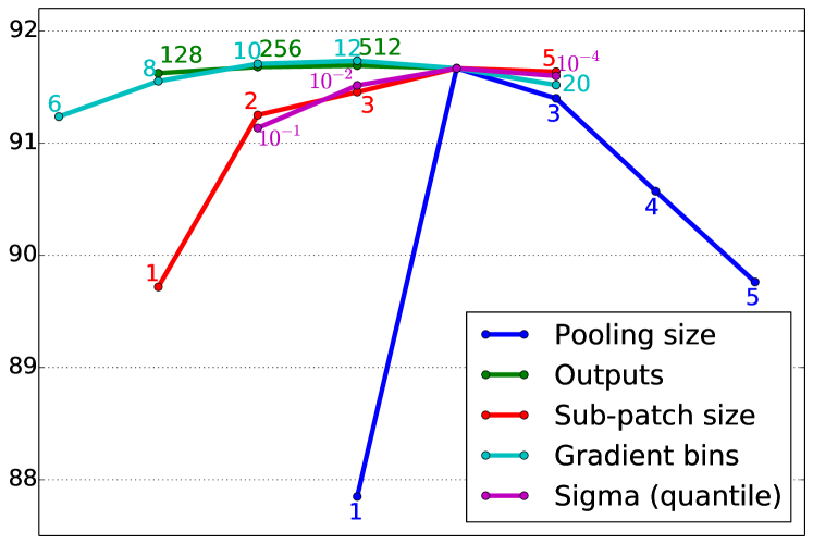
The relatively low training time of CKNs (10 min. on a recent GPU), as well as the fact that the training is layer-wise – and therefore lower layer parameters can be reused if only the top layer change – allows us to test a relatively high number of parameters, and select the ones that best suit our task. We tested parameters for convolution and pooling patch sizes in range of $2$ to $5$, number of neuron features in powers of $2$ from 128 to 1024. For the $\sigma$ parameter, the optimal value was found to be $10^{-3}$ for all architectures. For the other parameters, we keep one set of optimal values for each input type, described in Table 1.

Input	Layer 1	Layer 2	dim.
CKN-raw	5x5, 5, 512	—-	41,472
CKN-white	3x3, 3, 128	2x2, 2, 512	32,768
CKN-grad	1x1, 3, 16	4x4,2,1024	50,176

Table 1: For each layer we indicate the sub-patch size, the subsampling factor and the number of filters. For the gradient network, the value $16$ corresponds to the number of orientations.

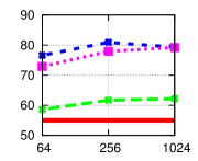
In Figure 9, we explore the impact of the various hyper-parameters of CKN-grad, by tuning one while keeping the others to their optimal values.

Figure 9: mAP results on the train set of RomePatches with CKN-grad, whose hyper-parameters have been changed one by one around the optimal point. Note that 10 and 12 gradient bins give slightly better results but 16 was kept to align with the logarithm scale of the grid.

6.2.2 Dimensionality reduction

Since the final dimension of the CKN descriptor is prohibitive for most applications of practical value (see Table 1), we investigate dimensionality reduction techniques. Note that this step is unnecessary for CNNs, whose feature dimension do not exceed 512 (PhilippNet). We only perform unsupervised dimensionality reduction through PCA, and investigate several forms of whitening. Denoting $X$ the $n\times d$ matrix of $n$ CKN features (we used $n=10K$), the singular value decomposition of $X$ writes as

$$X=USV^{\top},$$ (17)

where $U$ and $V$ are orthogonal matrices and $S$ is diagonal with non-increasing values from upper left to bottom right. For a new $n^{\prime}\times d$ matrix of observations $X^{\prime}$, the dimensionality reduction step writes as

$$X^{\prime}_{\rm proj}=XL^{\top},$$ (18)

where $L$ is a $d^{\prime}\times d$ projection matrix.

The three types of whitening we use are: i) no whitening; ii) full whitening; iii) semi-whitening. Full whitening corresponds to

$$L=V(1:d^{\prime},:)/D(1:d^{\prime},1:d^{\prime})\;,$$ (19)

while semi-whitening corresponds to

$$L=V(1:d^{\prime},:)/\sqrt{D(1:d^{\prime},1:d^{\prime})}\;.$$ (20)

The matrix division $/$ denotes the matrix multiplication with the inverse of the right-hand matrix. The square-root is performed element-wise.

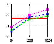
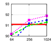
Results of the different methods on the RomePatches dataset are displayed in Fig. 10. We observe that semi-whitening works best for CKN-grad and CKN-white, while CKN-raw is slightly improved by full whitening. We keep these methods in the remainder of this article, as well as a final dimension of 1024.

CKN-grad	CKN-raw	CKN-white

Figure 10: Influence of dimensionality reduction on patch retrieval performance. Results reported in mAP (%) on the train split of RomePatches as a function of the PCA dimension. As a comparison, SIFT reports 91.6%.

6.2.3 Results

We compare the convolutional architectures on our three patch datasets: RomePatches-train, RomePatches-test and Mikolajczyk et al’s dataset. Results are given in Table 2. For AlexNet CNNs, we report results for all outputs of the 5 convolutional layers (after ReLU). We note that SIFT is an excellent baseline for these methods, and that CNN architectures that were designed for local invariances perform better than the ones used in AlexNet, as observed by Fischer et al (2014). The results of the PhilippNet on Mikolajczyk et al’s dataset are different from the ones reported by Fischer et al (2014), as we evaluate on Hessian-Affine descriptors while they use MSER. To have a comparable setting, we use their network with an input of 64x64 that corresponds to the coverage of one top neuron, as well as their protocol that slide it on 91x91 patches. We notice that this last step only provides a small increase of performance (2% for patch retrieval and 1% for image retrieval). We observe that PhilippNet outperforms both SIFT and AlexNet, which was the conclusion of Fischer et al (2014); CKN trained on whitened patches do however yield better results.

Architecture	coverage	Dim	RomePatches		Miko.
			train	test
SIFT	51x51	128	91.6	87.9	57.8
AlexNet-conv1	11x11	96	66.4	65.0	40.9
AlexNet-conv2	51x51	256	73.8	69.9	46.4
AlexNet-conv3	99x99	384	81.6	79.2	53.7
AlexNet-conv4	131x131	384	78.4	75.7	43.4
AlexNet-conv5	163x163	256	53.9	49.6	24.4
PhilippNet	64x64	512	86.1	81.4	59.7
PhilippNet	91x91	2048	88.0	83.7	61.3
CKN-grad	51x51	1024	92.5	88.1	59.5
CKN-raw	51x51	1024	79.3	76.3	50.9
CKN-white	51x51	1024	91.9	87.7	62.5

Table 2: Results of convolutional architectures for patch retrieval.

6.2.4 DeepCompare

As the architectures of DeepCompare (Zagoruyko and Komodakis, 2015) do not rely on an underlying patch descriptor representation but rather on similarities between pairs of patches, some architectures can only be tested for patch-retrieval. We give in Table 3 the performances of all their architectures on RomePatches.

Network	RomePatches-Train	RomePatches-Test
2ch2stream Y	89.3	85.7
2ch2stream ND	88.3	84.9
2ch2stream L	90.2	86.6
2ch Y	86.6	83.5
2ch ND	81.2	78.4
2ch L	83.4	80.1
siam Y	82.9	79.2
siam ND	84.8	81.0
siam L	83.2	79.8
siam2stream Y	78.8	75.4
siam2stream ND	84.2	80.6
siam2stream L	82.0	78.6

Table 3: Evaluation of the deepcompare architectures on RomePatches in mAP (%). Networks were trained on the three subsets of the Multi-view Stereo Correspondence Dataset: Yosemity (Y), Notre-Dame (ND) and Statue of Liberty (L). The network notations are as in the original paper (Zagoruyko and Komodakis, 2015).

We note that the only networks that produce descriptors that can be used for image retrieval are the architectures denoted “siam” here. They also perform quite poorly compared to the others. Even the best architectures are still below the SIFT baseline (91.6/87.9).

The method of Zagoruyko and Komodakis (2015) optimizes and tests on different patches (DoG points, 64x64 patches, greyscale), which explains the poor performances when transferring them to our RomePatches dataset. The common evaluation protocol on this dataset is to sample the same number of matching and non-matching pairs, rank them according to the measure and report the false positive rate at 95% recall (“FPR@95%”, the lower the better). The patches used for the benchmark are available online, but not the actual split used for testing. With our own split of the Liberty dataset, we get the results in Table 4. We note that all our results, although differing slightly from the ones of Zagoruyko and Komodakis (2015), do not change their conclusions.

Descriptor	FPR@95% (%)
SIFT	19.9
Best AlexNet (3)	13.5
siam-l2 (trained on Notre-Dame)	14.7
2ch-2stream (trained on Notre-Dame)	1.24
CKN-grad	27.7
CKN-white	30.4
CKN-raw	41.7
best CKN	14.4

Table 4: Experiments on a set of pairs of the Liberty dataset. Measure is false positive rate @95% recall, and therefore the lower the better. The third layer of AlexNet is used, as it provides the best results.

We note that our CKNs whose hyperparameters were optimized on RomePatches work poorly. However, optimizing again the parameters for CKN-grad on a grid leads to a result of 14.4% (“best CKN”). To obtain this result, the number of gradient histogram bins was reduced to 6, and the pooling patch size was increased to 8 on the first layer and 3 on the second. These changes indicate that the DoG keypoints are less invariant to small deformations, and therefore require less rigid descriptors (more pooling, less histograms). The results are on par with all comparable architectures (siam-l2: 14.7%, AlexNet: 13.5%), as the other architectures either use central-surround networks or methods that do not produce patch representations. The best method of Zagoruyko and Komodakis (2015), 2ch-2stream, reports an impressive 1.24% on our split. However, as already mentioned, this architecture does not produce a patch representation and it is therefore difficult to scale to large-scale patch and image retrieval applications.

6.2.5 Impact of supervision

We study the impact of the different supervised trainings, between surrogate classes and real ones. Results are given in Table 5.

Training parameters	RomePatches-Train	RomePatches-Test
PhilippNet	86.1	81.4
PhilippNet-Rome 10K	84.1	80.1
PhilippNet-Rome 100K	89.9	85.6
(Best) CKN-grad	92.5	88.1
(Baseline) SIFT	91.6	87.9

Table 5: Impact of supervision on patch retrieval. PhilippNet is trained on surrogate classes, while PhilippNet-Rome is trained on a larger set of RomePatches-Train, containing either 10K or 100K classes. We see that retraining improves performance provided enough data is given. Supervised CNNs are still below the SIFT baseline, as well as the unsupervised CKNs.

Figure 11: First convolutional filters of the PhilippNet learned with surrogate classes (left), 10K Rome classes (middle) and 100K Rome classes. Best viewed in color.

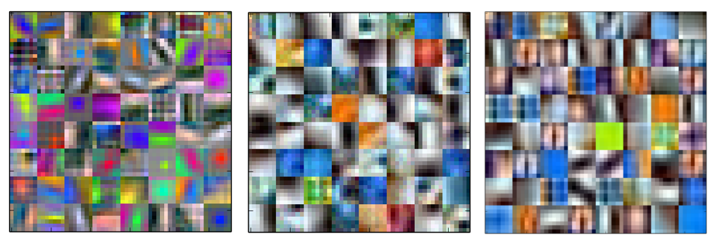
Figure 11 gives the first convolutional filters of the PhilippNet learned on surrogate classes, and on Rome. As can be seen, the plain surrogate version reacts to more diverse color, as it has been learned with diverse (ImageNet) input images. Both Rome 10K and Rome 100K datasets have colors that correspond to skies and buildings and focus more on gradients. It is interesting to note that the network trained with 100K classes seems to have captured finer levels of detail than its 10K counterpart.

6.2.6 Robustness

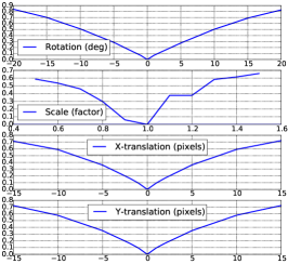
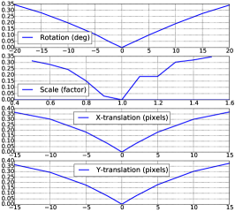
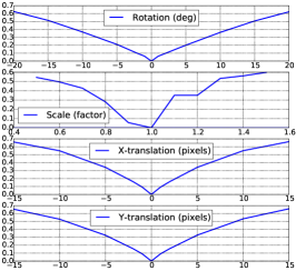
We investigate in Fig. 12 the robustness of CKN descriptors to transformations of the input patches, specifically rotations, zooms and translations. We select 100 different images, and extract the same patch by jittering the keypoint along the aforementioned transformation. We then plot the average $L_{2}$ distance between the descriptor of the original patch and the transformed one. Note the steps for the scale transformation; this is due to the fact that the keypoint scale is quantized on a scale of powers of 1.2, for performance reasons.

Figure 12: Impact of various transformations on CKN descriptors. Represented is the average distance between a patch descriptor and its jittered version, as a function of the transformation magnitude. Best viewed in numerical format.

6.3 Image retrieval

6.3.1 Settings.

We learn a vocabulary of $256$ centroids on a related database: for Holidays and UKB we use 5,000 Flickr images and for Oxford, we train on Paris (Philbin et al, 2008). The vocabulary for RomePatches-Train is learned on RomePatches-Test and vice-versa. The final VLAD descriptor size is 256 times the local descriptor dimension.

6.3.2 Results

We compare all convolutional approaches as well as the SIFT baseline in the image retrieval settings. Results are summarized in Table 6.

	Holidays	UKB	Oxford	Rome
				train	test
SIFT	64.0	3.44	43.7	52.9	62.7
AlexNet-conv1	59.0	3.33	18.8	28.9	36.8
AlexNet-conv2	62.7	3.19	12.5	36.1	21.0
AlexNet-conv3	79.3	3.74	33.3	47.1	54.7
AlexNet-conv4	77.1	3.73	34.3	47.9	55.4
AlexNet-conv5	75.3	3.69	33.4	45.7	53.1
PhilippNet 64x64	74.1	3.66	38.3	50.2	60.4
PhilippNet 91x91	74.7	3.67	43.6	51.4	61.3
CKN-grad	66.5	3.42	49.8	57.0	66.2
CKN-raw	69.9	3.54	23.0	33.0	43.8
CKN-white	78.7	3.74	41.8	51.9	62.4
CKN-mix	79.3	3.76	43.4	54.5	65.3

Table 6: Image retrieval results. Results are in mAP except for UKB where we measure the average number of true positives in the first 4 results. CKN-mix is the result of the concatenation of the VLAD descriptors for the three channels.

On datasets for which color is dominant (e.g. Holidays or UKB), the best individual CKN results are attained by CKN-white, improved by combining the three channels. On images of buildings, gradients still perform best and the addition of color channels is harmful, which explains on the one hand the poor performance of AlexNet and on the other hand the relatively good performance of PhilippNet which was explicitly trained to be invariant to colorimetric transformations.

6.3.3 Influence of context

Through experiments with AlexNet-landmarks, we study the impact of context in the local features. Specifically, we test whether fine-tuning on a dataset that shares semantic information with the target retrieval dataset improves performance. We compare the same network architecture – AlexNet – in two settings: when parameters are learned on ImageNet (which involves a varied set of classes) and when they are learned on the Landmarks dataset which solely consists of buildings and places. Results, shown in Table 7, show clear improvement for Oxford, but not for Holidays. We explain this behavior by the fact that the network learns building-specific invariances and that fewer building structures are present in Holidays as opposed to Oxford.

	Holidays		Oxford
	ImageNet	Landmarks	ImageNet	Landmarks
conv1	59.0	57.7	18.8	20.7
conv2	62.7	72.4	12.5	23.8
conv3	79.3	76.1	33.3	38.6
conv4	77.1	73.9	34.3	38.3
conv5	75.3	66.1	33.4	32.5

Table 7: Influence of the pretraining dataset on image retrieval. With the same architecture (AlexNet), training is conducted either on ILSVRC’12 data or on the Landmarks dataset. Using semantic information related to buildings and places yields improvements for Oxford, but not for Holidays.

6.3.4 Dimensionality reduction

As observed in previous work (Jégou and Chum, 2012), projecting the final VLAD descriptor to a lower dimension using PCA+whitening can lead to lower memory costs, and sometimes to slight increases in performance (e.g. on Holidays (Gong et al, 2014)). We project to 4096-dim descriptors, the same output dimension as  Babenko et al (2014) and obtain the results in Table 8. We indeed observe a small improvement on Holidays but a small decrease on Oxford.

Dataset	Holidays	UKB	Oxford
	(CKN-mix)	(CKN-mix)	(CKN-grad)
Full (262K-dim)	79.3	3.76	49.8
PCA (4096-dim)	82.9	3.77	47.2

Table 8: Impact of dimensionality reduction by PCA+whitening on the best channel for each dataset. PCA to 4096 dimensions.

6.3.5 Dense keypoints

Our choice of Hessian-Affine keypoints is arbitrary and can be suboptimal for some image retrieval datasets. Indeed we observe that by sampling points on a regular grid of $8\times 8$ pixels at multiple scales, we can improve results. We learn the CKN parameters and the PCA projection matrix on a dense set of points in Rome, and apply it to image retrieval as before. We use SIFT descriptors as a baseline, extracted at the exact same locations. We observe that for CKN-grad and CKN-white, the previous models lead to suboptimal results. However, increasing the pooling from 3 (resp. 2 for the second layer) to 4 (resp. 3), leads to superior performances. We attribute this to the fact that descriptors on dense points require more invariance than the ones computed at Hessian-Affine locations. Results on the Holidays dataset are given in Table 9. As observed on Hessian-Affine points, the gradient channel performs much better on Oxford. We therefore only evaluate this channel. As explained in section 5, there are two ways to evaluate the Oxford dataset. The first one crops queries, the second does not. While we only consider the first protocol to be valid, it is interesting to investigate the second, as results in Table 10 tend to indicate that it favors dense keypoints (and therefore the global descriptors of Babenko et al (2014)).

Descriptor	SIFT	grad	raw	white	mix
Hessian-Affine	64.0	66.5	69.9	78.7	79.3
Dense (same parameters)	70.3	68.5	72.3	76.8	.
Dense (changed pooling)	70.3	71.3	72.3	80.8	82.6

Table 9: Dense results on Holidays. Right hand side of the table are CKN descriptors. “Same parameters” correspond to CKNs that have the same parameters as Hessian-Affine ones, yet learned on densely extracted patches. “Changed pooling” have pooling size increased by one at each layer (CKN-raw is unchanged as it only has one layer, and already gives good performances).

Method $\backslash$ descriptor	SIFT	CKN-grad
Hessian-Affine, no crop	45.7	49.0
Hessian-Affine, crop	43.7	49.8
Dense, no crop	51.1	55.4
Dense, crop	47.6	50.9

Table 10: Dense keypoints on the Oxford dataset. “Crop” indicates the protocol where queries are cropped to a small bounding-box containing the relevant object, while “no crop” takes the full image as a query. For CKN, parameters have increased pooling sizes for dense keypoints, as on Holidays.

6.3.6 Comparison with state of the art

Table 11 compares our approach to recently published results. Approaches based on VLAD with SIFT (Arandjelovic and Zisserman, 2013; Jégou et al, 2012) can be improved significantly by CKN local descriptors (+15% on Holidays). To compare to the state of the art with SIFT on Oxford (Arandjelovic and Zisserman, 2013), we use the same Hessian-Affine patches extracted with gravity assumption (Perd’och et al, 2009). Note that this alone results in a $7\%$ gain.

We also compare with global CNN (Babenko et al, 2014). Our approach outperforms it on Oxford, UKB, and Holidays. For CNN features with sum-pooling encoding (Babenko and Lempitsky, 2015), we report better results on Holidays and UKB, and on Oxford with the same evaluation protocol. Note that their method works better than ours when used without cropping the queries (58.9%).

On Holidays, our approach is slightly below the one of Gong et al (2014), that uses AlexNet descriptors and VLAD pooling on large, densely extracted patches. It is however possible to improve on this result by using the same dimensionality reduction technique (PCA+whitening) which gives 82.9% or dense keypoints (82.6%).

Method $\backslash$ Dataset	Holidays	UKB	Oxford
VLAD (Jégou et al, 2012)	63.4	3.47	-
VLAD++ (Arandjelovic and Zisserman, 2013)	64.6	-	55.5*
Global-CNN (Babenko et al, 2014)	79.3	3.56	54.5
MOP-CNN (Gong et al, 2014)	80.2	-	-
Sum-pooling OxfordNet (Babenko and Lempitsky, 2015)	80.2	3.65	53.1
Ours	79.3 (82.9)	3.76	49.8 (56.5*)

Table 11: Comparison with state-of-the-art image retrieval results. Results with * use a Hessian-Affine detector with gravity assumption (Perd’och et al, 2009). Our best result on Holidays uses whitening as in MOP-CNN.

7 Conclusion

We showed that Convolutional Kernel Networks (CKNs) offer similar and sometimes even better performances than classical Convolution Neural Networks (CNNs) in the context of patch description, and that the good performances observed in patch retrieval translate into good performances for image retrieval, reaching state-of-the-art results on several standard benchmarks. The main advantage of CKNs compared to CNNs is their very fast training time, and the fact that unsupervised training suppresses the need for manually labeled examples. It is still unclear if their success is due to the particular level of invariance they induce, or their low training time which allows to efficiently search through the space of hyperparamaters. We leave this question open and hope to answer it in future work.

Acknowledgments. This work was partially supported by projects “Allegro” (ERC), “Titan” (CNRS-Mastodon), “Macaron” (ANR-14-CE23-0003-01), the Moore-Sloan Data Science Environment at NYU and a Xerox Research Center Europe collaboration contract. We wish to thank Fischer et al (2014); Babenko et al (2014); Gong et al (2014) for their helpful discussions and comments. We gratefully acknowledge the support of NVIDIA Corporation with the donation of the GPUs used for this research.

References

- Agrawal et al (2015) Agrawal P, Carreira J, Malik J (2015) Learning to see by moving. In: IEEE Conference on Computer Vision and Pattern Recognition
- Arandjelovic and Zisserman (2013) Arandjelovic R, Zisserman A (2013) All about VLAD. In: IEEE Conference on Computer Vision and Pattern Recognition
- Babenko and Lempitsky (2015) Babenko A, Lempitsky V (2015) Aggregating deep convolutional features for image retrieval. In: International Conference on Computer Vision
- Babenko et al (2014) Babenko A, Slesarev A, Chigorin A, Lempitsky V (2014) Neural codes for image retrieval. In: European Conference on Computer Vision
- Bach and Jordan (2002) Bach FR, Jordan MI (2002) Kernel independent component analysis. Journal of Machine Learning Research
- Bay et al (2006) Bay H, Tuytelaars T, Van Gool L (2006) SURF: Speeded up robust features. In: European Conference on Computer Vision
- Bo et al (2010) Bo L, Ren X, Fox D (2010) Kernel descriptors for visual recognition. In: Advances in Neural Information Processing Systems
- Bottou (2012) Bottou L (2012) Stochastic gradient descent tricks. In: Neural Networks: Tricks of the Trade, Springer
- Brown et al (2011) Brown M, Hua G, Winder S (2011) Discriminative learning of local image descriptors. IEEE Transactions on Pattern Analysis and Machine Intelligence
- Calonder et al (2010) Calonder M, Lepetit V, Strecha C, Fua (2010) BRIEF: Binary robust independent elementary features. In: European Conference on Computer Vision
- Chopra et al (2005) Chopra S, Hadsell R, LeCun Y (2005) Learning a similarity metric discriminatively, with application to face verification. In: IEEE Conference on Computer Vision and Pattern Recognition
- Coates and Ng (2012) Coates A, Ng AY (2012) Learning feature representations with k-means. In: Neural Networks: Tricks of the Trade, Springer
- Cucker and Zhou (2007) Cucker F, Zhou DX (2007) Learning theory : an approximation theory viewpoint. Cambridge Monographs on Applied and Computational Mathematics, Cambridge University Press, Cambridge, New York
- Deng et al (2009) Deng J, Dong W, Socher R, Li LJ, Li K, Fei-Fei L (2009) ImageNet: A large-scale hierarchical image database. In: IEEE Conference on Computer Vision and Pattern Recognition
- Donahue et al (2014) Donahue J, Jia Y, Vinyals O, Hoffman J, Zhang N, Tzeng E, Darrell T (2014) DeCAF: A deep convolutional activation feature for generic visual recognition. In: International Conference on Machine Learning
- Dong and Soatto (2015) Dong J, Soatto S (2015) Domain-size pooling in local descriptors: Dsp-sift. In: IEEE Conference on Computer Vision and Pattern Recognition
- Dosovitskiy et al (2014) Dosovitskiy A, Springenberg JT, Riedmiller M, Brox T (2014) Discriminative unsupervised feature learning with convolutional neural networks. Advances in Neural Information Processing Systems
- Erhan et al (2009) Erhan D, Manzagol PA, Bengio Y, Bengio S, Vincent P (2009) The difficulty of training deep architectures and the effect of unsupervised pre-training. In: Twelfth International Conference on Artificial Intelligence and Statistics
- Erhan et al (2010) Erhan D, Bengio Y, Courville A, Manzagol PA, Vincent P, Bengio S (2010) Why does unsupervised pre-training help deep learning? The Journal of Machine Learning Research
- Fischer et al (2014) Fischer P, Dosovitskiy A, Brox T (2014) Descriptor matching with Convolutional Neural Networks: a comparison to SIFT. arXiv Preprint
- Gong et al (2014) Gong Y, Wang L, Guo R, Lazebnik S (2014) Multi-scale orderless pooling of deep convolutional activation features. In: European Conference on Computer Vision
- Goroshin et al (2014) Goroshin R, Bruna J, Tompson J, Eigen D, LeCun Y (2014) Unsupervised feature learning from temporal data. In: Advances in Neural Information Processing Systems
- Goroshin et al (2015) Goroshin R, Mathieu M, LeCun Y (2015) learning to linearize under uncertainty. In: Advances in Neural Information Processing Systems
- Jayaraman and Grauman (2015) Jayaraman D, Grauman K (2015) Learning image representations equivariant to ego-motion. In: IEEE Conference on Computer Vision and Pattern Recognition
- Jégou and Chum (2012) Jégou H, Chum O (2012) Negative evidences and co-occurrences in image retrieval: the benefit of PCA and whitening. In: European Conference on Computer Vision
- Jégou et al (2008) Jégou H, Douze M, Schmid C (2008) Hamming embedding and weak geometric consistency for large scale image search. In: European Conference on Computer Vision
- Jégou et al (2010) Jégou H, Douze M, Schmid C, Pérez P (2010) Aggregating local descriptors into a compact image representation. In: IEEE Conference on Computer Vision and Pattern Recognition
- Jégou et al (2011) Jégou H, Douze M, Schmid C (2011) Product quantization for nearest neighbor search. IEEE Transactions on Pattern Analysis and Machine Intelligence
- Jégou et al (2012) Jégou H, Perronnin F, Douze M, Sánchez J, Pérez P, Schmid C (2012) Aggregating local image descriptors into compact codes. IEEE Transactions on Pattern Analysis and Machine Intelligence
- Jia et al (2014) Jia Y, Shelhamer E, Donahue J, Karayev S, Long J, Girshick R, Guadarrama S, Darrell T (2014) Caffe: Convolutional architecture for fast feature embedding. In: ACM Multimedia Conference
- Jiang et al (2014) Jiang W, Song Y, Leung T, Rosenberg C, Wang J, Philbin J, Chen B, Wu Y (2014) Learning fine-grained image similarity with deep ranking. In: IEEE Conference on Computer Vision and Pattern Recognition
- Krizhevsky et al (2012) Krizhevsky A, Sutskever I, Hinton G (2012) ImageNet classification with deep convolutional neural networks. In: Advances in Neural Information Processing Systems
- LeCun et al (1989) LeCun Y, Boser B, Denker J, Henderson D, Howard R, Hubbard W, Jackel L (1989) Handwritten digit recognition with a back-propagation network
- LeCun et al (1998) LeCun Y, Bottou L, Bengio Y, Haffner P (1998) Gradient-based learning applied to document recognition
- Li et al (2010) Li Y, Snavely N, Huttenlocher DP (2010) Location recognition using prioritized feature matching. In: European Conference on Computer Vision
- Long et al (2014) Long J, Zhang N, Darrell T (2014) Do Convnets learn correspondances? In: Advances in Neural Information Processing Systems
- Lowe (2004) Lowe DG (2004) Distinctive image features from scale-invariant keypoints. International Journal on Computer Vision
- Mairal et al (2014a) Mairal J, Bach F, Ponce J (2014a) Sparse Modeling for Image and Vision Processing. Foundations and Trends in Computer Graphics and Vision
- Mairal et al (2014b) Mairal J, Koniusz P, Harchaoui Z, Schmid C (2014b) Convolutional kernel networks. In: Advances in Neural Information Processing Systems
- Mikolajczyk and Schmid (2004) Mikolajczyk K, Schmid C (2004) Scale & affine invariant interest point detectors. International Journal on Computer Vision
- Mikolajczyk and Schmid (2005) Mikolajczyk K, Schmid C (2005) A performance evaluation of local descriptors. IEEE Transactions on Pattern Analysis and Machine Intelligence
- Mikolajczyk et al (2005) Mikolajczyk K, Tuytelaars T, Schmid C, Zisserman A, Matas J, Schaffalitzky F, Kadir T, Van Gool L (2005) A comparison of affine region detectors. International Journal on Computer Vision
- Ng et al (2015) Ng JYH, Yang F, Davis LS (2015) Exploiting Local Features from Deep Networks for Image Retrieval. In: DeepVision Workshop
- Nister and Stewenius (2006) Nister D, Stewenius H (2006) Scalable recognition with a vocabulary tree. In: IEEE Conference on Computer Vision and Pattern Recognition
- Paulin et al (2015) Paulin M, Douze M, Harchaoui Z, Mairal J, Perronnin F, Schmid C (2015) Local convolutional features with unsupervised training for image retrieval. In: International Conference on Computer Vision
- Perd’och et al (2009) Perd’och M, Chum O, Matas J (2009) Efficient representation of local geometry for large scale object retrieval. In: IEEE Conference on Computer Vision and Pattern Recognition
- Perronnin and Dance (2007) Perronnin F, Dance C (2007) Fisher kernels on visual vocabularies for image categorization. In: IEEE Conference on Computer Vision and Pattern Recognition
- Perronnin et al (2010) Perronnin F, Sánchez J, Liu Y (2010) Large-scale image categorization with explicit data embedding. In: IEEE Conference on Computer Vision and Pattern Recognition
- Philbin et al (2007) Philbin J, Chum O, Isard M, Sivic J, Zisserman A (2007) Object retrieval with large vocabularies and fast spatial matching. In: IEEE Conference on Computer Vision and Pattern Recognition
- Philbin et al (2008) Philbin J, Chum O, Isard M, Sivic J, Zisserman A (2008) Lost in quantization: Improving particular object retrieval in large scale image databases. In: IEEE Conference on Computer Vision and Pattern Recognition
- Philbin et al (2010) Philbin J, Isard M, Sivic J, Zisserman A (2010) Descriptor learning for efficient retrieval. In: European Conference on Computer Vision
- Rahimi and Recht (2008) Rahimi A, Recht B (2008) Random features for large-scale kernel machines. In: Advances in Neural Information Processing Systems 20
- Razavian et al (2014) Razavian AS, Azizpour H, Sullivan J, Carlsson S (2014) CNN features off-the-shelf: an astounding baseline for recognition. preprint arXiv:14036382
- Schölkopf and Smola (2002) Schölkopf B, Smola AJ (2002) Learning with kernels: Support vector machines, regularization, optimization, and beyond. MIT press
- Simo-Serra et al (2015) Simo-Serra E, Trulls E, Ferraz L, Kokkinos I, Moreno-Noguer F (2015) Discriminative learning of deep convolutional feature point descriptors. In: International Conference on Computer Vision
- Simonyan et al (2014) Simonyan K, Vedaldi A, Zisserman A (2014) Learning local feature descriptors using convex optimisation. IEEE Transactions on Pattern Analysis and Machine Intelligence
- Tola et al (2010) Tola E, Lepetit V, Fua P (2010) Daisy: An efficient dense descriptor applied to wide-baseline stereo. IEEE Transactions on Pattern Analysis and Machine Intelligence
- Tolias et al (2015) Tolias G, Sicre R, Jégou H (2015) Particular Object Retrieval with Integral Max-Pooling of CNN Activations. In: preprint arXiv:1511.05879
- Tuytelaars and Mikolajczyk (2008) Tuytelaars T, Mikolajczyk K (2008) Local invariant feature detectors: A survey. Foundations and Trends in Computer Graphics and Vision
- Vedaldi and Zisserman (2012) Vedaldi A, Zisserman A (2012) Efficient additive kernels via explicit feature maps. IEEE Transactions on Pattern Analysis and Machine Intelligence
- Wang et al (2011) Wang Z, Fan B, Wu F (2011) Local intensity order pattern for feature description. In: International Conference on Computer Vision
- Williams and Seeger (2001) Williams C, Seeger M (2001) Using the Nyström method to speed up kernel machines. In: Advances in Neural Information Processing Systems
- Winder et al (2009) Winder S, Hua G, Brown M (2009) Picking the best Daisy. In: IEEE Conference on Computer Vision and Pattern Recognition
- Yosinski et al (2014) Yosinski J, Clune J, Bengio Y, Lipson H (2014) How transferable are features in deep neural networks? In: Advances in Neural Information Processing Systems
- Zagoruyko and Komodakis (2015) Zagoruyko S, Komodakis N (2015) Learning to compare image patches via convolutional neural networks. In: IEEE Conference on Computer Vision and Pattern Recognition
- Zbontar and LeCun (2015) Zbontar J, LeCun Y (2015) Computing the stereo matching cost with a convolutional neural network. In: IEEE Conference on Computer Vision and Pattern Recognition