The impact of source terms in the variational representation
of traffic flow

Abstract

This paper revisits the variational theory of traffic flow, now under the presence of continuum lateral inflows and outflows to the freeway say Eulerian source terms. It is found that a VT solution exists only in Eulerian coordinates when source terms are exogenous meaning that they only depend on time and space, but not when they are a function of traffic conditions, as per a merge model. In discrete time, however, these dependencies become exogenous, which allowed us to propose improved numerical solution methods. In Lagrangian and vehicle number-space coordinates, VT solutions may not exist even if source terms are exogenous.

1 Introduction

The variational theory (VT) applied in traffic flow theory (Daganzo, 2005a, b) was an important milestone. Previously, the only analytical solution to the kinematic wave model of Lighthill and Whitham (1955); Richards (1956) was the method of characteristics, which does not give a global solution in time as one needs to keep track of characteristics crossings (shocks and rarefaction waves ) and impose entropy conditions to ensure uniqueness. This means that analytical solutions cannot be formulated except for very simple problems.

In contrast, VT makes use of the link between conservation laws and the Hamilton-Jacobi partial differential equation (HJ PDE), allowing the kinematic wave model to be solved using the Hopf-Lax formula (Lax, 1957; Olejnik, 1957; Hopf, 1970), better known in transportation as Newell’s minimum principle Newell (1993) whenever the fundamental diagram or Hamiltonian is piecewise linear. The big advantage is that this representation formula gives an analytical global solution in time that does not require explicit consideration of shocks and/or entropy conditions. Moreover, current approximation methods for the Macroscopic Fundamental Diagram (MFD) of urban networks rely on this approach (Daganzo and Geroliminis, 2008; Geroliminis and Boyacı, 2013; Leclercq and Geroliminis, 2013; Laval and Castrillon, 2015). In addition, when the flow-density fundamental diagram is triangular (or piecewise linear more generally), numerical solutions become exact in the HJ framework, and this is not the case in the conservation law approach (LeVeque, 1993). It has also been shown that the traffic flow problem cast in Lagrangian or vehicle number-space coordinates also accepts a VT solution, which can be used to obtain very efficient numerical solution methods Leclercq et al. (2007); Laval and Leclercq (2013).

The traffic flow problem with source term is also of great interest; e.g., it can be used to approximate (i) long freeways with closely spaced entrances and exits, (ii) the effect of lane-changing activity on a single lane, or (iii) the effects of turning movements, trip generation and trip ends in the MFD. But the underlying assumption in the previous paragraphs is that vehicles are conserved. This begs the twofold question, are representation formulas for the VT solutions still valid, or even applicable, when there is a Eulerian source term? If not, can efficient numerical solution methods still be implemented? Recent developments in this area have not answered these questions as they are primarily concerned with discrete source terms (e.g., Daganzo, 2014; Costeseque and Lebacque, 2014a; Costeseque and Lebacque, 2014b).

To answer these questions this paper is organized as follows. In section 2 we formulate the general problem and show that in general VT solutions are not applicable; but section 3 shows that they are when the source term is exogenous. Based on these results, section 4 presents numerical methods for the endogenous inflow problem that outperform existing methods. Section 5 briefly shows that in space-Lagrangian and time-Lagrangian coordinates VT solutions do not exist even if source terms are exogenous. A discussion of results and outlook is presented in section 6.

2 Problem Formulation

Consider a long homogeneous freeway corridor with a large number of entrances and exits such that the net lateral freeway inflow rate, $\phi$, or inflow for short, can be treated as a continuum variable in time $t{\geq 0}$ and location $x{\in\mathbb{R}}$, and has units of veh/time-distance. The inflow is an endogenous variable consequence of the demand for travel, and could be captured by a function of the traffic states both in the freeway and the ramps. For simplicity, in this paper the inflow is assumed to be a function of the density, $k(t,x)$, of the freeway only, i.e. $\phi=\phi(k(t,x))$, but also the exogenous case $\phi=\phi(t,x)$ will be of interest.

In any case, the traffic flow problem analyzed in this paper is the following conservation law with source term:

$$k_{t}+H(k)_{x} =\phi,$$ (1a)

$$k =g\hskip 14.22636pt\mbox{on}\hskip 8.5359pt\Gamma$$ (1b)

where $H$ is the fundamental diagram, $g$ is the data defined on a boundary $\Gamma$, and variables in subscript represent partial derivatives. Now we define the function $N(t,x)$ such that:

$$N_{x}=-\ k{\quad\mbox{say}\quad N(t,x):=\int_{x}^{+\infty}k(t,y)dy},$$ (2)

and integrate (1) with respect to $x$ to obtain its HJ form (Evans, 1998):

$$N_{t}-H(-N_{x}) =\Phi,$$ (3a)

$$N =G\hskip 14.22636pt\mbox{on}\hskip 8.5359pt\Gamma,$$ (3b)

where we have defined:

$$G(t,x) =\oint_{\Gamma}g(t,x)d\Gamma,\hskip 14.22636pt(t,x)\in\Gamma,\hskip 14.22636pt\mbox{and}$$ (4a)

$$\Phi(t,x) =-\int_{0}^{x}\phi(t,y)dy$$ (4b)

where $\Phi$ is a potential function; the negative sign in (4b) follows from the traditional counting convention in traffic flow, where further downstream vehicles have lower vehicle numbers.

It is important to note that compared to the traditional case with zero inflow, under a continuum source term the interpretation of $N$ changes: for fixed $x$ it still defines a cumulative count curve due to (2) but its isometrics do no longer give vehicle trajectories. To see this we note that according to (3a) the flow $q=H(k)$ is now:

$$q=N_{t}-\Phi,$$ (5)

The time integration of (5) reveals that cumulative count curves are now given, up to an arbitrary constant, by $\tilde{N}(t,x)+\int_{0}^{t}\int_{0}^{x}\phi(s,y)dsdy$, where $\tilde{N}(t,x):=\int_{0}^{t}q(s,x)ds$ denotes the usual $N$-curve without source terms and the integral represents the net number of vehicles entering ($\phi>0$) or exiting ($\phi<0$) the road segment by time $t$ and upstream of $x$.

The method to obtain the solution of (3) depends on the dependencies of the potential function. If the inflow function is allowed to depend on the traffic state in the freeway, i.e. $\phi=\phi(k)$ then the potential function $\Phi$ depends non-locally on $N$, since:

$$\Phi(t,x)=\tilde{\Phi}(N,x)=-\int_{0}^{x}\phi(-N_{x}(t,y))dy,$$ (6)

and therefore it is not obvious that (3) accepts a representation formula as a VT solution. To see this, we note that even in the simplest linear case:

$$\phi(k) =a-bk,\hskip 28.45274pta,b\geq 0,\hskip 14.22636pt\mbox{we get:}$$ (7a)

$$\tilde{\Phi}(N,x) =-ax+\left(\int_{0}^{x}k(t,y)\ dy\right)b=-ax-(N(t,x)-c)b,$$ (7b)

where $c{=\int_{0}^{+\infty}k(t,y)dy=N(t,0)}$ is an arbitrary constant of integration. This means that (3) becomes the more general HJ equation $N_{t}-\tilde{H}(x,N,-N_{x})=0$, where $\tilde{H}$ is the Hamiltonian. The Hamiltonian’s $N$-dependency is what complicates matters. Barron et al. (1996); Barron (2015) show that a Hopf-Lax type solution exists in this case only when (among other assumptions) $a=0$ i.e. $\tilde{H}(x,u,p)=\hat{H}(u,p)$ where $\hat{H}$ does not depend on the space variable and $\tilde{H}$ is homogeneous of degree one with respect to $N_{x}$, which is of no use in traffic flow since in practice it means that the Hamiltonian has to be monotone linear. As explained in section 5, we argue that this $N$-dependency prevents formulating an equivalent VT problem (such as (8) below) that can be solved with variational methods.

As shown in the next section, it turns out that when inflows are exogenous a global VT solution can still be identified, albeit not in Hopf-Lax form because optimal paths are no longer straight lines.

3 Exogenous inflow

3.1 Setting of the VT problem

The results in this section are based on VT (Daganzo, 2005a), where the solution of the HJ equation $N_{t}-\tilde{H}(t,x,-N_{x})=0$ is given by the solution of the following variational problem:

$$N(P) =\min_{B\in\Gamma^{P},\ \xi\in\mathcal{V}_{BP}}f(B,\xi),\hskip 14.22636pt\mbox{with}$$ (8a)

$$f(B,\xi) =G(B)+\int_{t_{B}}^{t}R(s,\xi(s),\xi^{\prime}(s))\ ds$$ (8b)

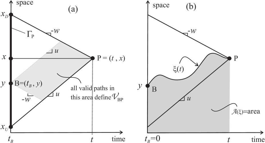
where $P$ is a generic point with coordinates $(t,x)$, $B\equiv(t_{B},y)$ is a point in the boundary $\Gamma^{P}$, $\xi$ is a member of the set of all valid paths between $B$ and $P$ denoted $\mathcal{V}_{BP}$, and $\xi(t_{B})=y$; see Fig. 1a. The function $R(\cdot)$ gives the maximum passing rates along the observer and corresponds to the (concave) Legendre transform of $\tilde{H}$, i.e.,

$$R(t,x,v)=\sup_{k}\left\{\tilde{H}(t,x,k)-vk\right\}.$$

It is worth mentioning that in the simplest homogeneous case where $\tilde{H}=H(k)$ the VT solution (8) becomes the Hopf-Lax formula:

$$N(P)=\min_{B\in\Gamma^{P}}\left\{G(B)+(t-t_{B})R\left(\frac{x-y}{t-t_{B}}\right)\right\},$$ (9)

where the minimization over $\xi(t)$ is no longer necessary since characteristics become straight lines in this case. Unfortunately, even the presence of exogenous lateral inflows that vary in time or space make characteristics not to be straight lines and therefore a Hopf-Lax type solution cannot be devised. A VT solution, however, still exists as shown next.

We now formulate VT solution to account for source terms explicitly. In the remaining of the paper, we assume a triangular flow-density diagram. It may be defined by its free-flow speed $u$, wave speed $-w$ (with $w>0$) and jam density $\kappa$ such that

$$H(k)=\min\left\{uk\ ,\ w(\kappa-k)\right\}\quad\mbox{for any}\quad k\in[0,\kappa].$$ (10)

It follows that the capacity is $Q=\kappa wu/(w+u)$ and the critical density $K=Q/u$.

When the potential function is exogenous, i.e. $\Phi=\Phi(t,x)$, the Hamiltonian can be written as the sum of the fundamental diagram and the potential function, i.e.: $\tilde{H}(t,x,k)=H(k)+\Phi(t,x)$. In the case of a triangular fundamental diagram we have $R(t,x,v)=Q-Kv+\Phi(t,x)$ with $v\in[-w,u]$, and the function $f(B,\xi)$ to be minimized reads:

$$f(B,\xi)=G(B)+(t-t_{B})Q-(x-y)K+\underbrace{\int_{t_{B}}^{t}\Phi(s,\xi(s))\ ds}_{J}$$ (11)

The $J$-integral in (11) is what separates this problem from the problems studied so far in traffic flow using VT principles. This integral in terms of $\phi$ is:

$$J=-\int_{t_{B}}^{t}\int_{y}^{\xi(s)}\phi(s,x)\ dxds,$$ (12)

and represents the net number of vehicles leaving the area below the curve $x=\xi(t)$, namely area $A(\xi)$; see Fig. 1b. Therefore, minimizing $J$ given $y=\xi(t_{B})$, can be interpreted as finding $\xi(t)$ that maximizes the net number of vehicles entering $A(\xi)$.

3.2 Initial value problems

In the initial value problem (IVP) the boundary $\Gamma$ is the line $\left\{t_{B}=0\right\}{\times\mathbb{R}}$, so that the problem here is (3a) supplemented with:

$$N(0,x)=G(x),$$ (13)

where we assume that $G\in C^{2}(\mathbb{R})$. The candidate set for $B,\Gamma^{P}$ is reduced to $B$’s $x$-coordinate, $y$, which is delimited by two points $U=(0,x_{U})$ and $D=(0,x_{D})$, where:

$$x_{U} =x-ut,\hskip 5.69054pt\mbox{and}\hskip 5.69054ptx_{D}=x+wt,$$ (14a)

$$x_{U} <y<x_{D}$$ (14b)

see Fig. 1a. The following subsections examine simplified versions of this problem that reveal considerable insight into the general solution.

3.2.1 Constant inflow

Consider the IVP with constant inflow problem:

$$\phi(t,x)=a,$$ (15)

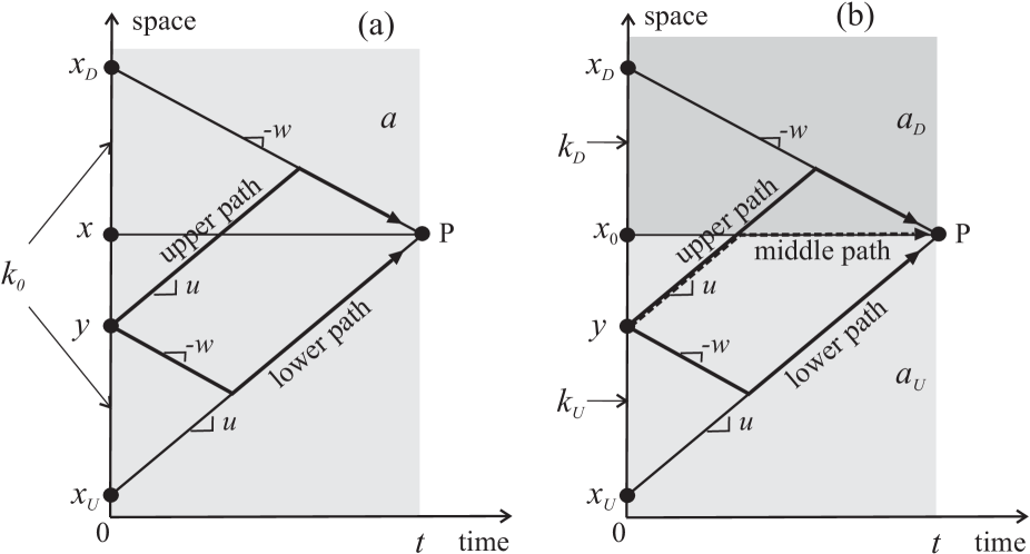
for some $a\in\mathbb{R}\setminus\{0\}$. It follows from (12) that $J=-aA(\xi)$ and therefore, for a fixed $y=\xi(0)$ the minimum of (11) is obtained by a path that: (i) maximizes $A(\xi)$ when $a>0$; or (ii) minimizes $A(\xi)$ when $a<0$. These two optimum paths are the extreme paths in $\mathcal{V}_{BP}$ that define its boundary; see “upper” and “lower” paths in Fig. 2a. This solution is a “bang-bang” solution, typical for this type optimal control problems. The reader can verify that the areas under these paths are given by $A(y,x_{D})$ and $A(y,x_{U})$, respectively, where we have defined:

$$A(y,x_{-})=\frac{1}{2}\left((x+x_{-})t-\text{sign}(a)\frac{\left(x_{-}-y\right){}^{2}}{u+w}\right)$$ (16)

where $\text{sign}(a)$ is the sign of $a$ and $x_{-}$ is a placeholder for $x_{D}$ if $a>0$ or $x_{U}$ if $a<0$. Thus the optimization problem has been reduced to a single variable, $y$, whose first- and second-order conditions for a minimum $y^{*}$ read:

$$f^{\prime}(y^{*}) =\psi\left(y^{*}-x_{-}\right)+G^{\prime}(y^{*})+K=0,$$ (17a)

$$f^{\prime\prime}(y^{*}) =\psi+G^{\prime\prime}(y^{*})>0,\hskip 14.22636pt\mbox{where:}$$ (17b)

$$\psi :=\frac{|a|}{u+w},$$ (17c)

where $|\cdot|$ denotes the absolute value. Notice that $\psi>0$ as long as $a\neq 0$.

Of course, the optimal point $y^{*}$ needs to satisfy (14b): $x_{U}\leq y^{*}\leq x_{D}$.

3.2.2 Constant initial density

Here, in addition to $\phi(t,x)=a,$ we assume

$$g(x)=k_{0},\hskip 28.45274pt-\infty<x<\infty$$ (18)

which implies that the function to minimize is a parabola:

$$f(y)=-c_{0}-c_{1}y+\frac{\psi}{2}y^{2},$$ (19)

with constants $c_{0}=Kx_{U}-\dfrac{\psi}{2}\left[x_{-}^{2}{-\text{sign}(a)}\left(x_{-}+x\right)(u+w)t\right]$ and $c_{1}=\psi x_{-}-(K-k_{0})$, and extremum:

$$y^{*}=x_{-}-\dfrac{K-k_{0}}{\psi}.$$ (20)

Notice that (17b) is always satisfied in this case and therefore $y^{*}$ is always a minimum and should be included so long as $x_{U}\leq y^{*}\leq x_{D}$. Combining this with (20) gives that the final solution can be expressed as:

$$f(y^{*}), t>(K-k_{0})/a>0$$ (21a)

$$\min\{f(x_{U}),f(x_{D})\},$$ otherwise (21b)

Notice that $(K-k_{0})/a$ represents the time it takes for the system to reach critical density, namely “time-to-capacity”. This means that $y^{*}$ will be the optimal candidate only once a regime transition occurs. This will happen only if the time to capacity is positive, i.e. when sign($a$) = sign($K-k_{0})$ or more explicitly, when $k_{0}$ is under-critical and $\phi$ is an inflow ($a$ positive) or when $k_{0}$ is over-critical and $\phi$ is an outflow ($a$ negative).

Somewhat unexpectedly, we note that $-f_{x}(x_{U})=-f_{x}(x_{D})=-f_{x}(y^{*})=k_{0}+at$, which means that the density is always given by the traveling wave $k(t,x)=k_{0}+at$, which is also the solution of (1) in this case using the method of characteristics. One should also impose feasibility conditions for the density, i.e. $0\leq k\leq\kappa$, which gives:

$$0, t>-k_{0}/a,a<0$$ (22a)

$$\kappa, t>(\kappa-k_{0})/a,a>0$$ (22b)

$$k_{0}+at,$$ otherwise (22c)

The flow can be obtained using (5), but it is equivalent and simpler to use $q=H(k)$.

3.2.3 Extended Riemann problems

Riemann problems are the building blocks of Godunov-type numerical solution methods. As illustrated in Fig. 2b, in these problems one is interested in the value of $N$ at $x=x_{0}\geq ut$, i.e. at point $P=(t,x_{0})$, with initial data typically given by the density at $t=0$. This is a very special case for with the ‘target’ point $P$ is located on the discontinuity of the initial data at $x=x_{0}$. However the methodology below can be easily extended to the cases where $P=(t,x)$ with $x<x_{0}$ or $x>x_{0}$. Here, we extend the initial data to include the inflow:

$$(k_{U},a_{U}),\hskip 28.45274ptx\leq x_{0}$$ (23a)

$$(k_{D},a_{D}),\hskip 28.45274ptx>x_{0},$$ (23b)

which in conjunction with (3) define an extended Riemann problem, or ERP for short. We assume that $\left(a_{U},a_{D}\right)\neq(0,0)$. Notice that now:

$$x_{U}=x_{0}-ut,\hskip 5.69054pt\mbox{and}\hskip 5.69054ptx_{D}=x_{0}+wt.$$ (24)

For simplicity and without loss of generality we set $G(x_{0})=0$, which implies:

$$(x_{0}-x)k_{U},\hskip 28.45274ptx\leq x_{0}$$ (25a)

$$(x_{0}-x)k_{D},\hskip 28.45274ptx>x_{0}$$ (25b)

It will be convenient to define:

$$\eta=a_{U}/a_{D},\hskip 28.45274pt\psi=\frac{a_{D}}{u+w},\hskip 28.45274pt\theta=u/w.$$ (26)

The $J$-integral in this case is a weighted average of the portion of $A(\xi)$ upstream and downstream of $x=x_{0}$, weighted by $a_{U}$ and $a_{D}$, respectively. For instance, if $\xi(t)>0$ for all $t$, we have $J=-\int_{0}^{t}\int_{0}^{\xi(t)}\phi(x)\ dxdt=-\int_{0}^{t}(a_{U}x_{0}+a_{D}(\xi(t)-x_{0}))dt=-(a_{U}x_{0}t+a_{D}\int_{0}^{t}\xi(t)-x_{0}dt),$ where $x_{0}t$ is the portion of $A(\xi)$ upstream of $x=x_{0}$ and $\int_{0}^{t}\xi(t)-x_{0}dt$ is the portion of $A(\xi)$ downstream of $x=x_{0}$ in this particular case.

It follows that the minimization of the $J(\xi)$ can be achieved analogously to the previous section by considering the upper and lower paths from each candidate $y=\xi(0)$. In addition, however, one has to include 2 middle “paths” that would reach and stay at $x=x_{0}$ until reaching $P$; see Fig. 2b. To formalize, let $j_{1},j_{2}$ and $j_{3}$ be the value of $J(\xi)$ when $y\geq x_{0}$ along the upper, lower and middle paths, respectively; similarly for $j_{4},j_{5}$ and $j_{6}$ when $y\leq x_{0}$. Calculating the areas upstream and downstream of $x=x_{0}$ defined by each path, it can be shown that the $j_{i}$’s can be obtained from:

$$2(j_{1}(y)-J_{0})/\psi =-\theta t^{2}w^{2}(2\eta(\theta+1)+1)+2twy_{0}+y_{0}^{2},$$ (27a)

$$2(j_{2}(y)-J_{0})/\psi =-\eta\theta(2\theta+1)t^{2}w^{2}+2\eta\theta twy_{0}+y_{0}^{2}((\eta-1)\theta-1),$$ (27b)

$$2(j_{3}(y)-J_{0})/\psi =-(\theta+1)\left(2\eta\theta t^{2}w^{2}+y_{0}^{2}\right),$$ (27c)

$$2(j_{4}(y)-J_{0})/\psi =-\theta t^{2}w^{2}(2\eta(\theta+1)+1)+2twy_{0}+y_{0}^{2}(\eta\theta+\eta-1)/\theta,$$ (27d)

$$2(j_{5}(y)-J_{0})/\psi =-\eta\left(\theta(2\theta+1)t^{2}w^{2}-2\theta twy_{0}+y_{0}^{2}\right),$$ (27e)

$$2(j_{6}(y)-J_{0})/\psi =\eta(\theta+1)\left(y_{0}^{2}-2\theta^{2}t^{2}w^{2}\right)/\theta,$$ (27f)

where $y_{0}=x_{0}-y$ and $J_{0}$ is a constant of our problem that represents the net number of vehicles leaving the area upstream of $x_{U}$, i.e. $-a_{U}x_{U}t$ in this case. Notice that $j_{1}(x_{0})=j_{4}(x_{0}),j_{2}(x_{0})=j_{5}(x_{0})$ and $j_{3}(x_{0})=j_{6}(x_{0})$, as expected. The function to minimize in this case can be written as:

$$f(y)=G(y)+tQ-(x_{0}-y)K+J(y),\hskip 14.22636pt\mbox{where:}$$ (28)

$$\min\{j_{1}(y),j_{2}(y),j_{3}(y)\}, y>x_{0}$$ (29a)

$$\min\{j_{4}(y),j_{5}(y),j_{6}(y)\}, y\leq x_{0}$$ (29b)

The solution of (3) under these conditions can be reduced to the evaluation of $f(y)$ at a small number of candidates. In addition to candidates $y=x_{U}$ and $y=x_{D}$, we have to consider the discontinuity at $y=x_{0}$ and the possible minima produced by each of the components in (27). Since $f(y)$ is piecewise quadratic, each one of these components has at most one minimum, namely $y=y_{i},i=1,\ldots 6$, which can be obtained by solving the first-order conditions $f(y_{i})=0$ associated with each of the $j_{i}$’s; i.e.:

$$y_{1} =x_{D}-(K-k_{D})/\psi,\hskip 28.45274pty_{2}=x_{0}+\frac{\eta\theta x_{D}-(K-k_{D})/\psi}{\theta(\eta-1)-1},$$ (30a)

$$y_{3} =x_{0}+\frac{K-k_{D}}{(\theta+1)\psi},\hskip 45.52458pty_{4}=x_{0}+\frac{x_{U}+\theta(K-k_{U})/\psi}{1-\eta(1+\theta)},$$ (30b)

$$y_{5} =x_{U}+(K-k_{U})/(\eta\psi),\hskip 14.22636pty_{6}=x_{0}+\frac{\theta\left(k_{U}-K\right)}{\eta(\theta+1)\psi},$$ (30c)

For the $y_{i}$’s to be valid candidates they must meet the following conditions:

$$x_{0}<y_{i}<x_{D},\hskip 56.9055pt i=1,2,3$$ (31a)

$$x_{U}<y_{i}<x_{0},\hskip 56.9055pt i=4,5,6$$ (31b)

which ensure that $y_{i}$ is on the boundary $\Gamma^{P}$. With all, the sought solution can be expressed as:

$$N(t,x_{0})=\min_{y\in\mathcal{Y}}f(y),\hskip 14.22636pt\mbox{with: }\mathcal{Y}=\{x_{U},x_{0},x_{D},y_{1}^{*},\ldots y_{6}^{*}\}$$ (32)

where $y_{i}^{*}$ is $y_{i}$ if (31) is met and null otherwise. Notice that this solution method does not require imposing $f^{\prime\prime}(y^{*})>0$ because maxima will be automatically discarded in the minimum operation.

The average flow $\bar{q}(t,x_{0})$ during $(0,t)$ can be obtained as follows:

$$\bar{q}(t,x_{0}) =\frac{1}{t}\int_{0}^{t}N_{t}(s,x_{0})-\Phi(s,x_{0})\ ds=\frac{1}{t}(N(t,x_{0})-\int_{0}^{t}\Phi(s,x_{0})\ ds)$$ (33a)

$$=\frac{1}{t}(N(t,x_{0})-(J_{0}+x_{U}a_{U})t)=N(t,x_{0})/t-J_{0}-x_{U}a_{U}.$$ (33b)

As shown in Section 4, this formula allows to formulate improved numerical solution methods for the endogenous problem.

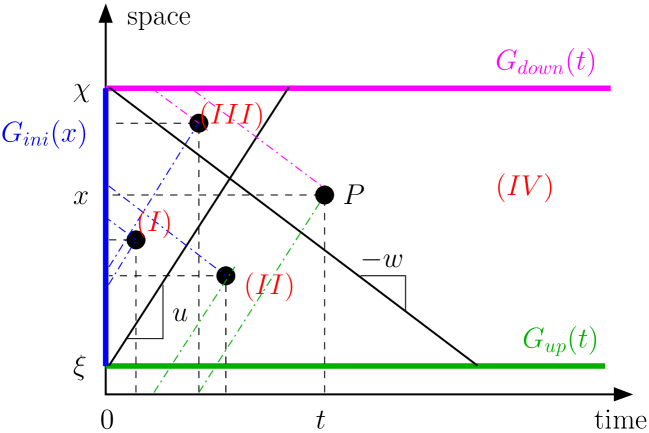
3.3 Initial and boundary value problem

We restrict the space to a segment of road $[\xi,\chi]$ with $\xi<\chi$. In the initial and boundary value problem (IBVP) the boundary $\Gamma$ is the set defined as

$$\left(\left\{t_{B}=0\right\}\times[\xi,\chi]\right)\cup\left((0,+\infty)\times\left\{x=\xi\right\}\right)\cup\left((0,+\infty)\times\left\{x=\chi\right\}\right),$$

so that the problem here is (3a) supplemented with:

$$\begin{cases}N(0,x)=G_{ini}(x),\quad&\mbox{on}\quad[\xi,\chi],\\ N(t,\xi)=G_{up}(t),\quad&\mbox{on}\quad(0,+\infty),\\ N(t,\chi)=G_{down}(t),\quad&\mbox{on}\quad(0,+\infty).\end{cases}$$ (34)

For obvious compatibility reasons, we request these conditions to satisfy

$$G_{ini}(\xi)=G_{up}(0)\quad\mbox{and}\quad G_{ini}(\chi)=G_{down}(0).$$

We also consider a $a\neq 0$ and $k_{0}\in[0,\kappa]$ such that the inflow rate is given by

$$\varphi(t,x)=a,\quad\mbox{for any}\quad(t,x)\in[0,+\infty)\times[\xi,\chi]$$

and the initial density

$$g_{ini}(x)=k_{0},\quad\mbox{for any}\quad x\in[\xi,\chi].$$

According to the position of point $P=(t,x)$ with $t>0$ and $x\in(\xi,\chi)$, we have the following cases to distinguish (in the spirit of Jin (2015))

$$\left(t_{U},x_{U}\right)=\begin{cases}\left(0,x-\dfrac{t}{u}\right),\quad&\mbox{if}\quad x\geq\xi+\dfrac{t}{u},\\ \left(t-\dfrac{x-\xi}{u},\xi\right),\quad&\mbox{else},\end{cases}$$

and

$$\left(t_{D},x_{D}\right)=\begin{cases}\left(0,x+\dfrac{t}{w}\right),\quad&\mbox{if}\quad x\leq\chi-\dfrac{t}{w},\\ \left(t+\dfrac{x+\chi}{w},\chi\right),\quad&\mbox{else},\end{cases}$$

that define 4 regions (see Figure 6)

$$\begin{array}[]{rccc}\text{Region}&\text{Set of points}&\text{Upstream point}&\text{Downstream point}\\ I:&\left\{(t,x)\ \left|\ \chi-\dfrac{t}{w}\geq x\geq\xi+\dfrac{t}{u}\right.\right\}&\left(t_{U},x_{U}\right)=\left(0,x-\dfrac{t}{u}\right)&\left(t_{D},x_{D}\right)=\left(0,x+\dfrac{t}{w}\right)\\ \\ II:&\left\{(t,x)\ \left|\ x\leq\min\left\{\xi+\dfrac{t}{u},\chi-\dfrac{t}{w}\right\}\right.\right\}&\left(t_{U},x_{U}\right)=\left(t-\dfrac{x-\xi}{u},\xi\right)&\left(t_{D},x_{D}\right)=\left(0,x+\dfrac{t}{w}\right)\\ \\ III:&\left\{(t,x)\ \left|\ x\geq\max\left\{\xi+\dfrac{t}{u},\chi-\dfrac{t}{w}\right\}\right.\right\}&\left(t_{U},x_{U}\right)=\left(0,x-\dfrac{t}{u}\right)&\left(t_{D},x_{D}\right)=\left(t+\dfrac{x+\chi}{w},\chi\right)\\ \\ IV:&\left\{(t,x)\ \left|\ \xi+\dfrac{t}{u}\geq x\geq\chi-\dfrac{t}{w}\right.\right\}&\left(t_{U},x_{U}\right)=\left(t-\dfrac{x-\xi}{u},\xi\right)&\left(t_{D},x_{D}\right)=\left(t+\dfrac{x+\chi}{w},\chi\right)\end{array}$$

To be continued but the idea is that in Region I, everything is exactly the same than in previous Subsection 3.2 while in the other cases, we will compare initial data $G_{ini}$ coming from $(t_{D},x_{D})$ with upstream data $G_{up}$ coming from $(t_{U},x_{U})$ (Region II), initial data $G_{ini}$ from $(t_{U},x_{U})$ with downstream data $G_{down}$ from $(t_{D},x_{D})$ (Region III) and finally upstream data $G_{up}$ from $(t_{U},x_{U})$ and downstream data $G_{down}$ from $(t_{D},x_{D})$ (Region IV). I feel that everything can be done exactly in the same way and finally the idea is to use the inf-morphism from Aubin, Bayen, Saint-Pierre (2006)

$$N(t,x)=\min\left\{N_{ini}(t,x)\ ,\ N_{up}(t,x)\ ,\ N_{down}(t,x)\right\}.$$

4 Numerical solution methods

In the following two subsections we formulate two numerical solution methods to find the global solution of the endogenous inflow problem in conservation law form (1), (7) and in HJ form (3), (7), respectively. The basic idea is that in discrete time, if the (endogenous) inflows are computed using the traffic states from the previous time step using an explicit-in-time numerical scheme, then they become exogenous for the current time step and therefore the VT solution may be applied.

4.1 Godunov’s method

This method has been traditionally used to solve the traffic problem in conservation law form without inflows, and constitutes the basis of the well known Cell Transmission (CT) model (Daganzo, 1994) assuming the triangular Hamiltonian (10). In this method, time and space are discretized in increments $\Delta t$ and $\Delta x=u\Delta t$, respectively, and we let:

$$k_{i}^{j}=k(j\Delta t,i\Delta x)$$ (35)

be the numerical approximation of the density. The update scheme is the following discrete approximation of the conservation law (1):

$$\frac{k_{i+1}^{j}-k_{i}^{j}}{\Delta t}+\frac{q_{i}^{j+1}-q_{i}^{j}}{\Delta x}=\phi(k_{i}^{j})$$ (36)

The key to Godunov’s method is the computation of the flow into cell $i,q_{i}^{j}$, which are obtained by solving Riemann problems. Traditionally, inflows have been considered explicitly only in the update scheme (36) but not in the solution of the Riemann problems (Laval and Leclercq, 2010). This implies that the computation of $q_{i}^{j}$ corresponds to the original CT rule:

$$q_{i}^{j}=\min\{Q,uk_{i}^{j},(\kappa-k_{i}^{j+1})w\},\hskip 85.35826pt\mbox{(CT rule)}$$ (37)

Here, we will compare the CT rule with the ERP rule (33b), i.e. the flow based on extended Riemann problems. Both methods are first-order accurate since both are Godunov-type methods, and therefore the rate of convergence of both methods should be similar and roughly proportional to the mesh size. The main difference is in the magnitude of the error, where the ERP rule should be more accurate because the impacts of inflows are explicitly considered in the solution of Riemann problems. We illustrate this with the following example.

Example. Consider an empty freeway at $t=0$ subject to an inflow linear in both $x$ and $k$; i.e.:

$$g(x) =0,$$ (38a)

$$\phi(k) =ax-buk,\hskip 28.45274pta,b>0.$$ (38b)

Notice that (Laval and Leclercq, 2010) showed that linear inflow functions arise in the continuum approximation of the Newell-Daganzo merge model (Newell, 1982; Daganzo, 1994), which accounts for the interactions between freeway and on-ramp demands. The particular coefficients of the linear function depend upon the state of the freeway and on-ramps. In particular, (38b) corresponds to the case where both are in free-flow, $ax$ represent the inflow demand rate at $x$ and $b$ the exit probability per unit distance. Using the method of characteristics (Laval and Leclercq, 2010) showed that the solution of (1), (38) is :

$$k(t,x)=\frac{a}{b^{2}u}\left(bx-1+(1-b(x-tu))e^{-btu}\right)$$ (39)

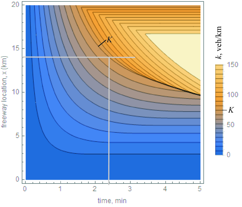
provided $k(t,x)\leq K$. To get an idea of the solution for all densities, Fig. 3 shows the numerical ERP solution with $\Delta t=1$ s, with parameters given in its caption. Notice that similarly to Laval and Leclercq (2010) we chose $\theta=1$ to avoid the numerical errors intrinsic to Godunov’s method and to focus on those caused by the treatment of the inflow.

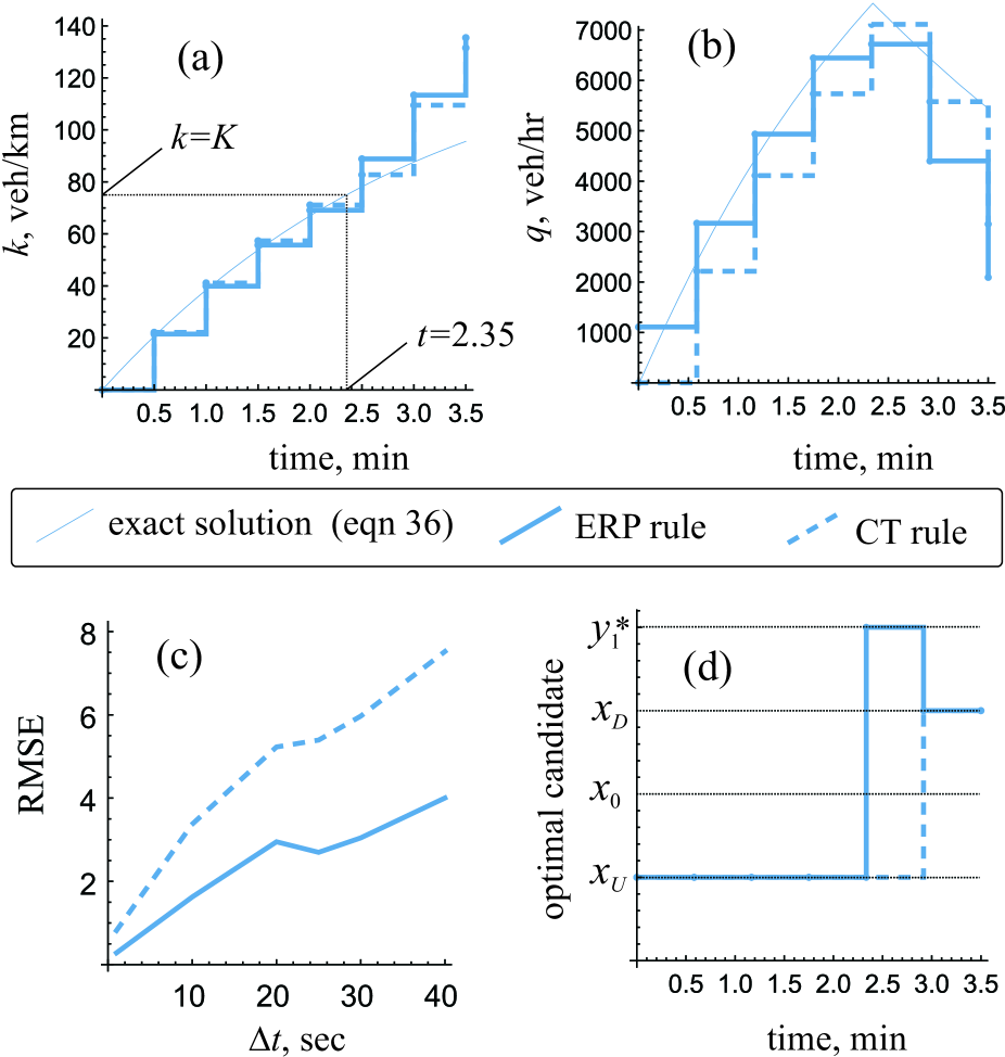
Fig. 4 compares the CT-rule with the ERP-rule numerical solution (with $\Delta t=40$ s) for this example vis-a-vis the exact solution (39). Parts (a) and (b) show the time evolution of the density and flow, respectively, at $x=14$ km obtained with each method. It can be seen that the main difference, as expected, is in the flow estimates, particularly at $t=0$ where the CT rule predicts zero flow since the freeway is empty and it does not consider inflows in its calculations.

To assess the accuracy of each method, part (c) of Fig. 4 shows the density root-mean-squared error (RMSE) of each method with respect to (39) for varying $\Delta t$ and only until $t=2.35$ s, when the density exceeds the critical density $K$; see Fig. 4a. It becomes apparent that both methods converge to the right solution as $\Delta t\rightarrow 0$, but the accuracy of the proposed method outperforms the existing method by a factor of two for all values of $\Delta t$.

Fig. 4d shows the optimal candidate that minimizes $f(y)$ at each time step of the numerical method, which is an element of the set $\mathcal{Y}$, for the ERP rule, and of $\{x_{U},x_{0},x_{D}\}$ for the CT rule. It can be seen that both methods coincide except for the time step where the density approaches the critical density, in which case the proposed method finds the more accurate optimal candidate $y_{1}^{*}$.

4.2 Variational networks

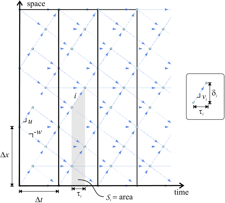
Daganzo (2005b) introduced time-space networks to solve the traffic problem without inflows in variational form using shortest paths. Notice that this is an application of Bellman’s dynamic programming principle. Each link $i$ in these “variational networks” is defined by its: (i) slope $v_{i}$: wave speed, (ii) cost $c_{i}$: maximum number of vehicles that can pass, (iii) time length $\tau_{i}$, and (iv) distance length $\delta_{i}=\tau_{i}v_{i}$; see inset in Fig. 5.

Since the fundamental diagram is assumed triangular and the freeway homogeneous, there are only three wave speeds to be considered, $u,-w$ and $0$, and the corresponding passing rates are given by

$$w\kappa, v_{i} =-w$$ (40a)

$$Q, v_{i} =0$$ (40b)

$$0, v_{i} =u$$ (40c)

Let $J_{i}$ be the contribution of the $J$-integral in the cost of each link $i$. It corresponds to the (negative of) integral of $\phi(t,x)$ over the shaded region in Fig. 5, $\mathcal{S}_{i}$, and can be approximated by:

$$J_{i} =-\tau_{i}\sum_{j\in\mathcal{S}_{i}}\delta_{j}a_{j},$$ (41a)

where $a_{j}$ is the inflow associated with link $j$ and $j\in\mathcal{S}_{i}$ means all links that “touch” area $\mathcal{S}_{i}$. Finally, the cost to be used in each link becomes:

$$c_{i}=\mathcal{L}(v_{i})\tau_{i}+J_{i}.$$ (42)

The advantage of this method is that it is free of numerical errors (when inflows are exogenous) but it may be cumbersome to implement unless $\theta$ is an integer. In that case, as illustrated in Fig. 5 for $\theta=2$, the location of nodes align on a grid pattern. This allows defining a conventional grid with cell size $\Delta t,\Delta x$ where inflows may be assumed constant. The other disadvantage is that merge models are typically expressed in terms of flows or densities rather than $N$ values, and therefore an additional computational layer has to be added.

5 Other coordinates

As pointed out in Laval and Leclercq (2013) there are two additional coordinate systems that provide alternative solution methods of the traffic flow problems without inflows. In space-Lagrangian coordinates the quantity of interest is $X(t,n)$, the position of vehicle $n$ at time $t$; in time-Lagrangian coordinates one is interested in $T(n,x)$, the time vehicle $n$ crosses location $x$.

These representations correspond to the same surface in the three-dimensional space of vehicle number, time and distance, but expressed with respect to a different coordinate system. We briefly analyze these two alternatives when considering Eulerian source terms and conclude that even if a HJ equation is still valid in both cases, one cannot expect to get a VT representation formula even when inflows $\phi(t,x)$ are exogenous.

5.1 Space-Lagrangian coordinates: X-models

Let $s(t,n)$ be the spacing of vehicle $n$ at time $t$. To derive the X-model we multiply the N-model (3a) by $s$ to get $sN_{t}-sH(k)=s\Phi(t,x)$. Noting that $s=-X_{n}$ and $sN_{t}=-X_{n}N_{t}=X_{t}$, this can be rewritten as:

$$X_{t}-V(-X_{n})=-X_{n}\Phi(t,X),$$ (43)

where $V(s)=sH(1/s)$ is this spacing-speed fundamental diagram. We conclude that (43) is still a HJ PDE but does not admit a VT solution due to the term involving $X$. The corresponding conservation law can be obtained by taking the partial derivative with respect to $n$ of (43):

$$s_{t}+V(s)_{n}=-\phi(t,X)s^{2}-\Phi(t,X)s_{n},$$ (44)

Notice that van Wageningen-Kessels et al. (2013) identified (44) but without the term $\Phi(t,X)s_{n}$ using a different approach, and used it to formulate a numerical solution method in the case of discrete inflows.

5.2 Time-Lagrangian coordinates: T-models

Let $r=T_{x}$ and $h=1/q$ be the pace and the headway of vehicle $n$ at location $x$, and let $F(r)$ be the fundamental diagram in this case, i.e. $h=F(r)$. Here, the T-model is simply $F(r)=1/q$, where $q$ is given by $q=N_{t}-\Phi(t,x)$, per (5). Noting that $N_{t}=1/T_{n}$ this can be rewritten as:

$$T_{n}-\frac{F(T_{x})}{1+\Phi(T,x)F(T_{x})}=0,$$ (45)

which, again, is still a HJ PDE but does not admit a VT solution due to the term involving $T$. The corresponding conservation law can be obtained by taking the partial derivative with respect to $x$ of (45):

$$r_{n}-\frac{F(r)_{x}+F(r)^{2}\phi(T,x)}{(1+\Phi(T,x)F(r))^{2}}=0.$$ (46)

To summarize, it becomes apparent that in Lagrangian and vehicle number-space coordinates the solution to our problem does not accept VT solutions and therefore becomes more difficult to solve.

6 Discussion

We have shown in this paper that VT solutions to the traffic flow problem exist only in Eulerian coordinates when inflows are exogenous. In all other cases the Hamiltonian is a non-local function of the independent variable, and the corresponding variational may not be possible to formulate. Even in the simplest endogenous linear case (7) the reader can appreciate the mathematical difficulties: using $\Phi=\Phi(s,N(s,\xi(s)))$ in (8a)-(11) turns the problem implicit in $N$, and therefore it is no longer a VT problem.

Improved numerical solution methods for the endogenous case were derived by taking advantage of this insight. In other fields, it appears that solving the extended Riemann problems explicitly considering the inflows has not been possible, and the only alternative has been to use high-resolution Riemann solvers (Schroll and Winther, 1996; LeVeque, 1998). We have shown that this is not the case in traffic flow, and that the ERP method presented here is indeed more accurate.

A streamlined version of the ERP method could be envisioned that drastically improves computation times with minimal impact in the quality of the solution. To see this, recall that Fig. 4d showed that the candidate $y_{1}^{*}$ was optimal only during the time step where the density approaches the critical density. Based on the discussion following eqn. (40) it is reasonable to conjecture that candidates $y_{1}^{*},y_{2}^{*}\ldots y_{6}^{*}$ in (32) would be optimal only when a transition takes place. Therefore, the streamlined method would consider only the reduced set $\mathcal{Y}=\{x_{U},x_{0},x_{D}\}$ in (32), which would induce an error only in the time step where the transition occurs. This error can be made arbitrarily small by decreasing $\Delta t$. Notice that this does not mean that the continuum solution (32) can be streamlined in this way; this is only possible in discrete time where $N$-values are updated at each time step.

The implications of our findings in the context of MFD analytical approximation methods considering turns as a continuum inflow are not encouraging. This is because inflows in this case would have to be endogenous for the method to be meaningful, and in such case we have seen that there is no VT solution. This implies that the method of cuts–the only method used so far to provide analytical MFD approximations–is no longer applicable. At the same time, however, a stochastic extension of the method of cuts proved successful in approximating a real-life MFD (Laval and Castrillon, 2015). This would indicate that, at least in the context of the MFD, VT solutions still provide good approximations. Research in this topic is ongoing.

References

Figure 1: Illustration of key definitions in VT: (a) the initial value problem; (b) the area of the integration to obtain the $J$-integral.

Figure 2: Possible paths to minimize the $J$-integral: (a) constant initial density; (b) extended Riemann problems.

Figure 3: Numerical ERP solution of (38) with $\Delta t=1$ s and parameters: freeway length $L$ = 20 km, $w$ = 100 km/hr, $\kappa$ = 150 veh/km, $\theta$ = 1, $a=0.5Q/L$, $b=0.3$.

Figure 4: Comparison of the CT rule with the ERP rule solution for the example in §4. (a) and (b): density and flow at $x=14$ km, (c) candidate number that minimizes $f(y)$, (d) RMSE of each method for varying $\Delta t$.

Figure 5: Variational networks: time-space networks to solve the traffic problem with inflows using shortest paths.

Figure 6: The four different regions to consider for an Initial and Boundary Value Problem with initial data $G_{ini}$, upstream $G_{up}$ and downstream $G_{down}$ boundary conditions.

References

- Barron et al. (1996) Barron, E., Jensen, R., Liu, W., 1996. Hopf-Lax-type formula for . Journal of Differential Equations 126 (1), 48 – 61.
- Barron (2015) Barron, E. N., 2015. Representation of viscosity solutions of hamilton-jacobi equations. Minimax Theory and its Applications 1 (1).
- Costeseque and Lebacque (2014a) Costeseque, G., Lebacque, J.-P., 2014a. Discussion about traffic junction modelling: Conservation laws vs Hamilton-Jacobi equations. Discrete and Continuous Dynamical Systems - Series S 7 (3), 411–433.
- Costeseque and Lebacque (2014b) Costeseque, G., Lebacque, J.-P., 2014b. A variational formulation for higher order macroscopic traffic flow models: numerical investigation. Transportation Research Part B: Methodological 70, 112–133.
- Daganzo (1994) Daganzo, C. F., 1994. The cell transmission model: A dynamic representation of highway traffic consistent with the hydrodynamic theory. Transportation Research Part B 28 (4), 269–287.
- Daganzo (2005a) Daganzo, C. F., 2005a. A variational formulation of kinematic wave theory: basic theory and complex boundary conditions. Transportation Research Part B 39 (2), 187–196.
- Daganzo (2005b) Daganzo, C. F., 2005b. A variational formulation of kinematic waves: Solution methods. Transportation Research Part B: Methodological 39 (10), 934 – 950.
- Daganzo (2014) Daganzo, C. F., 2014. Singularities in kinematic wave theory: Solution properties, extended methods and duality revisited. Transportation Research Part B: Methodological 69, 50 – 59.
- Daganzo and Geroliminis (2008) Daganzo, C. F., Geroliminis, N., 2008. An analytical approximation for the macroscopic fundamental diagram of urban traffic. Transportation Research Part B: Methodological 42, 771–781.
- Evans (1998) Evans, L. C., Jun. 1998. Partial Differential Equations (Graduate Studies in Mathematics, V. 19) GSM/19. American Mathematical Society.
- Geroliminis and Boyacı (2013) Geroliminis, N., Boyacı, B., 2013. The effect of variability of urban systems characteristics in the network capacity. Transportation Research Part B 46(10), 1576–1590.
- Hopf (1970) Hopf, E., 1970. On the right weak solution of the cauchy problem for a quasilinear equation of first order. Indiana Univ. Math. J. 19, 483–487.
- Jin (2015) Jin, W.-L., 2015. Continuous formulations and analytical properties of the link transmission model. Transportation Research Part B: Methodological 74, 88–103.
- Laval and Castrillon (2015) Laval, J., Castrillon, F., 2015. Stochastic approximations for the macroscopic fundamental diagram of urban networks. Transportation Research Part B (In press, also in 21th International Symposium of Transportation and Traffic Theory).
- Laval and Leclercq (2010) Laval, J. A., Leclercq, L., 2010. Continuum approximation for congestion dynamics along freeway corridors. Transportation Science (44), 87–97.
- Laval and Leclercq (2013) Laval, J. A., Leclercq, L., 2013. The Hamilton-Jacobi partial differential equation and the three representations of traffic flow. Transportation Research Part B 52, 17–30.
- Lax (1957) Lax, P. D., 1957. Hyperbolic systems of conservation laws ii. In: Sarnak, P., Majda, A. (Eds.), Communications on Pure and Applied Mathematics. Wiley Periodicals, p. 537 1 7566.
- Leclercq and Geroliminis (2013) Leclercq, L., Geroliminis, N., 2013. Estimating MFDs in simple networks with route choice. Transportation Research Part B: Methodological 57, 468–484.
- Leclercq et al. (2007) Leclercq, L., Laval, J. A., Chevallier, E., 2007. The Lagrangian coordinates and what it means for first order traffic flow models. In: Transportation and Traffic Theory 2007. Papers Selected for Presentation at ISTTT17.
- LeVeque (1998) LeVeque, R. J., 1998. Balancing source terms and flux gradients in high-resolution Godunov methods: The quasi-steady wave-propagation algorithm. J. Comput. Phys. 146, 346–365.
- LeVeque (1993) LeVeque, R. L., 1993. Numerical methods for conservation laws. Birkhauser Verlag.
- Lighthill and Whitham (1955) Lighthill, M. J., Whitham, G., 1955. On kinematic waves. I Flow movement in long rivers. II A theory of traffic flow on long crowded roads. Proceedings of the Royal Society of London 229 (A), 281–345.
- Newell (1982) Newell, G. F., 1982. Applications of queueing theory, 2nd Edition. Chapman Hall, London, U.K.
- Newell (1993) Newell, G. F., 1993. A simplified theory of kinematic waves in highway traffic, I general theory, II queuing at freeway bottlenecks, III multi-destination flows. Transportation Research Part B 27 (4), 281–313.
- Olejnik (1957) Olejnik, O., 1957. Discontinuous solutions of non-linear differential equations. Translated by George Biriuk. Am. Math. Soc., Transl., II. Ser. 26, 95–172.
- Richards (1956) Richards, P. I., 1956. Shockwaves on the highway. Operations Research (4), 42–51.
- Schroll and Winther (1996) Schroll, H. J., Winther, R., 1996. Finite difference schemes for scalar conservation laws with source terms. IMA J. Numer Anal 16, 201–215.
- van Wageningen-Kessels et al. (2013) van Wageningen-Kessels, F., Yuan, Y., Hoogendoorn, S. P., van Lint, H., Vuik, K., 2013. Discontinuities in the lagrangian formulation of the kinematic wave model. Transportation Research Part C: Emerging Technologies 34, 148 – 161.