A Nonlinear Adaptive Filter Based on the Model of Simple Multilinear Functionals

Abstract

Nonlinear adaptive filtering allows for modeling of some additional aspects of a general system and usually relies on highly complex algorithms, such as those based on the Volterra series. Through the use of the Kronecker product and some basic facts of tensor algebra, we propose a simple model of nonlinearity, one that can be interpreted as a product of the outputs of K FIR linear filters, and compute its cost function together with its gradient, which allows for some analysis of the optimization problem. We use these results it in a stochastic gradient framework, from which we derive an LMS-like algorithm and investigate the problems of multi-modality in the mean-square error surface and the choice of adequate initial conditions. Its computational complexity is calculated. The new algorithm is tested in a system identification setup and is compared with other polynomial algorithms from the literature, presenting favorable convergence and/or computational complexity.

I Introduction

The collective of nonlinear signal processing techniques come into play whenever nonlinear effects, such as harmonic distortion, saturation and general polynomial behavior, start to become noticeable enough to degrade the performance of conventional linear techniques. A common problem with nonlinear filters is the computational complexity they demand. Some of the most complex filters are based on the Volterra and Wiener models[1, 2, 3]. It is common to restrict these models in order to reduce their complexity [4, 5, 6]. We follow this approach.

We start by proposing a polynomial technique that could be thought of as a subclass of the Volterra model. It is based on representing the input regressor as an iterated Kronecker product, an idea that has already been used for the estimation of higher order statistics of the regressor [7]—a related problem—and other Volterra approaches [4, 5, 6], but we also embed this Kronecker structure within the filter itself. This formalism allows us to promptly derive a cost function in explicit form. We also compute its gradient and use it in the derivation of a nonlinear, low-complexity, LMS-like algorithm with good mean-square performance.

II Simple Multilinear Model

The general $K$-th order homogeneous Volterra kernel is a function $h(i_{1},\dotsc,i_{K})$ used to produce the input/output relationship in (1). There, $u(i)$ is the input signal and $M$ is the length of the filter.

$$y(i)=\sum_{0\leq i_{1},\dotsc,i_{K}<M}h(i_{1},\dotsc,i_{K})u(i-i_{1})\dotsb u(i-i_{K})$$ (1)

Evaluating (1) is a highly complex task. One would take $O(M^{K})$ operations per iteration. This can be slightly reduced should the symmetry in the kernel be explored, but this approach could at most decrease the number of operations to something proportional to $M-K+1\choose K$, which still increases rapidly. It is necessary to suppose some extra structure in the kernel itself if one wants a significant reduction in complexity.

The structure we propose is kernel separability. Explicitly, we suppose that there exists functions $h_{s}(i_{s})$, $1\leq s\leq K$, such that

$$h(i_{1},\dotsc,i_{K})=h_{1}(i_{1})h_{2}(i_{2})\dotsm h_{K}(i_{K}).$$ (2)

When we use (2) in (1), we get

$$y(i) =\sum_{0\leq i_{1},\dotsc,i_{K}<M}h_{1}(i_{1})\dotsm h_{K}(i_{K})u(i-i_{1})\dotsm u(i-i_{K})$$

$$=\sum_{i_{1}=0}^{M-1}h_{1}(i_{1})u(i-i_{1})\dotsb\sum_{i_{K}=0}^{M-1}h_{K}(i_{K})u(i-i_{K}).$$ (3)

Each factor $y_{os}(i)\triangleq\sum_{i_{s}=0}^{M}h_{s}(i_{j})u(i-i_{s})$ could be seen as the output of a linear FIR filter. As such, we can represent them in vector form. We collect the input signals in a $1\times M$ row vector $u_{i}=[u(i)\,u(i-1)\cdots u(i-M+1)]$ and a set of $K$ vectors of size $M\times 1$ represented by $\{w_{1},\dotsc,w_{K}\}$. We also say that, for each $s$, we have

$$w_{s}=[h_{s}(0)\,h_{s}(1)\cdots h_{s}(M-1)]^{T}.$$ (4)

Now, we have $y_{os}(i)=u_{i}w_{s}$ for every $s$, so that

$$y(i)=(u_{i}w_{1})(u_{i}w_{2})\dotsb(u_{i}w_{K}).$$ (5)

This can be represented by Fig. 1. Granted, this implies a loss of generality from the original Volterra model. Not every kernel is separable. But this simplification allows us to compute the output of the system in $O(KM)$ operations per iteration—a exponential reduction in complexity. Moreover, this separable kernel allows a convenient formalism for the derivation of the cost function that also gives us algebraic insight on the model.

Figure 1: Block diagram of the Simple Multilinear Model.

II-A Kronecker Representation

Using the identity $(A\otimes B)(C\otimes D)=(AC)\otimes(BD)$ for the Kronocker product [9], it follows that (5) is equivalent to (II-A), because the Kronecker product of scalars is their ordinary multiplication.

$$y(i) =(u_{i}w_{1})\dotsm(u_{i}w_{K})=(u_{i}w_{1})\otimes\dotsb\otimes(u_{i}w_{K})$$

$$=\underbrace{(u_{i}\otimes\dotsb\otimes u_{i})}_{K\text{ times}}(w_{1}\otimes\dotsb\otimes w_{K})$$ (6)

The Kronecker product is analogous to the tensor product [10], therefore we can think of the two factors $(w_{1}\otimes\dotsb\otimes w_{K})$ and $(u_{i}\otimes\dotsb\otimes u_{i})$ in (II-A) as tensors. As such, to better manipulate and have access to their elements, one can even index them as

$$(u_{i}\otimes\dotsb\otimes u_{i})_{j_{1},\dotsc,j_{K}}=u(i-j_{1}+1)\dotsm u(i-j_{K}+1)$$ (7)

and

$$(w_{1}\otimes\dotsb\otimes w_{K})^{i_{1},\dotsc,i_{K}}=h_{1}(i_{1})\dotsm h_{K}(i_{K}).$$ (8)

This should be so that, if we sum the product of (7) and (8) over the indexes $i_{s}=j_{s}$ for every $s$, we get the output of the system:

$$\sum_{i_{1},\dotsc,i_{K}}(u_{i}\otimes\dotsb\otimes u_{i})_{i_{1},\dotsc,i_{K}}(w_{1}\otimes\dotsb\otimes w_{K})^{i_{1},\dotsc,i_{K}}=y(i).$$ (9)

Actually, these objects are a very specific kind of tensor: they have rank one and are also called decomposable or simple. One could think of substituting $w_{1}\otimes\dotsb\otimes w_{K}$ for a general tensor and produce much more diverse nonlinearities. However, such procedure would lead back to the full Volterra model. This fact sheds algebraical reasoning on what can be represented by the a product of FIR systems.

Additionally, one can think of the “$w$” tensor as a $K$-linear form[11]—or functional—acting on $K$ copies of the vector $u_{i}$. In this case, they are rank one multilinear functionals, also called simple multilinear functionals, from which we take the name of our model: the simple multilinear model (SML).

III The Mean Square Error over the SML

As it is usual in most adaptive schemes, we pose a problem related to optimization—in particular, the minimization of a certain metric, the most common being the mean-square error.

Given a desired random signal $\mathbf{d}$, a random $1\times M$ vector $\mathbf{u}$ and a set of $M\times 1$ column vectors $\{w_{1},\dotsc,w_{K}\}$, the output estimation error is defined as $\mathbf{e}\triangleq\mathbf{d}-\mathbf{u}^{\otimes K}w$. Under our notation, $w\triangleq w_{1}\otimes\dotsb\otimes w_{K}$ ($KM\times 1$), and $\mathbf{u}^{\otimes K}\triangleq\mathbf{u}\otimes\dotsb\otimes\mathbf{u}$ ($1\times KM$), the Kronecker product of $\mathbf{u}$ with itself $K$ times. The mean-square error (MSE) is defined as

MSE $$\triangleq\mathbb{E}|\mathbf{e}|^{2}=\mathbb{E}\left[[\mathbf{d}-\mathbf{u}^{\otimes K}w]^{*}[\mathbf{d}-\mathbf{u}^{\otimes K}w]\right]$$

$$=\mathbb{E}|\mathbf{d}|^{2}-w^{*}\mathbb{E}[\mathbf{d}\mathbf{u}^{\otimes K*}]-\mathbb{E}[\mathbf{d}^{*}\mathbf{u}^{\otimes K}]w$$ (10)

$$\quad+w^{*}\mathbb{E}[\mathbf{u}^{\otimes K*}\mathbf{u}^{\otimes K}]w.$$

Under the hypothesis of stationarity on both $\mathbf{u}$ and $\mathbf{d}$, we can define the following constants:

$$R_{u^{K}}=\mathbb{E}[\mathbf{u}^{\otimes K*}\mathbf{u}^{\otimes K}],\,R_{u^{K}d}=\mathbb{E}[\mathbf{u}^{\otimes K}\mathbf{d}^{*}]=R_{du^{K}}^{*}$$ (11)

$$R_{d}=\mathbb{E}|\mathbf{d}|^{2}.$$ (12)

Then, the mean square error takes the familiar form in (III).

$$\text{MSE}(w_{1}, \dotsc,w_{K})=$$

$$R_{d}-w^{*}R_{u^{K}d}^{*}-R_{u^{K}d}w+w^{*}R_{u^{K}}w.$$ (13)

Although the form is familiar, our notation embeds some aspects of this function. For example, it does not describe a quadratic surface. Instead, it has degree $2K$, when we look at the individual vectors $w_{1},\dotsc,w_{K}$.

Note that (III) could be seen as a function of a vector $w^{C}$ built from the stacking of the individual $w_{1},\dotsc,w_{K}$ vectors. We now introduce $\nabla_{w_{s}}$, the gradient with respect to the coordinates of the vector $w_{s}$. The complete gradient vector, $\nabla\text{MSE}$, over $w^{C}$, would be the stacking of these gradients. It is possible to show that (see Appendix A)

$$\nabla_{w_{s}}\text{MSE}=[-R_{u^{K}d}+w^{*}R_{u^{K}}](w_{1}\otimes\dotsb\otimes\widehat{w_{s}}\otimes\dotsb\otimes w_{K}),$$ (14)

where $\widehat{w_{s}}$ implies that $w_{s}$ has been substituted for the identity matrix $I_{M}$ of order $M$ in the product.

In addition, the critical MSE is reached when the gradient is $0$. This implies the trivial solution $w_{p}=w_{q}=0$, for some $p\neq q$—which makes $w_{1}\otimes\dotsb\otimes\widehat{w_{s}}\otimes\dotsb\otimes w_{K}=0$ for each $s$—or the equation $R_{u^{K}}w_{o}=R_{du^{K}}$. Usually we are not interested in the first, therefore we will focus on the second. This equation is reminiscent of the normal equations in linear estimation. As such, we can reorganize it in the form

$$\mathbb{E}[\mathbf{u}^{\otimes K}\mathbf{u}^{\otimes K*}]w_{o}=\mathbb{E}[\mathbf{u}^{\otimes K*}\mathbf{d}]$$

$$\mathbb{E}[\mathbf{u}^{\otimes K*}(\mathbf{d}-\mathbf{u}^{\otimes K}w_{o})]=0$$

$$\mathbb{E}[\mathbf{u}^{\otimes K*}\mathbf{e}_{o}]=0,$$ (15)

that is, a form of the orthogonality principle, with the optimal output error $\mathbf{e}_{o}$ being orthogonal to $\mathbf{u}^{\otimes K}$. One can interpret this as $\mathbf{e}_{o}$ being uncorrelated to all of the “degree $K$” products of the input.

Due to the structure of $R_{u^{K}}$ (repeated rows), it will always be singular for $K>1$, but under certain conditions we can guarantee the existence of the non trivial solution. Assume for $\mathbf{d}$ the model in (16),

$$\mathbf{d}=\mathbf{u}^{\otimes K}h_{o}+\mathbf{n},$$ (16)

where $\mathbf{n}$ is some zero-mean noise uncorrelated with $\mathbf{u}^{\otimes K}$ (serving as a model for $\mathbf{e}_{o}$), and $h_{o}=h_{o1}\otimes\dotsb\otimes h_{oK}$, for some set of vectors $\{h_{o1},\dotsc,h_{oK}\}$. Then, one can verify that $h_{o}$ is a solution to the equation $R_{u^{K}}w_{o}=R_{du^{K}}$ in $w_{o}$:

$$R_{du^{K}} =E[\mathbf{u}^{\otimes K*}\mathbf{d}]=E[\mathbf{u}^{\otimes K*}\mathbf{u}^{\otimes K}]h_{o}+E[\mathbf{u}^{\otimes K*}\mathbf{n}]$$

$$=R_{u^{K}}h_{o}.$$ (17)

IV An LMS Inspired Algorithm

We take the total gradient $\nabla\text{MSE}$ over $w^{C}$, as previously defined. Then, we use it to form the equation of the steepest descent.

$$w^{C}[i]=w^{C}[i-1]-\mu[\nabla\text{MSE}]^{*}.$$ (18)

As it is usually done for stochastic algorithms, we use the realizations $u_{i}$ and $d(i)$ to estimate (11).

$$\widetilde{R}_{u^{K}}=u_{i}^{\otimes K*}u_{i}^{\otimes K},\quad\widetilde{R}_{u^{K}d}=u_{i}^{\otimes K}d(i)^{*}$$ (19)

and compute the gradient accondingly from (14). We define $y_{s}(i)\triangleq(u_{i}w_{1})\dotsm\widehat{(u_{i}w_{s})}\dotsm(u_{i}w_{K})$, where $\widehat{(u_{i}w_{s})}$ denotes the absence of the factor $(u_{i}w_{s})$ in the product. Then

$$\widetilde{\nabla}_{w_{s}}\text{MSE} =[-d(i)^{*}u_{i}^{\otimes K}+w^{*}u_{i}^{\otimes K*}u_{i}^{\otimes K}]$$

$$\quad\cdot(w_{1}\otimes\dotsb\otimes\widehat{w_{s}}\otimes\dotsb\otimes w_{K})$$

$$=-[d(i)-u_{i}^{\otimes K}w]^{*}(u_{i}\otimes\dotsb\otimes u_{i})$$

$$\quad\cdot(w_{1}\otimes\dotsb\otimes I_{M}\otimes\dotsb\otimes w_{K})$$

$$=-e(i)^{*}(u_{i}w_{1})\dotsb(u_{i}I_{M})\dotsb(u_{i}w_{K})$$

$$=-(u_{i}w_{1})\widehat{\dotsb(u_{i}w_{s})\dotsb}(u_{i}w_{K})u_{i}e(i)^{*}$$

$$=-y_{s}(i)e(i)^{*}u_{i}.$$ (20)

It follows, then, by using (IV) in (18), the update law in (21), that should be performed for every $s,1\leq s\leq K$.

$$w_{s}{[i]}=w_{s}{[i-1]}+\mu e(i)y_{s}(i)^{*}u_{i}^{*}$$ (21)

The algorithm still needs to initialize its variables—and this is an important point in the implementation. As it can be seen from the MSE surface, $w_{1}=\dotsb=w_{K}=0$ is a critical point. Correspondingly, if every $w_{j}$ is initialized at $0$, (21) shows that they will always be $0$. In spite of these problems, we have empirically found one satisfactory initial condition for use in high numeric precision environments. And that is: using $w_{1}[0]=[1\,0\,\cdots\,0\,0]^{T}$ , $w_{2}[0]=[2^{-1}\,0\,\cdots\,0\,0]^{T}$, or generally $w_{j}[0]=[2^{1-j}\,0\,\cdots\,0\,1]^{T}$ until $j=K-1$ and then $w_{K}[0]=0$. This is all summarized in the Algorithm Table 1.

Algorithm 1 LMS-like algorithm

  Initialization

  for $j=1$ to $K-1$ do

     $w_{j}[0]=[2^{1-j}\,0\,\cdots\,0\,0]^{T}$

  end for

  $w_{K}[0]=[0\,0\,\cdots\,0\,0]^{T}$

  Iteration

  for $i=1$ to END do

     for $s=1$ to $K$ do

        Compute $y_{os}(i)=u_{i}w_{s}[i-1]$

     end for

     for $s=1$ to $K$ do

        Compute $y_{s}(i)=y_{o1}(i)\widehat{\dotsb y_{os}(i)\dotsb}y_{oK}(i)$

     end for

     Compute $y(i)=y_{K}(i)y_{oK}(i)$

     Compute $e(i)=d(i)-y(i)$

     Compute $f_{i}=\mu e(i)u_{i}^{*}$

     for $s=1$ to $K$ do

        Compute $w_{s}{[i]}=w_{s}{[i-1]}+f_{i}y_{s}(i)^{*}$

     end for

  end for

To calculate the computational complexity for algorithm (21), focus on the multiplications present in Algorithm Table 1. The total number of them, on a given iteration, are, for real data and $K\geq 2$, given by $MK+K^{2}-K+2M+2$. In other words, this an $O(MK+K^{2})$ algorithm.

V Simulations

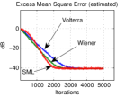
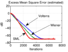
A set of two simulations, Cases I and II, on the problem of system identification, with $K=2$ and $M=10$, were run. The signal $d(i)$ was an SML plant plus additive zero-mean Gaussian noise with variance $\sigma_{n}^{2}$ (see (16)). The input signal was drawn from a zero-mean Gaussian distribuition with unitary variance, collected in the vector $u_{i}$ with a delay-line structure. In Case I, we chose $\sigma_{n}^{2}=10^{-3}$ and in Case II, $\sigma_{n}^{2}=10^{-6}$. In each case, the algorithm was run through 7000 iterations and the curves were averaged through 1000 realizations. The resulting Excess Mean Square Error (EMSE) curves (calculated as $\mathbb{E}|\mathbf{u}^{\otimes 2}(h_{1}\otimes h_{2}-\mathbf{w}[i-1])|^{2}$) are present in Figs. 2a and 2b. Plotted together on the graph are the curves for the Volterra-LMS and the Wiener-LMS, designed for the Gaussian vector $\mathbf{u}$, as described in [1]. In those algorithms, we chose $\mu$ so to get an approximately equal steady-state EMSE.

(a) Case I: Algorithms identifying an order 2 SML plant.

(b) Case II: Same as Case I; higher SNR.

(c) Case III: Algorithms identifying a different order 2 SML plant.

(d) Case IV: Algorithms identifying an order 3 SML plant.

(e) Case V: Various filters identifying a smooth plant.

(f) Case VI: Parallel cascade and SML.

Figure 2: Curves of the MSE and ESME showing the performance of the SML algorithm against other polynomial algorithms.

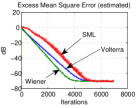
For Case III we have used a different SML plant. We had $\sigma_{n}^{2}=10^{-6}$. $\mu$ was again chosen to equalize the steady-state EMSE. The rest of the parameters remained the same.

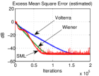
The algorithm was also made to run with $K=3$, which makes Case IV. We had $M=10$ and 200,000 iterations, averaged through 10,000 realizations. We compare the results with the Volterra-LMS and the Wiener-LMS with parameters that equalize the steady-state EMSE. The resulting curves are presented in Fig. 2d. The variance of the additive noise was chosen as $\sigma_{n}^{2}=10^{-3}$.

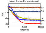
Case V compares the SML-LMS with some relevant LMS-like polynomial algorithms from the literature. Fig. 2e shows the Power Filter (PF) [12], Simplified Volterra (SV) [13, 14], Sparse Interpolated Volterra (IV) [5, 6], the regular Volterra filter and the SML. The task was to identify a smooth, non-SML, order 2 Volterra plant with $M=21$. This was averaged through 1000 realizations.

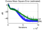
Case VI shows a simulation against another filter, the Parallel Cascade Filter (CF) [15]—single branch and LMS version. This algorithm is similar to the SML for $K\leq 2$, so we simulated them in $K=3$, where they are clearly dissimilar. We identify the same plant as Case IV, with $M=10$, through 1000 realizations. The results are on Fig. 2f.

For both Cases V and VI the additive noise variance was $10^{-3}$. The parameters were adjusted to provide approximately the same convergence rate.

A description of all the plants is available with the on-line materials in the file plants.pdf.

VI Discussion

Cases I and II clearly show the system converging to an EMSE of approximately $-40$ dB and $-70$ dB, respectively. On both Figs. 2a and 2b, we can see the SML-LMS running slower through the first 500 iterations, then it speeds up and catches up with—and eventually overtake—the others. Both the Volterra and Wiener models assume $O\left(M+K-1\choose K\right)$ operations per iteration, while the SML only $O(KM+K^{2})$. Although it is natural that the SML algorithm is better at identifying SML plants, it does it faster and with far fewer arithmetic operations.

Note that the SML algorithm presents richer dynamics compared to the other algorithms—something that will be studied in following publications. Case III, in Fig. 2c, for example, shows that its behavior does not depend only on statistics of the regressor $u_{i}$—in fact, it is also influenced by the plant to be identified. A source of these effects can be hypothesised as due to the $y_{s}(i)$ factors in (21).

Case IV, in Fig. 2d, shows that the algorithm also converges for $K=3$ and that it has the aforementioned initial irregular convergence rate, here appearing in a more evident way.

Case V shows that the algorithm is competitive, even in a non-SML plant—as long as this plant is correlated enough. The PF used 21 coefficients, the SV used 66, the IV used 60, Volterra used 231 and SML 42. This is another result that shows the computational simplicity of the SML.

Case VI shows two similar filters, in the sense that they are formed through the product of others. SML is a product of three linear filters, with a total of 30 coefficients, and CF is a product of a linear filter with a second order Volterra filter, with 66 coefficients. In the task of identifying an SML plant, they show similar behavior, with the SML being slightly better—at half the complexity.

VII Conclusion

Through the use of a Kronecker representation, we have developed the cost function for the SML model. From this function its gradient was derived motivating a new LMS-like nonlinear adaptive algorithm. It has very low computational complexity—an exponential reduction when compared to te Volterra series—and a competitive mean-square performance in a variety of cases, but also some other unusual behavior.

Finally, the SML algorithm, just like the Parallel Cascade Filter [15], allows the extension for models of greater rank. This path will be pursued in future publications.

Appendix A Proof of the Gradient Formula

Through (7) and (8), one can interpret (14) as a tensor equation, in the sense that we can index the matrices as

$$(R_{u^{K}})^{i_{1},\dotsc,i_{K}}_{j_{1},\dotsc,j_{K}}=\mathbb{E}(\mathbf{u}^{\otimes K*}\mathbf{u}^{\otimes K})^{i_{1},\dotsc,i_{K}}_{j_{1},\dotsc,j_{K}}$$

$$\text{and}\quad(R_{u^{K}d})_{j_{1},\dotsc,j_{K}}=\mathbb{E}(\mathbf{u}^{\otimes K}\mathbf{d})_{j_{1},\dotsc,j_{K}}$$

so to write

$$R_{u^{K}d}w=\sum_{j_{1},\dotsc,j_{K}}(R_{u^{K}d})_{j_{1},\dotsc,j_{K}}\prod_{\ell}(w_{\ell})^{j_{\ell}},$$

where $(w_{\ell})^{j_{\ell}}$ is the $j_{\ell}$-th coordinate of $w_{\ell}$, and

$$w^{*}R_{u^{K}}w=\sum_{\begin{subarray}{c}i_{1},\dotsc,i_{K}\\ j_{1},\dotsc,j_{K}\end{subarray}}\prod_{p}(w_{p})^{i_{p}*}(R_{u^{K}})^{i_{1},\dotsc,i_{K}}_{j_{1},\dotsc,j_{K}}\prod_{\ell}(w_{\ell})^{j_{\ell}}.$$

The other terms from (14) involve only the conjugates of the entries of $w$, so they became to zero[8].

The gradient over the vector $w_{s}$ is given by the derivatives over each of its components:

$$\frac{\partial(R_{u^{K}d})w}{\partial(w_{s})^{j_{q}}}=\sum_{j_{1},\dotsc,j_{K}}(R_{u^{K}d})_{j_{1},\dotsc,j_{K}}\prod_{\ell\neq s}(w_{\ell})^{j_{\ell}}\delta^{j_{s}}_{j_{q}}.$$

$\delta^{i}_{j}$ is the Kronecker delta and also the representation of the identity matrix. In the above expression, the delta—the identity—takes the place of the factor $(w_{s})^{j_{s}}$. This observation leads directly to

$$\nabla_{w_{s}}(R_{u^{K}d}w)=R_{u^{K}d}(w_{1}\otimes\dotsb\otimes\widehat{w_{s}}\otimes\dotsb\otimes w_{K}).$$

For $w^{*}R_{u^{K}}w$, we have, remembering we do not derivate the conjugates [8],

$$\frac{\partial(w^{*}R_{u^{K}}w)}{\partial(w_{s})^{j_{q}}}=\sum_{\begin{subarray}{c}i_{1},\dotsc,i_{K}\\ j_{1},\dotsc,j_{K}\end{subarray}}\prod_{p}(w_{p}^{*})_{i_{p}}(R_{u^{K}})^{i_{1},\dotsc,i_{K}}_{j_{1},\dotsc,j_{K}}\prod_{\ell\neq s}(w_{\ell})^{j_{\ell}}\delta^{j_{s}}_{j_{q}}.$$

Under the same argument,

$$\nabla_{w_{s}}(wR_{u^{K}}w^{*})=w^{*}R_{u^{K}}(w_{1}\otimes\dotsb\otimes\widehat{w_{s}}\otimes\dotsb\otimes w_{K}).$$

Therefore, we combine those two terms to get

$$\nabla_{w_{s}}\text{MSE} =\nabla_{w_{s}}(R_{d}-w^{*}R_{u^{K}d}^{*}-R_{u^{K}d}w+w^{*}R_{u^{K}}w)$$

$$=-\nabla_{w_{s}}(R_{u^{K}d}w)+\nabla_{w_{s}}(w^{*}R_{u^{K}}w)$$

$$=[-R_{u^{K}d}+w^{*}R_{u^{K}}](w_{1}\otimes\dotsb\otimes\widehat{w_{s}}\otimes\dotsb\otimes w_{K}).$$

See pages - of plants.pdf

References

- [1] T. Ogunfunmi, Adaptive Nonlinear System Indentification: The Volterra and Wiener Model Approaches. Secaucus, NJ, USA: Springer-Verlag New York, Inc., 2006.
- [2] V. Mathews, “Adaptive polynomial filters,” Signal Processing Magazine, IEEE, vol. 8, no. 3, pp. 10–26, July 1991.
- [3] S. Boyd, L. O. Chua, and C. A. Desoer, “Adaptive polynomial filters,” IMA Journal of Mathematical Control and Information, Oxford University Press, vol. 1, no. 3, pp. 243–282, 1984.
- [4] R. Nowak and B. Van Veen, “Tensor product basis approximations for volterra filters,” Signal Processing, IEEE Transactions on, vol. 44, no. 1, pp. 36–50, Jan 1996.
- [5] E. Batista, O. J. Tobias, and R. Seara, “A fully lms adaptive interpolated volterra structure,” in Acoustics, Speech and Signal Processing, 2008. ICASSP 2008. IEEE International Conference on, March 2008, pp. 3613–3616.
- [6] E. Batista, O. Tobias, and R. Seara, “A sparse-interpolated scheme for implementing adaptive volterra filters,” Signal Processing, IEEE Transactions on, vol. 58, no. 4, pp. 2022–2035, April 2010.
- [7] T. Andre, R. Nowak, and B. Van Veen, “Low rank estimation of higher order statistics,” in Acoustics, Speech, and Signal Processing, 1996. ICASSP-96. Conference Proceedings., 1996 IEEE International Conference on, vol. 5, May 1996, pp. 3026–308a vol. 5.
- [8] A. H. Sayed, Adaptive Filters. Wiley-IEEE Press, 2008.
- [9] J. Brewer, “Kronecker products and matrix calculus in system theory,” Circuits and Systems, IEEE Transactions on, vol. 25, no. 9, pp. 772–781, Sep 1978.
- [10] S. Roman, Advanced Linear Algebra. Springer, 2007.
- [11] W. Greub, Multilinear Algebra, ser. Universitext. Springer New York, 2012.
- [12] F. Kuech, A. Mitnacht, and W. Kellermann, “Nonlinear acoustic echo cancellation using adaptive orthogonalized power filters,” in Acoustics, Speech, and Signal Processing, 2005. Proceedings. (ICASSP ’05). IEEE International Conference on, vol. 3, March 2005, pp. iii/105–iii/108 Vol. 3.
- [13] A. Fermo, A. Carini, and G. L. Sicuranza, “Low-complexity nonlinear adaptive filters for acoustic echo cancellation in gsm handset receivers,” European Transactions on Telecommunications, vol. 14, no. 2, pp. 161–169, 2003. [Online]. Available: http://dx.doi.org/10.1002/ett.908
- [14] ——, “Simplified volterra filters for acoustic echo cancellation in gsm receivers,” in Signal Processing Conference, 2000 10th European, Sept 2000, pp. 1–4.
- [15] T. M. Panicker, V. J. Mathews, and G. L. Sicuranza, “Adaptive parallel-cascade truncated volterra filters,” IEEE Transactions on Signal Processing, vol. 46, no. 10, pp. 2664–2673, Oct 1998.