A targeted spectral interpolation algorithm for the detection of continuous gravitational waves

Abstract

We present an improved method of targeting continuous gravitational-wave signals in data from the LIGO and Virgo detectors with a higher efficiency than the time-domain Bayesian pipeline used in many previous searches. Our spectral interpolation algorithm, SplInter, removes the intrinsic phase evolution of the signal from source rotation and relative detector motion. We do this in the frequency domain and generate a time series containing only variations in the signal due to the antenna pattern. Although less flexible than the classic heterodyne approach, SplInter allows for rapid analysis of putative signals from isolated (and some binary) pulsars, and efficient follow-up searches for candidate signals generated by other search methods. The computational saving over the heterodyne approach can be many orders of magnitude, up to a factor of around fifty thousand in some cases, with a minimal impact on overall sensitivity for most targets.

1 Introduction

Rapidly rotating neutron stars are promising sources of long-lived gravitational-wave signals and one of the key science targets of the LIGO and Virgo Scientific Collaborations [1]. The full parameter space for these signals is too large for simple coherent methods to be employed on timescales longer than a few days, so a range of more specific methods have been developed to explore specific regions of the space to different depths [2]. Known radio and X-ray pulsars comprise an important class of potential gravitational-wave source and three analysis pipelines have been specifically developed to exploit the known rotational phase evolution of these targets [3, 4, 5]. These targeted pipelines are fully-coherent over arbitrary lengths of time, tracking the predicted gravitational signal based on electromagnetic observations. They perform the deepest gravitational wave searches in the field and all three use both time and frequency domain techniques to reduce the data at relatively low computational cost. However, as these pipelines are now being applied more widely to candidate sources identified by other searches there is significant benefit in reducing the cost still further. Two of these (the Bayesian targeted and $\mathcal{G}$ statistic [3, 5] pipelines), rely on data from a carefully implemented, but slow, heterodyne step developed by Dupuis and Woan [2, 3, 6, 7] that allows the data to be sampled at a much lower rate than is generated by the detector (from $\sim 16$  kHz to usually one sample per minute). Although we believe this exact solution is still the best way to approach high-value targets, short-period binaries and targets close to spectral lines (such as the Crab pulsar), when certain approximations are valid the step can be performed more efficiently for many other targets using fast fourier transform (FFT) methods. We therefore present an efficient method for down-sampling gravitational wave data and removing the effects of detector motion with respect to the source based on FFTs. Similar spectral methods have been used widely in the field for many years, and indeed form the basis of the $\mathcal{F}$-statistic search methods [8] which are ubiquitous. Our version of spectral interpolation, SplInter, is designed as a more efficient replacement for the heterodyne algorithm in certain situations. As we will show, our algorithm’s large computational costs savings and very small sensitivity losses (when certain signal assumptions are valid) mean that it can be quickly and easily applied to a large number of targets, e.g. if following up large numbers of potential candidate signals from blind all-sky searches.

In section 3 we show how to calculate the down-sampled data streams using this method. In section 4 we confirm the equivalence of these streams to those from the heterodyne method, and assess the improvement in computational efficiency offered by SplInter.

The continuous gravitational wave strain signal in the output of a detector depends on the source emission mechanism and the source/detector geometry, but for the purposes of this analysis we assume it to be quasi-sinusoidal, with the form

$$h(T)=A(T)\mathrm{\rm e}^{\rmi\Phi(T)}+A^{*}(T)\mathrm{\rm e}^{-\rmi\Phi(T)},$$ (1)

where $A(T)$ contains both the antenna response pattern and source amplitude parameters. $\Phi(T)$ is the apparent phase evolution of the signal due to source rotation and $T$ is the time in a suitable inertial frame (see below). For example in the case of a triaxial neutron star rotating about a principle axis, emitting gravitational waves at twice the rotation frequency, $A$ has the form [3]

$$A(T)=\frac{1}{4}F_{+}(T;\psi)h_{0}(1+\cos^{2}\iota)-\frac{\rmi}{2}F_{\times}(T;\psi)h_{0}\cos\iota,$$ (2)

where $\iota$ is the inclination angle between the source rotation axis and the line of sight from the detector to the source, $\psi$ is the gravitational wave polarisation angle and $h_{0}$ is the wave amplitude. $F_{+}$ and $F_{\times}$ are the antenna pattern responses to plus and cross polarisations respectively. The evolution of $\Phi(T)$ depends on the intrinsic rotational evolution of the neutron star, defined by its frequency and frequency derivatives $f^{(0),(1),(2)...}_{\textrm{\footnotesize rotation}}$. Over short timescales, the time-dependence of $h(T)$ is dominated by this phase term, expanded as

$$\Phi(T)=\Phi_{0}+2\pi\sum_{l=0}\frac{f^{(l)}(T-T_{0})^{l+1}}{(l+1)!},$$ (3)

where $f^{(l)}$ is the $l^{\rm th}$ time derivative of the gravitational wave frequency (note that these are twice the rotation values for the $l=m=2$ harmonic of a non-precessing, triaxial neutron star), $T_{0}$ is the epoch at which ${\Phi(T_{0})=\Phi_{0}}$. The $f^{(l)}$ values are derived from radio, X-ray, or $\gamma$-ray pulse times-of-arrival, preferably from data spanning the same analysis period as the gravitational wave search in question.

The rotational and orbital motions of the Earth put the detector in a non-inertial rest frame, but for a given source position on the sky we can relate the topocentric signal arrival times at the detector, $t^{\prime}$, to those in the source’s frame of reference by

$$T=t^{\prime}+\delta(t^{\prime}),$$ (4)

where $\delta(t^{\prime})$ comprises four time-delay terms [3]:

$$\delta(t^{\prime})=\Delta_{\textrm{R}\odot}+\Delta_{\textrm{S}\odot}+\Delta_{\textrm{E}\odot}+\Delta_{\textrm{\footnotesize Binary}}.$$ (5)

The Roemer delay $\Delta_{\textrm{R}\odot}$ is the dominant term; it is the Euclidian difference in time taken for the signal to arrive at the detector and the solar system barycentre (SSB). $\Delta_{\textrm{S}\odot}$ is the Shapiro delay, caused by the bending of spacetime near to massive bodies, which in the case of an Earth-based detector is dominated by the Sun’s contribution. The Einstein delay $\Delta_{\textrm{E}\odot}$ combines the effects of special and general relativistic time dilation due to motion and the presence of massive bodies. All of these terms vary slowly over the course of a year, and by small amounts over the course of a day, and as such can be considered as changing only linearly over the half-hour intervals we will consider shortly. These effects can be addressed in a number of ways, including resampling [9] or heterodyning [3] the data. $\Delta_{\rm Binary}$ however can vary more quickly, on the timescale of the period of binary motion, this is an additional all-encompassing term that combines the Roemer, Shapiro and Einstein delays caused by the source’s non-inertial motion, should it be in a binary system. In terms of the topocentric time we now have

$$\Phi(t^{\prime})=\phi_{0}+2\pi\sum_{l=0}\frac{f^{(l)}(t^{\prime}+\delta(t)-t_{0})^{l+1}}{(l+1)!},$$ (6)

where $t_{0}$ is the time at which $\Phi(t_{0}-\delta)=\phi_{0}$.

Any difference in the assumed and actual phase evolution would introduce a residual phase evolution and a reduction in final search sensitivity. Typically, known radio and X-ray pulsars are timed sufficiently well for these effects to be negligible, but they can be included straightforwardly in the subsequent parameter estimation stages of a search. Once we have corrected for this known phase variation the only remaining time-dependence in Equation 1 is from $A(t)$, which evolves as the antenna pattern sweeps over the source in a sidereal day. We can therefore sample the data at a much reduced rate, limited only by the changing antenna pattern, provided that we still capture this. The original heterodyne pipeline achieves phase correction by multiplying the strain time series $s(t^{\prime})$ (where we use the notation of [3] that $s(t^{\prime})=h(t^{\prime})+n(t^{\prime})$, where $h(t^{\prime})$ is the signal from Equation 1 and $n(t^{\prime})$ is Gaussian noise) by $\exp[-\rmi\phi(t^{\prime})]$, where $\phi(t^{\prime})=\Phi(t^{\prime})-\phi_{0}$, effectively shifting the signal frequency to zero and leaving $A(t)$ as the only time-dependent term. After applying a low-pass filter (conventionally with a time constant of 1 minute) we average over $M$ data samples to obtain a down-sampled time series of the form

$$B_{K}=\frac{1}{M}\sum\limits_{j=1}^{M}s(t^{\prime}_{j})\exp[-\rmi\phi(t^{\prime}_{j})],$$ (7)

where $M$ is the number of raw data samples contributing to $B_{K}$ (following [3] this is often chosen to give one sample per minute), and $K$ is the time index for the resulting time series. We model this as a combination of a signal term $y_{K}=A(t_{K})\exp(\rmi\phi_{0})$ and, appropriately over the narrow bands considered here, white Gaussian noise $n_{K}\sim N(0,\sigma_{K}^{2})$

$$B_{K}=y_{K}+n_{K}.$$ (8)

$\sigma_{K}$ is modelled as constant over short timescales, and is related to the original time-series noise $\sigma_{T}$ by

$$\sigma_{K}^{2}=\frac{\sigma_{T}^{2}}{M}=\frac{\sigma_{T}^{2}}{r\Delta t},$$ (9)

where $r$ is the original sample rate and $\Delta t$ is the down-sampled period.

2 Formulation in the frequency domain

We can consider a similar analysis in the frequency domain. The Fourier transform of a signal $h(t^{\prime})$ limited in duration to $\Delta t$ centred on a time ($t_{k}-t_{0}$) is

$$H_{k}(f)=\int\limits^{t_{k}-t_{0}+\Delta t/2}_{t_{k}-t_{0}-\Delta t/2}\left[A(t^{\prime})\mathrm{\rm e}^{\rmi\Phi(t^{\prime})}+A^{*}(t^{\prime})\mathrm{\rm e}^{-\rmi\Phi(t^{\prime})}\right]\exp\left[-2\pi\rmi f(t^{\prime}-t_{0}-t_{k}+\Delta t/2)\right]\,{\mathrm{d}}t^{\prime}.\\$$

In this Fourier-based version, $t_{k}$ become the time-stamps of a series similar to the $t_{K}$ series defined above, with $H_{k}(f_{\rm signal})$ playing the role of $y_{K}$. However, we now use $k$ rather than $K$ as the index to highlight that the two sampling rates need not be (and indeed usually are not) the same. $t_{0}$ is (again) the reference epoch of our timing solution.

We now consider $\phi(t^{\prime})$, the time-dependent part of $\Phi(t^{\prime})$, and use a time coordinate $t$ with its origin at the mid-point of the data under consideration i.e., ${t^{\prime}\rightarrow t=t^{\prime}-t_{k}+t_{0}}$. Importantly, the time-delay correction term $\delta(t)$ in (5) will vary slightly over the time $\Delta t$. We approximate these changes in the arrival time to first order in $t$, defining $\delta_{k}=\delta(t_{k})$ and $\dot{\delta}_{k}=\frac{\,{\mathrm{d}}}{\,{\mathrm{d}}t}\delta(t_{k})$, such that for the duration of the data ${\delta(t)\approx\delta_{k}+\dot{\delta}_{k}t}$. Equation 6 now becomes

$$\phi(t)\approx 2\pi\sum_{l=0}\frac{f^{(l)}\left[t(1+\dot{\delta}_{k})+t_{k}-t_{0}+\delta_{k}\right]^{l+1}}{(l+1)!}.$$

To second order in $t$

$$\phi(t)\approx\phi_{k}+2\pi f_{k}t+\pi\dot{f_{k}}t^{2},$$ (10)

where

$$\phi_{k}\mathrel{\mathop{:}}=2\pi\sum_{l=0}\frac{f^{(l)}(t_{k}-t_{0}+\delta_{k})^{l+1}}{(l+1)!},$$ (11)

and

$$f_{k}\mathrel{\mathop{:}}=(1+\dot{\delta}_{k})\sum_{l=0}\frac{f^{(l)}(t_{k}-t_{0}+\delta_{k})^{l}}{l!}.$$ (12)

We also approximate $\dot{f}_{k}$ as

$$\dot{f}_{k}=\frac{f_{\rm end}-f_{\rm start}}{\Delta t}.$$ (13)

where

$$f_{\rm start}=\left[1+\frac{\,{\mathrm{d}}}{\,{\mathrm{d}}t}\delta\left(t_{k}-\frac{\Delta t}{2}\right)\right]\sum_{l=0}\frac{f^{(l)}\left[t_{k}-\frac{\Delta t}{2}-t_{0}+\delta\left(t_{k}-\frac{\Delta t}{2}\right)\right]^{l}}{l!}.$$ (14)

and

$$f_{\rm end}=\left[1+\frac{\,{\mathrm{d}}}{\,{\mathrm{d}}t}\delta\left(t_{k}+\frac{\Delta t}{2}\right)\right]\sum_{l=0}\frac{f^{(l)}\left[t_{k}+\frac{\Delta t}{2}-t_{0}+\delta\left(t_{k}+\frac{\Delta t}{2}\right)\right]^{l}}{l!}.$$ (15)

We assume the signal amplitude and antenna pattern contributions to $A(t)$ are approximately constant on timescales of a small fraction of a day, so when $\Delta t$ is small we can replace $A(t)$ above with $A(t_{k})$. Having defined ${y_{k}:=A(t_{k})\mathrm{\rm e}^{\rmi\phi_{0}}}$ we can therefore write, using these approximations,

$$H_{k}(f)\approx\mathrm{\rm e}^{-\rmi\pi f\Delta t}\int\limits^{\Delta t/2}_{-\Delta t/2}\left[y_{k}\mathrm{\rm e}^{\rmi\phi(t)}+y_{k}^{*}\mathrm{\rm e}^{-\rmi\phi(t)}\right]\mathrm{\rm e}^{-2\pi\rmi ft}\,{\mathrm{d}}t.$$ (16)

This is the Fourier transform which will be considered in the following models.

2.1 The form of the signal in a short transform

Our signal is quasi-sinusoidal, but with amplitude and phase varying slowly as the source moves though the antenna pattern, and with changes in delay and doppler shift as well as intrinsic variations in the source spin rate. To first order in $f$, using $H_{k}(f)$ from (16) and $\phi(t)$ from (10) we have

$$H_{k}(f)\approx y_{k} \mathrm{\rm e}^{\rmi\phi_{k}-\rmi\pi f\Delta t}\int\limits^{\Delta t/2}_{-\Delta t/2}\exp\left[2\pi\rmi(f_{k}-f)t+\rmi\pi\dot{f_{k}}t^{2}\right]\,{\mathrm{d}}t$$ (17)

$$+y_{k}^{*}\mathrm{\rm e}^{-\rmi\phi_{k}-\rmi\pi f\Delta t}\int\limits^{\Delta t/2}_{-\Delta t/2}\exp\left[-2\pi\rmi(f_{k}+f)t-\rmi\pi\dot{f_{k}}t^{2}\right]\,{\mathrm{d}}t.$$

These expressions are not strictly analytic due to the $t^{2}$ phase-dependency of the exponent, but are forms of the familiar Fresnel integral. The limiting form, when $\dot{f_{k}}$ is small, is just the Fourier transform of a time-limited sinusoid, so we will consider this as a special case below.

2.1.1 The sinc approximation, $\dot{f_{k}}=0$

The contribution of the intrinsic spin-down of the source, $f^{(1)}$, to the overall $\dot{f}$ is generally negligible over the course of a single transform (maybe lasting minutes to hours) and the change in frequency due to this component will be much smaller than the frequency resolution. For example the Crab pulsar, which has an unusually large spin-down of $f^{(1)}=7.4\times 10^{-10}$ Hz s^-1 [10, 11], will change in frequency by only $\Delta f=1.3\times 10^{-6}$ Hz over 30 minutes, which is $0.1\%$ of the width of a frequency bin. Instead, $\dot{f}_{k}$ is dominated by the $\dot{\delta}_{k}$ term caused by the orbital motions of the source and observer. The spin and orbital motion of the observer are also usually negligible over $\sim 1$ h, so for a source that is not in a binary system we can assume $\dot{f}_{k}=0$ for the duration of the integral, so that

$$H_{k}(f) \approx y_{k}\mathrm{\rm e}^{\rmi\phi_{k}-\rmi\pi f\Delta t}\int\limits^{\Delta t/2}_{-\Delta t/2}\exp\left[2\pi\rmi(f_{k}-f)t\right]\,{\mathrm{d}}t$$

$$\qquad+y_{k}^{*}\mathrm{\rm e}^{-\rmi\phi_{k}-\rmi\pi f\Delta t}\int\limits^{\Delta t/2}_{-\Delta t/2}\exp\left[-2\pi\rmi(f_{k}+f)t\right]\,{\mathrm{d}}t$$

$$\approx y_{k}\Delta t\exp\left[\rmi\phi_{k}-\rmi\pi f\Delta t\right]\mathop{\mathrm{sinc}}\nolimits\left[\pi(f_{k}-f)\Delta t\right]$$

$$\qquad+y_{k}^{*}\Delta t\exp\left[-\rmi\phi_{k}-\rmi\pi f\Delta t\right]\mathop{\mathrm{sinc}}\nolimits\left[\pi(f_{k}+f)\Delta t\right],$$ (19)

where we use the convention

$$\mathop{\mathrm{sinc}}\nolimits x\mathrel{\mathop{:}}=\frac{\sin x}{x}.$$ (20)

Close to the signal frequency (i.e., when $f\simeq f_{k}$)

$$\mathop{\mathrm{sinc}}\nolimits\left[\pi(f_{k}-f)\Delta t\right]\gg\mathop{\mathrm{sinc}}\nolimits\left[\pi(f_{k}+f)\Delta t\right],$$ (21)

so we can remove the second term in (19) to give

$$H_{k}(f)\approx y_{k}\Delta t\exp\left[\rmi\phi_{k}-\rmi\pi f\Delta t\right]\mathop{\mathrm{sinc}}\nolimits\left[\pi(f_{k}-f)\Delta t\right].$$ (22)

We will refer to this below as the sinc approximation.

2.1.2 The Fresnel approximation

If $\dot{f}_{k}$ is non-negligible then we can still approximate the form of $H_{k}(f)$ through a numerical integration. Such circumstances would occur if the doppler-shifted frequency was evolving significantly on timescales of $\Delta t$ due to the orbital motion of the source or observer. If the rate of change of signal frequency is a constant, i.e. $\ddot{f}_{k}=0$, we would expect the signal to appear as a ‘Fresnel’ pattern in the Fourier transform, characterised by the quadratic evolution of phase with time. Fresnel Integrals have been studied extensively, and there are good algorithms for fairly rapid calculation [12]. They comprise a pair of functions defined as [13]

$$\mathcal{C}[w]:=\int\limits_{0}^{w}\cos\left(\frac{\pi x^{2}}{2}\right)\,{\mathrm{d}}x$$ (23)

and

$$\mathcal{S}[w]:=\int\limits_{0}^{w}\sin\left(\frac{\pi x^{2}}{2}\right)\,{\mathrm{d}}x.$$ (24)

In terms of these integral functions, (17) becomes

$$H_{k}(f)\approx\frac{y_{k}}{2\sqrt{2|\dot{f}_{k}|}}\exp(\rmi\Delta\phi)\bigg{\{}\mathcal{C}[w_{\rm end}]+\rmi\frac{\dot{f}_{k}}{|\dot{f}_{k}|}\mathcal{S}[w_{\rm end}]-\mathcal{C}[w_{\rm start}]-\rmi\frac{\dot{f}_{k}}{|\dot{f}_{k}|}\mathcal{S}[w_{\rm start}]\bigg{\}},$$ (25)

where

$$\Delta\phi=\phi_{k}-\pi f\Delta t+\pi\frac{\dot{f}_{k}\Delta t^{2}}{2}-\frac{\pi}{\dot{f}_{k}}\left(f_{k}+\frac{\dot{f}_{k}\Delta t}{2}-f\right)^{2},$$ (26)

$$w_{\rm end}=\frac{\sqrt{2|\dot{f}_{k}|}}{\dot{f}_{k}}\left(f_{k}-f+\frac{\dot{f}_{k}\Delta t}{2}\right)+\sqrt{\frac{|\dot{f}_{k}|}{2}}\Delta t$$ (27)

and

$$w_{\rm start}=\frac{\sqrt{2|\dot{f}_{k}|}}{\dot{f}_{k}}\left(f_{k}-f+\frac{\dot{f}_{k}\Delta t}{2}\right)-\sqrt{\frac{|\dot{f}_{k}|}{2}}\Delta t.$$ (28)

Here, we have again ignored the $(f+f_{k})$ term in (17), as again it is negligible in the interpolation region where $f\simeq f_{k}$.

We will refer to (25) as the Fresnel approximation to the signal Fourier transform, and we calculate the Fresnel integral terms with sufficient numerical precision using the algorithm in [12]. For small $\dot{f}_{k}$ the Fresnel approximation reduces to the sinc approximation described above. Computationally it is more expensive than the sinc approximation, however it need only be implemented during periods of time corresponding to large values of $\dot{f}_{k}$,, i.e., $|\dot{f}_{k}|\Delta t^{2}>0.1$.

3 The Spectral Interpolation algorithm

The Spectral Interpolation algorithm (SplInter) is an alternative to the time-domain heterodyne algorithm of Dupuis and Woan [3] originally developed for gravitational-wave searches targeting known pulsars. In contrast to this heterodyne algorithm, SplInter uses Fast Fourier Transform methods to generate a similarly narrow-band time series but can process multiple targets very much more efficiently and usually with an acceptable impact on overall sensitivity. Within the LIGO Scientific Collaboration a Fourier transform data format, known as ‘Short-time Fourier Transforms’ (SFTs), has been defined [14, 15] for use in a variety of continuous gravitational wave searches. These SFTs contain discrete Fourier transforms of windowed data segments that are much shorter than the duration of the experiment (usually around half an hour). Of course there is an associated computational load in creating these SFTs, but this is offset by the efficiency of the SplInter algorithm. In addition, SFTs for several types of continuous-wave search (such as [16]) can be shared with SplInter.

In the first stage of the SplInter algorithm we take a discretely-sampled Fourier transform, in the form of an SFT, and compute a value of $H_{k}$ at the instantaneous topocentric signal frequency using one of the interpolation methods described above over a small number of spectral points either side of the central topocentric frequency bin. We denote the result of this spectral interpolation $B_{k}$. In addition, we wish to calculate $\sigma_{k}$, the standard deviation of the noise on our estimate of $B_{k}$.

3.1 $B_{k}$ and $\sigma_{k}$ calculation

An SFT is of course a discrete Fourier transform, so we must interpolate between frequency bins to recover an unbiased estimate, $B_{k}$, of the signal, $y_{k}$. The interpolation is best understood in Bayesian terms: we compute the most probable value of $y_{k}$ by choosing the value that maximises its posterior probability, given the data and a model for the signal. We choose to estimate the signal and noise separately, so for the signal estimate we will marginalise over the (unknown but assumed constant) noise variance.

We start by noticing that we can express the signal Fourier transform $H_{k}(f)$ (using either the sinc or Fresnel approximation for this expression) as the product of our unknown signal amplitude, $y_{k}$ and a known signal shape function, $\mu_{k}$, defined as

$$\mu_{k}(f)\mathrel{\mathop{:}}=\frac{H_{k}(f)}{y_{k}}.$$ (29)

If the Fourier transform of the data is $S_{k}(f)$ then, writing $S_{ki}\equiv S_{k}(f_{i})$ and $\mu_{ki}\equiv\mu_{k}(f_{i})$ the likelihood of the set of data $\{S_{k}(f)\}$ given $B_{k}$, spectral noise $\sigma_{F}$ and signal shape $\mu_{k}(f)$ is

$$\,{\textrm{p}}\left(\{S_{k}(f)\}|B_{k},\sigma_{F},\{\mu_{k}(f)\}\right)=\frac{1}{(2\pi\sigma_{F}^{2})^{N}}\exp\left(-\frac{1}{2\sigma_{F}^{2}}\sum\limits_{i=1}^{N}|S_{ki}-B_{k}\mu_{ki}|^{2}\right).$$ (30)

where the sum in $i$ is over a window of $N$ frequency bins around the signal frequency for which $|\mu|$ is significantly greater than zero. Here we have assumed that the noise is uncorrelated between frequency bins and has a constant standard deviation $\sigma_{F}$. We can consider $\sigma_{F}$ as a nuisance parameter, and marginalise over it. Choosing a Jeffreys prior for $\sigma_{F}$ of ${\,{\textrm{p}}(\sigma_{F})\propto 1/\sigma_{F}}$, ${\sigma_{F}>0}$ and a uniform prior on $B_{k}$, for ${B_{k}=-\infty}$ to $\infty$ we obtain, after marginalisation, a log posterior for $B_{k}$ of

$$\log\left[\,{\textrm{p}}\left(B_{k}|\{S_{ki}\},\{\mu_{ki}\}\right)\right]\propto-N\log\left(\sum_{i}|S_{ki}-B_{k}\mu_{ki}|^{2}\right).$$ (31)

The maximum of this log posterior occurs when ${\sum_{i}|S_{ki}-B_{k}\mu_{ki}|^{2}}$ is minimised. If we differentiate with respect to $B^{*}_{k}$ and set this to be zero we get

$$\frac{\,{\mathrm{d}}}{\,{\mathrm{d}}B^{*}_{k}}\left(\sum\limits_{i}|S_{ki}-B_{k}\mu_{ki}|^{2}\right)=\frac{\,{\mathrm{d}}}{\,{\mathrm{d}}B^{*}_{k}}\sum\limits_{i}\left(S_{ki}S^{*}_{ki}-B_{k}\mu_{ki}S^{*}_{ki}-S_{ki}B^{*}_{k}\mu^{*}_{ki}+B_{k}B^{*}_{k}\mu^{*}_{ki}\mu_{ki}\right)$$

$$=\sum\limits_{i}\left(-S_{ki}\mu^{*}_{ki}+B_{k}\mu^{*}_{ki}\mu_{ki}\right)=0.$$ (32)

The most probable value of $B_{k}$ is therefore

$$B_{k}=\frac{\sum\limits_{i}[S_{ki}\mu^{*}_{ki}]}{\sum\limits_{i}[\mu^{*}_{ki}\mu_{ki}]},$$ (33)

a result that is familiar from least-squares analysis.

To estimate the variance of the noise, $\sigma_{k}^{2}$, we would ideally follow a similar route, marginalising over $B_{k}$ in (30) and maximising the posterior for $\sigma_{k}$

$$\,{\textrm{p}}(\sigma_{k}|\{S_{ki}\},\{\mu_{ki}\})_{\rm max}=\left[\int\limits_{-\infty}^{\infty}\,{\textrm{p}}(\sigma_{k}|\{S_{ki}\},\{\mu_{ki}\},B_{k})\,{\textrm{p}}(B_{k})\,{\mathrm{d}}B_{k}\right]_{\rm max}.$$ (34)

However, this integral is not analytic. We therefore choose to use our calculated value of $B_{k}$ from (33) to obtain the best estimate of $\sigma_{k}$, equivalent to using the Dirac delta function as the prior on $B_{k}$ in (34)

$$\,{\textrm{p}}(B_{k})=\delta_{D}\left(B_{k}-\frac{\sum\limits_{i}[S_{ki}\mu^{*}_{ki}]}{\sum\limits_{i}[\mu^{*}_{ki}\mu_{ki}]}\right).$$ (35)

The application of this is straightforward: we use the most probable $B_{k}$ calculated above to return best estimate of $H_{k}(f_{i})$, ${H_{\rm best}(f_{i})=B_{k}\mu(f_{i})}$. The difference between $H_{\rm best}(f_{i})$ and $S(f_{i})$ is our best estimate of the noise $N_{\rm best}(f_{i})$. We take these noise residuals around the signal frequency and then calculate their variance to give us $\sigma_{F}^{2}$.

The spectral noise variance, $\sigma_{F}^{2}$, is related to the time domain noise through Parseval’s theorem ($\sigma_{F}^{2}=\sigma_{T}^{2}\frac{2}{\Delta t^{2}r}$). Using this and (9) we get

$$\sigma_{k}^{2}=\sigma_{F}^{2}\frac{\Delta t}{2}.$$ (36)

We now have our calculated $B_{k}$ and an estimate of $\sigma_{k}$. The parameter estimation stage of the pipeline used by Dupuis and Woan [3] treated the noise variance as a nuisance parameter to be marginalised over 30-minute segments to give a Student’s $t$-likelihood for the signal. However here we use the direct estimates of $\sigma_{k}$ described above, giving a Gaussian likelihood for use in parameter estimation.

3.2 Outlier removal

The noise in gravitational-wave data contains many line features that may affect our estimates of $B_{k}$ if they are close to the source frequency. We minimise this contamination by performing three outlier removal steps. The first outlier removal routine uses the standard deviation of $S(f)$ as an initial estimate of the noise. We then multiply this standard deviation by a number (typically around ten) decided by the user and remove any $S(f)$ data points with an absolute value above this threshold. This threshold is set to be large, to remove only the strongest lines, and the five bins either side of the signal frequency are excluded from this first step.

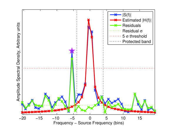
The second outlier removal step takes place after initial estimates of $B_{k}$ and $\sigma_{k}$ have been made and is shown in figure 1. By this stage we have an estimate of the noise in the frequency domain, $\sigma_{F}$, so we identify $S(f)$ data points with residual values above a threshold factor of this standard deviation. We use a factor of five in the illustrations given here. This threshold is lower than that employed in the first step, and now all but the closest $\pm 4$ data points to the signal are involved. If any data points are removed by this process $B_{k}$ and $\sigma_{F}$ are recalculated and this outlier removal step repeated to convergence.

Figure 1: An illustration of the type of outlier removed by the second outlier removal step. Shown are the best fit of the noise, the standard deviation of the residuals, the threshold for removal, and the protected band around the source frequency. The removed data point is indicated by the magenta star.

The third outlier removal step takes place after all $B_{k}$ and $\sigma_{k}$ have been calculated, and uses the noise estimates over the entire data set. We calculate the mean value of $\{\sigma_{k}\}$, $\langle\sigma\rangle$, and remove any data for which $|\mathfrak{Re}[B_{k}]|$, $|\mathfrak{Im}[B_{k}]|$ or $\sigma_{k}$ is above a threshold factor of this value. This step removes $B_{k}$ data points which are unusually noisy, but for which the noise is broadband and was not detected by the first two outlier removal steps, as shown in figure 2.

We consider it rather unlikely that our methods would accidentally veto astrophysical signals that are slightly offset from our expected frequency, as a real signal would have to be exceptionally strong to show up as significantly as the lines we are vetoing in a single SFT.

Figure 2: An illustration of the type of outlier removed by the third outlier removal step, showing the power spectra of two example SFTs. SFT1 has an unusually high low-frequency noise contribution, bleeding power into frequency channels up to around 300 Hz. For sources with signals in this lower range (such as a 90-Hz signal shown by the black line) the noise estimation for SFT1 would be large compared to that in SFT2 (a normal SFT). Sources at frequencies above $\sim 300$ Hz would be unaffected by this outlier removal.

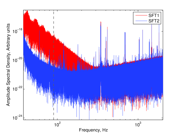
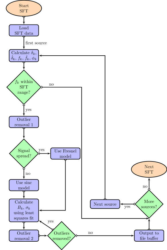
Figure 3 shows the full SplInter algorithm for a single SFT. The detector data includes data quality flags and we restrict our analysis to segments of data in ‘science mode’. The input files are therefore a science segment list and pointers to the corresponding Fourier data and a set of files defining the targets. The SplInter algorithm loops through segments, and in each segment processes each SFT according to figure 3.

Figure 3: Flowchart showing the Spectral Interpolation algorithm during each SFT. This flowchart runs for each SFT, running on a loop within each science segment, which itself is looped over. The third outlier removal is not shown, as it does not take place within this loop.

4 Testing the SplInter algorithm

We tested the SplInter algorithm against the standard heterodyne method currently employed for both accuracy and performance. The first accuracy test is described in section 4.1.1 and checked that the $B_{k/K}$ outputs from the two routines are consistent in the noiseless case. In section 4.1.3 we check that the noise estimation $\sigma_{k}$ is also accurate, and that this estimate is consistent with that estimated from the heterodyned $B_{K}$. In section 4.1.4 we perform a black-box replacement test, comparing the performance of our routines end-to-end for the analysis of hardware signal injections in LIGO S6 data [17]. Finally we test the algorithm performance in section 4.2, particularly the speed increase of SplInter compared to the heterodyne routine.

4.1 Accuracy and testing

We now compare the SplInter output, $B_{k}$, with the standard heterodyne output, $B_{K}$ (which we assume to be exact for this comparison), using the mismatch, $m$, between the two, defined as

$$m=\left|{1-\frac{\sum_{k}B_{k{\rm,Spl}}\cdot B_{k{\rm,het}}}{\sum_{k}B_{k{\rm,het}}\cdot B_{k{\rm,het}}}}\right|.$$ (37)

The mismatch is a useful indicator of how well our approximation matches the exact solution, and gives an approximate figure for the drop in SNR caused by these approximations. We define $B_{k{\rm,het}}$ as the average $B_{K}$ value over the duration of the corresponding SFT, which is equivalent to performing the heterodyne with a $\Delta t$ value of 30 minutes.

4.1.1 Recovery of noiseless signals from isolated pulsars

In the case of a noiseless signal, the heterodyne and spectral interpolation routines should, ignoring approximations, agree exactly, as $B_{k}=y_{k}$. Figures 4 and 5 show the result of applying the SplInter and heterodyne routines to noise-free data. The frames and SFTs were made using lalapps_create_pulsar_signal_frame and lalapps_MakeSFTs respectively. We see that the SplInter and heterodyne $B$-estimates agree well, and always to better than 1%. We apply a hybrid interpolation scheme here, using the sinc approximation when $\dot{f}_{k}$ is small, and the Fresnel approximation otherwise, with a changeover point at $|\dot{f}_{k}|\Delta t^{2}=0.1$ [18].

Table 1: Parameters of hardware injection pulsars 4 and 6.

$f^{(0)}$ Hz $f^{(1)}$ Hz s-1 RA Dec PULSAR4 1403.16 $-2.54\times 10^{-8}$ $18^{\rm h}\,39^{\rm m}\,57.04^{\rm s}$ $-12^{\circ}\,27^{\prime}\,59.85^{\prime\prime}$ PULSAR6 148.72 $-6.73\times 10^{-9}$ $23^{\rm h}\,55^{\rm m}\,0.23^{\rm s}$ $-65^{\circ}\,25^{\prime}\,21.45^{\prime\prime}$

Figure 4: SplInter $B_{k}$ (green/cyan/black) and fine heterodyne $B_{K}$ (red) values over one day, with amplitude on the left and phase on the right, for a noiseless signal corresponding to hardware injection PULSAR6. Below are the fractional difference between the two. SplInter values are shown using the sinc approximation (green), the Fresnel approximation (cyan) and the mixed interpolator (black), which uses the sinc approximation when $|\dot{f}_{k}|\Delta t^{2}<0.1$ and the Fresnel approximation otherwise. $m=0.0029$ for the sinc approximation, $m=0.0029$ for the mixed interpolation and $m=0.0028$ for the Fresnel approximation. The two methods are equally precise in this case, as the frequency does not significantly change during the SFT length.

Figure 5: SplInter $B_{k}$ (green/cyan/black) and fine heterodyne $B_{K}$ (red) values over one day, showing amplitude, phase and real/imaginary parts for a noiseless signal corresponding to hardware injection PULSAR4 (colours as figure 4. $|\dot{f}_{k}|$ is high for this pulsar, and the Fresnel approximation is used by the mixed interpolator to maintain accuracy. There is a significant discrepency in the real part of $B_{k}$ when using just the sinc approximation. ($m=0.0101$ for sinc, $0.0040$ for mixed and $0.0039$ for the Fresnel approximation.

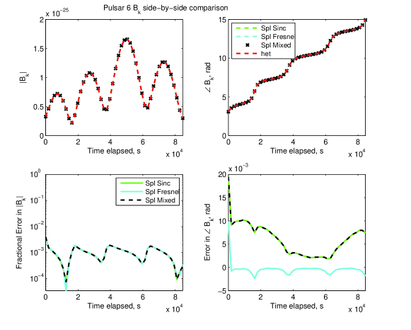
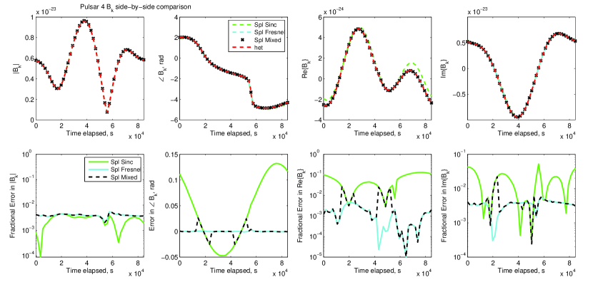
Figure 5 shows the importance of using the Fresnel rather than the sinc approximation for PULSAR4. This source has both a high frequency and a relatively low declination, leading to a large second order change in phase over the duration of the SFT.

4.1.2 Recovery of noiseless signals from binary pulsars

The signal delay for a binary pulsar contains an extra term, $\Delta_{\rm Binary}$ , in (5) from the Roemer, Shapiro and Einstein delays in the binary system itself, and this delay can introduce rapid variations in apparent frequency. Figure 6 shows which of the 97 known binary pulsars have a mismatch below 0.1 (circled) when comparing the $B_{k}$ values analysed with SplInter and heterodyne respectively. We compute the mismatch over one day if the binary period $P_{\rm b}$ is $<$1 d, over the binary period if $1<P_{\rm b}<5$ d and over 5 d if $P_{\rm b}>5$ d.

Figure 6: Binary period vs projected semi-major axis for targeted binary pulsars, indicating which binary pulsars have a small enough mismatch to be analysed using SplInter and which cannot. We include an indication of the empirical criteria we set for analysis of a target in a binary system, given in (38), for pulsars with source frequency of 10, 100 and 1000 Hz.

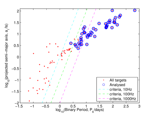
50 of these sources are in systems that show mismatches above 0.1 for SplInter, and we are therefore unable to use this method for these and maintain accuracy and sensitivity. The mismatch comes from significant high-order frequency derivatives in these pulsars over the 30 min period of the SFT. The second-order frequency derivative $\ddot{f}_{k}$ is proportional to $f^{(0)}a_{1}/P_{\rm b}^{3}$, where $a_{1}$ is the projected semi-major axis of the binary system. By considering which binary pulsars we are unable to analyse using SplInter (those not circled in figure 6), we can set an empirical upper-limit on $\ddot{f}_{k}$. When using 30 min SFTs, this limit is

$$\frac{f^{(0)}}{1\,\rm{Hz}}\frac{a_{1}}{1\,{\rm lightsecond}}\left(\frac{P_{\rm b}}{1\,{\rm day}}\right)^{-3}\lesssim 10,$$ (38)

and this limit is delineated in figure 6 for pulsars with gravitational wave frequencies of 10, 100 and 1000 Hz.

4.1.3 Noise estimation tests

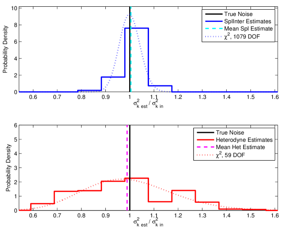
We tested noise estimation using SFTs and frames with known levels of white noise but no signal. After running the SplInter and heterodyne algorithms, we checked that the $B_{k/K}$ noise estimates were consistent with the injected value and with each other. We compared noise estimates from the SplInter routine to noise estimates from the heterodyne routine for noise data with a time-domain variance of $\sigma_{T}^{2}=1$. The estimate of the noise from the heterodyne, $\sigma_{H}$, was obtained using an average of the variance of the real and imaginary heterodyne parts over the duration of an SFT, converted into the equivalent noise value for the 30-min cadence of $B_{k}$.

We see in figure 7 that the heterodyne and SplInter noise estimates are consistent, and that both agree with the injected value of the noise and the expected distribution of these estimates. The expected distribution is a $\chi^{2}$ distribution with $n-1$ degrees of freedom, where $n$ is the number of data points used to calculate the noise estimate:

$$\frac{\sigma_{k}^{2}}{\sigma_{\rm true}^{2}}\sim\frac{\chi^{2}(n-1)}{n-1},$$ (39)

which for large $n$ approximates a normal distribution with unit mean and variance $2/(n-1)$. The heterodyne noise estimate used 30 $B_{K}$ data points from each of the real and imaginary parts of the data, leading to an expected distribution of a $\chi^{2}$ with 59 degrees of freedom, shown in the figure by the red dotted line. Here we used the spectral interpolation algorithm with a bandwidth of 0.3 Hz around the signal frequency, leading to a $\chi^{2}$ distribution on $\sigma_{k}^{2}$ with 1079 degrees of freedom (shown on the figure as a blue dotted line). One might get a marginally better noise estimate using a wider bandwidth, however the frequency dependence of the noise limits this. Additionally, there are diminishing returns in computational efficiency, and repeated use of the algorithm has found that a bandwidth of 0.3Hz is a good compromise between these considerations.

Figure 7: A histogram of standard deviation estimates of white noise from SplInter (top) and heterodyne (bottom), with the mean estimated values shown as dashed lines. Also shown is the true value of the noise (black dashed line) and the expected distributions of these values (dotted lines).

4.1.4 Full testing with hardware injections

The LSC and Virgo collaborations inject artificial signals into the detector hardware control loops to test analysis pipelines. Here we show the results of running both the heterodyne and SplInter pipelines on two hardware-injected pulsars ( ‘PULSAR4’ and ‘PULSAR6’, the parameters of which are given in table 1) in just under four months of LIGO S6 data from the Hanford detector (LHO). During this interval the LHO duty cycle was 47%, giving $\sim 5\times 10^{6}$ s of science data. With 4 months of data the injections can be recovered with a high signal-to-noise ratio, but with the posteriors retaining sufficient width to usefully assess our noise estimates. Table 2 lists the returned signal-to-noise ratios for the two pulsars using both the SplInter and heterodyne pipelines, running the latter with both a Gaussian and Student’s $t$ likelihood.

Table 2: SNRs of hardware injections 4 and 6 recovered by the two pipelines from four months of LIGO Hanford S6 strain data, calculated using the nested sampling algorithm lalapps_pulsar_parameter_estimation_nested [19]

$B_{k/K}$ algorithm SplInter heterodyne Likelihood distribution Gaussian Student’s $t$ PULSAR4 234.67 251.99 235.23 PULSAR6 16.02 17.22 17.18

We see that the SplInter results are consistent with those from the heterodyne pipeline, with SNR values around 7% below those from heterodyne. This is to be expected in real data containing segments and lines as the filtering is different in the two pipelines. Most of this drop in SNR (around 5%) is due to SplInter’s need for contiguous 30-min stretches of science data, rather than the 60 s stretches used by the heterodyne pipeline.

Figures 8 and 9 show the posterior distributions of the four source parameters determined in targeted searches, $h_{0}$, $\phi_{0}$, $\cos\iota$ and $\psi$.

Figure 8: Posterior distributions on $h_{0}$, $\phi_{0}$, $\cos\iota$ and $\psi$ for hardware injection PULSAR4 using four months of LHO S6 data. The blue dotted line shows posteriors made using SplInter for the calculation of $B_{k/K}$, and the red dashed and green solid lines show the heterodyne algorithm with Gaussian and Student’s $t$-likelihood distribution respectively. The vertical black line shows the injection value, which is slightly offset from the recovered signal due to calibration uncertainties.

Figure 9: Posterior distributions on $h_{0}$, $\phi_{0}$, $\cos\iota$ and $\psi$ for hardware injection PULSAR6 using four months of LHO S6 data. Colour scheme as in figure 8.

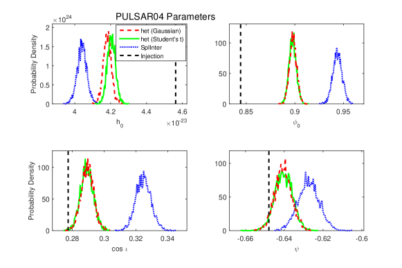
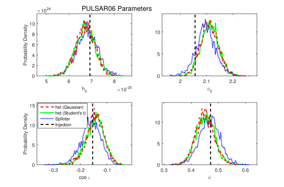
Again, in this example the posteriors generated by the two pipelines show sufficiently good agreement to allow the SplInter pipeline to replace the heterodyne pipeline without a systematically significant impact on overall performance. In figure 8 the discrepancies between the injected values and the recovered posteriors are within the range expected due to calibration uncertainties, and the discrepancies between the heterodyne and SplInter data are small enough to demonstrate that SplInter is a viable replacement for most targets, but that the heterodyne method should be retained for more accurate analysis.

4.2 Speed testing

The purpose of SplInter is to decrease the computational cost of targeted searches without significantly affecting sensitivity. We now consider the speed of SplInter in comparison with the heterodyne algorithm. The fundamental speed increase comes from the fact that we do not require the entire data bandwidth for our estimate of $B_{k}$. SplInter only requires a small frequency band of less than 1 Hz, whereas the heterodyne algorithm initially starts with a dataset containing the equivalent of 16384 Hz. In addition to this, we can analyse the sources in parallel for each SFT, reducing overall file input/output time when alaysing multiple sources.

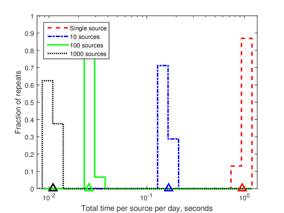
It is simplest to compare the total algorithm time taken per source, as the heterodyne algorithm simply takes the sources one at a time. However the SplInter execution time is not linear in the number of sources, so we also compare the total time per source, for one, ten, one hundred and one thousand sources at a time. These tests use the mixed interpolation scheme, so that we gain accurate timing results, including the occasional use of the Fresnel approximation.

Table 3 and figure 10 show the amount of time taken to analyse the sources for a day of continuous data using both the heterodyne and SplInter routines. Table 3 also shows the computational improvement in CPU hours per source per hour of data. We see that the SplInter routine can improve the computational efficiency of the $B_{k/K}$ calculation by up to two orders of magnitude for single source input, and four orders of magnitude if we use multiple source input. These analyses were performed on the atlas computing cluster at the Albert Einstein Institute, Hannover.

Figure 10: Histograms of the average time taken to analyse sources for a day of continuous data for the SplInter algorithm. The time taken by the heterodyne algorithm is 5.0$\times 10^{2}$ seconds per day per source, which would be over two orders of magnitude past the right hand limit of this figure. The different coloured histograms show the different number of sources used in each analysis. The horizontal axis markers denote the mean values for these times for the different numbers of sources.

Table 3: Median time taken to analyse sources for a day of data using heterodyne and Spectral Interpolation in seconds and CPU core hours per number of sources per hour of data for each interferometer.

Heterodyne SplInter Sources 1 1 10 100 1000 Time/day (s) 5.0$\times 10^{2}$ 1.0 1.7 2.5 10.9 CPUh/N/h 5.8$\times 10^{-3}$ 1.1$\times 10^{-5}$ 1.9$\times 10^{-6}$ 2.9$\times 10^{-7}$ 1.2$\times 10^{-7}$

The improvement in computational efficiency is not just limited to the $B_{k}$ calculation stage. The lower cadence of the SplInter $B_{k}$ data results in fewer data points containing a similar amount of information and hence faster calculations at the parameter estimation stage. This does however come with a cost: SplInter requires contiguous 30-min periods and lacks the flexibility of the heterodyne code in that respect.

5 Discussion

We have introduced SplInter, a new spectral interpolation method of calculating the down-sampled complex amplitude of a continuous wave signal with relative motion and source rotation effects removed. We have shown that this algorithm improves the computational efficiency of this part of the Bayesian targeted and $\mathcal{G}$-statistic pipelines by up to four orders of magnitude, and have explained how using longer time steps for $B_{k/K}$ with an estimate of the noise has a knock-on effect of improving computational speed in the parameter estimation stage. We have also shown that the SplInter routine performs well in comparison to the heterodyne routine in most cases, and that there is no significant drop in the recovered SNR. The increase in computational efficiency means that the search is a viable rapid follow-up pipeline for all-sky or directed search candidates, and preliminary results for this secondary use are in [18]. This method has been used in dual-harmonic searches for gravitational waves from spinning neutron stars [20], in which the Spectral Interpolation algorithm was found to improve the upper limit on J1748$-$2446ac by a factor of 1.7 compared to [2] by the use of the line removal routine.

Tests on the $B_{k}$ output of the SplInter and heterodyne output have shown that the SplInter algorithm is not suitable for sources in binary systems with relatively short binary periods compared to the length of the SFT, this is as the frequency of the signal will alter significantly and non-linearly over the course of the SFT. Work is planned to provide a solution to this problem, which could include switching between the time and frequency domain to make shorter Fourier transforms in the cases of high frequency variability during the 30 min duration of the SFTs. The inverse FFT and FFT required to do this would not be computationally expensive, due to the efficiency of the FFT and inverse FFT algorithms. This method could be able to be used in a flexible way, calculating the required timestep for the new transforms for each SFT, meaning that the number of returned data points is optimal.

6 Acknowledgements

The authors would like to thank members of the Institute for Gravitational Research at the University of Glasgow and the LIGO Scientific Collaboration continuous waves group for constructive comments and discussion. In particular we would like to thank Damir Buskulic for useful comments in preparation of this manuscript. GSD is funded by a studentship from the Science and Technologies Facilities Council. MP and GW are funded by the STFC through grant number ST/L000946/1. This document has been assigned the LIGO Document Control Center number LIGO-P1500258.

References

- [1] J Aasi et al. Gravitational-waves from known pulsars: results from the initial detector era. Astrophys. J., 785:119, 2014. http://arxiv.org/abs/1309.4027.
- [2] B. P. Abbott et al. Searches for Gravitational Waves from Known Pulsars with Science Run 5 LIGO Data. Astrophys. J., 713:671–685, April 2010.
- [3] R. Dupuis and G. Woan. Bayesian estimation of pulsar parameters from gravitational wave data. Phys. Rev. D, 72:102002, 2005. http://arxiv.org/abs/gr-qc/0508096v2.
- [4] P. Astone, A. Colla, S. D’Antonio, S. Frasca, and C. Palomba. Coherent search of continuous gravitational wave signals: extension of the 5-vectors method to a network of detectors. J. Phys.: Conf. Ser., 363:012038, 2012.
- [5] P. Jaranowski and A. Królak. Searching for gravitational waves from known pulsars using the and statistics. Classical and Quantum Gravity, 27(19):194015, October 2010.
- [6] R. Dupuis. Bayesian searches for gravitational waves from pulsars. PhD thesis, University of Glasgow, 2004.
- [7] B. Abbott et al. Upper limits on gravitational wave emission from 78 radio pulsars. Phys. Rev D, 76(4):042001, August 2007.
- [8] P. Jaranowski and A. Królak A. Analysis of Gravitational-Wave Data. Number 29 in Cambridge Monographs on Particle Physics, Nuclear Physics and Cosmology. Cambridge University Press, Cambridge, September 2009.
- [9] Pinkesh Patel, Xavier Siemens, Rejean Dupuis, and Joseph Betzwieser. Implementation of barycentric resampling for continuous wave searches in gravitational wave data. Phys. Rev. D, 81:084032, Apr 2010.
- [10] Australia Telescope National Facility. The ATNF pulsar database. www.atnf.csiro.au/people/pulsar/psrcat/.
- [11] R. N. Manchester, G. B. Hobbs, A. Teoh, and M. Hobbs. The Australia Telescope National Facility Pulsar Catalogue. Astron. J., 129:1993–2006, April 2005.
- [12] W. H. Press, S. A. Teukolsky, W. T. Vetterling, and B. P. Flannery. Numerical Recipes: The Art of Scientific Computing. Cambridge University Press, Cambridge, United Kingdom, second edition, 1992. Available online http://apps.nrbook.com/c/index.html.
- [13] G. Woan. The Cambridge Handbook of Physics Formulas. Cambridge University Press, Cambridge, United Kingdom, 2000.
- [14] G. Mendell. Short-time Fourier Transform (SFT) Specification. Technical Report LIGO-T020043-00-W, LIGO Hanford Observatory, March 2002.
- [15] B. Abbott et al. Setting upper limits on the strength of periodic gravitational waves from PSR J1939+2134 using the first science data from the GEO 600 and LIGO detectors. Phys. Rev D, 69(8):082004, April 2004.
- [16] G. Mendell and K. Wette. Using generalized powerflux methods to estimate the parameters of periodic gravitational waves. Class. Quantum Grav., 35:114044, 2008.
- [17] J Aasi et al. Characterization of the ligo detectors during their sixth science run. Classical and Quantum Gravity, 32(11):115012, 2015.
- [18] G. S. Davies. Bayesian searches for continuous gravitational waves in the frequency domain. PhD thesis, University of Glasgow, 2015.
- [19] M. Pitkin, C. Gill, J. Veitch, E. Macdonald, and G. Woan. A new code for parameter estimation in searches for gravitational waves from known pulsars. J. Phys.: Conf. Ser., 363(1):012041, June 2012.
- [20] M. Pitkin, C. Gill, D. I. Jones, G. Woan, and G. S. Davies. First results and future prospects for dual-harmonic searches for gravitational waves from spinning neutron stars. MNRAS, 453(4):4399–4420, 2015.