Dimensional reduction in numerical relativity: Modified cartoon formalism and regularization

Abstract

We present in detail the Einstein equations in the Baumgarte-Shapiro-Shibata-Nakamura formulation for the case of $D$ dimensional spacetimes with $SO(D-d)$ isometry based on a method originally introduced in [1]. Regularized expressions are given for a numerical implementation of this method on a vertex centered grid including the origin of the quasi-radial coordinate that covers the extra dimensions with rotational symmetry. Axisymmetry, corresponding to the value $d=D-2$, represents a special case with fewer constraints on the vanishing of tensor components and is conveniently implemented in a variation of the general method. The robustness of the scheme is demonstrated for the case of a black-hole head-on collision in $D=7$ spacetime dimensions with $SO(4)$ symmetry.

PACS numbers: 04.25.D-, 04.70.-s, 04.50.-h, 04.25.dg

1 Introduction

For most of its history, numerical relativity, i.e., the construction of solutions to Einstein’s field equations with numerical methods, was mainly motivated by the modeling of compact objects as sources of gravitational waves[2] for ground based [Laser Interferometer Gravitational-Wave Observatory (LIGO), Virgo] and space based [Laser Interferometer Space Antenna (LISA)] detectors; see for example [3, 4]. Following the breakthroughs in black-hole (BH) binary simulations in 2005 [5, 6, 7], however, the field rapidly expanded into a variety of new physics frontiers [8].

These applications often involve higher-dimensional spacetimes where BHs are known from (semi-)analytic studies to exhibit a richer phenomenology as for example through the existence of topologically non-spherical horizons or gravitational instabilities [9]. Despite considerable progress through analytic, perturbative and numerical methods, our understanding of the properties of these higher-dimensional BHs is still a long way from the level of maturity obtained in the four-dimensional case. Yet, applications of numerical relativity to BHs in $D>4$ have already revealed a plethora of exciting results.

Critical spin parameters have been identified above which Myers-Perry BHs become unstable to bar mode perturbations and migrate to more slowly spinning BHs via GW emission. [11, 12]. The celebrated Gregory-Laflamme instability[13] has been shown to lead to the formation of naked singularities in finite asymptotic time in numerical simulations of black strings in $D=5$ dimensions. [14] Most recently, a similar behaviour has been identified in evolutions of thin black rings demonstrating the first violation of cosmic censorship for a generic type of asymptotically flat initial data [15]; see also [16] for a perturbative study. Applications of the gauge-gravity duality often consider $D=5$ dimensional BHs in asymptotically Anti de Sitter (AdS) spacetimes such that the dual Conformal Field Theory (CFT) lives on the $D=4$ dimensional (conformal) boundary of the spacetime. Applications of this AdS/CFT correspondence include the thermalization of quark-gluon plasma, turbulence or jet quenching in heavy-ion collisions; see [17, 18, 19, 20, 21, 22] and references therein.

BH collisions provide fertile ground for numerical relativity in higher dimensions. First, we obtain unprecedented insight into the dynamics of general relativity in its most violent, non-linear regime. Furthermore, the so-called TeV gravity scenarios provide solutions to the hierarchy problem in terms of large ($\sim$ sub millimeter) extra dimensions [23, 24, 25] or infinite extra dimensions with a warp factor [26, 27] which are accessible to gravity but no other standard-model interactions. If correct, these theories open up the possibility of BH formation in particle collisions or in cosmic ray showers [28, 29, 30]. Valuable input for the analysis of experimental data at the Large Hadron Collider includes the scattering cross-section and energy loss in GWs. Numerical relativity has provided us with a rather comprehensive understanding of these collisions in $D=4$ [31, 32, 33, 34, 35, 36, 37, 38, 39], which the community now starts extending to higher $D$ [40, 41, 42, 43]. For more details on these new areas in numerical relativity research see [8].

Numerical simulations of BH spacetimes in higher dimensions are a challenging task. First and foremost this is simply a consequence of the required computational resources. Simulations in $D=4$ require of the order of $\mathcal{O}(10^{2})$ cores and $\mathcal{O}(10^{2})~{}{\rm Gb}$ of memory. Each extra spatial dimension introduces an additional factor of $\mathcal{O}(10^{2})$ grid points and correspondingly more memory and floating point operations. Even with modern high-performance computing systems, this sets practical limits on the feasibility of accurately evolving higher-dimensional spacetimes. At the same time, many of the outstanding questions can be addressed by imposing symmetry assumptions on the spacetimes in question such as planar symmetry in modeling asymptotically AdS spacetimes [18], cylindrical symmetry for black strings [14] or different types of rotational symmetries [15]. This can be achieved in practice by either (i) using a specific form of the line element that directly imposes the symmetry in question (see e.g. [18]), (ii) starting with a generic line element and applying dimensional reduction through isometry (see e.g. [44, 45, 46]) or (iii) implementing the symmetry through a so-called Cartoon method [47]. Here we are concerned with the latter approach and, more specifically, with a modification thereof originally introduced in [1] (see also [12, 48, 49]) which we will henceforth refer to as the modified Cartoon method.

This article is structured as follows. In Sec. 2, we introduce the notation used throughout our work, and illustrate the modified Cartoon implementation of the symmetries for a specific example. In Sec. 3 we introduce the Baumgarte-Shapiro-Shibata-Nakamura[50, 51] (BSSN) evolution system we use for the Einstein equations, and derive their specific form in $SO(D-d)$ symmetry when rotational symmetry is present in $\geq 2$ planes which corresponds to $d<D-2$. The axisymmetric case $d=D-2$ imposes less restrictive conditions on the vanishing of tensor density components and their derivatives and the particulars of its numerical implementation are discussed in Sec. 4. As an example, we present in Sec. 5 numerical simulations of a BH head-on collision in $D=7$ dimensions employing $SO(4)$ symmetry. We summarize our findings in Sec. 6 and include in three appendices a list of important relations for the components of tensors and derived quantities as well as the regularization necessary at the origin in the quasi-radial direction.

2 $SO(D-d)$ symmetry in the modified Cartoon method

2.1 Coordinates

It is instructive to illustrate the method by considering first a simpler scenario: axisymmetry in three spatial dimensions. Let $(x,\,z,\,w)$ denote Cartesian coordinates and assume rotational symmetry about the $x$ axis i.e., there exists a rotational Killing field in the $z,\,w$ plane. Evidently, the geometry of such a three-dimensional manifold can be constructed straightforwardly provided all tensors (e.g. the metric) are known on the semi infinite plane $w=0$, $z\geq 0$, $x\in\mathbb{R}$. We note the simplification in the computational task: the $w$ coordinate has dropped out and the quasi-radius $z$ takes on only non-negative values, reducing an originally three-dimensional computational domain to a calculation on half of $\mathbb{R}^{2}$. This is the case considered in the original papers [47, 1].

The most common applications will likely consider higher-dimensional spacetimes with $SO(D-3)$ symmetry, but here we present the general application to a $D$ dimensional spacetime with $SO(D-d)$ symmetry, where $d\in\mathbb{N},~{}1\leq d\leq D-2$. Let us then consider a $D$ dimensional spacetime consisting of a manifold $\mathcal{M}$ and a metric $g_{{\scriptscriptstyle{A}}{\scriptscriptstyle{B}}}$ of signature $D-2$ where $A,\,B,\,\ldots=0,\,\ldots,\,D-1$. We assume the spacetime to obey $SO(D-d)$ symmetry and introduce Cartesian coordinates by

$$X^{{\scriptscriptstyle{A}}}=(t,\,\underbrace{x^{1},\,x^{2},\ \ldots\ x^{d-1}}_{(d-1)\times},\,z,\,\underbrace{w^{d+1},\,w^{d+2},\,\ldots,\,w^{D-1}}_{(D-d-1)\times})=:(t,\,x^{\hat{i}},\,z,\,w^{a})\,,$$ (1)

where $\hat{i}=1,\ldots d-1,~{}~{}a=d+1,\,\ldots,\,D-1$. $SO(D-d)$ symmetry implies the existence of rotational Killing vectors in each plane spanned by two of the coordinates $(z,\,w^{a})$. In complete analogy with the axisymmetric scenario discussed above, it is now sufficient to provide data on the $d$-dimensional semi-infinite hyperplane $w^{a}=0,x^{\hat{i}}\in\mathbb{R}$, $z\geq 0$. The components of a tensor at any point in the spacetime can then be obtained by appropriately rotating data from the hyperplane onto the point in question.

In modeling spacetimes with such symmetries, it is therefore entirely sufficient to compute data on the hyperplane which largely solves the problem of increased computational cost mentioned in the introduction. There remains, however, the difficulty that the Einstein equations, irrespective of the specific formulation one chooses, contain derivatives of tensor components in the $w^{a}$ directions which cannot be evaluated numerically in the usual fashion, as for example using finite differences or spectral methods. Furthermore, the number of tensor components present in the Einstein equations still increases rapidly with the dimension parameter $D$ resulting in a substantial increase of memory requirements and floating point operations. Both of these difficulties are overcome by exploiting the conditions imposed on the tensor components and their derivatives by the $SO(D-d)$ symmetry. It is these conditions which we address next. It turns out to be convenient in this discussion to distinguish between (1) the case $d=D-2$ corresponding to $SO(2)$ isometry, and (2) all remaining cases $d<D-2$. We defer discussion of the special case $d=D-2$ to Sec. 4 where we present a numerical treatment specifically designed for conveniently dealing with it. The description of this treatment will be simpler after first handling the class of symmetries with $d<D-2$ which we discuss in the remainder of this and in the next section.

2.2 Tensor components in $SO(D-d)$ symmetry for $d<D-2$

The key ingredient we use in reducing the number of independent tensor components and relating their derivatives are the rotational Killing vectors and the use of coordinates adapted to the integral curves of these Killing vectors. The method is best introduced by considering a concrete example. Let $\boldsymbol{\xi}$ denote the Killing vector field corresponding to the rotational symmetry in the $(z,w)$ plane, where $w\equiv w^{a}$ for some fixed number $a\in\{d+1,\,\ldots,\,D-1\}$. We introduce a new coordinate system that replaces $(z,w)$ with cylindrical coordinates and leaves all other coordinates unchanged,

$$\bar{X}^{A}=(t,\,x^{\hat{i}},\,\rho,\,w^{d+1},\,\ldots,\,w^{a-1},\,\varphi,\,w^{a+1},\,\ldots,\,w^{D-1})\,,$$ (2)

$$\rho=\sqrt{z^{2}+w^{2}}\,,~{}~{}~{}~{}~{}~{}~{}~{}~{}~{}\,~{}~{}~{}z=\rho\cos\varphi\,,$$ (3)

$$\varphi={\rm arctan}\frac{w}{z}\,,~{}~{}~{}~{}~{}~{}~{}~{}~{}~{}~{}~{}~{}~{}~{}w=\rho\sin\varphi\,.$$ (4)

In these coordinates, the Killing field is $\boldsymbol{\xi}=\boldsymbol{\partial}_{\varphi}$ and the vanishing of the Lie derivative $\mathcal{L}_{\boldsymbol{\xi}}g_{{\scriptscriptstyle{A}}{\scriptscriptstyle{B}}}=0$ implies $\partial_{\varphi}g_{{\scriptscriptstyle{A}}{\scriptscriptstyle{B}}}=0$. Note that quantities constructed from the spacetime metric directly inherit this property. This applies, in particular, to the Arnowitt-Deser-Misner[52] (ADM) – see also [53, 54] – and the BSSN variables widely used in numerical relativity. For $d<D-2$, one can furthermore show that the $\varphi$ component of a vector field and those components of a tensor field $T_{{\scriptscriptstyle{A}}{\scriptscriptstyle{B}}}$, where exactly one index is $\varphi$, vanish.

The concrete example we now discuss in more detail concerns a symmetric tensor density $T_{{\scriptscriptstyle{A}}{\scriptscriptstyle{B}}}$ of weight $\mathcal{W}$ and, in particular, the mixed components $T_{iw}$, where the index $i$ stands for any one of the $(x^{\hat{i}},z)$ coordinates and $w$ stands for one of the $w^{a}$. We first consider the components $T_{\hat{i}w}$ for some fixed value of $\hat{i}$. Transforming the component $\bar{T}_{\hat{i}\varphi}$ to Cartesian coordinates, one gets

$$\bar{T}_{\hat{i}\varphi}=\mathcal{D}^{\mathcal{W}}\frac{\partial X^{{\scriptscriptstyle{A}}}}{\partial\bar{X}^{\hat{i}}}\frac{\partial X^{{\scriptscriptstyle{B}}}}{\partial\varphi}T_{{\scriptscriptstyle{A}}{\scriptscriptstyle{B}}}\,=\mathcal{D}^{\mathcal{W}}\left(-w\,T_{\hat{i}z}+z\,T_{\hat{i}w}\right)\,,$$ (5)

where $\mathcal{D}$ is the Jacobian $\det(\partial X^{{\scriptscriptstyle{A}}}/\partial\bar{X}^{{\scriptscriptstyle{B}}})=\rho$. Using that $\bar{T}_{\hat{i}\varphi}=0$ by symmetry, this equation implies

$$T_{\hat{i}w}=\frac{w}{z}\,T_{\hat{i}z}\,.$$ (6)

Similarly, transforming $\bar{T}_{\rho\varphi}$ to Cartesian coordinates and using that $\bar{T}_{\rho\varphi}=0$ by symmetry, one straightforwardly gets

$$T_{zw}=\frac{zw}{z^{2}-w^{2}}(T_{zz}-T_{ww})\,.$$ (7)

Recalling that the computational domain is the hyperplane $w^{a}=0$, $x^{\hat{i}}\in\mathbb{R}$, $z\geq 0$, we conclude from Eqs. (6),(7) that on the computational domain $T_{iw}=0$. This argument holds for any specific choice of the coordinate $w$, so that we conclude

$$T_{ia}=0\,.$$ (8)

To compute the derivatives with respect to $w$ on the $w=0$ hyperplane, one can proceed as follows. For the tensor components in the example above, one can simply use (6) and (7) to calculate $\partial_{w}T_{ia}$ and then set $w=0$. Alternatively, writing the Killing field $\boldsymbol{\xi}$ as

$$\boldsymbol{\xi}=z\,\boldsymbol{\partial_{w}}-w\,\boldsymbol{\partial_{z}}\,,$$ (9)

and imposing the vanishing of the Lie derivative $\mathcal{L}_{\boldsymbol{\xi}}T_{ia}=0$ on the $w=0$ hyperplane, one gets

$$\partial_{w}T_{iw}=\frac{T_{iz}-\delta_{iz}T_{ww}}{z}\,.$$ (10)

Repeating this process for all components of scalar, vector and rank 2 tensor densities as well as their first and second derivatives, we get the relations summarized in A.

We have shown the calculation here explicitly for the case of tensor densities. It can be shown that the vectorial expressions thus obtained also apply to the contracted Christoffel symbol $\Gamma^{{\scriptscriptstyle{A}}}\equiv g^{{\scriptscriptstyle{M}}{\scriptscriptstyle{N}}}\Gamma^{{\scriptscriptstyle{A}}}_{{\scriptscriptstyle{M}}{\scriptscriptstyle{N}}}$ constructed from the metric, even though it is not a vector density.

3 Dimensional reduction of the BSSN equations

In this section, we will apply the symmetry relations obtained above to the specific case of the BSSN formulation of the Einstein equations in $D$ spacetime dimensions. We emphasize, however, that the procedure spelled out here for the BSSN system can be applied in similar form to any of the alternative popular formulations used in numerical relativity.

3.1 The $D$ dimensional BSSN equations

The starting point for the BSSN formulation is a space-time, or $(D-1)+1$, split where the spacetime is foliated in terms of a one-parameter family of $D-1$ dimensional, spatial hypersurfaces. In coordinates adapted to this split, the line element takes on the form

$$ds^{2}=g_{{\scriptscriptstyle{A}}{\scriptscriptstyle{B}}}dx^{{\scriptscriptstyle{A}}}dx^{{\scriptscriptstyle{B}}}=(\alpha^{2}+\beta_{{\scriptscriptstyle{I}}}\beta^{{\scriptscriptstyle{I}}})dt^{2}+2\beta_{{\scriptscriptstyle{I}}}dx^{{\scriptscriptstyle{I}}}dt+\gamma_{{\scriptscriptstyle{I}}{\scriptscriptstyle{J}}}dx^{{\scriptscriptstyle{I}}}dx^{{\scriptscriptstyle{J}}}\,,$$ (11)

where $I,\,J,\,\ldots=1,\,\ldots,\,D-1$ and $\alpha$ and $\beta^{{\scriptscriptstyle{I}}}$ denote the lapse function and shift vector, respectively. The ADM equations in the form developed by York[53] then result in one Hamiltonian constraint, $D-1$ momentum constraints and $D(D-1)/2$ second-order evolution equations for the spatial metric components $\gamma_{{\scriptscriptstyle{I}}{\scriptscriptstyle{J}}}$. The latter are formulated as a first-order-in-time system by introducing the extrinsic curvature $K_{{\scriptscriptstyle{I}}{\scriptscriptstyle{J}}}$ through

$$\partial_{t}\gamma_{{\scriptscriptstyle{I}}{\scriptscriptstyle{J}}}=\beta^{{\scriptscriptstyle{M}}}\partial_{{\scriptscriptstyle{M}}}\gamma_{{\scriptscriptstyle{I}}{\scriptscriptstyle{J}}}+\gamma_{{\scriptscriptstyle{M}}{\scriptscriptstyle{J}}}\partial_{{\scriptscriptstyle{I}}}\beta^{{\scriptscriptstyle{M}}}+\gamma_{{\scriptscriptstyle{I}}{\scriptscriptstyle{M}}}\partial_{{\scriptscriptstyle{J}}}\beta^{{\scriptscriptstyle{M}}}-2\alpha K_{{\scriptscriptstyle{I}}{\scriptscriptstyle{J}}}\,.$$ (12)

Space-time decompositions of the Einstein equations typically split the energy momentum tensor analogously into time, space and mixed components according to

$$\rho\equiv T_{{\scriptscriptstyle{A}}{\scriptscriptstyle{B}}}n^{{\scriptscriptstyle{A}}}n^{{\scriptscriptstyle{B}}}\,,~{}~{}~{}j_{{\scriptscriptstyle{A}}}\equiv-(\delta^{{\scriptscriptstyle{B}}}{}_{{\scriptscriptstyle{A}}}+n^{{\scriptscriptstyle{B}}}n_{{\scriptscriptstyle{A}}})T_{{\scriptscriptstyle{B}}{\scriptscriptstyle{C}}}n^{{\scriptscriptstyle{C}}}\,,~{}~{}~{}S_{{\scriptscriptstyle{A}}{\scriptscriptstyle{B}}}\equiv(\delta^{{\scriptscriptstyle{C}}}{}_{{\scriptscriptstyle{A}}}+n^{{\scriptscriptstyle{C}}}n_{{\scriptscriptstyle{A}}})(\delta^{{\scriptscriptstyle{D}}}{}_{{\scriptscriptstyle{B}}}+n^{{\scriptscriptstyle{D}}}n_{{\scriptscriptstyle{B}}})T_{{\scriptscriptstyle{C}}{\scriptscriptstyle{D}}}\,,$$ (13)

where $n^{{\scriptscriptstyle{A}}}$ denotes the future pointing, timelike unit normal field on the spatial hypersurfaces. The complete set of the ADM equations, thus obtained, can be found as Eqs. (52)-(55) in [8].

The BSSN system is obtained from the ADM equations by applying a conformal transformation to the spatial metric, a trace split of the extrinsic curvature and promotion of the contracted spatial Christoffel symbols to the status of evolution variables. The BSSN variables are defined as

$$\chi=\gamma^{-1/(D-1)}\,,~{}~{}~{}~{}~{} K=\gamma^{{\scriptscriptstyle{M}}{\scriptscriptstyle{N}}}K_{{\scriptscriptstyle{M}}{\scriptscriptstyle{N}}},$$ (14)

$$\tilde{\gamma}_{{\scriptscriptstyle{I}}{\scriptscriptstyle{J}}}=\chi\gamma_{{\scriptscriptstyle{I}}{\scriptscriptstyle{J}}}~{}~{}~{} \Leftrightarrow~{}~{}~{}\tilde{\gamma}^{{\scriptscriptstyle{I}}{\scriptscriptstyle{J}}}=\frac{1}{\chi}\gamma^{{\scriptscriptstyle{I}}{\scriptscriptstyle{J}}},$$

$$\tilde{A}_{{\scriptscriptstyle{I}}{\scriptscriptstyle{J}}}=\chi\left(K_{{\scriptscriptstyle{I}}{\scriptscriptstyle{J}}}-{\displaystyle\frac{1}{D-1}}\gamma_{{\scriptscriptstyle{I}}{\scriptscriptstyle{J}}}K\right)~{}~{}~{} \Leftrightarrow~{}~{}~{}K_{{\scriptscriptstyle{I}}{\scriptscriptstyle{J}}}=\frac{1}{\chi}\left(\tilde{A}_{{\scriptscriptstyle{I}}{\scriptscriptstyle{J}}}+\frac{1}{D-1}\tilde{\gamma}_{{\scriptscriptstyle{I}}{\scriptscriptstyle{J}}}K\right)\,,$$

$$\tilde{\Upgamma}^{{\scriptscriptstyle{I}}}=\tilde{\gamma}^{{\scriptscriptstyle{M}}{\scriptscriptstyle{N}}}\tilde{\Upgamma}^{{\scriptscriptstyle{I}}}_{{\scriptscriptstyle{M}}{\scriptscriptstyle{N}}}\,,$$

where $\gamma=\det\gamma_{IJ}$, and $\tilde{\Upgamma}^{{\scriptscriptstyle{I}}}_{{\scriptscriptstyle{M}}{\scriptscriptstyle{N}}}$ are the Christoffel symbols associated with the conformal metric $\tilde{\gamma}_{IJ}$. We formulate here the conformal factor in terms of the variable $\chi$, following [7]. Alternative versions of the equations using variables $W\equiv\sqrt{\chi}$ or $\phi\equiv-(\ln\chi)/4$ can be found in [55, 56]. Note that the definition of the BSSN variables in (14) implies two algebraic and one differential constraints given by

$$\tilde{\gamma}=1,~{}~{}~{}~{}~{}\tilde{\gamma}^{{\scriptscriptstyle{M}}{\scriptscriptstyle{N}}}\tilde{A}_{{\scriptscriptstyle{M}}{\scriptscriptstyle{N}}}=0,~{}~{}~{}~{}~{}\mathcal{G}^{{\scriptscriptstyle{I}}}\equiv\tilde{\Upgamma}^{{\scriptscriptstyle{I}}}-\tilde{\gamma}^{{\scriptscriptstyle{M}}{\scriptscriptstyle{N}}}\tilde{\Upgamma}^{{\scriptscriptstyle{I}}}_{{\scriptscriptstyle{M}}{\scriptscriptstyle{N}}}=0\,.$$ (15)

The $D$ dimensional BSSN equations are then given by the Hamiltonian and momentum constraints

$$\mathcal{H} \equiv \mathcal{R}+\frac{D-2}{D-1}K^{2}-\tilde{A}^{{\scriptscriptstyle{M}}{\scriptscriptstyle{N}}}\tilde{A}_{{\scriptscriptstyle{M}}{\scriptscriptstyle{N}}}-16\pi\rho-2\Lambda=0\,,$$ (16)

$$\mathcal{M}_{{\scriptscriptstyle{I}}} \equiv \tilde{\gamma}^{{\scriptscriptstyle{M}}{\scriptscriptstyle{N}}}\tilde{D}_{{\scriptscriptstyle{M}}}\tilde{A}_{{\scriptscriptstyle{N}}{\scriptscriptstyle{I}}}-\frac{D-2}{D-1}\partial_{{\scriptscriptstyle{I}}}K-\frac{D-1}{2}\tilde{A}^{{\scriptscriptstyle{M}}}{}_{{\scriptscriptstyle{I}}}\frac{\partial_{{\scriptscriptstyle{M}}}\chi}{\chi}-8\pi j_{{\scriptscriptstyle{I}}}=0\,,$$ (17)

and the evolution system

$$\partial_{t}\chi = \beta^{{\scriptscriptstyle{M}}}\partial_{{\scriptscriptstyle{M}}}\chi+\frac{2}{D-1}\chi(\alpha K-\partial_{{\scriptscriptstyle{M}}}\beta^{{\scriptscriptstyle{M}}})\,,$$ (18)

$$\partial_{t}\tilde{\gamma}_{{\scriptscriptstyle{I}}{\scriptscriptstyle{J}}} = \beta^{{\scriptscriptstyle{M}}}\partial_{{\scriptscriptstyle{M}}}\tilde{\gamma}_{{\scriptscriptstyle{I}}{\scriptscriptstyle{J}}}+2\tilde{\gamma}_{{\scriptscriptstyle{M}}({\scriptscriptstyle{I}}}\partial_{{\scriptscriptstyle{J}})}\beta^{{\scriptscriptstyle{M}}}-\frac{2}{D-1}\tilde{\gamma}_{{\scriptscriptstyle{I}}{\scriptscriptstyle{J}}}\partial_{{\scriptscriptstyle{M}}}\beta^{{\scriptscriptstyle{M}}}-2\alpha\tilde{A}_{{\scriptscriptstyle{I}}{\scriptscriptstyle{J}}}\,,$$ (19)

$$\partial_{t}K = \beta^{{\scriptscriptstyle{M}}}\partial_{{\scriptscriptstyle{M}}}K-\chi\tilde{\gamma}^{{\scriptscriptstyle{M}}{\scriptscriptstyle{N}}}D_{{\scriptscriptstyle{M}}}D_{{\scriptscriptstyle{N}}}\alpha+\alpha\tilde{A}^{{\scriptscriptstyle{M}}{\scriptscriptstyle{N}}}\tilde{A}_{{\scriptscriptstyle{M}}{\scriptscriptstyle{N}}}+\frac{1}{D-1}\alpha K^{2}$$ (20)

$$+\frac{8\pi}{D-2}\alpha[S+(D-3)\rho]-\frac{2}{D-2}\alpha\Lambda\,,$$

$$\partial_{t}\tilde{A}_{{\scriptscriptstyle{I}}{\scriptscriptstyle{J}}} = \beta^{{\scriptscriptstyle{M}}}\partial_{{\scriptscriptstyle{M}}}\tilde{A}_{{\scriptscriptstyle{I}}{\scriptscriptstyle{J}}}+2\tilde{A}_{{\scriptscriptstyle{M}}({\scriptscriptstyle{I}}}\partial_{{\scriptscriptstyle{J}})}\beta^{{\scriptscriptstyle{M}}}-\frac{2}{D-1}\tilde{A}_{{\scriptscriptstyle{I}}{\scriptscriptstyle{J}}}\partial_{{\scriptscriptstyle{M}}}\beta^{{\scriptscriptstyle{M}}}+\alpha K\tilde{A}_{{\scriptscriptstyle{I}}{\scriptscriptstyle{J}}}-2\alpha\tilde{A}_{{\scriptscriptstyle{I}}{\scriptscriptstyle{M}}}\tilde{A}^{{\scriptscriptstyle{M}}}{}_{{\scriptscriptstyle{J}}}$$ (21)

$$+\chi\left(\alpha\mathcal{R}_{{\scriptscriptstyle{I}}{\scriptscriptstyle{J}}}-D_{{\scriptscriptstyle{I}}}D_{{\scriptscriptstyle{J}}}\alpha-8\pi\alpha S_{{\scriptscriptstyle{I}}{\scriptscriptstyle{J}}}\right)^{\rm TF}\,,$$

$$\partial_{t}\tilde{\Upgamma}^{{\scriptscriptstyle{I}}} = \beta^{{\scriptscriptstyle{M}}}\partial_{{\scriptscriptstyle{M}}}\tilde{\Upgamma}^{{\scriptscriptstyle{I}}}+\frac{2}{D-1}\tilde{\Upgamma}^{{\scriptscriptstyle{I}}}\partial_{{\scriptscriptstyle{M}}}\beta^{{\scriptscriptstyle{M}}}-\tilde{\Upgamma}^{{\scriptscriptstyle{M}}}\partial_{{\scriptscriptstyle{M}}}\beta^{{\scriptscriptstyle{I}}}+\tilde{\gamma}^{{\scriptscriptstyle{M}}{\scriptscriptstyle{N}}}\partial_{{\scriptscriptstyle{M}}}\partial_{{\scriptscriptstyle{N}}}\beta^{{\scriptscriptstyle{I}}}+\frac{D-3}{D-1}\tilde{\gamma}^{{\scriptscriptstyle{I}}{\scriptscriptstyle{M}}}\partial_{{\scriptscriptstyle{M}}}\partial_{{\scriptscriptstyle{N}}}\beta^{{\scriptscriptstyle{N}}}$$ (22)

$$-\tilde{A}^{{\scriptscriptstyle{I}}{\scriptscriptstyle{M}}}\left[(D-1)\alpha\frac{\partial_{{\scriptscriptstyle{M}}}\chi}{\chi}+2\partial_{{\scriptscriptstyle{M}}}\alpha\right]+2\alpha\tilde{\Upgamma}^{{\scriptscriptstyle{I}}}_{{\scriptscriptstyle{M}}{\scriptscriptstyle{N}}}\tilde{A}^{{\scriptscriptstyle{M}}{\scriptscriptstyle{N}}}-2\frac{D-2}{D-1}\alpha\tilde{\gamma}^{{\scriptscriptstyle{I}}{\scriptscriptstyle{M}}}\partial_{{\scriptscriptstyle{M}}}K$$

$$-16\pi\frac{\alpha}{\chi}j^{{\scriptscriptstyle{I}}}-\sigma\mathcal{G}^{{\scriptscriptstyle{I}}}\partial_{{\scriptscriptstyle{M}}}\beta^{{\scriptscriptstyle{M}}}\,.$$

Here, $\mathcal{R}_{{\scriptscriptstyle{I}}{\scriptscriptstyle{J}}}$, $\mathcal{R}$ are the Ricci tensor and scalar associated with the physical spatial metric $\gamma_{{\scriptscriptstyle{I}}{\scriptscriptstyle{J}}}$, $\Lambda$ is the cosmological constant, the superscript “TF” denotes the trace-free part and we have added a constraint damping term $\sigma\mathcal{G}^{{\scriptscriptstyle{I}}}$ in the last line, following the suggestion by [57]. The above equations are complemented by the following auxiliary relations,

$$\Upgamma^{{\scriptscriptstyle{I}}}_{{\scriptscriptstyle{J}}{\scriptscriptstyle{K}}} = \tilde{\Upgamma}^{{\scriptscriptstyle{I}}}_{{\scriptscriptstyle{J}}{\scriptscriptstyle{K}}}-\frac{1}{2\chi}\left(\delta^{{\scriptscriptstyle{I}}}{}_{{\scriptscriptstyle{K}}}\partial_{{\scriptscriptstyle{J}}}\chi+\delta^{{\scriptscriptstyle{I}}}{}_{{\scriptscriptstyle{J}}}\partial_{{\scriptscriptstyle{K}}}\chi-\tilde{\gamma}_{{\scriptscriptstyle{J}}{\scriptscriptstyle{K}}}\tilde{\gamma}^{{\scriptscriptstyle{I}}{\scriptscriptstyle{M}}}\partial_{{\scriptscriptstyle{M}}}\chi\right)\,,$$ (23)

$$\mathcal{R}_{{\scriptscriptstyle{I}}{\scriptscriptstyle{J}}} = \tilde{\mathcal{R}}_{{\scriptscriptstyle{I}}{\scriptscriptstyle{J}}}+\mathcal{R}^{\chi}_{{\scriptscriptstyle{I}}{\scriptscriptstyle{J}}}\,,$$ (24)

$$\mathcal{R}^{\chi}_{{\scriptscriptstyle{I}}{\scriptscriptstyle{J}}} = \frac{\tilde{\gamma}_{{\scriptscriptstyle{I}}{\scriptscriptstyle{J}}}}{2\chi}\left[\tilde{\gamma}^{{\scriptscriptstyle{M}}{\scriptscriptstyle{N}}}\tilde{D}_{\scriptscriptstyle{M}}\tilde{D}_{\scriptscriptstyle{N}}\chi-\frac{D-1}{2\chi}\tilde{\gamma}^{{\scriptscriptstyle{M}}{\scriptscriptstyle{N}}}\partial_{\scriptscriptstyle{M}}\chi\,\,\partial_{\scriptscriptstyle{N}}\chi\right]$$ (25)

$$+\frac{D-3}{2\chi}\left(\tilde{D}_{\scriptscriptstyle{I}}\tilde{D}_{\scriptscriptstyle{J}}\chi-\frac{1}{2\chi}\partial{\scriptscriptstyle{I}}\chi\,\,\partial_{\scriptscriptstyle{J}}\chi\right)\,,$$

$$\tilde{\mathcal{R}}_{{\scriptscriptstyle{I}}{\scriptscriptstyle{J}}} = -\frac{1}{2}\tilde{\gamma}^{{\scriptscriptstyle{M}}{\scriptscriptstyle{N}}}\partial_{{\scriptscriptstyle{M}}}\partial_{{\scriptscriptstyle{N}}}\tilde{\gamma}_{{\scriptscriptstyle{I}}{\scriptscriptstyle{J}}}+\tilde{\gamma}_{{\scriptscriptstyle{M}}({\scriptscriptstyle{I}}}\partial_{{\scriptscriptstyle{J}})}\tilde{\Upgamma}^{{\scriptscriptstyle{M}}}+\tilde{\Upgamma}^{{\scriptscriptstyle{M}}}\tilde{\Upgamma}_{({\scriptscriptstyle{I}}{\scriptscriptstyle{J}}){\scriptscriptstyle{M}}}$$ (26)

$$+\tilde{\gamma}^{{\scriptscriptstyle{M}}{\scriptscriptstyle{N}}}\left[2\tilde{\Upgamma}^{{\scriptscriptstyle{K}}}_{{\scriptscriptstyle{M}}({\scriptscriptstyle{I}}}\tilde{\Upgamma}_{{\scriptscriptstyle{J}}){\scriptscriptstyle{K}}{\scriptscriptstyle{N}}}+\tilde{\Upgamma}^{{\scriptscriptstyle{K}}}_{{\scriptscriptstyle{I}}{\scriptscriptstyle{M}}}\tilde{\Upgamma}_{{\scriptscriptstyle{K}}{\scriptscriptstyle{J}}{\scriptscriptstyle{N}}}\right]\,,$$

$$D_{{\scriptscriptstyle{I}}}D_{{\scriptscriptstyle{J}}}\alpha = \tilde{D}_{{\scriptscriptstyle{I}}}\tilde{D}_{{\scriptscriptstyle{J}}}\alpha+\frac{1}{\chi}\partial_{({\scriptscriptstyle{I}}}\chi\,\partial_{{\scriptscriptstyle{J}})}\alpha-\frac{1}{2\chi}\tilde{\gamma}_{{\scriptscriptstyle{I}}{\scriptscriptstyle{J}}}\tilde{\gamma}^{{\scriptscriptstyle{M}}{\scriptscriptstyle{N}}}\partial_{{\scriptscriptstyle{M}}}\chi\,\partial_{{\scriptscriptstyle{N}}}\alpha\,.$$ (27)

The BSSN equations in this form are general and facilitate the numerical construction of $D$ dimensional spacetimes. Next, we will describe in detail how the equations can be reduced to an effective system in $d$ spatial dimensions for spacetimes obeying rotational symmetry with $d<D-2$.

3.2 The BSSN equations with $SO(D-d)$ symmetry for $d<D-2$

We now apply the relations summarized in A to the definition of the BSSN variables (14) and the $D$ dimensional BSSN equations (18)-(22). Recalling that early and middle Latin indices run over $a,\,b,\,\ldots=d+1,\,\ldots,\,D-1$ and $i,\,j,\,\ldots=1,\,\ldots\,d$, respectively, and introducing $n\equiv D-d-1$, the variables are given in terms of their ADM counterparts by

$$\chi=\gamma^{-1/(D-1)},~{}~{}\gamma=\det\gamma_{{\scriptscriptstyle{I}}{\scriptscriptstyle{J}}}=\gamma_{ww}^{n}\det\gamma_{ij}\,,~{}~{}~{} K=\gamma^{{\scriptscriptstyle{M}}{\scriptscriptstyle{N}}}K_{{\scriptscriptstyle{M}}{\scriptscriptstyle{N}}}=\gamma^{mn}K_{mn}+n\gamma^{ww}K_{ww},$$ (28)

$$\tilde{\gamma}_{ij}=\chi\gamma_{ij}\,,~{}~{}\tilde{\gamma}_{ww}=\chi\gamma_{ww}~{}~{}~{} \Leftrightarrow~{}~{}~{}\tilde{\gamma}^{ij}=\frac{1}{\chi}\gamma^{ij}\,,~{}~{}\tilde{\gamma}^{ww}=\frac{1}{\chi}\gamma^{ww}\,,$$

$$\tilde{A}_{ij}=\chi\left(K_{ij}-\frac{1}{D-1}\gamma_{ij}K\right)~{}~{}~{} \Leftrightarrow~{}~{}~{}K_{ij}=\frac{1}{\chi}\left(\tilde{A}_{ij}+\frac{1}{D-1}\tilde{\gamma}_{ij}K\right)\,,$$

$$\tilde{A}_{ww}=\chi\left(K_{ww}-\frac{1}{D-1}\gamma_{ww}K\right)~{}~{}~{} \Leftrightarrow~{}~{}~{}K_{ww}=\frac{1}{\chi}\left(\tilde{A}_{ww}+\frac{1}{D-1}\tilde{\gamma}_{ww}K\right)\,,$$

$$\tilde{\Upgamma}^{i}=\tilde{\gamma}^{{\scriptscriptstyle{M}}{\scriptscriptstyle{N}}}\tilde{\Upgamma}^{i}_{{\scriptscriptstyle{M}}{\scriptscriptstyle{N}}}=\tilde{\gamma}^{mn}\tilde{\Upgamma}^{i}_{mn}+n\tilde{\gamma}^{ww}\tilde{\Upgamma}^{i}_{ww}\,,$$

where

$$\tilde{\Upgamma}^{i}_{ww}=-\frac{1}{2}\tilde{\gamma}^{im}\partial_{m}\tilde{\gamma}_{ww}+\frac{\delta^{i}{}_{z}-\tilde{\gamma}^{zi}\tilde{\gamma}_{ww}}{z}\,.$$ (29)

We first note that the spatial metric with $SO(D-d)$ symmetry has the form

$$\tilde{\gamma}_{IJ}=\left(\begin{array}[]{cccc|cccc}\tilde{\gamma}_{x^{1}x^{1}}&\cdots&\tilde{\gamma}_{x^{1}x^{d-1}}&\tilde{\gamma}_{xz}&0&0&\cdots&0\\ \vdots&\ddots&\vdots&\vdots&\vdots&\vdots&\cdots&\vdots\\ \tilde{\gamma}_{x^{d-1}x^{1}}&\cdots&\tilde{\gamma}_{x^{d-1}x^{d-1}}&\tilde{\gamma}_{x^{d-1}z}&0&0&\cdots&0\\ \tilde{\gamma}_{zx^{1}}&\cdots&\tilde{\gamma}_{zx^{d-1}}&\tilde{\gamma}_{zz}&0&0&\cdots&0\\ \hline\cr 0&\cdots&0&0&\tilde{\gamma}_{ww}&0&\ldots&0\\ 0&\cdots&0&0&0&\tilde{\gamma}_{ww}&\ldots&0\\ \vdots&\cdots&\vdots&\vdots&\vdots&\vdots&\ddots&\vdots\\ 0&\cdots&0&0&0&0&\cdots&\tilde{\gamma}_{ww}\end{array}\right)\,,$$ (30)

which simplifies the calculation of the inverse metric $\tilde{\gamma}^{{\scriptscriptstyle{A}}{\scriptscriptstyle{B}}}$; see B.

The constraint equations (16), (17) become

$$\mathcal{H} = \chi\tilde{\gamma}^{mn}\mathcal{R}_{mn}-\tilde{A}^{mn}\tilde{A}_{mn}+\frac{D-2}{D-1}K^{2}+n\left(\chi\tilde{\gamma}^{ww}\mathcal{R}_{ww}-\frac{\tilde{A}_{ww}^{2}}{\tilde{\gamma}_{ww}^{2}}\right)$$ (31)

$$-16\pi\rho-2\Lambda=0\,,$$

$$\mathcal{M}_{i} = \tilde{\gamma}^{mn}\partial_{m}\tilde{A}_{ni}-\tilde{\Upgamma}^{m}\tilde{A}_{mi}-\tilde{\gamma}^{ml}\tilde{\Upgamma}^{n}_{im}\tilde{A}_{nl}-\frac{D-2}{D-1}\partial_{i}K-\frac{D-1}{2\chi}\tilde{A}^{m}{}_{i}\partial_{m}\chi$$ (32)

$$+n\tilde{\gamma}^{ww}\left(\frac{\tilde{A}_{iz}-\delta_{iz}\tilde{A}_{ww}}{z}-\tilde{\Upgamma}^{m}_{ww}\tilde{A}_{mi}-\frac{1}{2}\tilde{\gamma}^{ww}\tilde{A}_{ww}\partial_{i}\tilde{\gamma}_{ww}\right)-8\pi j_{i}=0\,.$$

and the BSSN evolution equations (18)-(22) are now written as

$$\partial_{t}\chi = \beta^{m}\partial_{m}\chi+\frac{2}{D-1}\chi\left(\alpha K-\partial_{m}\beta^{m}-n\frac{\beta^{z}}{z}\right)\,,$$ (33)

$$\partial_{t}\tilde{\gamma}_{ij} = \beta^{m}\partial_{m}\tilde{\gamma}_{ij}+2\tilde{\gamma}_{m(i}\partial_{j)}\beta^{m}-\frac{2}{D-1}\tilde{\gamma}_{ij}\left(\partial_{m}\beta^{m}+n\frac{\beta^{z}}{z}\right)-2\alpha\tilde{A}_{ij}\,,$$ (34)

$$\partial_{t}\tilde{\gamma}_{ww} = \beta^{m}\partial_{m}\tilde{\gamma}_{ww}-\frac{2}{D-1}\tilde{\gamma}_{ww}\left(\partial_{m}\beta^{m}-d\frac{\beta^{z}}{z}\right)-2\alpha\tilde{A}_{ww}\,,$$ (35)

$$\partial_{t}K = \beta^{m}\partial_{m}K-\chi\tilde{\gamma}^{mn}D_{m}D_{n}\alpha+\alpha\tilde{A}^{mn}\tilde{A}_{mn}+\frac{1}{D-1}\alpha K^{2}$$ (36)

$$+n\tilde{\gamma}^{ww}\left(\alpha\frac{\tilde{A}_{ww}^{2}}{\tilde{\gamma}_{ww}}-\chi D_{w}D_{w}\alpha\right)+\frac{2}{D-2}\alpha\left\{4\pi[S+(D-3)\rho]-\Lambda\right\}\,,$$

$$\partial_{t}\tilde{A}_{ij} = \beta^{m}\partial_{m}\tilde{A}_{ij}+2\tilde{A}_{m(i}\partial_{j)}\beta^{m}-\frac{2}{D-1}\tilde{A}_{ij}\left(\partial_{m}\beta^{m}+n\frac{\beta^{z}}{z}\right)+\alpha K\tilde{A}_{ij}$$ (37)

$$-2\alpha\tilde{\gamma}^{mn}\tilde{A}_{im}\tilde{A}_{jn}+\chi\left[\alpha(\mathcal{R}_{ij}-8\pi S_{ij})-D_{i}D_{j}\alpha\right]^{\rm TF}\,,$$

$$\partial_{t}\tilde{A}_{ww} = \beta^{m}\partial_{m}\tilde{A}_{ww}-\frac{2}{D-1}\tilde{A}_{ww}\left(\partial_{m}\beta^{m}-d\frac{\beta^{z}}{z}\right)+\alpha\tilde{A}_{ww}(K-2\tilde{\gamma}^{ww}\tilde{A}_{ww})$$ (38)

$$+\chi\left[\alpha(\mathcal{R}_{ww}-8\pi S_{ww})-D_{w}D_{w}\alpha\right]^{\rm TF}\,,$$

$$\partial_{t}\tilde{\Upgamma}^{i} = \beta^{m}\partial_{m}\tilde{\Upgamma}^{i}+\frac{2}{D-1}\tilde{\Upgamma}^{i}\left(\partial_{m}\beta^{m}+n\frac{\beta^{z}}{z}\right)+\tilde{\gamma}^{mn}\partial_{m}\partial_{n}\beta^{i}+\frac{D-3}{D-1}\tilde{\gamma}^{im}\partial_{m}\partial_{n}\beta^{n}$$

$$-\tilde{\Upgamma}^{m}\partial_{m}\beta^{i}+n\tilde{\gamma}^{ww}\left(\frac{\partial_{z}\beta^{i}}{z}-\delta^{i}{}_{z}\frac{\beta^{z}}{z^{2}}\right)+\frac{D-3}{D-1}n\left(\tilde{\gamma}^{im}\frac{\partial_{m}\beta^{z}}{z}-\tilde{\gamma}^{iz}\frac{\beta^{z}}{z^{2}}\right)$$

$$-\tilde{A}^{im}\left[(D-1)\alpha\frac{\partial_{m}\chi}{\chi}+2\partial_{m}\alpha\right]+2\alpha\left(\tilde{\Upgamma}^{i}_{mn}\tilde{A}^{mn}+n\tilde{\Upgamma}^{i}_{ww}\tilde{A}^{ww}\right)-16\pi\frac{\alpha}{\chi}j_{i}$$

$$-2\frac{D-2}{D-1}\alpha\tilde{\gamma}^{im}\partial_{m}K-\sigma\left[\left(\partial_{m}\beta^{m}+n\frac{\beta^{z}}{z}\right)\left(\tilde{\Upgamma}^{i}-\tilde{\gamma}^{mn}\tilde{\Upgamma}^{i}_{mn}-n\tilde{\gamma}^{ww}\tilde{\Upgamma}^{i}_{ww}\right)\right]\,.$$

These equations contain a number of auxiliary expressions which are given in terms of the fundamental BSSN variables by Eq. (29) as well as

$$D_{i}D_{j}\alpha = \partial_{i}\partial_{j}\alpha-\tilde{\Upgamma}^{m}_{ji}\partial_{m}\alpha+\frac{1}{2\chi}(\partial_{i}\chi\partial_{j}\alpha+\partial_{j}\chi\partial_{i}\alpha)-\frac{\tilde{\gamma}_{ij}}{2\chi}\tilde{\gamma}^{mn}\partial_{m}\chi\partial_{n}\alpha\,,$$ (40)

$$\left[D_{i}D_{j}\alpha\right]^{\rm TF} = D_{i}D_{j}\alpha-\frac{1}{D-1}\tilde{\gamma}_{ij}\left(\tilde{\gamma}^{mn}D_{m}D_{n}\alpha+n\tilde{\gamma}^{ww}D_{w}D_{w}\alpha\right)\,,$$ (41)

$$D_{w}D_{w}\alpha = \left(\frac{1}{2}\tilde{\gamma}^{mn}\partial_{n}\tilde{\gamma}_{ww}+\frac{\tilde{\gamma}^{zm}}{z}\tilde{\gamma}_{ww}\right)\partial_{m}\alpha-\frac{1}{2\chi}\tilde{\gamma}_{ww}\tilde{\gamma}^{mn}\partial_{m}\chi~{}\partial_{n}\alpha\,,$$ (42)

$$\left[D_{w}D_{w}\alpha\right]^{\rm TF} = \frac{1}{D-1}\left(dD_{w}D_{w}\alpha-\tilde{\gamma}_{ww}\tilde{\gamma}^{mn}D_{m}D_{n}\alpha\right)\,,$$ (43)

$$\mathcal{R}_{ij} = \mathcal{R}^{\chi}_{ij}+\tilde{\mathcal{R}}_{ij}\,,$$ (44)

$$\mathcal{R}_{ww} = \mathcal{R}^{\chi}_{ww}+\tilde{\mathcal{R}}_{ww}\,,$$ (45)

$$\mathcal{R}^{\chi}_{ij} = \frac{1}{2\chi}\tilde{\gamma}_{ij}\left[\tilde{\gamma}^{mn}\tilde{D}_{m}\tilde{D}_{n}\chi+n\left(\frac{1}{2}\tilde{\gamma}^{ww}\tilde{\gamma}^{mn}\partial_{n}\tilde{\gamma}_{ww}+\frac{\tilde{\gamma}^{mz}}{z}\right)\partial_{m}\chi\right.$$ (46)

$$\left.-\frac{D-1}{2\chi}\tilde{\gamma}^{mn}\partial_{m}\chi~{}\partial_{n}\chi\right]+\frac{D-3}{2\chi}\left(\tilde{D}_{i}\tilde{D}_{j}\chi-\frac{1}{2\chi}\partial_{i}\chi~{}\partial_{j}\chi\right)\,,$$

$$\mathcal{R}^{\chi}_{ww} = \frac{\tilde{\gamma}_{ww}}{2\chi}\left[\tilde{\gamma}^{mn}\tilde{D}_{m}\tilde{D}_{n}\chi+(2D-d-4)\left(\frac{1}{2}\tilde{\gamma}^{ww}\tilde{\gamma}^{mn}\partial_{n}\tilde{\gamma}_{ww}+\frac{\tilde{\gamma}^{mz}}{z}\right)\partial_{m}\chi\right.$$ (47)

$$\left.-\frac{D-1}{2\chi}\tilde{\gamma}^{mn}\partial_{m}\chi~{}\partial_{n}\chi\right]\,,$$

$$\tilde{\mathcal{R}}_{ij} = n\tilde{\gamma}^{ww}\left[-\frac{1}{2}\frac{\partial_{z}\tilde{\gamma}_{ij}}{z}+\frac{\delta_{z(i}\tilde{\gamma}_{j)z}-\delta_{iz}\delta_{jz}\tilde{\gamma}_{ww}}{z^{2}}+\frac{\tilde{\gamma}^{ww}\tilde{\gamma}_{z(j}-\delta_{z(j}}{z}\partial_{i)}\tilde{\gamma}_{ww}\right.$$ (48)

$$\left.-\frac{1}{4}\tilde{\gamma}^{ww}\partial_{i}\tilde{\gamma}_{ww}~{}\partial_{j}\tilde{\gamma}_{ww}\right]-\frac{1}{2}\tilde{\gamma}^{mn}\partial_{m}\partial_{n}\tilde{\gamma}_{ij}+\tilde{\gamma}_{m(i}\partial_{j)}\tilde{\Upgamma}^{m}$$

$$+\tilde{\Upgamma}^{m}\tilde{\Upgamma}_{(ij)m}+\tilde{\gamma}^{mn}\left[2\tilde{\Upgamma}^{k}_{m(i}\tilde{\Upgamma}_{j)kn}+\tilde{\Upgamma}^{k}_{im}\tilde{\Upgamma}_{kjn}\right]\,,$$

$$\tilde{\mathcal{R}}_{ww} = -\frac{1}{2}\tilde{\gamma}^{mn}\partial_{m}\partial_{n}\tilde{\gamma}_{ww}+\frac{1}{2}\tilde{\gamma}^{ww}\tilde{\gamma}^{mn}\partial_{m}\tilde{\gamma}_{ww}~{}\partial_{n}\tilde{\gamma}_{ww}-\frac{n}{2}\tilde{\gamma}^{ww}\frac{\partial_{z}\tilde{\gamma}_{ww}}{z}+\tilde{\gamma}_{ww}\frac{\tilde{\Upgamma}^{z}}{z}$$ (49)

$$+\frac{1}{2}\tilde{\Upgamma}^{m}\partial_{m}\tilde{\gamma}_{ww}+\frac{\tilde{\gamma}^{zz}\tilde{\gamma}_{ww}-1}{z^{2}}\,,$$

$$\left[\mathcal{R}_{ij}\right]^{\rm TF} = \mathcal{R}_{ij}-\frac{1}{D-1}\tilde{\gamma}_{ij}\tilde{\gamma}^{mn}\mathcal{R}_{mn}-\frac{n}{D-1}\tilde{\gamma}_{ij}\tilde{\gamma}^{ww}\mathcal{R}_{ww}\,,$$ (50)

$$\left[\mathcal{R}_{ww}\right]^{\rm TF} = \frac{1}{D-1}\left(d~{}~{}\mathcal{R}_{ww}-\tilde{\gamma}_{ww}\tilde{\gamma}^{mn}\mathcal{R}_{mn}\right)\,.$$ (51)

The BSSN equations in this form can readily be implemented in an existing “$d$+1” BSSN code with the addition of merely two new field variables, $\tilde{\gamma}_{ww}$ and $\tilde{A}_{ww}$. While the BSSN equations acquire additional terms, the computational domain remains $d$-dimensional. Furthermore, the entire set of Eqs. (31)-(51) contains exclusively derivatives in the $x^{i}$ directions and in time, which can be evaluated without need of ghost zones in the extra dimensions.

There only remains one further subtlety arising from the explicit division by $z$ in several of the terms present. Some (though not all) numerical codes require evaluation of these expressions at $z=0$ which makes regularization of these terms mandatory. As we show explicitly in B, this can be achieved for all terms, yielding expressions that are exact in the limit $z\rightarrow 0$. The results we discuss in Sec. 5 make use of these regularized terms on the plane $z=0$ demonstrating that this procedure provides stable and accurate evolutions.

We conclude this section with a brief remark of the matter terms present in (31)-(51) in the form of the projections $\rho$, $j^{i}$, $S_{ij}$ and $S=\chi(\tilde{\gamma}^{ij}S_{ij}+n\tilde{\gamma}^{ww}S_{ww})$ of the energy-momentum tensor. The specific form of these terms will depend on the physical system under consideration and will need to be evaluated separately for each case as will the precise form of the matter evolution equations resulting from the conservation law $\nabla_{{\scriptscriptstyle{A}}}T^{{\scriptscriptstyle{A}}{\scriptscriptstyle{B}}}$. Many applications of higher-dimensional numerical relativity concern BHs and the example application discussed in Sec. 5 will be an asymptotically flat vacuum spacetime where the matter terms and the cosmological constant are zero.

4 The special case of $SO(2)$ symmetry

We now return to the special situation where $d=D-2$ which corresponds to $SO(2)$ isometry, i.e. axisymmetric spacetimes [1]. This case is special in that $\varphi$ components of a vector field or those components of a tensor field $T_{{\scriptscriptstyle{A}}{\scriptscriptstyle{B}}}$ where exactly one index is $\varphi$, do not necessarily vanish. The reason for this exceptional property of $SO(2)$ symmetry is that with only one Killing vector $\boldsymbol{\partial}_{\varphi}$, the vector $f(x^{i})\,\boldsymbol{\partial}_{\varphi}$, for an arbitrary function $f$, trivially satisfies the symmetry as it commutes with all Killing vectors. Thus, $SO(2)$ symmetry does not, in general, cause any tensor components to vanish, and only a negligible amount of computational cost and memory would be saved by explicitly inserting the modified Cartoon terms, as derived in the previous two sections, into the BSSN equations. We are still able, however, to capitalize on the substantial reduction in memory and floating point operations that arises from the dimensional reduction of the computational domain. This is most conveniently achieved by retaining the BSSN equations in their full $D$-dimensional form and only using the modified Cartoon method to fill in derivatives that cannot be calculated directly on the computational grid.

Let us illustrate this process for $D=5$ with $SO(2)$ isometry. Due to the symmetry, we can model such a spacetime on a three-dimensional grid on which we store all vector and tensor components, including those of the type $V^{w}$ and $T_{Iw}$, which do not vanish for $SO(2)$ symmetry. In order to evolve the system by one time step, we need to compute derivatives with respect to all coordinates. Derivatives with respect to $x^{i}$ can be calculated on the grid using standard methods. Derivatives with respect to $w$, on the other hand, can be calculated on our three-dimensional grid using the modified Cartoon method. For example, for a vector, the procedure is

$${V^{I}}_{,J}=\left(\begin{array}[]{c|c}&0\\ \text{calculate on}&0\\ \text{the grid}&-V^{w}/z\\ &V^{z}/z\end{array}\right).$$ (52)

C lists all necessary expressions for derivatives with $SO(2)$ symmetry. Once all derivatives have been calculated, we have all the information required to use the standard $D=5$ BSSN equations (18-22) without the need for any extra terms.

Note that this method for handling $SO(2)$ symmetry can straightforwardly be combined with the method described in Secs. 2, 3. Such a procedure can handle, for example, the symmetry of black rings and has been applied in [15] to speed up the exploration of the gauge parameter space in numerical evolutions of black rings in $D=5$. Black rings have horizons of topology [58] $S^{1}\times S^{2}$ and rotate along the $S^{1}$. This rotational symmetry requires handling with the special method for $d=D-2$ because $\varphi$ components do not vanish in that case. The second symmetry corresponding to the $S^{2}$, however, is amenable to the treatment presented in Secs. 2 and 3. In practice, Refs. [15, 59] first applied the latter reduction and then the special $SO(2)$ reduction sketched in Eq. (52).

5 Application to a black-hole collision

In this section we present, as a specific example for the efficacy of the formalism, results from the numerical simulation of a head-on collision of two non-spinning BHs in $D=7$ dimensions starting from rest. A non-rotating BH in $D$ spacetime dimensions is described by the Tangherlini[60] solution

$$ds^{2}=-\left(1-\frac{\mu}{R^{D-3}}\right)dt^{2}+\left(1-\frac{\mu}{R^{D-3}}\right)^{-1}dR^{2}+R^{2}d\Omega^{2}_{D-2}\,,$$ (53)

where $d\Omega_{D-2}$ denotes the area element of the $(D-2)$ sphere and the parameter $\mu$ is related to the BH mass $M$ and the horizon radius $R_{\rm h}$ by

$$\mu=\frac{16\pi M}{(D-2)\Omega_{D-2}}\,,~{}~{}~{}~{}~{}\mu=R_{\rm h}^{D-3}\,.$$ (54)

Here, $\Omega_{D-2}$ is the surface area of the unit $(D-2)$ sphere. The Tangherlini solution can be written in isotropic coordinates in the form

$$ds^{2}=-\left(\frac{4r^{D-3}-\mu}{4r^{D-3}+\mu}\right)dt^{2}+\left(1+\frac{\mu}{4r^{D-3}}\right)^{4/(D-3)}\left[\sum_{i}(dx^{i})^{2}+\sum_{a}(dw^{a})^{2}\right]\,,$$ (55)

which facilitates construction of analytic data for a snapshot of a spacetime containing multiple BHs at the moment of time symmetry according to the procedure of Brill and Lindquist [61]. These higher-dimensional Brill-Lindquist data are given in terms of the ADM variables by

$$K_{{\scriptscriptstyle{I}}{\scriptscriptstyle{J}}}=0\,,~{}~{}~{}\gamma_{{\scriptscriptstyle{I}}{\scriptscriptstyle{J}}}=\psi^{4/(D-3)}\delta_{{\scriptscriptstyle{I}}{\scriptscriptstyle{J}}}\,,~{}~{}~{}\psi=1+\sum_{\mathcal{A}}\frac{\mu_{\mathcal{A}}}{4\left[\sum_{{\scriptscriptstyle{K}}=1}^{D-1}(X^{{\scriptscriptstyle{K}}}-X_{\mathcal{A}}^{{\scriptscriptstyle{K}}})^{2}\right]^{(D-3)/2}}\,,$$ (56)

where the summation over $\mathcal{A}$ and $K$ extend over the multiple BHs and spatial coordinates, respectively, and $X^{{\scriptscriptstyle{K}}}_{\mathcal{A}}$ denotes the position of the $\mathcal{A}^{\rm th}$ BH.

We have implemented these initial data in the Lean code [62, 63], which is based on Cactus [64, 65] and uses Carpet [66, 67] for mesh refinement. The specific case presented here has been obtained using $SO(4)$ symmetry, i.e. $D=7$, $d=3$, for a collision along the $x$ axis of two equal-mass BHs initially separated by $7.58~{}R_{h}$, where $R_{h}$ is the horizon radius associated with a single BH with $\mu=\mu_{1}=\mu_{2}$. The computational domain consists of a set of seven refinement levels, the innermost two centered on the BHs and the five outer ones on the origin. We employ standard moving puncture gauge conditions [68] [note that we use here $\beta^{a}=0$ in accordance with Eq. (61)]

$$\partial_{t}\alpha = \beta^{m}\partial_{m}\alpha-3\alpha K\,,$$ (57)

$$\partial_{t}\beta^{i} = \beta^{m}\partial_{m}\beta^{i}+\frac{3}{4}\tilde{\Gamma}^{i}-\frac{1}{2^{1/4}R_{h}}\beta^{i}\,,$$ (58)

having initialized lapse and shift to their Minkowski values $\alpha=1$, $\beta^{i}=0$. Two simulations have been performed in octant symmetry with a grid spacing $\Delta x=R_{h}/52$ and $\Delta x=R_{h}/104$, respectively, on the innermost level, that increases by a factor of two on each consecutive level further out.

Figure 1 shows the trajectories of the two BHs evolving in time from the initial separation through merger into a single hole centered on the origin, obtained from the high resolution simulation with $\Delta x=R_{h}/104$.

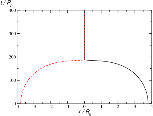
Figure 1: BH trajectories for an equal-mass head-on collision of two non-spinning holes initially at rest in $D=7$ dimensions. The collision takes place along the $x$ axis.

In order to check the consistency of our numerical formalism, we have also analyzed the constraint equations for this configuration. A snapshot of the Hamiltonian constraint (16) along the collision axis at evolution time $t=80~{}R_{h}$ is shown in Fig. 2. In this figure, the result obtained for the high resolution run has been amplified by a factor of four expected for second-order convergence. The overlap of the two curves demonstrates convergence at second order, compatible with the numerical scheme that employs second and fourth-order accurate discretization and interpolation techniques.

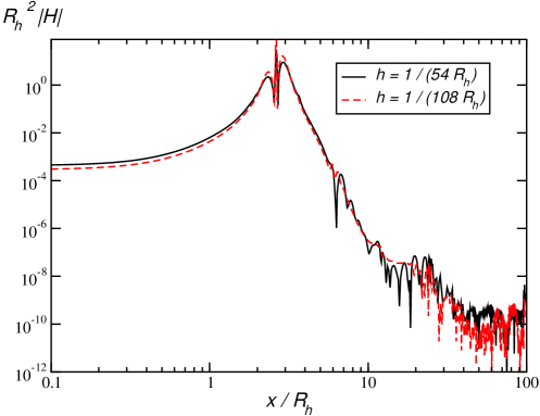
Figure 2: The Hamiltonian constraint along the collision axis obtained for a BH head-on collision starting from rest using resolution parameters $\Delta x=R_{h}/52$ (solid, black curve) and $\Delta x=R_{h}/104$ (dashed, red curve). The latter has been amplified by a factor of four corresponding to second-order convergence.

We have performed the same analysis for the Hamiltonian and momentum constraints at several points in time and observe the same second-order convergence of both constraints throughout infall and merger. Note that only one BH is present on the computational domain (at about $x=2.5$ in the figure) because of the octant symmetry. The other BH is represented in this simulation through the symmetric boundary conditions imposed at $x=0$.

6 Conclusions

In the presence of rotational symmetry, the Einstein equations simplify considerably and the generation of numerical solutions to these equations can be implemented with significant improvements in computational cost and the required amount of computer memory. The Cartoon method proposed in [47] was the first technique designed with the particular goal of efficiently modeling axisymmetric spacetimes in 3+1 numerical relativity. A modification, often dubbed the modified Cartoon method [1] used relations between tensor components in place of spatial interpolation operations, which not only eliminates the need of introducing a few extra grid points in the symmetry directions, but also allows for a particularly convenient generalization to an arbitrary number of spacetime dimensions and number of rotational symmetries [12, 48, 49].

In this work, we have presented in detail the complete set of equations as obtained for the BSSN formulation of the Einstein equations in $D$ spacetime dimensions with $SO(D-d)$ isometry where $d\in\{1,\,2,\,\ldots,\,D-2\}$. Furthermore, we explicitly demonstrate the presence of extra terms for the case $d=D-2$, where the symmetry condition allows for a wider class of components of tensor densities to remain non-zero. Finally, we have compiled a list of terms involving division by the quasi-radial coordinate (the $z$ direction in our case) and illustrate how all irregularities at the origin $z=0$ can be cured through equivalence with manifestly regular expressions. Even though we used the BSSN formulation for our discussion, the recipes detailed here can be applied straightforwardly to other popular formulations of the Einstein equations such as the generalized harmonic gauge [69, 1] or the conformal $Z4$ [70, 71] systems.

As an example, we have presented results from a head-on collision from rest of two equal-mass, non-spinning BHs in $D=7$ spacetime dimensions. Following a rather slow acceleration phase, due to the rapid diminishing of the gravitational force with distance, the two BHs merge and we observe second-order convergence of the constraints. This confirms in yet another type of application the remarkable robustness observed for the modified Cartoon method in applications to spinning BHs[12] or high-energy collisions in $D=5$ [42]. This seemingly superior robustness as compared with the method of reduction by isometry developed in [45] is, at present, empirical but merits further investigation at the analytic level.

Appendix A Cartesian components in $SO(D-d)$ symmetry

We present here the list of all modified cartoon expressions for the case of $SO(D-d)$ symmetry with $d<D-2$. The index range for early Latin indices is $a,\,b,\,\ldots=d+1,\,\ldots,\,D-1$ and for middle Latin indices $i,\,j,\,\ldots=1,\,\ldots\,d$. Furthermore, an index $z$ denotes the coordinate $z$ while the index $w$ only appears in the tensor component $T_{ww}$ which represents the additional function that needs to be evolved numerically in addition to the $T_{ij}$. For example, the spacetime metric is fully described by the components $g_{\alpha\beta}$, $\alpha,\,\beta=0,\,1,\,\ldots\,d$, plus one additional field $g_{ww}$. For arbitrary scalar, vector and tensor densities $\Psi$, $V^{{\scriptscriptstyle{A}}}$ and $T_{{\scriptscriptstyle{A}}{\scriptscriptstyle{B}}}$, the expressions are

$$0 = \partial_{a}\Psi=\partial_{i}\partial_{a}\Psi\,,$$ (59)

$$\partial_{a}\partial_{b}\Psi = \delta_{ab}\frac{\partial_{z}\Psi}{z}\,,$$ (60)

$$0 = V^{a}=\partial_{i}V^{a}=\partial_{a}V^{i}=\partial_{a}\partial_{b}V^{c}\,,$$ (61)

$$\partial_{a}V^{b} = \delta_{a}{}^{b}\frac{V^{z}}{z}\,,$$ (62)

$$\partial_{i}\partial_{a}V^{b} = \delta^{b}{}_{a}\left(\frac{\partial_{i}V^{z}}{z}-\delta_{iz}\frac{V^{z}}{z^{2}}\right)\,,$$ (63)

$$\partial_{a}\partial_{b}V^{i} = \delta_{ab}\left(\frac{\partial_{z}V^{i}}{z}-\delta^{i}{}_{z}\frac{V^{z}}{z^{2}}\right)\,,$$ (64)

$$0 = T_{ia}=\partial_{a}T_{bc}=\partial_{i}\partial_{a}T_{bc}=\partial_{a}\partial_{b}T_{ic}=\partial_{a}T_{ij}=\partial_{i}\partial_{a}T_{jk}\,,$$ (65)

$$T_{ab} = \delta_{ab}T_{ww}\,,$$ (66)

$$\partial_{a}\partial_{b}T_{cd} = (\delta_{ac}\delta_{bd}+\delta_{ad}\delta_{bc})\frac{T_{zz}-T_{ww}}{z^{2}}+\delta_{ab}\delta_{cd}\frac{\partial_{z}T_{ww}}{z}\,,$$ (67)

$$\partial_{a}T_{ib} = \delta_{ab}\frac{T_{iz}-\delta_{iz}T_{ww}}{z}\,,$$ (68)

$$\partial_{i}\partial_{a}T_{jb} = \delta_{ab}\left(\frac{\partial_{i}T_{jz}-\delta_{jz}\partial_{i}T_{ww}}{z}-\delta_{iz}\frac{T_{jz}-\delta_{jz}T_{ww}}{z^{2}}\right)\,,$$ (69)

$$\partial_{a}\partial_{b}T_{ij} = \delta_{ab}\left(\frac{\partial_{z}T_{ij}}{z}-\frac{\delta_{iz}T_{jz}+\delta_{jz}T_{iz}-2\delta_{iz}\delta_{jz}T_{ww}}{z^{2}}\right)\,.$$ (70)

Appendix B Regularization at $z=0$ for $d<D-2$

The presence of $z$ in the denominator of several terms in the system of Eqs. (31)-(51) merely arises from the quasi-radial nature of the coordinate $z$ and can be handled straightforwardly in analogy to the treatment of the origin in spherical or axisymmetry.

We will present the regularized terms needed in the generic $SO(D-d)$ symmetry; however, it should be noted that terms involving the inverse metric become much more complicated for a large $d$, and so we will also explicitly show these terms for the most common case, $d=3$.

We first require that all components expressed in a fully Cartesian set of coordinates are regular. A well known consequence of this assumption is that tensor density components containing an odd (even) number of radial, i.e. $z$, indices contain only odd (even) powers of $z$ in a series expansion around $z=0$. The same holds for quantities derived from tensors and densities such as the BSSN variable $\tilde{\Upgamma}^{i}$.

Next, we consider the inverse metric which we obtain through inversion of the matrix equation (30). By constructing the cofactor matrix and dividing by the determinant, we obtain, for $d=3$

$$\begin{array}[]{lll}\tilde{\gamma}^{xx}=\tilde{\gamma}_{ww}^{n}\frac{\tilde{\gamma}_{yy}\tilde{\gamma}_{zz}-\tilde{\gamma}_{yz}^{2}}{\det\tilde{\gamma}_{{\scriptscriptstyle{I}}{\scriptscriptstyle{J}}}}\,,{}&\tilde{\gamma}^{xy}=\tilde{\gamma}_{ww}^{n}\frac{\tilde{\gamma}_{yz}\tilde{\gamma}_{xz}-\tilde{\gamma}_{xy}\tilde{\gamma}_{zz}}{\det\tilde{\gamma}_{{\scriptscriptstyle{I}}{\scriptscriptstyle{J}}}}\,,{}&\tilde{\gamma}^{xz}=\tilde{\gamma}_{ww}^{n}\frac{\tilde{\gamma}_{xy}\tilde{\gamma}_{yz}-\tilde{\gamma}_{xz}\tilde{\gamma}_{yy}}{\det\tilde{\gamma}_{{\scriptscriptstyle{I}}{\scriptscriptstyle{J}}}}\,,\\[10.0pt] \cdots&\tilde{\gamma}^{yy}=\tilde{\gamma}_{ww}^{n}\frac{\tilde{\gamma}_{xx}\tilde{\gamma}_{zz}-\tilde{\gamma}_{xz}^{2}}{\det\tilde{\gamma}_{{\scriptscriptstyle{I}}{\scriptscriptstyle{J}}}}\,,&\tilde{\gamma}^{yz}=\tilde{\gamma}_{ww}^{n}\frac{\tilde{\gamma}_{xy}\tilde{\gamma}_{xz}-\tilde{\gamma}_{xx}\tilde{\gamma}_{yz}}{\det\tilde{\gamma}_{{\scriptscriptstyle{I}}{\scriptscriptstyle{J}}}}\,,\\[10.0pt] \cdots&\cdots&\tilde{\gamma}^{zz}=\tilde{\gamma}_{ww}^{n}\frac{\tilde{\gamma}_{xx}\tilde{\gamma}_{yy}-\tilde{\gamma}_{xy}^{2}}{\det\tilde{\gamma}_{{\scriptscriptstyle{I}}{\scriptscriptstyle{J}}}}\,.\end{array}$$ (71)

Next, we recall that the BSSN metric has unit determinant, so that

$$1=\det\tilde{\gamma}_{{\scriptscriptstyle{I}}{\scriptscriptstyle{J}}} = \tilde{\gamma}_{ww}^{n}(\tilde{\gamma}_{xx}\tilde{\gamma}_{yy}\tilde{\gamma}_{zz}+2\tilde{\gamma}_{xy}\tilde{\gamma}_{xz}\tilde{\gamma}_{yz}-\tilde{\gamma}_{xx}\tilde{\gamma}_{yz}^{2}-\tilde{\gamma}_{yy}\tilde{\gamma}_{xz}^{2}-\tilde{\gamma}_{zz}\tilde{\gamma}_{xy}^{2})$$ (72)

$$\overset{*}{=} \tilde{\gamma}_{ww}^{n}\tilde{\gamma}_{zz}(\tilde{\gamma}_{xx}\tilde{\gamma}_{yy}-\tilde{\gamma}_{xy}^{2})\,,$$

where we introduced the symbol “$\,\overset{*}{=}\,$” to denote equality in the limit $z\rightarrow 0$. The components for the inverse BSSN metric in Eq. (71) simplify accordingly.

For a general $d$ we know that the matrix takes the form given in Eq (30). Then, denoting the cofactor matrix for a given element of $\tilde{\gamma}_{{\scriptscriptstyle{I}}{\scriptscriptstyle{J}}}$ as $C_{{\scriptscriptstyle{I}}{\scriptscriptstyle{J}}}$, the inverse BSSN metric components are (note that the metric is symmetric, so that $C_{{\scriptscriptstyle{I}}{\scriptscriptstyle{J}}}=C_{{\scriptscriptstyle{J}}{\scriptscriptstyle{I}}}$)

$$\begin{array}[]{cccc}\tilde{\gamma}^{x^{1}x^{1}}=\frac{C_{x^{1}x^{1}}}{\det{\tilde{\gamma}_{{\scriptscriptstyle{I}}{\scriptscriptstyle{J}}}}}\,,{}&\cdots\,,{}&\tilde{\gamma}^{x^{1}x^{d-1}}=\frac{C_{x^{1}x^{d-1}}}{\det{\tilde{\gamma}_{{\scriptscriptstyle{I}}{\scriptscriptstyle{J}}}}}\,,{}&\tilde{\gamma}^{x^{1}z}=\frac{C_{x^{1}z}}{\det{\tilde{\gamma}_{{\scriptscriptstyle{I}}{\scriptscriptstyle{J}}}}}\,,\\[10.0pt] \vdots&\ddots&\vdots&\vdots\\[10.0pt] \vdots&\cdots&\tilde{\gamma}^{x^{d-1}x^{d-1}}=\frac{C_{x^{d-1}x^{d-1}}}{\det{\tilde{\gamma}_{{\scriptscriptstyle{I}}{\scriptscriptstyle{J}}}}},&\tilde{\gamma}^{x^{d-1}z}=\frac{C_{x^{d-1}z}}{\det{\tilde{\gamma}_{{\scriptscriptstyle{I}}{\scriptscriptstyle{J}}}}}\\[10.0pt] \cdots&\cdots&\cdots&\tilde{\gamma}^{zz}=\frac{C_{zz}}{\det{\tilde{\gamma}_{{\scriptscriptstyle{I}}{\scriptscriptstyle{J}}}}}\,.\end{array}$$ (73)

Again, in the BSSN case $\det\tilde{\gamma}_{{\scriptscriptstyle{I}}{\scriptscriptstyle{J}}}=1$, and the inverse metric element is simply the cofactor of that element. For simplicity, we will use indices $\hat{i}$ in place of $x^{\hat{i}}$ in the remainder of this section, so that, for example $C_{12}\equiv C_{x^{1}x^{2}}$, $C_{1z}\equiv C_{x^{1}z}$ etc. When used without a caret, the lower case Latin indices $i,\,j,\,\ldots$ also include the $z$ component.

If we denote the upper-left quadrant of the matrix in Eq (30) as the matrix $M_{ij}$, then we can write the cofactor of an element in this upper-left quadrant as

$$C_{ij}=(-1)^{i+j}\tilde{\gamma}_{ww}^{n}\det(M_{kl\{k\neq j,l\neq i\}})\,.$$ (74)

Here, the notation $\det(M_{kl\{k\neq j,l\neq i\}})$ denotes the determinant of the matrix obtained by crossing out the $j^{\rm th}$ row and $i^{\rm th}$ column. Likewise, we may add further inequalities inside the braces to denote matrices obtained by crossing out more than one row and column.

The next regularity condition we require our spacetime to satisfy is the absence of a conical singularity at $z=0$. In polar coordinates $(\rho,\varphi)$ constructed as in Sec. 2.2, this condition can be expressed as $\tilde{\gamma}_{\varphi\varphi}=\rho^{2}\tilde{\gamma}_{\rho\rho}$ which translates into the conditions

$$\tilde{\gamma}_{zz}-\tilde{\gamma}_{ww}\overset{*}{=}\mathcal{O}(z^{2})\,,~{}~{}~{}~{}~{}~{}~{}\tilde{\gamma}^{zz}-\tilde{\gamma}^{ww}\overset{*}{=}\mathcal{O}(z^{2})\,,~{}~{}~{}$$ (75)

in Cartesian coordinates. By taking the time derivative of these relations and combining these with Eqs. (34), (35), we obtain an analogous relation for the traceless extrinsic curvature,

$$\tilde{A}_{zz}-\tilde{A}_{ww}\overset{*}{=}\mathcal{O}(z^{2})\,.$$ (76)

We thus arrive at the following list of regularized terms valid in the limit $z\rightarrow 0$.

• By expanding $\beta^{z}=b_{1}z+b_{3}z^{3}+\ldots$, and likewise for $\tilde{\Gamma}^{z}$ and $\partial_{z}\tilde{\gamma}_{ww}$, we obtain

  $$\frac{\beta^{z}}{z}\overset{*}{=}\partial_{z}\beta_{z}\,,~{}~{}~{}~{}~{}~{}\frac{\tilde{\Gamma}^{z}}{z}\overset{*}{=}\partial_{z}\tilde{\Gamma}^{z}\,,~{}~{}~{}~{}~{}~{}\frac{\partial_{z}\tilde{\gamma}_{ww}}{z}\overset{*}{=}\partial_{z}\partial_{z}\tilde{\gamma}_{ww}\,,$$ (77)

  and likewise for $\alpha$ or $\chi$ in place of $\tilde{\gamma}_{ww}$ in the last expression.

• We express the inverse metric components through their cofactors, given for arbitrary $d$ by Eq. (74), and then apply the same trading of divisions by $z$ for derivatives as done for $\beta^{z}/z$, to obtain

  $$\frac{\delta^{i}{}_{z}-\tilde{\gamma}^{zi}\tilde{\gamma}_{ww}}{z}\overset{*}{=}\left\{\begin{array}[]{ll}\displaystyle\sum_{\hat{m}=1}^{d-1}(-1)^{\hat{m}+\hat{i}}\partial_{z}(\tilde{\gamma}_{{\hat{m}}z})\tilde{\gamma}_{ww}^{n+1}\det(M_{jl\{j\neq z,j\neq\hat{m},l\neq i,l\neq z\}}){}{}&\text{if }i=\hat{i}\\[20.0pt] 0&\text{if }i=z\end{array}\right.\,.$$ (78)

  Here, as well in items (5) and (9) below, we formally set $\det(M_{jl\{j\neq z,j\neq\hat{m},l\neq i,l\neq z\}})=1$ for the case $d=2$ where no entries would be left in the matrix after crossing out two rows and columns. For $d=1$, the case $i=\hat{i}$ does not arise which obviates the need to evaluate the determinant. For the case $d=3$, the expression (78) becomes

  $$\frac{\delta^{i}{}_{z}-\tilde{\gamma}^{zi}\tilde{\gamma}_{ww}}{z}\overset{*}{=}\left\{\begin{array}[]{ll}\tilde{\gamma}_{ww}^{n+1}(\tilde{\gamma}_{yy}\partial_{z}\tilde{\gamma}_{xz}-\tilde{\gamma}_{xy}\partial_{z}\tilde{\gamma}_{yz}){}{}{}{}&\text{if }i=x\\[10.0pt] \tilde{\gamma}_{ww}^{n+1}(\tilde{\gamma}_{xx}\partial_{z}\tilde{\gamma}_{yz}-\tilde{\gamma}_{xy}\partial_{z}\tilde{\gamma}_{xz}){}{}{}{}&\text{if }i=y\\[10.0pt] 0&\text{if }i=z\end{array}\right.\,.$$ (79)

• Expanding $\beta^{\hat{i}}=b_{0}+b_{2}z^{2}+\ldots$ and $\beta^{z}=b_{1}z+b_{3}z^{3}+\ldots$ , we trade two divisions by $z$ for a second derivative and obtain

  $$\frac{\partial_{z}\beta^{i}}{z}-\delta^{i}{}_{z}\frac{\beta^{z}}{z^{2}}=\left\{\begin{array}[]{ll}\partial_{z}\partial_{z}\beta^{\hat{i}}{}{}{}&\text{if }i=\hat{i}\\[10.0pt] 0&\text{if }i=z\end{array}\right.\,.$$ (80)

• We rewrite the term

  $$\frac{\tilde{\gamma}^{im}\partial_{m}\beta^{z}}{z}-\tilde{\gamma}^{iz}\frac{\beta^{z}}{z^{2}}=\tilde{\gamma}^{im}\left(\frac{\partial_{m}\beta^{z}}{z}-\delta^{z}{}_{m}\frac{\beta^{z}}{z^{2}}\right)\,,$$ (81)

  and expand $\beta^{z}=b_{1}z+b_{3}z^{3}+\ldots$ which leads to

  $$\frac{\partial_{m}\beta^{z}}{z}-\delta^{z}{}_{m}\frac{\beta^{z}}{z^{2}}=\left\{\begin{array}[]{ll}\partial_{\hat{m}}\partial_{z}\beta^{z}{}{}{}&\text{if }m=\hat{m}\\[10.0pt] 0&\text{if }m=z\end{array}\right.\,.$$ (82)

• Similarly to Eq. (78), we find for general $d$ that

  $$\frac{\tilde{\gamma}^{zm}}{z}\partial_{m}\alpha = \sum_{\hat{m}=1}^{d-1}\sum_{\hat{i}=1}^{d-1}(-1)^{\hat{m}+\hat{i}-1}\partial_{z}(\tilde{\gamma}_{{\hat{m}}z})\tilde{\gamma}_{ww}^{n}\det(M_{jl\{j\neq z,j\neq\hat{m},l\neq\hat{i},l\neq z\}})\partial_{\hat{i}}\alpha$$ (83)

  $$+\tilde{\gamma}^{zz}\partial_{z}\partial_{z}\alpha\,,$$

  where again we formally set $\det(M_{jl\{j\neq z,j\neq\hat{m},l\neq i,l\neq z\}})=1$ for the case $d=2$; cf. item (2) above. For $d=3$, we obtain

  $$\frac{\tilde{\gamma}^{zm}}{z}\partial_{m}\alpha = \tilde{\gamma}_{ww}^{n}\left[\left(\tilde{\gamma}_{xy}\partial_{z}\tilde{\gamma}_{yz}-\tilde{\gamma}_{yy}\partial_{z}\tilde{\gamma}_{xz}\right)\partial_{x}\alpha+\left(\tilde{\gamma}_{xy}\partial_{z}\tilde{\gamma}_{xz}-\tilde{\gamma}_{xx}\partial_{z}\tilde{\gamma}_{yz}\right)\partial_{y}\alpha\right]$$ (84)

  $$+\tilde{\gamma}^{zz}\partial_{z}\partial_{z}\alpha\,,$$

  and likewise for $\chi$ in place of $\alpha$.

• Using $\tilde{A}_{zz}-\tilde{A}_{ww}=\mathcal{O}(z^{2})$, we obtain

  $$\frac{\tilde{A}_{iz}-\delta_{iz}\tilde{A}_{ww}}{z}=\left\{\begin{array}[]{ll}\partial_{z}\tilde{A}_{\hat{i}z}{}{}{}{}{}&\text{if }i=\hat{i}\\[10.0pt] 0&\text{if }i=z\end{array}\right.\,.$$ (85)

• Using $\tilde{\gamma}_{zz}-\tilde{\gamma}_{ww}=\mathcal{O}(z^{2})$ and trading a division by $z$ for a $z$ derivative, we find

  $$-\frac{1}{2}\frac{\partial_{z}\tilde{\gamma}_{ij}}{z}+\frac{\delta_{z(i}\tilde{\gamma}_{j)z}-\delta_{iz}\delta_{jz}\tilde{\gamma}_{ww}}{z^{2}}=\left\{\begin{array}[]{ll}-\frac{1}{2}\partial_{z}\partial_{z}\tilde{\gamma}_{\hat{i}\hat{j}}{}{}{}{}{}&\text{if }(i,j)=(\hat{i},\hat{j})\\[10.0pt] 0&\text{if }(i,j)=(\hat{i},z)\text{ or }(z,\hat{j})\\[10.0pt] -\frac{1}{2}\partial_{z}\partial_{z}\tilde{\gamma}_{ww}&\text{if }(i,j)=(z,z)\end{array}\right.\,.$$ (86)

• Using $\tilde{\gamma}^{ww}\tilde{\gamma}_{zz}-1=\tilde{\gamma}^{ww}(\tilde{\gamma}_{zz}-\gamma_{ww})=\tilde{\gamma}^{ww}\mathcal{O}(z^{2})$ and $\tilde{\gamma}_{z\hat{i}}/z=\partial_{z}\tilde{\gamma}_{z\hat{i}}$, we can rewrite

  $$\frac{\tilde{\gamma}^{ww}\tilde{\gamma}_{z(j}-\delta_{z(j}}{z}\partial_{i)}\tilde{\gamma}_{ww}=\left\{\begin{array}[]{ll}\tilde{\gamma}^{ww}\partial_{z}\tilde{\gamma}_{z(\hat{j}}\partial_{\hat{i})}\tilde{\gamma}_{ww}{}{}{}{}{}&\text{if }(i,j)=(\hat{i},\hat{j})\\[10.0pt] 0&\text{if }(i,j)=(\hat{i},z)\text{ or }(z,\hat{j})\\[10.0pt] 0&\text{if }(i,j)=(z,z)\end{array}\right.\,.$$ (87)

• The term $(\tilde{\gamma}^{zz}\tilde{\gamma}_{ww}-1)/z^{2}$ requires slightly more work and we describe its derivation here in a little more detail. We first rewrite this term in the form

  $$\frac{\tilde{\gamma}^{zz}\tilde{\gamma}_{ww}-1}{z^{2}}=-\tilde{\gamma}^{zz}\frac{\frac{1}{\tilde{\gamma}^{zz}}-\tilde{\gamma}_{ww}}{z^{2}}\,,$$ (88)

  and express the inverse metric component $\tilde{\gamma}^{zz}$ in terms of the corresponding cofactor matrix component and the determinant as

  $$\frac{1}{{\tilde{\gamma}^{zz}}}=\frac{\det{\tilde{\gamma}_{{\scriptscriptstyle{I}}{\scriptscriptstyle{J}}}}}{C_{zz}}=\frac{\tilde{\gamma}_{zz}C_{zz}}{C_{zz}}+\frac{\sum_{\hat{i}=1}^{d-1}\tilde{\gamma}_{z{\hat{i}}}C_{zx_{\hat{i}}}}{C_{zz}}.$$ (89)

  Note that these expressions are all valid for arbitrary values of $z$ and we are not yet using the BSSN condition $\det{\tilde{\gamma}}_{{\scriptscriptstyle{I}}{\scriptscriptstyle{J}}}=1$. We can now plug this relation into Eq. (88). We then trade divisions by $z$ for derivatives with respect to $z$, bearing in mind that $\tilde{\gamma}_{zz}=\tilde{\gamma}_{ww}+\mathcal{O}(z^{2})$ and find

  $$\frac{\tilde{\gamma}^{zz}\tilde{\gamma}_{ww}-1}{z^{2}}\overset{*}{=}\frac{\tilde{\gamma}^{zz}}{2}\left(\partial_{z}\partial_{z}\tilde{\gamma}_{ww}-\partial_{z}\partial_{z}\tilde{\gamma}_{zz}\right)$$ (90)

  $$~{}~{}~{}~{}~{}~{}+\tilde{\gamma}^{zz}\sum_{\hat{i}=1}^{d-1}\sum_{\hat{j}=1}^{d-1}(-1)^{\hat{i}+\hat{j}}\,\tilde{\gamma}_{ww}^{n}\frac{\partial_{z}\tilde{\gamma}_{z\hat{i}}\,\partial_{z}\tilde{\gamma}_{\hat{j}z}}{C_{zz}}\det(M_{kl\{k\neq z,k\neq\hat{j},l\neq\hat{i},l\neq z\}})\,.$$

  Again, we formally set $\det(M_{jl\{j\neq z,j\neq\hat{m},l\neq i,l\neq z\}})=1$ for the case $d=2$; cf. item (2) above. Finally we use $1=\det\tilde{\gamma}_{{\scriptscriptstyle{I}}{\scriptscriptstyle{J}}}\Rightarrow C_{zz}=\tilde{\gamma}^{zz}$ to obtain

  $$\frac{\tilde{\gamma}^{zz}\tilde{\gamma}_{ww}-1}{z^{2}} \overset{*}{=} \frac{\tilde{\gamma}^{zz}}{2}\left(\partial_{z}\partial_{z}\tilde{\gamma}_{ww}-\partial_{z}\partial_{z}\tilde{\gamma}_{zz}\right)$$

  $$+\sum_{\hat{i}=1}^{d-1}\sum_{\hat{j}=1}^{d-1}(-1)^{\hat{i}+\hat{j}}\,\tilde{\gamma}_{ww}^{n}(\partial_{z}\tilde{\gamma}_{z{\hat{i}}})\,\partial_{z}\tilde{\gamma}_{z\hat{j}}\det(M_{kl\,\{k\neq z,k\neq\hat{j},l\neq\hat{i},l\neq z\}})\,.$$

  For the case $d=3$ this reduces to:

  $$\frac{\tilde{\gamma}^{zz}\tilde{\gamma}_{ww}-1}{z^{2}} \overset{*}{=} \frac{\tilde{\gamma}^{zz}}{2}\partial_{z}\partial_{z}(\tilde{\gamma}_{ww}-\tilde{\gamma}_{zz})-\tilde{\gamma}_{ww}^{n}\left[2\tilde{\gamma}_{xy}(\partial_{z}\tilde{\gamma}_{xz})\partial_{z}\tilde{\gamma}_{yz}-\tilde{\gamma}_{xx}(\partial_{z}\tilde{\gamma}_{yz})^{2}\right.$$ (92)

  $$\left.-\tilde{\gamma}_{yy}(\partial_{z}\tilde{\gamma}_{xz})^{2}\right]\,.$$

Appendix C Cartesian components in $SO(2)$ symmetry

The general case of $SO(2)$ symmetry requires some modifications to the expressions given in A. Here we list these necessary changes. Recall that lower case Latin indices with a caret range from $1,...,D-3$, since $d=D-2$.

The expressions for scalars (59) and (60) remain unchanged. For vectors, Eq. (61) no longer holds in $SO(2)$ symmetry and is replaced by

$$\partial_{w}V^{i} = -\delta^{i}{}_{z}\frac{V^{w}}{z}\,,$$ (93)

$$\partial_{i}\partial_{w}V^{j} = \delta^{j}{}_{z}\left(-\frac{\partial_{i}V^{w}}{z}+\delta^{z}{}_{i}\frac{V^{w}}{z^{2}}\right)\,,$$ (94)

$$\partial_{w}\partial_{w}V^{w} = \frac{\partial_{z}V^{w}}{z}-\frac{V^{w}}{z^{2}}\,.$$ (95)

For rank two tensors, Eq. (65) no longer holds. Instead, we have

$$\partial_{w}T_{\hat{i}\hat{j}} = 0\,,$$ (96)

$$\partial_{w}T_{iz} = -\frac{1}{z}T_{iw}-\delta_{zi}\frac{T_{zw}}{z}\,,$$ (97)

$$\partial_{w}T_{ww} = 2\frac{T_{zw}}{z}\,,$$ (98)

$$\partial_{i}\partial_{w}T_{\hat{i}\hat{j}} = 0\,,$$ (99)

$$\partial_{i}\partial_{w}T_{jz} = -\frac{\partial_{i}T_{jw}+\delta_{zj}\partial_{i}T_{wz}}{z}+\delta_{iz}\frac{T_{jw}+\delta_{zj}T_{zw}}{z^{2}}\,,$$ (100)

$$\partial_{i}\partial_{w}T_{ww} = 2\frac{\partial_{i}T_{zw}}{z}-2\delta_{iz}\frac{T_{zw}}{z^{2}}\,,$$ (101)

$$\partial_{w}\partial_{w}T_{iw} = \frac{\partial_{z}T_{iw}}{z}-\frac{T_{iw}+3\delta_{iz}T_{zw}}{z^{2}}\,.$$ (102)

As for the case of $SO(D-d)$ symmetry the above expressions need to be regularized at $z=0$. For Eqs. (93-95), we note that $SO(2)$ symmetry implies that vector components $V^{w}$ are odd functions of $z$ on the $w=0$ hyperplane. Therefore, the regularization of vector components follows the procedure in Eqs. (77) and (82).

For the regularization of Eqs. (96-102), note that components of type $T_{\hat{i}w}$ behave like vector components, that is they are odd functions of $z$. The component $T_{zw}$, on the other hand, has to vanish at $z=0$ and must be an even function of $z$. The latter can be seen by contracting $T_{\mu\nu}$ with two vectors pointing in the $w$ and $z$ direction respectively. The result must be a scalar which satisfies the symmetry and is therefore even. Together with the fact that $z$ and $w$ components of vectors are odd this then implies that $T_{zw}$ is even.

Combining these relations with those previously discussed in B, we obtain the following regularized terms specific to the case of $SO(2)$ symmetry.

$$\frac{V^{w}}{z} \overset{*}{=} \partial_{z}V^{w}\,,$$ (103)

$$-\frac{\partial_{i}V^{w}}{z}+\delta^{z}{}_{i}\frac{V^{w}}{z^{2}} \overset{*}{=} \left\{\begin{array}[]{ll}-\partial_{i}\partial_{z}V^{w}{}{}{}{}{}&\text{if }i=\hat{i}\\[10.0pt] 0&\text{if }i=z\end{array}\right.\,,$$ (106)

$$-\frac{T_{iw}}{z}-\delta_{zi}\frac{T_{zw}}{z} \overset{*}{=} \left\{\begin{array}[]{ll}-\partial_{z}T_{iw}{}{}{}{}{}&\text{if }i=\hat{i}\\[10.0pt] 0&\text{if }i=z\end{array}\right.\,,$$ (109)

$$-\frac{\partial_{i}T_{jw}+\delta_{jz}\partial_{i}T_{wz}}{z}+\delta_{iz}\frac{T_{jw}+\delta_{zj}T_{zw}}{z^{2}} \overset{*}{=} \left\{\begin{array}[]{ll}-\partial_{i}\partial_{z}T_{jw}{}{}{}{}{}&\text{if }(i,j)=(\hat{i},\hat{j})\\[10.0pt] 0&\text{if }(i,j)=(z,\hat{j})\text{ or }(\hat{i},z)\\[10.0pt] -\partial_{z}\partial_{z}T_{wz}&\text{if }(i,j)=(z,z)\end{array}\right.\,,$$ (113)

$$2\frac{\partial_{i}T_{zw}}{z}-2\delta_{iz}\frac{T_{zw}}{z^{2}} \overset{*}{=} \left\{\begin{array}[]{ll}0&\text{if }i=\hat{i}\\[10.0pt] \partial_{z}\partial_{z}T_{zw}{}{}{}{}{}&\text{if }i=z\end{array}\right.\,,$$ (117)

$$\frac{\partial_{z}T_{iw}}{z}-\frac{T_{iw}+3\delta_{iz}T_{zw}}{z^{2}} \overset{*}{=} \left\{\begin{array}[]{ll}0&\text{if }i=\hat{i}\\[10.0pt] -\partial_{z}\partial_{z}T_{zw}{}{}{}{}{}&\text{if }i=z\end{array}\right.\,.$$ (120)

Finally, we list for completeness the regularization of Eqs. (60), (63), (64), (67), (68) and (69) expressed here in terms of generic vector and tensor fields rather than the BSSN variables,

$$\frac{\partial_{z}\psi}{z} \overset{*}{=} \partial_{z}\partial_{z}\psi\,,$$ (121)

$$\frac{V^{z}}{z} \overset{*}{=} \partial_{z}V^{z}\,,$$ (122)

$$\frac{\partial_{i}V^{z}}{z}-\delta^{z}{}_{i}\frac{V^{z}}{z^{2}} \overset{*}{=} \left\{\begin{array}[]{ll}\partial_{i}\partial_{z}V^{z}{}{}{}{}{}&\text{if }i=\hat{i}\\[10.0pt] 0&\text{if }i=z\end{array}\right.\,,$$ (125)

$$\frac{\partial_{z}V^{i}}{z}-\delta^{i}{}_{z}\frac{V^{z}}{z^{2}} \overset{*}{=} \left\{\begin{array}[]{ll}\partial_{z}\partial_{z}V^{i}{}{}{}{}{}&\text{if }i=\hat{i}\\[10.0pt] 0&\text{if }i=z\end{array}\right.\,,$$ (128)

$$\frac{T_{zz}-T_{ww}}{z^{2}} \overset{*}{=} \frac{1}{2}\partial_{z}\partial_{z}(T_{zz}-T_{ww})\,,$$ (129)

$$\frac{\partial_{z}T_{ww}}{z} \overset{*}{=} \partial_{z}\partial_{z}T_{ww}\,,$$ (130)

$$\frac{T_{iz}-\delta_{iz}T_{ww}}{z} \overset{*}{=} \left\{\begin{array}[]{ll}\partial_{z}T_{iz}{}{}{}{}{}&\text{if }i=\hat{i}\\[10.0pt] 0&\text{if }i=z\end{array}\right.\,,$$ (133)

$$\frac{\partial_{i}T_{jz}-\delta_{jz}\partial_{i}T_{ww}}{z}-\delta_{iz}\frac{T_{jz}-\delta_{jz}T_{ww}}{z^{2}} \overset{*}{=} \left\{\begin{array}[]{ll}\partial_{i}\partial_{z}T_{jz}{}{}{}{}{}&\text{if }(i,j)=(\hat{i},\hat{j})\\[10.0pt] 0&\text{if }(i,j)=(\hat{i},z)\text{ or }(z,\hat{j})\\[10.0pt] \frac{\partial_{z}\partial_{z}(T_{zz}-T_{ww})}{2}&\text{if }(i,j)=(z,z)\end{array}\right.\,,$$ (137)

$$\frac{\partial_{z}T_{ij}}{z}-\frac{\delta_{iz}T_{jz}+\delta_{jz}T_{iz}-2\delta_{iz}\delta_{jz}T_{ww}}{z^{2}} \overset{*}{=} \left\{\begin{array}[]{ll}\partial_{z}\partial_{z}T_{ij}{}{}{}{}{}&\text{if }(i,j)=(\hat{i},\hat{j})\\[10.0pt] 0&\text{if }(i,j)=(\hat{i},z)\text{ or }(z,\hat{j})\\[10.0pt] \partial_{z}\partial_{z}T_{ww}&\text{if }(i,j)=(z,z)\end{array}\right.\,.$$ (142)

References

- [1] F. Pretorius, Class. Quantum Grav. 22 (2005) 425, gr-qc/0407110.
- [2] B. â. Abbott et al., Phys. Rev. Lett. 116 (2016) 061102, arXiv:1602.03837 [gr-qc].
- [3] J. S. Read et al., Phys. Rev. D 88 (2013) 044042, arXiv:1306.4065 [gr-qc].
- [4] I. Hinder et al., Class. Quant. Grav. 31 (2014) 025012, arXiv:1307.5307 [gr-qc].
- [5] F. Pretorius, Phys. Rev. Lett. 95 (2005) 121101, gr-qc/0507014.
- [6] J. G. Baker, J. Centrella, D.-I. Choi, M. Koppitz and J. van Meter, Phys. Rev. Lett. 96 (2006) 111102, gr-qc/0511103.
- [7] M. Campanelli, C. O. Lousto, P. Marronetti and Y. Zlochower, Phys. Rev. Lett. 96 (2006) 111101, gr-qc/0511048.
- [8] V. Cardoso, L. Gualtieri, C. Herdeiro and U. Sperhake, Living Rev. Relativity 18 (2015) 1, arXiv:1409.0014 [gr-qc].
- [9] R. Emparan and H. S. Reall, Living Reviews in Relativity 11 (2008) http://www.livingreviews.org/lrr-2008-6.
- [10] R. C. Myers and M. J. Perry, Annals Phys. 172 (1986) 304.
- [11] M. Shibata and H. Yoshino, Phys. Rev. D 81 (2010) 021501, arXiv:0912.3606 [gr-qc].
- [12] M. Shibata and H. Yoshino, Phys. Rev. D 81 (2010) 104035, arXiv:1004.4970 [gr-qc].
- [13] R. Gregory and R. Laflamme, Phys. Rev. Lett. 70 (1993) 2837, hep-th/9301052.
- [14] L. Lehner and F. Pretorius (2011) arXiv:1106.5184 [gr-qc].
- [15] P. Figueras, M. Kunesch and S. Tunyasuvunakool, Phys. Rev. Lett. 116 (2016) 071102, arXiv:1512.04532 [hep-th].
- [16] J. E. Santos and B. Way, Phys. Rev. Lett. 114 (2015) 221101, arXiv:1503.00721 [hep-th].
- [17] H. Bantilan, F. Pretorius and S. S. Gubser, Phys. Rev. D 85 (2012) 084038, arXiv:1201.2132 [hep-th].
- [18] P. M. Chesler and L. G. Yaffe, JHEP 1407 (2014) 086, arXiv:1309.1439 [hep-th].
- [19] H. Bantilan and P. Romatschke, Phys. Rev. Lett. 114 (2015) 081601, arXiv:1410.4799 [hep-th].
- [20] S. S. Gubser and W. van der Schee, JHEP 01 (2015) 028, arXiv:1410.7408 [hep-th].
- [21] P. M. Chesler, Phys. Rev. Lett. 115 (2015) 241602, arXiv:1506.02209 [hep-th].
- [22] A. Buchel, M. P. Heller and R. C. Myers, Phys. Rev. Lett. 114 (2015) 251601, arXiv:1503.07114 [hep-th].
- [23] I. Antoniadis, Phys. Lett. B 246 (1990) 377.
- [24] I. Antoniadis, N. Arkani-Hamed, S. Dimopoulos and G. R. Dvali, Phys. Lett. B 436 (1998) 257, hep-ph/9804398.
- [25] N. Arkani-Hamed, S. Dimopoulos and G. R. Dvali, Phys. Lett. B 429 (1998) 263, hep-ph/9803315.
- [26] L. Randall and R. Sundrum, Phys. Rev. Lett. 83 (1999) 3370, hep-ph/9905221.
- [27] L. Randall and R. Sundrum, Phys. Rev. Lett. 83 (1999) 4690, hep-th/9906064.
- [28] T. Banks and W. Fischler (1999) hep-th/9906038.
- [29] S. Dimopoulos and G. Landsberg, Phys. Rev. Lett. 87 (2001) 161602, hep-th/0106295.
- [30] S. B. Giddings and S. Thomas, Phys. Rev. D 65 (2002) 056010, hep-ph/0106219.
- [31] U. Sperhake, V. Cardoso, F. Pretorius, E. Berti and J. A. González, Phys. Rev. Lett. 101 (2008) 161101, arXiv:0806.1738 [gr-qc].
- [32] M. Shibata, H. Okawa and T. Yamamoto, Phys. Rev. D 78 (2008) 101501(R), arXiv:0810.4735 [gr-qc].
- [33] M. W. Choptuik and F. Pretorius, Phys. Rev. Lett. 104 (2010) 111101, arXiv:0908.1780 [gr-qc].
- [34] U. Sperhake, V. Cardoso, F. Pretorius, E. Berti, T. Hinderer and N. Yunes, Phys. Rev. Lett. 103 (2009) 131102, arXiv:0907.1252 [gr-qc].
- [35] W. E. East and F. Pretorius, Phys. Rev. Lett. 110 (2013) 101101, arXiv:1210.0443 [gr-qc].
- [36] L. Rezzolla and K. Takami, Class. Quant. Grav. 30 (2013) 012001, arXiv:1209.6138 [gr-qc].
- [37] U. Sperhake, E. Berti, V. Cardoso and F. Pretorius, Phys. Rev. Lett. 111 (2013) 041101, arXiv:1211.6114 [gr-qc].
- [38] J. Healy, I. Ruchlin and C. O. Lousto (2015) arXiv:1506.06153 [gr-qc].
- [39] U. Sperhake, E. Berti, V. Cardoso and F. Pretorius (2015) arXiv:1511.08209 [gr-qc].
- [40] H. Witek, M. Zilhão, L. Gualtieri, V. Cardoso, C. Herdeiro, A. Nerozzi and U. Sperhake, Phys. Rev. D 82 (2010) 104014, arXiv:1006.3081 [gr-qc].
- [41] H. Witek, V. Cardoso, L. Gualtieri, C. Herdeiro, U. Sperhake and M. Zilhão, Phys. Rev. D 83 (2011) 044017, arXiv:1011.0742 [gr-qc].
- [42] H. Okawa, K.-i. Nakao and M. Shibata, Phys. Rev. D 83 (2011) 121501, arXiv:1105.3331 [gr-qc].
- [43] H. Witek, H. Okawa, V. Cardoso, L. Gualtieri, C. Herdeiro, M. Shibata, U. Sperhake and M. Zilhão, Phys. Rev. D 90 (2014) 084014, arXiv:1406.2703 [gr-qc].
- [44] R. Geroch, J. Math. Phys. 12 (1970) 918.
- [45] M. Zilhão, H. Witek, U. Sperhake, V. Cardoso, L. Gualtieri, C. Herdeiro and A. Nerozzi, Phys. Rev. D 81 (2010) 084052, arXiv:1001.2302 [gr-qc].
- [46] M. Zilhão, New frontiers in Numerical Relativity, PhD thesis, University of Porto (2012). arXiv:1301.1509 [gr-qc].
- [47] M. Alcubierre, S. Brandt, B. Brügmann, D. Holz, E. Seidel, R. Takahashi and J. Thornburg, Int. J. Mod. Phys. D 10 (2001) 273, gr-qc/9908012.
- [48] H. Yoshino and M. Shibata, Prog.Theor.Phys.Suppl. 189 (2011) 269.
- [49] H. Yoshino and M. Shibata, Prog.Theor.Phys.Suppl. 190 (2011) 282.
- [50] M. Shibata and T. Nakamura, Phys. Rev. D 52 (1995) 5428.
- [51] T. W. Baumgarte and S. L. Shapiro, Phys. Rev. D 59 (1998) 024007, gr-qc/9810065.
- [52] R. Arnowitt, S. Deser and C. W. Misner, The dynamics of general relativity, in Gravitation an introduction to current research, ed. L. Witten (John Wiley, New York, 1962), pp. 227–265. gr-qc/0405109.
- [53] J. W. York, Jr., Kinematics and dynamics of general relativity, in Sources of Gravitational Radiation, ed. L. Smarr (Cambridge University Press, Cambridge, 1979), pp. 83–126.
- [54] E. Gourgoulhon (2007) gr-qc/0703035.
- [55] P. Marronetti, W. Tichy, B. Brügmann, J. A. González and U. Sperhake, Phys. Rev. D 77 (2008) 064010, arXiv:0709.2160 [gr-qc].
- [56] M. Alcubierre, B. Brügmann, P. Diener, M. Koppitz, D. Pollney, E. Seidel and R. Takahashi, Phys. Rev. D 67 (2003) 084023, gr-qc/0206072.
- [57] H.-J. Yo, T. W. Baumgarte and S. L. Shapiro, Phys. Rev. D 66 (2002) 084026, gr-qc/0209066.
- [58] R. Emparan and H. S. Reall, Phys. Rev. Lett. 88 (2002) 101101, hep-th/0110260.
- [59] P. Figueras, M. Kunesch and S. Tunyasuvunakool (in preparation).
- [60] F. Tangherlini, Nuovo Cim. 27 (1963) 636.
- [61] D. R. Brill and R. W. Lindquist, Phys. Rev. 131 (1963) 471.
- [62] U. Sperhake, Phys. Rev. D 76 (2007) 104015, gr-qc/0606079.
- [63] U. Sperhake, E. Berti, V. Cardoso, J. A. González, B. Brügmann and M. Ansorg, Phys. Rev. D 78 (2008) 064069, arXiv:0710.3823 [gr-qc].
- [64] Cactus Computational Toolkit homepage: http://www.cactuscode.org/.
- [65] Allen, G. and Goodale, T. and Massó, J. and Seidel, E., The Cactus Computational Toolkit and Using Distributed Computing to Collide Neutron Stars, in Proceedings of Eighth IEEE International Symposium on High Performance Distributed Computing, HPDC-8, Redondo Beach, 1999, (IEEE Press, , 1999).
- [66] Carpet Code homepage: http://www.carpetcode.org/.
- [67] E. Schnetter, S. H. Hawley and I. Hawke, Class. Quant. Grav. 21 (2004) 1465, gr-qc/0310042.
- [68] J. R. van Meter, J. G. Baker, M. Koppitz and D.-I. Choi, Phys. Rev. D 73 (2006) 124011, gr-qc/0605030.
- [69] D. Garfinkle, Phys. Rev. D 65 (2002) 044029, gr-qc/0110013.
- [70] D. Alic, C. Bona-Casas, C. Bona, L. Rezzolla and C. Palenzuela, Phys. Rev. D 85 (2012) 064040, arXiv:1106.2254 [gr-qc].
- [71] A. Weyhausen, S. Bernuzzi and D. Hilditch, Phys. Rev. D 85 (2012) 024038, arXiv:1107.5539 [gr-qc].