Competition and duality correspondence between chiral and superconducting channels in (2+1)-dimensional four-fermion models with fermion number and chiral chemical potentials

Abstract

In this paper the duality correspondence between fermion-antifermion and difermion interaction channels is established in two (2+1)-dimensional Gross-Neveu type models with a fermion number chemical potential $\mu$ and a chiral chemical potential $\mu_{5}$. The role and influence of this property on the phase structure of the models are investigated. In particular, it is shown that the chemical potential $\mu_{5}$ promotes the appearance of dynamical chiral symmetry breaking, whereas the chemical potential $\mu$ contributes to the emergence of superconductivity.

I Introduction

It is well known that relativistic quantum field theory models with four-fermion (4F) interactions serve as effective theories for low energy considerations of different real phenomena in a variety of physical branches. For example, the meson spectroscopy, neutron star and heavy-ion collision physics are often investigated in the framework of (3+1)-dimensional 4F theories volkov ; buballa , known as Nambu–Jona-Lasinio (NJL) models njl . In particular, low dimensional 4F field theories provide a powerful tool for investigations in condensed-matter physics. Indeed, physics of (quasi)one-dimensional organic Peierls insulators (the best known material of this kind is polyacetylene) is well described in terms of the (1+1)-dimensional 4F Gross-Neveu (GN) model gn ; Krive:1987cr ; n2a ; Chodos:1997pg ; n2c . The quasirelativistic treatment of electrons in planar systems like high-temperature superconductors or in graphene (a planar monoatomic layer of carbon atoms) is also possible in terms of (2+1)-dimensional GN models Semenoff:1998bk ; zkke ; marino ; kzz ; kzz2 ; n21 ; Ebert:2015hva .

Notice that there are physical effects, which were observed for the first time just in the framework of NJL- and GN-type models. In particular, the phenomenon of a dynamical generation of a fermion mass is well-known for strong interaction physics since the time, when Nambu and Jona-Lasinio njl proved a dynamical breaking of the continuous $\gamma_{5}$-symmetry on the basis of a generic 4F interaction theory. Later on, this effect served as the basis of a qualitatively successful description of the low-energy meson spectrum of quantum chromodynamics (QCD) volkov . The effect of dynamical symmetry breaking and generation of a fermion mass is also known in low dimensional, D=1+1 and D=2+1, GN theories gn ; n11 ; 24 ; 28 , where the four-fermion theory is renormalizable and asymptotic free gn in the case of D=1+1, whereas for D=2+1 the 4F GN models are perturbatively nonrenormalizable but become renormalizable in the framework of the $1/N$ expansion technique 28 ($N$ being the number of fermion fields). Another example of this kind is the effect of spontaneous chiral symmetry breaking induced by external magnetic or chromomagnetic fields. This effect was for the first time studied also in terms of the (2+1)-dimensional GN model klimenko .

Note in addition that due to a rather simple structure, different low dimensional GN models provide a good laboratory for a deeper study of dense baryon matter and, in particular, for the consideration of such phenomena as (color)superconductivity chodos ; toki , charged pion condensation gubina1 ; gubina , etc. Moreover, these theories are very useful in developing new quantum field theoretical techniques like the $1/N$ expansion 28 , the optimized perturbation theory kneur ; k , and so on.

It is necessary to point out that there is one more, not yet mentioned above, phenomenon that is still a well-known feature of only some (1+1)-dimensional 4F theories. This is the duality correspondence between chiral symmetry breaking and superconductivity oj ; vas ; thies1 ; ekkz . (In order to avoid the prohibition of Cooper pairing as well as spontaneous breaking of a continuous symmetry in (1+1)-dimensional models coleman , the consideration should be performed in the leading order of the $1/N$-technique, i.e. in the large-$N$ limit assumption. In this case quantum fluctuations, which would otherwise destroy a long-range order corresponding to spontaneous symmetry breaking, are suppressed by $1/N$ factors.) To formulate this phenomenon, let us imagine that there is a microscopic 4F theory (for D=1+1 see, e.g., chodos ; ekkz ) which describes a competition between fermion-antifermion (or chiral) and difermion (or superconducting) channels of interaction. Moreover, we suppose that the ground state of the model is characterized by nonzero fermion number- and chiral charge densities (the last is an imbalance between densities of left- and right-handed fermions), i.e. there are two external parameters, fermion number- $\mu$ and chiral charge- $\mu_{5}$ chemical potentials, respectively. Then the duality phenomenon means that the phase structure of this 4F model is symmetric with respect to the following simultaneous transformations $G_{1}\leftrightarrow G_{2}$, $\mu\leftrightarrow\mu_{5}$ and chiral symmetry breaking $\leftrightarrow$ superconductivity (here $G_{1}$ and $G_{2}$ are the coupling constants in the chiral and superconducting channels, respectively). Thus, there is a correspondence between properties (phase structure) of the model, e.g., at $G_{1}<G_{2}$ and $G_{1}>G_{2}$, etc. Moreover, knowing condensates and other dynamical and thermodynamical quantities of the system, e.g. in the chirally broken phase, one can obtain the corresponding quantities in the superconducting phase of the model, by simply performing there the duality transformation.

It is worth to note that in recent years properties of media with nonzero chiral chemical potential $\mu_{5}$, i.e. chiral media, attracted considerable interest (see, e.g., andrianov ; Braguta and references therein). In nature, chiral media might be realized in heavy-ion collisions, compact stars, condensed matter systems, etc. andrianov (see also the review ms ). In particular, one can expect that in the quark-gluon-plasma phase of QCD a chirality imbalance is produced, i.e. there appears a nonzero chiral charge density $n_{5}$. The combined effect of the chiral imbalance and of the very strong magnetic field, which can be produced at noncentral heavy ion collision, results in the so-called chiral magnetic effect (see, e.g., the paper kharzeev ). It means that there might be induced an electric current along the direction of the magnetic field. It is important to note that this phenomenon is described effectively in the framework of 4F models with a chiral chemical potential $\mu_{5}$, i.e. in terms of a quantity conjugated to the chiral charge density $n_{5}$. Recently, it was established that in planar condensed matter systems there may exists a phenomenon, which can be regarded as an analogue of the QCD chiral magnetic effect mizher . This is the pseudo chiral magnetic effect, which can be observed, e.g., in a distorted graphene sheet under the influence of external in-plane magnetic field. Indeed, due to a mechanical distortion of the lattice structure of graphene, there might appears a nonzero chiral charge density $n_{5}$ (chiral imbalance) as well as a conserved electric current along the in-plane external magnetic field (for details, see the paper mizher ). Notice that, similar to the QCD chiral magnetic effect, one might expect that the pseudo chiral magnetic effect can be effectively described in terms of (2+1)-dimensional 4F models with nonzero chiral chemical potential $\mu_{5}$ (in addiion to the usual chemical potential $\mu$). Finally, it is important to remark that a mechanical distortion of the lattice structure in graphene-like materials (as well as other external perturbations) can also lead to opening of different superconducting channels in the system mudry .

Thus, it makes sense to study a competition between chiral symmetry breaking and superconductivity in (2+1)-dimensional quantum field theories with chiral chemical potential $\mu_{5}$. In particular, it is important to predict/observe the possible duality relations between these qualitatively different phenomena accompanied by $\mu_{5}$ in field theories in spacetime dimensions D$>$1+1.

In this paper we demonstrate that there exists a dual correspondence (or dual symmetry) between the phenomena of the chiral symmetry breaking and superconductivity in the framework of some (2+1)-dimensional 4F models. The consideration is performed at zero temperature $T$, however it can be easily generalized to the case $T\neq 0$. We hope that our investigations shed some new light on the physical effects in planar condensed matter systems.

The paper is organized as follows. In Sec. II a (2+1)-dimensional 4F GN-type model, containing both fermion-antifermion (or chiral) and difermion (or superconducting) interaction channels and including two kinds of chemical potentials, $\mu,\mu_{5}$, is presented. Here we show that under the Pauli-Gürsey transformations of fermi fields there is a dual relationship between the relevant 4F structures. Next, the unrenormalized thermodynamic potential (TDP) of the GN-type model is given in the leading order of the large-N expansion. In Sec. III the dual symmetry of the model TDP is established. It means that it is invariant under the interchange of coupling constants, $\mu,\mu_{5}$ chemical potentials and chiral and superconducting condensates. Moreover, the renormalization of the TDP is performed. Sec. IV contains a detailed numerical investigation of various phase portraits with particular emphasis on the role of the duality symmetry of the TDP. Some technical details are relegated to Appendices. Moreover, in Appendix B we present an alternative (2+1)-dimensional GN model with dual relationship between other chiral and superconducting channels of 4F interaction.

II The model and its thermodynamic potential

Our investigation is based on a (2+1)-dimensional GN–type model with massless fermions belonging to a fundamental multiplet of the auxiliary $O(N)$ flavor group. Its Lagrangian describes the interaction both in the fermion–antifermion and difermion (or superconducting) channels:

$$L\equiv L(G_{1},G_{2};\mu,\mu_{5})=\sum_{k=1}^{N}\bar{\psi}_{k}\Big{[}\gamma^{\nu}i\partial_{\nu}+\mu\gamma^{0}+\mu_{5}\gamma^{0}\gamma^{5}\Big{]}\psi_{k} + \frac{G_{1}}{N}\left(4F\right)_{ch}+\frac{G_{2}}{N}\left(4F\right)_{sc},$$ (1)

where the four-fermion structures $\left(4F\right)_{ch}$ and $(4F)_{sc}$ are used,

$$\left(4F\right)_{ch}=\left(\sum_{k=1}^{N}\bar{\psi}_{k}\psi_{k}\right)^{2}+\left(\sum_{k=1}^{N}\bar{\psi}_{k}i\gamma^{5}\psi_{k}\right)^{2},~{}~{}(4F)_{sc}=\left(\sum_{k=1}^{N}\psi_{k}^{T}C\psi_{k}\right)\left(\sum_{j=1}^{N}\bar{\psi}_{j}C\bar{\psi}_{j}^{T}\right).$$ (2)

In addition, $\mu$ and $\mu_{5}$ in (1) denote a fermion number chemical potential and a chiral (axial) chemical potential, respectively. $\mu$ is conjugated to a fermion number density $n$, whereas $\mu_{5}$ is conjugated to a nonzero density of chiral charge $n_{5}=n_{R}-n_{L}$, which represents an imbalance in densities of the right- and left-handed fermions. As it is noted above, all fermion fields $\psi_{k}$ ($k=1,...,N$) form a fundamental multiplet of the $O(N)$ group. Moreover, each field $\psi_{k}$ is a four-component (reducible) Dirac spinor (the symbol $T$ denotes the transposition operation). Therefore, in Eqs. (1)-(2) the quantities $\gamma^{\nu}$ ($\nu=0,1,2$) and $\gamma^{5}$ are matrices in the four-dimensional spinor space. Moreover, $C\equiv\gamma^{2}$ is the charge conjugation matrix. The algebra of these matrices as well as their particular representations are given in Appendix A. Clearly, the Lagrangian $L$ is invariant under transformations from the internal auxiliary $O(N)$ group, which is introduced here in order to make it possible to perform all the calculations in the framework of the nonperturbative large-$N$ expansion method. Physically more interesting is that the model (1) is invariant under transformations from the $U_{V}(1)\times U_{\gamma^{5}}(1)$ group, where $U_{V}(1)$ is the fermion number conservation group, $\psi_{k}\to\exp(i\alpha)\psi_{k}$ ($k=1,..,N$), and $U_{\gamma^{5}}(1)$ is the group of continuous chiral transformations, $\psi_{k}\to\exp(i\alpha\gamma^{5})\psi_{k}$ ($k=1,...,N$). It means that in the framework of the model (1) both the particle number density $n=\sum_{k=1}^{N}\bar{\psi}_{k}\gamma^{0}\psi_{k}$ and the density of chiral charge $n_{5}=\sum_{k=1}^{N}\bar{\psi}_{k}\gamma^{0}\gamma^{5}\psi_{k}$ are conserved quantities.

Before studying the thermodynamics of the model, we would like to point out that there is a so-called duality correspondence between chiral and superconducting channels of the model (1)-(2). To see this, it is very useful to form an infinite set $\boldsymbol{\cal F}$ composed of all Lagrangians $L(G_{1},G_{2};\mu,\mu_{5})$ when the free model parameters $G_{1},G_{2},\mu$ and $\mu_{5}$ take arbitrary admissible values, i.e. ${\cal L}(G_{1},G_{2};\mu,\mu_{5})\in\boldsymbol{\cal F}$ at arbitrary fixed values of coupling constants $G_{1}>0$, $G_{2}>0$ and chemical potentials $\mu,\mu_{5}$. Then, let us perform in (1)-(2) the so-called Pauli-Gürsey (PG) transformation of spinor fields pauli ,

$$PG:~{}~{}\psi_{k}(x)\longrightarrow\frac{1}{2}(1-\gamma^{5})\psi_{k}(x)+\frac{1}{2}(1+\gamma^{5})C\bar{\psi}^{T}_{k}(x).$$ (3)

Taking into account that all spinor fields anticommute with each other, it is easy to see that under the action of the transformations (3) the 4F structures of the Lagrangian (1) are converted into themselves, i.e.

$$(4F)_{ch}\stackrel{{\scriptstyle PG}}{{\longleftrightarrow}}(4F)_{sc},$$ (4)

and, moreover, each element (Lagrangian) $L(G_{1},G_{2};\mu,\mu_{5})$ of the set $\boldsymbol{\cal F}$ is transformed into another element of the set $\boldsymbol{\cal F}$ according to the following rule

$$L(G_{1},G_{2};\mu,\mu_{5})\stackrel{{\scriptstyle PG}}{{\longleftrightarrow}}L(G_{2},G_{1};-\mu_{5},-\mu)\in\boldsymbol{\cal F},$$ (5)

i.e. the set $\boldsymbol{\cal F}$ is invariant under the field transformations (3). Owing to the relations (4) and (5) there is a connection between properties of the model at some fixed free model parameters $G_{1},G_{2},\mu,\mu_{5}$ and properties of the model in the case, when $G_{1}\leftrightarrow G_{2}$ and $\mu\leftrightarrow\mu_{5}$. In particular, if at some fixed $G_{1},G_{2},\mu$ and $\mu_{5}$ we have the chiral symmetry breaking (CSB) phase, then at $G_{1}\leftrightarrow G_{2}$ and $\mu\leftrightarrow\mu_{5}$ one can definitely predict the superconducting (SC) phase, and vice versa. Due to this reason, we will call the relations (4) and (5) the duality property of the model (or duality correspondence between CSB and SC). Note also that in Appendix B we present another (2+1)-dimensional 4F model, in which the duality correspondence between alternative chiral and superconducting channels is realized.

Further on, we will study the role and the influence of the duality property of the model (1) on its phase structure. To this end, we introduce the semi-bosonized version of Lagrangian (1) that contains only quadratic powers of fermionic fields as well as auxiliary bosonic fields $\sigma(x)$, $\pi(x)$, $\Delta(x)$ and $\Delta^{*}(x)$,

$${\cal L}\displaystyle=\bar{\psi}_{k}\Big{[}\gamma^{\nu}i\partial_{\nu}+\mu\gamma^{0}+\mu_{5}\gamma^{0}\gamma^{5}-\sigma-i\gamma^{5}\pi\Big{]}\psi_{k}-\frac{N(\sigma^{2}+\pi^{2})}{4G_{1}}-\frac{N}{4G_{2}}\Delta^{*}\Delta-\frac{\Delta^{*}}{2}[\psi_{k}^{T}C\psi_{k}]-\frac{\Delta}{2}[\bar{\psi}_{k}C\bar{\psi}_{k}^{T}].$$ (6)

(Here and in what follows the summations over repeated indices $k=1,...,N$ and $\nu=0,1,2$ are implied.) Clearly, the Lagrangians (1) and (6) are equivalent, as can be seen by using the Euler-Lagrange equations of motion for bosonic fields which take the form

$$\sigma(x)=-2\frac{G_{1}}{N}(\bar{\psi}_{k}\psi_{k}),~{}~{}\pi(x)=-2\frac{G_{1}}{N}(\bar{\psi}_{k}i\gamma^{5}\psi_{k}),~{}~{}\Delta(x)=-2\frac{G_{2}}{N}(\psi_{k}^{T}C\psi_{k}),~{}~{}\Delta^{*}(x)=-2\frac{G_{2}}{N}(\bar{\psi}_{k}C\bar{\psi}_{k}^{T}).$$ (7)

One can easily see from (7) that the neutral fields $\sigma(x)$ and $\pi(x)$ are real quantities, i.e. $(\sigma(x))^{\dagger}=\sigma(x)$ and $(\pi(x))^{\dagger}=\pi(x)$ (the superscript symbol $\dagger$ denotes the Hermitian conjugation), but the (charged) difermion fields $\Delta(x)$ and $\Delta^{*}(x)$ are Hermitian conjugated complex quantities, so that $(\Delta(x))^{\dagger}=\Delta^{*}(x)$ and vice versa. Moreover, under the chiral $U_{\gamma^{5}}(1)$ group the fields $\Delta(x),\Delta^{*}(x)$ are singlets, but the fields $\sigma(x),\pi(x)$ are transformed in the following way

$$U_{\gamma^{5}}(1):~{}\sigma(x)\to\cos(2\alpha)\sigma(x)+\sin(2\alpha)\pi(x),~{}\pi(x)\to-\sin(2\alpha)\sigma(x)+\cos(2\alpha)\pi(x).$$ (8)

Clearly, all the fields (7) are also singlets with respect to the auxiliary $O(N)$ group, since the representations of this group are real. Moreover, with respect to the parity transformation $P$,

$$P:~{}~{}\psi_{k}(t,x,y)\to i\gamma^{5}\gamma^{1}\psi_{k}(t,-x,y),~{}~{}~{}~{}k=1,...,N,$$ (9)

the fields $\sigma(x)$, $\Delta(x)$ and $\Delta^{*}(x)$ are even quantities, i.e. scalars, but $\pi(x)$ is a pseudoscalar. If the difermion field $\Delta(x)$ has a nonzero ground state expectation value, i.e.  $\langle\Delta(x)\rangle\neq 0$, then the Abelian fermion number conservation $U_{V}(1)$ symmetry of the model is spontaneously broken down and the superconducting phase is realized in the model. However, if $\langle\sigma(x)\rangle\neq 0$ then the continuous $U_{\gamma^{5}}(1)$ chiral symmetry of the model is spontaneously broken.

Let us now study the phase structure of the four-fermion model (1) starting from the equivalent semi-bosonized Lagrangian (6). In the leading order of the large-$N$ approximation, the effective action ${\cal S}_{\rm{eff}}(\sigma,\pi,\Delta,\Delta^{*})$ of the considered model is expressed by means of the path integral over fermion fields:

$$\exp(i{\cal S}_{\rm{eff}}(\sigma,\pi,\Delta,\Delta^{*}))=\int\prod_{l=1}^{N}[d\bar{\psi}_{l}][d\psi_{l}]\exp\Bigl{(}i\int{\cal L}\,d^{3}x\Bigr{)},$$

leading to

$${\cal S}_{\rm{eff}}(\sigma,\pi,\Delta,\Delta^{*})=-\int d^{3}x\left[\frac{N(\sigma^{2}(x)+\pi^{2}(x))}{4G_{1}}+\frac{N}{4G_{2}}\Delta(x)\Delta^{*}(x)\right]+\widetilde{\cal S}_{\rm{eff}}.$$ (10)

The term $\widetilde{\cal S}_{\rm{eff}}$ in (10) is the fermion contribution to the effective action and is given by:

$$\exp(i\widetilde{\cal S}_{\rm{eff}})=\int\prod_{l=1}^{N}[d\bar{\psi}_{l}][d\psi_{l}]\exp\Bigl{\{}i\int\Big{[}\bar{\psi}_{k}(\gamma^{\nu}i\partial_{\nu}+\mu\gamma^{0}+\mu_{5}\gamma^{0}\gamma^{5}-\sigma-i\gamma^{5}\pi)\psi_{k}-\frac{\Delta^{*}}{2}(\psi_{k}^{T}C\psi_{k})-\frac{\Delta}{2}(\bar{\psi}_{k}C\bar{\psi}_{k}^{T})\Big{]}d^{3}x\Bigr{\}}.$$ (11)

The ground state expectation values $\langle\sigma(x)\rangle$, $\langle\Delta(x)\rangle$, etc. of the composite bosonic fields are determined by the saddle point equations,

$$\frac{\delta{\cal S}_{\rm{eff}}}{\delta\sigma(x)}=0,~{}~{}~{}~{}~{}\frac{\delta{\cal S}_{\rm{eff}}}{\delta\pi(x)}=0,~{}~{}~{}~{}~{}\frac{\delta{\cal S}_{\rm{eff}}}{\delta\Delta(x)}=0,~{}~{}~{}~{}~{}\frac{\delta{\cal S}_{\rm{eff}}}{\delta\Delta^{*}(x)}=0.$$ (12)

For simplicity, throughout the paper we suppose that the above mentioned ground state expectation values do not depend on spacetime coordinates, i.e.

$$\langle\sigma(x)\rangle\equiv M,~{}~{}~{}\langle\pi(x)\rangle\equiv\pi,\langle\Delta(x)\rangle\equiv\Delta,~{}~{}~{}\langle\Delta^{*}(x)\rangle\equiv\Delta^{*},$$ (13)

where $M,\pi,\Delta,\Delta^{*}$ are constant quantities. In fact, they are coordinates of the global minimum point of the thermodynamic potential (TDP) $\Omega(M,\pi,\Delta,\Delta^{*})$. In the leading order of the large-$N$ expansion and using (13) it is defined by the following expression:

$$\int d^{3}x\Omega(M,\pi,\Delta,\Delta^{*})=-\frac{1}{N}{\cal S}_{\rm{eff}}\big{(}\sigma(x),\pi(x),\Delta(x),\Delta^{*}(x)\big{)}\Big{|}_{\sigma(x)=\langle\sigma(x)\rangle,\Delta(x)=\langle\Delta(x)\rangle,...}.$$ (14)

The TDP (14) is invariant with respect to chiral $U_{\gamma^{5}}(1)$ symmetry group. So, as it is clear from (8), it depends on the quantities $M$ and $\pi$ through the combination $M^{2}+\pi^{2}$. Moreover, without loss of generality, one can suppose that $\langle\pi(x)\rangle\equiv\pi=0$. Thus, to find the other ground state expectation values $\langle\sigma(x)\rangle$ etc., it is enough to study the global minimum point of the TDP $\Omega(M,\Delta,\Delta^{*})$,

$$\Omega(M,\Delta,\Delta^{*})\equiv\Omega(M,\pi,\Delta,\Delta^{*})\Big{|}_{\pi=0}.$$ (15)

Taking into account the relations (10), (11) and (14), we have from (15)

$$\int d^{3}x\Omega(M,\Delta,\Delta^{*})\,\, = \,\,\int d^{3}x\left(\frac{M^{2}}{4G_{1}}+\frac{\Delta\Delta^{*}}{4G_{2}}\right)+\frac{i}{N}\ln\left(\int\prod_{l=1}^{N}[d\bar{\psi}_{l}][d\psi_{l}]\exp\Big{(}i\int d^{3}x\Big{[}\bar{\psi}_{k}D\psi_{k}\right.$$ (16)

$$\left.-\frac{\Delta^{*}}{2}(\psi_{k}^{T}C\psi_{k})-\frac{\Delta}{2}(\bar{\psi}_{k}C\bar{\psi}_{k}^{T})\Big{]}\Big{)}\right),$$

where $D=\gamma^{\rho}i\partial_{\rho}+\mu\gamma^{0}+\mu_{5}\gamma^{0}\gamma^{5}-M$. To proceed further, let us point out again that without loss of generality the quantities $\Delta,\Delta^{*}$ might be considered as real ones. So, in what follows we will suppose that $\Delta=\Delta^{*}\equiv\Delta$, where $\Delta$ now is already a real quantity.

III Calculation of the TDP

The path integration in the expression (16) is evaluated in Appendix C , so we have for the TDP (16) the following expression

$$\Omega(M,\Delta)\equiv\Omega^{un}(M,\Delta) = \frac{M^{2}}{4G_{1}}+\frac{\Delta^{2}}{4G_{2}}+\frac{i}{2}\int\frac{d^{3}p}{(2\pi)^{3}}\ln\Big{[}\lambda_{1}(p)\lambda_{2}(p)\lambda_{3}(p)\lambda_{4}(p)\Big{]},$$ (17)

where $\lambda_{1,...,4}(p)$ are presented in (79) and superscription ”un” denotes the unrenormalized quantity. Note that the TDP (17) describes thermodynamics of the model at zero temperature. Taking into account the expressions (79), the TDP (17) can be presented in the form

$$\Omega^{un}(M,\Delta) = \frac{M^{2}}{4G_{1}}+\frac{\Delta^{2}}{4G_{2}}+\frac{i}{2}\sum_{\eta=\pm}\int\frac{d^{3}p}{(2\pi)^{3}}\ln P_{\eta}(p_{0}),$$ (18)

where $P_{\eta}(p_{0})\equiv a+\eta bp_{0}-2cp_{0}^{2}+p_{0}^{4}$ and

$$a = (\mu_{5}^{2}-\mu^{2}+M^{2}-\Delta^{2})^{2}-2|\vec{p}|^{2}(\mu_{5}^{2}+\mu^{2}-M^{2}-\Delta^{2})+|\vec{p}|^{4},$$

$$b = 8\mu\mu_{5}|\vec{p}|,~{}~{}c=\mu_{5}^{2}+|\vec{p}|^{2}+\mu^{2}+M^{2}+\Delta^{2},~{}~{}|\vec{p}|=\sqrt{p_{1}^{2}+p_{2}^{2}}.$$ (19)

It is clear from (19) that the TDP (18) is an even function of each of the quantities $\mu$, $\mu_{5}$, $M$, and $\Delta$, i.e. without loss of generality we can consider in the following only $\mu\geq 0$, $\mu_{5}\geq 0$, $M\geq 0$, and $\Delta\geq 0$ values of these quantities. Moreover, the TDP (18) is invariant with respect to the so-called duality transformation thies1 ; ekkz ,

$${\cal D}:~{}~{}~{}~{}G_{1}\longleftrightarrow G_{2},~{}~{}M\longleftrightarrow\Delta,~{}~{}\mu\longleftrightarrow\mu_{5}.$$ (20)

Notice that this invariance of the TDP is a consequence of the rule (5), according to which the 4F Lagrangian (1) is modified under the Pauli-Gursey transformation (3) of the spinor field.

In powers of $\Delta$ the fourth-degree polynomial $P_{\eta}(p_{0})$ has the following form

$$P_{\eta}(p_{0}) \equiv \Delta^{4}-2\Delta^{2}(p_{0}^{2}-|\vec{p}|^{2}+M^{2}+\mu_{5}^{2}-\mu^{2})$$ (21)

$$+ \big{(}M^{2}+(|\vec{p}|-\mu_{5})^{2}-(p_{0}-\eta\mu)^{2}\big{)}\big{(}M^{2}+(|\vec{p}|+\mu_{5})^{2}-(p_{0}+\eta\mu)^{2}\big{)}.$$

Expanding the right-hand side of (21) in powers of $M$, one can obtain an equivalent alternative expression for this polynomial. Namely,

$$P_{\eta}(p_{0}) \equiv M^{4}-2M^{2}(p_{0}^{2}-|\vec{p}|^{2}+\Delta^{2}+\mu^{2}-\mu_{5}^{2})$$ (22)

$$+ \big{(}\Delta^{2}+(|\vec{p}|-\mu)^{2}-(p_{0}-\eta\mu_{5})^{2}\big{)}\big{(}\Delta^{2}+(|\vec{p}|+\mu)^{2}-(p_{0}+\eta\mu_{5})^{2}\big{)}.$$

Note also that according to the general theorem of algebra, the polynomial $P_{\eta}(p_{0})$ can be presented in the form

$$P_{\eta}(p_{0})\equiv(p_{0}-p^{\eta}_{01})(p_{0}-p^{\eta}_{02})(p_{0}-p^{\eta}_{03})(p_{0}-p^{\eta}_{04}),$$ (23)

where $p^{\eta}_{01}$, $p^{\eta}_{02}$, $p^{\eta}_{03}$ and $p^{\eta}_{04}$ are the roots of this polynomial. The fourth-order polynomial with similar coefficients $a,b,c$ (19) was studied in our paper ekkz , where it was shown that all its roots $p^{\eta}_{0i}$ ($i=1,...,4$) are real quantities (see Appendix B in ekkz ). The roots $p^{\eta}_{0i}$ are the energies of quasiparticle or quasiantiparticle excitations of the system. In particular, it follows from (21) that at $\Delta=0$

$$\Big{(}p^{\eta}_{01},p^{\eta}_{02}\Big{)}\Big{|}_{\Delta=0}=\eta\mu\pm\sqrt{M^{2}+(\mu_{5}-|\vec{p}|)^{2}},~{}~{}\Big{(}p^{\eta}_{03},p^{\eta}_{04}\Big{)}\Big{|}_{\Delta=0}=-\eta\mu\pm\sqrt{M^{2}+(\mu_{5}+|\vec{p}|)^{2}},$$ (24)

whereas it is clear from (22) that at $M=0$

$$\Big{(}p^{\eta}_{01},p^{\eta}_{02}\Big{)}\Big{|}_{M=0}=\eta\mu_{5}\pm\sqrt{\Delta^{2}+(\mu-|\vec{p}|)^{2}},~{}~{}\Big{(}p^{\eta}_{03},p^{\eta}_{04}\Big{)}\Big{|}_{M=0}=-\eta\mu_{5}\pm\sqrt{\Delta^{2}+(\mu+|\vec{p}|)^{2}}.$$ (25)

Taking into account in (18) the relation (23) as well as the formula

$$\int_{-\infty}^{\infty}dp_{0}\ln\big{(}p_{0}-K)=\mathrm{i}\pi|K|,$$ (26)

(obtained rigorously, e.g., in Appendix B of gubina and being true up to an infinite term independent of the real quantity $K$), it is possible to integrate there over $p_{0}$. So the unrenormalized TDP (18) can be presented in the following form,

$$\Omega^{un}(M,\Delta) = \frac{M^{2}}{4G_{1}}+\frac{\Delta^{2}}{4G_{2}}-\frac{1}{4}\sum_{\eta=\pm}\int\frac{d^{2}p}{(2\pi)^{2}}\Big{(}|p^{\eta}_{01}|+|p^{\eta}_{02}|+|p^{\eta}_{03}|+|p^{\eta}_{04}|\Big{)}.$$ (27)

III.1 Renormalization and phase structure in the vacuum case: $\mu=0,\mu_{5}=0$

First of all, let us obtain a finite, i.e. renormalized, expression for the TDP (27) at $\mu=0$ and $\mu_{5}=0$, i.e. in vacuum. Since in this case a thermodynamic potential is usually called effective potential, we use for it the notation $V^{un}(M,\Delta)$. It follows from (18) and (19) that at $\mu=0$ and $\mu_{5}=0$ $V^{un}(M,\Delta)$ looks like

$$V^{un}(M,\Delta) = \frac{M^{2}}{4G_{1}}+\frac{\Delta^{2}}{4G_{2}}+i\int\frac{d^{3}p}{(2\pi)^{3}}\ln\Big{[}(p_{0}^{2}-E^{2}_{+})(p_{0}^{2}-E^{2}_{-})\Big{]}$$ (28)

$$\equiv \frac{M^{2}}{4G_{1}}+\frac{\Delta^{2}}{4G_{2}}-\int\frac{d^{2}p}{(2\pi)^{2}}\Big{(}\sqrt{|\vec{p}|^{2}+(M+\Delta)^{2}}+\sqrt{|\vec{p}|^{2}+(M-\Delta)^{2}}\Big{)},$$

where $E_{\pm}=\sqrt{|\vec{p}|^{2}+(M\pm\Delta)^{2}}$. (To obtain the second line of this formula, we have integrated there over $p_{0}$ according to the relation (26).) It is evident that the effective potential (28) is an ultraviolet divergent quantity. So, we need to renormalize it. This procedure consists of two steps: (i) First of all we need to regularize the divergent integral in (28), i.e. we suppose there that $|p_{1}|<\Lambda$, $|p_{2}|<\Lambda$. (ii) Second, we must suppose also that the bare coupling constants $G_{1}$ and $G_{2}$ depend on the cutoff parameter $\Lambda$ in such a way that in the limit $\Lambda\to\infty$ one obtains a finite expression for the effective potential.

Before performing the steps (i) and (ii) of the renormalization procedure, it is useful to take into account the following asymptotic expansion at $|\vec{p}|\to\infty$

$$\sqrt{|\vec{p}|^{2}+(M+\Delta)^{2}}+\sqrt{|\vec{p}|^{2}+(M-\Delta)^{2}}=2|\vec{p}|+\frac{(M^{2}+\Delta^{2})}{|\vec{p}|}+{\cal O}\big{(}1/|\vec{p}|^{3}\big{)}.$$ (29)

Then, after construction of the regularized effective potential $V^{reg}(M,\Delta)$ (see below), we use there the asymptotic expansion (29) and integrate it over $p_{1}$ and $p_{2}$ term-by-term. The result reads

$$V^{reg}(M,\Delta) \equiv \frac{M^{2}}{4G_{1}}+\frac{\Delta^{2}}{4G_{2}}-\int_{-\Lambda}^{\Lambda}\frac{dp_{1}}{2\pi}\int_{-\Lambda}^{\Lambda}\frac{dp_{2}}{2\pi}\Big{(}\sqrt{|\vec{p}|^{2}+(M+\Delta)^{2}}+\sqrt{|\vec{p}|^{2}+(M-\Delta)^{2}}\Big{)}$$

$$=M^{2}\left[\frac{1}{4G_{1}}\right. - \left.\frac{2\Lambda\ln(1+\sqrt{2})}{\pi^{2}}\right]+\Delta^{2}\left[\frac{1}{4G_{2}}-\frac{2\Lambda\ln(1+\sqrt{2})}{\pi^{2}}\right]-\frac{2\Lambda^{3}(\sqrt{2}+\ln(1+\sqrt{2}))}{3\pi^{2}}+{\cal O}(\Lambda^{0}),$$ (30)

where ${\cal O}(\Lambda^{0})$ denotes an expression which is finite in the limit $\Lambda\to\infty$. Now, we should suppose that the bare coupling constants $G_{1}$ and $G_{2}$ depend on the cutoff parameter $\Lambda$ in such a way that in the limit $\Lambda\to\infty$ one obtains a finite expressions in the square brackets of (30). Clearly, to fulfil this requirement it is sufficient to require that

$$\frac{1}{4G_{1}}\equiv\frac{1}{4G_{1}(\Lambda)}=\frac{2\Lambda\ln(1+\sqrt{2})}{\pi^{2}}+\frac{1}{2\pi g_{1}},~{}~{}~{}\frac{1}{4G_{2}}\equiv\frac{1}{4G_{2}(\Lambda)}=\frac{2\Lambda\ln(1+\sqrt{2})}{\pi^{2}}+\frac{1}{2\pi g_{2}},$$ (31)

where $g_{1,2}$ are finite and $\Lambda$-independent model parameters with dimensionality of inverse mass. Since bare couplings $G_{1}$ and $G_{2}$ do not depend on a normalization point, the same property is also valid for $g_{1,2}$. Hence, taking into account in (30) the relations (31) and ignoring there an infinite $M$- and $\Delta$-independent constant, one obtains the following renormalized, i.e. finite, expression $V^{ren}(M,\Delta)$ for the effective potential,

$$V^{ren}(M,\Delta) = \lim_{\Lambda\to\infty}\left\{V^{reg}(M,\Delta)\Big{|}_{G_{1}=G_{1}(\Lambda),G_{2}=G_{2}(\Lambda)}+\frac{2\Lambda^{3}(\sqrt{2}+\ln(1+\sqrt{2}))}{3\pi^{2}}\right\}.$$ (32)

It should also be mentioned that the effective potential (32) is a renormalization group invariant quantity.

The fact that it is possible to renormalize the effective potential of the initial model (1) in the leading order of the large $N$-expansion is the reflection of a more general property of (2+1)-dimensional theories with four-fermion interactions. Indeed, it is well known that in the framework of the ”naive” perturbation theory (over coupling constants) these models are not renormalizable. However, as it was proved in 28 , in the framework of nonperturbative large $N$-technique these models are renormalizable in each order of the $1/N$-expansion.

The ${\cal O}(\Lambda^{0})$ term in (30) can be calculated explicitly, so we have for the renormalized effective potential $V^{ren}(M,\Delta)$ (32) the following expression

$$V^{ren}(M,\Delta)=\frac{M^{2}}{2\pi g_{1}}+\frac{\Delta^{2}}{2\pi g_{2}}+\frac{(M+\Delta)^{3}}{6\pi}+\frac{|M-\Delta|^{3}}{6\pi}.$$ (33)

The global minimum point $(M_{0},\Delta_{0})$, where $M_{0}=\langle\sigma(x)\rangle$ and $\Delta_{0}=\langle\Delta(x)\rangle$, of this function was already investigated in Zhukovsky:2000yd , although in the framework of another (2+1)-dimensional GN model. So, we present at once the phase structure of the initial model (1) at $\mu=0$ and $\mu_{5}=0$ (see Fig. 1).

In Fig. 1 the phase portrait of the model is depicted depending on the values of the free model parameters $g_{1}$ and $g_{2}$. There the plane $(g_{1},g_{2})$ is divided into several areas. In each area one of the phases I, II or III is implemented. In the phase I, i.e. at $g_{1}>0$ and $g_{2}>0$, the global minimum of the effective potential $V(M,\Delta)$ is arranged at the origin. So in this case we have $M_{0}=0$ and $\Delta_{0}=0$. As a result, in the phase I both continuous symmetries, chiral $U_{\gamma^{5}}(1)$ and electromagnetic $U_{V}(1)$, remain intact and fermions are massless. Due to this reason the phase I is called symmetric. In the phase II, which is allowed only for $g_{1}<0$, at the global minimum point the relations $M_{0}=-1/g_{1}$ and $\Delta_{0}=0$ are valid. So in this phase chiral $U_{\gamma^{5}}(1)$ symmetry is spontaneously broken down and fermions acquire dynamically the mass $M_{0}$. Finally, in the superconducting phase III, where $g_{2}<0$, we have spontaneous breaking of the $U_{V}(1)$ symmetry. This phase corresponds to the following values of the gaps: $M_{0}=0$, $\Delta_{0}=-1/g_{2}$.

Note also that if $g_{1}=g_{2}\equiv g$ and, in addition, $g<0$ (it is just the line l in Fig. 1), then the effective potential (33) has two equivalent global minima. The first one, the point $(M_{0}=-1/g,\Delta_{0}=0)$, corresponds to a phase with chiral symmetry breaking. The second one, i.e. the point $(M_{0}=0,\Delta_{0}=-1/g)$, corresponds to superconductivity.

Clearly, if the cutoff parameter $\Lambda$ is fixed, then the phase structure of the model can be described in terms of bare coupling constants $G_{1},G_{2}$ instead of finite quantities $g_{1},g_{2}$. Indeed, let us first introduce a critical value of the couplings, $G_{c}=\frac{\pi^{2}}{8\Lambda\ln(1+\sqrt{2})}$. Then, as it follows from Fig. 1 and (31), at $G_{1}<G_{c}$ and $G_{2}<G_{c}$ the symmetric phase I of the model is located. If $G_{1}>G_{c}$, $G_{2}<G_{c}$ ($G_{1}<G_{c}$, $G_{2}>G_{c}$), then the chiral symmetry broken phase II (the superconducting phase III) is realized. Finally, let us suppose that both $G_{1}>G_{c}$ and $G_{2}>G_{c}$. In this case at $G_{1}>G_{2}$ ($G_{1}<G_{2}$) we have again the chiral symmetry broken phase II (the superconducting phase III).

Now, few comments about the nature of the superconductivity (SC) and chiral symmetry breaking (CSB) are in order. In the framework of the model (1) there are two well-known mechanisms for appearing of these phenomena, (i) dynamical symmetry breaking, which occurs at strong couplings, and (ii) Cooper instability of Fermi surface, which takes place, in contrast to the case (i), at weak couplings. If $\mu=0$ and $\mu_{5}=0$, then the initial model (1) describes effectively the undoped regime of high temperature cuprate superconductors, etc (see, e.g., the papers marino , where the phase structure, similar to the phase diagram of our Fig. 1, was obtained). In this case Fermi surface is absent, so both CSB and SC phases appear dynamically in the system at a rather strong attraction in the fermion-antifermion or difermion channels, i.e. at $G_{1}>G_{c}$ and $G_{1}>G_{2}$ or at $G_{2}>G_{c}$ and $G_{2}>G_{1}$, respectively. Hence, at zero values of chemical potentials only the mechanism (i) for generating both SC and CSB is realized in our model.

The second way, i.e. the mechanism (ii), to break spontaneously a symmetry can be realized only at nonzero chemical potentials. For example, if the doping or impurities are present in the system, then one must introduce a finite chemical potential $\mu$. In this case the Fermi surface can be created. As a result, if there is an arbitrary small attraction in the SC channel, i.e. even at $G_{2}<G_{c}$, there appears the so-called Cooper instability of the Fermi surface, which destroys the normal ground state in favor of superconductivity. (Below, when discussing the phase portrait of Fig. 5 (see Sect IV.2.1), we will see that at $\mu_{5}=0$ and $\mu>0$ both (i) and (ii) mechanisms take part in forming the phase structure.) If $\mu=0$ but $\mu_{5}\neq 0$, then CSB can also be generated in the model due to the mechanism (ii) at arbitrary small values of $G_{1}$ (see in Braguta ). This fact supports the duality correspondence between SC and CSB in the model (1).

Figure 1: The $(g_{1},g_{2})$-phase portrait of the model at $\mu=0$ and $\mu_{5}=0$. The notations I, II and III mean the symmetric, the chiral symmetry breaking (CSB) and the superconducting (SC) phases, respectively. At $g_{1,2}<0$ the line l is defined by the relation l $\equiv\{(g_{1},g_{2}):g_{1}=g_{2}\}$.

Figure 2: The $(g_{1},g_{2})$-phase portrait of the model at fixed chemical potentials, such that $\mu=\mu_{5}$. The notations I, II and III are the same as in Fig. 1.

III.2 Renormalization of the TDP (27) in the general case

To renormalize the TDP (27) in the most general case, it is necessary to imagine how the integrand of (27), i.e. the quantity $\sum_{\eta=\pm}\sum_{i=1}^{4}|p^{\eta}_{0i}|$, behaves at asymptotically high values of $|\vec{p}|$. The properties of the roots $p^{\eta}_{0i}$ ($i=1,...,4$) of the polynomial $P_{\eta}(p_{0})$ appearing in (18) can be obtained both numerically and analytically using the methods of Appendix B of ekkz . So it is easy to show that at $|\vec{p}|\to\infty$

$$\frac{1}{4}\sum_{\eta=\pm}\sum_{i=1}^{4}|p^{\eta}_{0i}|=2|\vec{p}|+\frac{(M^{2}+\Delta^{2})}{|\vec{p}|}+{\cal O}\big{(}1/|\vec{p}|^{3}\big{)}.$$ (34)

Since the asymptotic expansions (34) and (29) coincide, one can subtract from the integrand of (27) the expression $4(E_{+}+E_{-})$, thereby obtaining a convergent integral. Taking into account this circumstance, we have identically

$$\Omega^{un}(M,\Delta)=V^{un}(M,\Delta)-\widetilde{\Omega}(M,\Delta),$$ (35)

where $V^{un}(M,\Delta)$ is the effective potential (28) of the model in vacuum, i.e. at $\mu=0$ and $\mu_{5}=0$, and

$$\widetilde{\Omega}(M,\Delta) = \frac{1}{4}\int\frac{d^{2}p}{(2\pi)^{2}}\Big{[}\sum_{\eta=\pm}\sum_{i=1}^{4}|p^{\eta}_{0i}|-4\sqrt{|\vec{p}|^{2}+(M+\Delta)^{2}}-4\sqrt{|\vec{p}|^{2}+(M-\Delta)^{2}}\Big{]}.$$ (36)

It is clear that the term $\widetilde{\Omega}(M,\Delta)$ in (35) is a convergent integral and all ultraviolet divergences of the TDP (27)-(35) are located in the term $V^{un}(M,\Delta)$. Hence, we can renormalize only the first term of (35) in the way of the previous subsection and obtain finally:

$$\Omega^{ren}(M,\Delta)=V^{ren}(M,\Delta)-\widetilde{\Omega}(M,\Delta),$$ (37)

where $V^{ren}(M,\Delta)$ and $\widetilde{\Omega}(M,\Delta)$ are presented in (33) and (36), correspondingly.

It was already mentioned above that using the method presented in Appendix B of the paper ekkz , the roots $p^{\eta}_{0i}$ can be calculated numerically (at fixed values of $|\vec{p}|,M,\Delta$, etc). As a result, it is also possible to study numerically the whole TDP (37). Carrying out this procedure, we have seen that the global minimum of the TDP $\Omega^{ren}(M,\Delta)$ is always at the point of the form $(M\geq 0,\Delta=0)$ or $(M=0,\Delta\geq 0)$. So, to get a more detailed information about the phase structure of the model, it is sufficient to investigate the reductions of the TDP (37) on the $M$- and $\Delta$ axes , i.e. to consider the functions

$$F_{1}(M) \equiv \Omega^{ren}(M,\Delta=0)=V_{1}(M)-\frac{1}{2}\int\frac{d^{2}p}{(2\pi)^{2}}\sum_{\eta=\pm}\Big{[}\mu+{\cal E}_{\eta}+|\mu-{\cal E}_{\eta}|-2\sqrt{|\vec{p}|^{2}+M^{2}}\Big{]}$$ (38)

$$= V_{1}(M)-\int\frac{d^{2}p}{(2\pi)^{2}}\sum_{\eta=\pm}\Big{[}{\cal E}_{\eta}-\sqrt{|\vec{p}|^{2}+M^{2}}+(\mu-{\cal E}_{\eta})\theta(\mu-{\cal E}_{\eta})\Big{]},$$

$$F_{2}(\Delta) \equiv \Omega^{ren}(M=0,\Delta)=V_{2}(\Delta)-\int\frac{d^{2}p}{(2\pi)^{2}}\sum_{\eta=\pm}\Big{[}\sqrt{\Delta^{2}+(|\vec{p}|+\eta\mu)^{2}}-\sqrt{|\vec{p}|^{2}+M^{2}}$$ (39)

$$+ \left(\mu_{5}-\sqrt{\Delta^{2}+(|\vec{p}|+\eta\mu)^{2}}\right)\theta\left(\mu_{5}-\sqrt{\Delta^{2}+(|\vec{p}|+\eta\mu)^{2}}\right)\Big{]},$$

respectively, where ${\cal E}_{\eta}=\sqrt{M^{2}+(|\vec{p}|+\eta\mu_{5})^{2}}$ and $3\pi V_{i}(x)=x^{3}+3x^{2}/(2g_{i})$ is the reduction of the vacuum effective potential (33) on the $M$ (in this case $i=1$, $x=M$) or $\Delta$ (in this case $i=2$, $x=\Delta$) axes. Moreover, to obtain the second line in (38) we use the evident relations, $|x|=x\theta(x)-x\theta(-x)$ and $1=\theta(x)+\theta(-x)$. After tedious but straightforward calculations, the TDP (38) can be presented in the following form (see Appendix D):

$$F_{1}(M) = \frac{M^{2}}{2\pi g_{1}}+\frac{(\mu_{5}^{2}+M^{2})^{3/2}}{3\pi}-\frac{\theta\left(\mu-\sqrt{M^{2}+\mu_{5}^{2}}\right)}{6\pi}\left[\mu^{3}-3\mu(M^{2}-\mu_{5}^{2})+2(\mu_{5}^{2}+M^{2})^{3/2}\right]$$ (40)

$$-\frac{\theta\left(\sqrt{M^{2}+\mu_{5}^{2}}-\mu\right)}{2\pi}\left[\mu_{5}^{2}\sqrt{\mu_{5}^{2}+M^{2}}+\mu_{5}M^{2}\ln\left(\frac{\mu_{5}+\sqrt{\mu_{5}^{2}+M^{2}}}{M}\right)\right]$$

$$-\frac{\theta\left(\mu-M\right)\theta\left(\sqrt{M^{2}+\mu_{5}^{2}}-\mu\right)}{2\pi}\left[\mu_{5}\mu\sqrt{\mu^{2}-M^{2}}-\mu_{5}M^{2}\ln\left(\frac{\mu+\sqrt{\mu^{2}-M^{2}}}{M}\right)\right]$$

(at $\mu_{5}=0$ this expression coincides with the corresponding TDP (22) from the paper kzz ). Moreover, comparing the expressions (38) and (39), we see that the quantity $\Omega^{ren}(M=0,\Delta)$ can be easily obtained from the TDP $\Omega^{ren}(M,\Delta=0)$ by the substitutions $M\to\Delta$, $g_{1}\to g_{2}$ and $\mu\leftrightarrow\mu_{5}$, i.e.

$$F_{2}(\Delta)=F_{1}(\Delta)\Big{|}_{g_{1}\to g_{2},\mu\leftrightarrow\mu_{5}}.$$ (41)

Clearly, the connection (41) between the reductions of the TDP $\Omega^{ren}(M,\Delta)$ on the $M$- and $\Delta$ axes is the consequence of the duality property (20) of the model.

Next, in order to find the phase structure of the model, we will determine the global minimum points of the TDPs $F_{1}(M)$ (40) and $F_{2}(\Delta)$ (41) and then compare the minimum values of these functions vs external parameters $\mu,\mu_{5},g_{1},g_{2}$.

IV Phase structure: the role of the duality invariance of the TDP

Suppose now that at some fixed particular values of the model parameters, i.e. at $g_{1}=A$, $g_{2}=B$ and $\mu=\alpha$, $\mu_{5}=\beta$, the global minimum of the TDP (37) lies at the point, e.g., $(M=M_{0},\Delta=0)$. It means that for such fixed values of the parameters the chiral symmetry breaking (CSB) phase is realized. Then it follows from the duality invariance of the unrenormalized TDP with respect to the transformation ${\cal D}$ (20) that the permutation of the coupling constant and chemical potential values (i.e. at $g_{1}=B$, $g_{2}=A$ and $\mu=\beta$, $\mu_{5}=\alpha$) moves the global minimum of the TDP $\Omega^{ren}(M,\Delta)$ to the point $(M=0,\Delta=M_{0})$, and the superconducting (SC) phase is originated (and vice versa). This is the so-called duality correspondence between CSB and SC phases in the framework of the model under consideration. Hence, the knowledge of a phase of the model (1) at some fixed values of external free model parameters $g_{1},g_{2},\mu,\mu_{5}$ is sufficient to understand what phase is realized at rearranged values of external parameters, $g_{1}\leftrightarrow g_{2},~{}~{}\mu\leftrightarrow\mu_{5}$. Moreover, we would like to emphasize once again that there exists an equality of the order parameters (condensates), which characterizes both the initial phase and the phase corresponding to rearranged external parameters. In other words the chiral condensate of the CSB phase at fixed $g_{1},g_{2},\mu,\mu_{5}$ is equal to the SC condensate of the phase at $g_{1}\leftrightarrow g_{2},~{}~{}\mu\leftrightarrow\mu_{5}$ (and vice versa).

The duality transformation (20) of the TDP can also be applied to the arbitrary phase portrait of the model (see below). In particular, it is clear that if we have a most general phase portrait, i.e. the correspondence between any point $(g_{1},g_{2},\mu,\mu_{5})$ of the four-dimensional space of external parameters and possible model phases (CSB, SC and symmetric phase), then under the duality transformation ($g_{1}\leftrightarrow g_{2}$, $\mu\leftrightarrow\mu_{5}$, CSB$\leftrightarrow$SC) this phase portrait is mapped to itself, i.e. the most general phase portrait is selfdual. In practice, usually, there are constraints on the model parameters. As a result, if the constraint is dually (non)invariant, then the phase portrait is also a dually (non)invariant.

Below, we will use the dual symmetry of the TDP in order to explain and construct the phase structure of the model in different particular cases.

Figure 3: The $(\mu,\mu_{5})$-phase portrait of the model at fixed coupling constants, such that $g_{1}=g_{2}\equiv g>0$. The notations I, II and III are the same as in Fig. 1.

Figure 4: The $(\mu,\mu_{5})$-phase portrait of the model at fixed coupling constants, such that $g_{1}=g_{2}\equiv g<0$. The notations I, II and III are the same as in Fig. 1. The letter $T$ denotes a triple point.

IV.1 Selfdual phase portraits

First of all, taking into account the duality correspondence between CSB and SC, let us determine its characteristic features and then find (analytically and numerically) the phase structure of the model (1) in two particular cases, (i) $\mu=\mu_{5}$ and (ii) $g_{1}=g_{2}$. It is evident that both of these constraints, (i) and (ii), are invariant with respect to the duality transformation $g_{1}\leftrightarrow g_{2}$, $\mu\leftrightarrow\mu_{5}$. Hence, the corresponding phase portraits should be selfdual (a more detailed explanation of this fact is presented in the next subsection). In the case (i) we want to study the $(g_{1},g_{2})$ phase portrait, whereas in the case (ii) – the $(\mu,\mu_{5})$ phase portrait. It follows from the duality correspondence that in the case (i) the region of the CSB phase is a mirror image of the SC phase with respect to the line $g_{1}=g_{2}$ of the $(g_{1},g_{2})$ plane. However, in the case (ii) the regions of these phases are arranged mirror symmetrically with respect to the line $\mu=\mu_{5}$ of the plane $(\mu,\mu_{5})$.

Of course, the specific form of the CSB and SC areas depends on the values of the external parameters. For example, at $\mu=\mu_{5}=0$ the phase structure is presented in Fig. 1. (Note that in order to obtain this phase portrait it is sufficient to investigate the behavior of the global minimum point of the TDP $V^{ren}(M,\Delta)$ (33) vs the coupling constants $g_{1}$ and $g_{2}$.) However, at fixed $\mu=\mu_{5}>0$ the phase structure is presented in Fig. 2, where one can see the mirror symmetrical arrangement of the phases II and III with respect to the line $g_{1}=g_{2}$.

In Figs 3, 4 the $(\mu,\mu_{5})$-phase portraits of the model (1) are presented at fixed $g_{1}=g_{2}\equiv g>0$ and fixed $g_{1}=g_{2}\equiv g<0$, respectively. The CSB and SC phases in these figures are arranged, as defined above, symmetrically with respect to the line $\mu=\mu_{5}$ of the $(\mu,\mu_{5})$ plane. If $g>0$, then at the points of the boundary of the phase I in Fig. 3, the second order phase transition takes place. In this case it is possible to give exact analytical expressions for the boundaries of the region I in Fig. 3. Indeed, the global minimum point $M_{0}$ of the TDP (40) is defined by the equation $\partial F_{1}(M)/\partial M\equiv Mf(M)=0$. Inside the region II of Fig. 3 we have $M_{0}>0$ and $f(M_{0})=0$. However, on the boundary between phases I and II one can see that $M_{0}=0$ and, moreover, that $f(0)=0$. It is the last relation that defines the boundary equation between I and II phases. This equation looks like

$$\mu=\mu_{5}\exp\left(-\frac{1}{g\mu_{5}}-1\right).$$ (42)

In a similar way it is possible to find the equation for the boundary between I and III phases of Fig. 3:

$$\mu_{5}=\mu\exp\left(-\frac{1}{g\mu}-1\right).$$ (43)

In contrast, on the boundary of the phase I of Fig. 4, a phase transition of the first order takes place. Since on the boundary between II and III phases of this figure we also have a first order phase transitions, it is clear that the point T of the phase portrait Fig. 4 is a so-called triple point, i.e. the point where three different phases, I, II and III, coexist. The triple point T of Fig. 4 corresponds to the chemical potential values $\mu_{T}=\mu_{5T}\approx 1.2/|g|$.

IV.2 Nonselfdual phase portraits and their dual transformations

IV.2.1 The cases $\mu_{5}=0$, $\mu\neq 0$ and $\mu=0$, $\mu_{5}\neq 0$

In these two particular cases the restrictions on the external model parameters are already not dually invariant, so the corresponding $(g_{1},g_{2})$-phase portraits are not selfdual. However, as we shall see, each of these two phase portraits is a dual mapping of another one.

The $(g_{1},g_{2})$-phase structure of the model at arbitrary fixed nonzero value of $\mu$ (of $\mu_{5}$) and at $\mu_{5}=0$ (at $\mu=0$) is presented in Fig. 5 (in Fig. 6). Let us first compare Fig. 1 and Fig. 5. It is easy to see that if $g_{1}>0$, $g_{2}>0$ and $\mu=\mu_{5}=0$, then the system is in the symmetric phase I (see Fig. 1). However, an arbitrary small nonzero value of the chemical potential $\mu$ induces (at $\mu_{5}=0$) in this case the superconducting phase III (see Fig. 5 as well as Fig. 3 for the particular case $g_{1}=g_{2}>0$). Note that there is a very simple explanation of this fact, which is based on the symmetry breaking mechanism (ii) (see the end of the section III A), i.e. on the Cooper instability of a Fermi surface. Indeed, at $g_{1}>0$, $g_{2}>0$ and $\mu>0$ we have a nonzero particle density (see, e.g., in kzz ), so there is a Fermi sea of particles with energies less or equal to $\mu$ (Fermi surface). Evidently, in this case there is no energy cost for creating a pair of particles with opposite momenta just over the Fermi surface. Then, due to an arbitrary weak attraction between these particles ($0<G_{2}<G_{c}$), the Cooper pair is formed and $U_{V}(1)$ symmetry is spontaneously broken, as a result of Bose–Einstein condensation of Cooper pairs. Since in the energy spectrum of fermions the gap $\Delta\neq 0$ appears, rather small external forces are not able to destroy the superconducting condensate and it is a stable one.

If $g_{1}>0$, $g_{2}<0$, then we have a rather strong interaction in the SC channel, i.e. $G_{2}>G_{c}$ and $G_{1}<G_{c}$. As a result, in this case both at $\mu=0$ and $\mu>0$ the dynamical symmetry breaking mechnism (i) (see the end of the section III A) plays a decisive role in the forming of SC phenomenon.

Now suppose that $g_{1}<0$ and $g_{2}\neq 0$, i.e. $G_{1}>G_{c}$. (In particular, the point $(g_{1},g_{2})$ might belong to the phase II of Fig. 1, where chiral symmetry is spontaneously broken at $\mu=0$, $\mu_{5}=0$.) Then it follows from Fig. 5 that at $\mu_{5}=0$ there is a sufficiently high critical value $\mu_{c}\geq 0$ of the chemical potential $\mu$, such that at $\mu>\mu_{c}$ the point $(\mu g_{1},\mu g_{2})$ will certainly be in one of the regions III of Fig. 5. Hence, the growth (at $\mu_{5}=0$) of the chemical potential $\mu$ leads to the appearance of the SC phase in the model (1) at arbitrary $g_{1}\neq 0$ and $g_{2}\neq 0$. Analysing in the same manner Fig. 6, we see that in the opposite case when $\mu=0$ but $\mu_{5}>0$, the growth (at $\mu=0$) of the chiral chemical potential $\mu_{5}$ leads to the appearance of the CSB phase in the model (1) at arbitrary fixed $g_{1}\neq 0$ and $g_{2}\neq 0$.

Indeed, these two properties of the model (1), i.e. (A) the appearance of the SC at $\mu_{5}=0$ and at growing values of $\mu$ as well as (B) the appearance of the CSB at $\mu=0$ and at growing values of $\mu_{5}$ (in these two cases it is supposed that $g_{1}\neq 0$ and $g_{2}\neq 0$ are fixed), are dually connected (or dually conjugated). To understand this fact, it is necessary to emphasize once again that (A) follows from the phase portrait of Fig. 5, whereas (B) is the consequence of the phase portrait presented in Fig. 6. Now we will demonstrate that under the dual transformation ${\cal D}$ ($g_{1}\leftrightarrow g_{2}$, $\mu\leftrightarrow\mu_{5}$, CSB$\leftrightarrow$SC) the phase portrait of Fig. 5 is transformed into the phase portrait of Fig. 6 (and vice versa).

Note that the application of ${\cal D}$ to Fig. 5 can be divided into three more simple steps. (i) First, under permutation $M\leftrightarrow\Delta$ in (20) we have renaming of the phases, i.e. II$\leftrightarrow$III. (For example, in this case the global minimum point of the CSB phase, i.e. the point $(M_{0},0)$, is transformed into the point $(0,M_{0})$ and, as a result, the CSB phase is transformed into the SC phase.) (ii) Second, performing the $\mu\leftrightarrow\mu_{5}$ and $g_{1}\leftrightarrow g_{2}$ transformations in Fig. 5, we rename the coordinate axes of the figure (after the duality transformation we have along the vertical axis the quantity $\mu_{5}g_{1}$ and along the horizontal one the quantity $\mu_{5}g_{2}$) and change its caption or external conditions, at which the phase portrait is obtained. (In our case the caption $\mu_{5}=0$ with $\mu$ being an arbitrary fixed quantity for Fig. 5 is replaced by $\mu=0$ with $\mu_{5}$ being an arbitrary fixed quantity, i.e. we obtain the caption for Fig. 6.) (iii) Finally, it is necessary to direct the axis corresponding to the quantity $\mu_{5}g_{1}$ (to the quantity $\mu_{5}g_{2}$) horizontally (vertically). As a result of this dual transformation of the Fig. 5 we obtain just Fig. 6.

Figure 5: The $(g_{1},g_{2})$-phase portrait of the model at arbitrary fixed nonzero value $\mu$ and at $\mu_{5}=0$. The notations I, II and III are the same as in Fig. 1.

Figure 6: The $(g_{1},g_{2})$-phase portrait of the model at arbitrary fixed nonzero value $\mu_{5}$ and at $\mu=0$. The notations I, II and III are the same as in Fig. 1.

In a similar way it is possible to apply the duality transformation ${\cal D}$ to each of the phase portraits presented in Figs. 1–4. As a result, we see that these phase structures are selfdual. In the next subsubsections we obtain the phase structure of the model in other more general nonselfdual cases, i.e. the $(g_{1},g_{2})$-phase portraits at arbitrary fixed values of chemical potentials and the $(\mu,\mu_{5})$-phase portraits at arbitrary fixed values of the coupling constants.

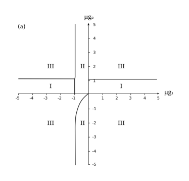
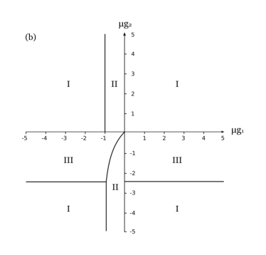
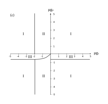
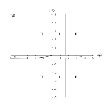
Figure 7: The $(g_{1},g_{2})$-phase portrait of the model at arbitrary fixed values of $\mu$ and for different values of the chiral chemical potential $\mu_{5}$. (a) The case $\mu_{5}=0.2\mu$. (b) The case $\mu_{5}=0.7\mu$. (c) The case $\mu_{5}=1.5\mu$. (d) The case $\mu_{5}=2.5\mu$. We use the same designations of the phases as in Fig. 1.

IV.2.2 The $(g_{1},g_{2})$-phase structure at some nontrivial values of $\mu$ and $\mu_{5}$

Let us now fix the fermion number chemical potential $\mu\neq 0$ and consider how the $(g_{1},g_{2})$-phase portrait of the model is evolved vs the chiral chemical potential $\mu_{5}$. This phase portrait at $\mu_{5}=0$ is presented in Fig. 5. In Figs. 7 we have drawn several $(g_{1},g_{2})$-phase portraits at different relations between $\mu_{5}$ and $\mu$, (a) $\mu_{5}=0.2\mu$, (b) $\mu_{5}=0.7\mu$, (c) $\mu_{5}=1.5\mu$, (d) $\mu_{5}=2.5\mu$. Analyzing Figs. 5 and 7, we see the following phase evolution of the system vs $\mu_{5}$ at fixed $\mu\neq 0$. At $\mu_{5}=0$ the SC phase III fills almost the whole $(\mu g_{1},\mu g_{2})$ plane (see Fig. 5). It means that at arbitrary fixed $g_{1}\neq 0$ and $g_{2}\neq 0$ we have superconductivity in the system at sufficiently high values of $\mu$ (see Section IV.2.1). If $\mu_{5}$ begins to grow, then for a lot of $(g_{1},g_{2})$ points there might occur a restoration of the initial symmetry (the symmetrical phase I arises) in the model. However, the further growth of $\mu_{5}$ leads to the final appearance of the CSB phase. It is the general property of the chiral chemical potential $\mu_{5}$, which promotes the chiral symmetry breaking in the system.

Since the above mentioned constraints (a),..,(d) at which Figs. 7 were drawn are not invariant under the duality transformation ${\cal D}$ (20), we would like to note that the phase portraits of Fig. 7 are not selfdual. In this case the possible duality transformation (see the previous subsubsection IV.2.1) of Figs. 7 might result in the set of four phase portraits, which are a good illustration of the evolution of the model phase structure vs the particle number chemical potential $\mu$ at arbitrary fixed $\mu_{5}\neq 0$. It is straightforwardly clear from the dual mapping of Figs. 7 that at arbitrary fixed values of $\mu_{5}>0$ and $g_{1}\neq 0$, $g_{2}\neq 0$ we have in the system the appearance of superconductivity at sufficiently high $\mu$. This property is dually conjugated to the appearing of CSB phase at sufficiently high values of $\mu_{5}$, which is a consequence of the phase portraits Fig. 7 (see the above consideration).

IV.2.3 The $(\mu,\mu_{5})$-phase structure at some nontrivial relations between $g_{1}$ and $g_{2}$

We have already considered the $(\mu,\mu_{5})$-phase structure of the model in the case of dually symmetrical constraints on the coupling constants, i.e. when $g_{1}=g_{2}$ (see Figs. 3, 4). In the present Section, special attention is paid to a more general case when $g_{1}\neq g_{2}$. Here we construct $(\mu,\mu_{5})$-phase portraits of the model for qualitatively different representative relations between $g_{1}$ and $g_{2}$. Namely, we fix in each of the regions of Fig. 1 some representative $(g_{1},g_{2})$ point and draw a corresponding $(\mu,\mu_{5})$-phase diagram. (Note that due to a duality symmetry of the model, it is sufficient to reduce the number of the representative $(g_{1},g_{2})$ points to three.)

In Fig. 8 the $(\mu,\mu_{5})$-phase portrait corresponds to arbitrary fixed $g_{1}>0$ and $g_{2}=0.2g_{1}$ (it is clear that at $\mu=\mu_{5}=0$ the point $(g_{1},g_{2}=0.2g_{1})$ lies in the symmetrical region I of Fig. 1). On the phase boundaries of this figure there are phase transitions of the second order. In Fig. 9 the $(\mu,\mu_{5})$-phase portrait corresponds to arbitrary fixed $g_{1}<0$ and $g_{2}=-2g_{1}$ (in this case at $\mu=\mu_{5}=0$ the point $(g_{1},g_{2}=-2g_{1})$ lies in the CSB region II of Fig. 1). Finally, in Fig. 10 the $(\mu,\mu_{5})$-phase portrait corresponds to arbitrary fixed $g_{1}<0$ and $g_{2}=0.5g_{1}$ (in this case at $\mu=\mu_{5}=0$ the point $(g_{1},g_{2}=0.5g_{1})$ lies in the SC region III of Fig. 1). To obtain the $(\mu,\mu_{5})$-phase portraits of the model when the point $(g_{1},g_{2})$ is fixed in the two remaining areas of Fig. 1, it is enough to perform the dual mapping of the Figs 9 and 10.

In Figs. 9, 10 all phase boundaries are the curves of the first order phase transitions, so the point T on these figures is a triple point, where three phases coexist. The main conclusion from Figs 8-10 is that the growth of $\mu_{5}$ (the growth of $\mu$) induces the chiral symmetry breaking (induces the superconductivity).

Figure 8: The $(\mu,\mu_{5})$-phase portrait of the model at arbitrary fixed $g_{1}>0$ and $g_{2}=0.2g_{1}$. The notations I, II and III are the same as in Fig. 1.

Figure 9: The $(\mu,\mu_{5})$-phase portrait of the model at arbitrary fixed $g_{1}<0$ and $g_{2}=-2g_{1}$. The notations I, II and III are the same as in Fig. 1. The letter T denotes a triple point, $\mu_{T}\approx 1/|g_{1}|$, $\mu_{5T}\approx 0.3/|g_{1}|$.

Figure 10: The $(\mu,\mu_{5})$-phase portrait of the model at arbitrary fixed $g_{1}<0$ and $g_{2}=0.5g_{1}$. The notations I, II and III are the same as in Fig. 1. The letter T denotes a triple point, $\mu_{T}\approx 1.6/|g_{1}|$, $\mu_{5T}\approx 2.2/|g_{1}|$.

V Summary and conclusions

In this paper, the duality correspondence phenomenon between CSB and SC, which was found earlier in (1+1)-dimensional 4F theories oj ; vas ; thies1 ; ekkz , is demonstrated to take place also in the framework of the (2+1)-dimensional 4F model (1). (An alternative 4F model with other dually conjugated chiral and superconducting channels of interaction is considered in Appendix B). It contains both fermion-antifermion (with $G_{1}$ a bare coupling constant) and difermion (with $G_{2}$ a bare coupling constant) interaction channels and two kinds of chemical potentials, $\mu,\mu_{5}$. The duality property of the model means that its thermodynamic potential $\Omega(M,\Delta)$ (17) is invariant under the duality transformation (20). As a result, we have established the duality correspondence between CSB and SC phases of the model (1) (as well as of the alternative model of Appendix B). Let us suppose, e.g., that for some fixed set $(g_{1},g_{2},\mu,\mu_{5})$ of external parameters (the coupling constants $g_{1}$ and $g_{2}$ are connected with bare couplings $G_{1,2}$ by the relation (31)) the chiral symmetry breaking phase is realized in the model. Then for rearranged values of external parameters, $g_{1}\leftrightarrow g_{2}$, $\mu\leftrightarrow\mu_{5}$, (or for dually conjugated set $(g_{2},g_{1},\mu_{5},\mu)$) we have the so-called dually conjugated superconducting phase (and vice versa). Moreover, it must be emphasized that the chiral condensate of the CSB phase, realized for the set $(g_{1},g_{2},\mu,\mu_{5})$, is equal to the superconducting condensate of the dually conjugated SC phase, corresponding to the set of external parameters with $g_{1}\leftrightarrow g_{2}$, $\mu\leftrightarrow\mu_{5}$ (and vice versa). In this way, it is sufficient to have the information about the ground state of the initial phase, which is realized for the set $(g_{1},g_{2},\mu,\mu_{5})$, in order to determine the properties of the ground state of the dually conjugated phase, corresponding to the rearranged external parameter set $(g_{2},g_{1},\mu_{5},\mu)$.

In order to study the role and influence of the duality property on the phase structure of the model, for comparison and illustrations, we have demonstrated a variety of phase portraits in the ($\mu,\mu_{5}$)- and $(g_{1},g_{2})$ planes. In particular, if the constraint, under which we obtain a phase portrait, is dually invariant, i.e. at $\mu=\mu_{5}$ or at $g_{1}=g_{2}$, then we have a selfdual phase diagram (see, e.g., Figs 1–4). The selfdual phase portrait is mapped into itself under the duality transformation (it is introduced in Sec. IV.2.1) , and its most characteristic feature is the mirror symmetrical arrangement of the CSB and SC phases with respect to the line $\mu=\mu_{5}$ (or $g_{1}=g_{2}$) of the phase diagram.

We have also presented a series of nonselfdual phase portraits, which do not transform into themselves under the duality mapping (see Figs. 5–10). The results obtained lead to the conclusion that the growth of the chiral chemical potential $\mu_{5}$ promotes the chiral symmetry breaking, whereas particle number chemical potential $\mu$ induces superconductivity in the system (see also in kzz ).

We hope that our investigations may shed some new light on physical effects in planar systems like high-temperature superconductors or graphene.

Appendix A Algebra of the $\gamma$ matrices in the case of SO(2,1) group

The two-dimensional irreducible representation of the (2+1)-dimensional Lorentz group SO(2,1) is realized by the following $2\times 2$ $\tilde{\gamma}$-matrices:

$$\tilde{\gamma}^{0}=\sigma_{3}=\left(\begin{array}[]{cc}1&0\\ 0&-1\end{array}\right),\,\,\tilde{\gamma}^{1}=i\sigma_{1}=\left(\begin{array}[]{cc}0&i\\ i&0\end{array}\right),\,\,\tilde{\gamma}^{2}=i\sigma_{2}=\left(\begin{array}[]{cc}0&1\\ -1&0\end{array}\right),$$ (50)

acting on two-component Dirac spinors. They have the properties:

$$Tr(\tilde{\gamma}^{\mu}\tilde{\gamma}^{\nu})=2g^{\mu\nu};~{}~{}[\tilde{\gamma}^{\mu},\tilde{\gamma}^{\nu}]=-2i\varepsilon^{\mu\nu\alpha}\tilde{\gamma}_{\alpha};~{}~{}\tilde{\gamma}^{\mu}\tilde{\gamma}^{\nu}=-i\varepsilon^{\mu\nu\alpha}\tilde{\gamma}_{\alpha}+g^{\mu\nu},$$ (51)

where $g^{\mu\nu}=g_{\mu\nu}=diag(1,-1,-1),~{}\tilde{\gamma}_{\alpha}=g_{\alpha\beta}\tilde{\gamma}^{\beta},~{}\varepsilon^{012}=1$. There is also the relation:

$$Tr(\tilde{\gamma}^{\mu}\tilde{\gamma}^{\nu}\tilde{\gamma}^{\alpha})=-2i\varepsilon^{\mu\nu\alpha}.$$ (52)

Note that the definition of chiral symmetry is slightly unusual in (2+1)-dimensions (spin is here a pseudoscalar rather than a (axial) vector). The formal reason is simply that there exists no other $2\times 2$ matrix anticommuting with the Dirac matrices $\tilde{\gamma}^{\nu}$ which would allow the introduction of a $\gamma^{5}$-matrix in the irreducible representation. The important concept of ’chiral’ symmetries and their breakdown by mass terms can nevertheless be realized also in the framework of (2+1)-dimensional quantum field theories by considering a four-component reducible representation for Dirac fields. In this case the Dirac spinors $\psi$ have the following form:

$$\psi(x)=\left(\begin{array}[]{cc}\tilde{\psi}_{1}(x)\\ \tilde{\psi}_{2}(x)\end{array}\right),$$ (55)

with $\tilde{\psi}_{1},\tilde{\psi}_{2}$ being two-component spinors. In the reducible four-dimensional spinor representation one deals with 4$\times$4 $\gamma$-matrices: $\gamma^{\mu}=diag(\tilde{\gamma}^{\mu},-\tilde{\gamma}^{\mu})$, where $\tilde{\gamma}^{\mu}$ are given in (50). One can easily show, that ($\mu,\nu=0,1,2$):

$$Tr(\gamma^{\mu}\gamma^{\nu})=4g^{\mu\nu};~{}~{}\gamma^{\mu}\gamma^{\nu}=\sigma^{\mu\nu}+g^{\mu\nu};~{}~{}$$

$$\sigma^{\mu\nu}=\frac{1}{2}[\gamma^{\mu},\gamma^{\nu}]=diag(-i\varepsilon^{\mu\nu\alpha}\tilde{\gamma}_{\alpha},-i\varepsilon^{\mu\nu\alpha}\tilde{\gamma}_{\alpha}).$$ (56)

In addition to the Dirac matrices $\gamma^{\mu}~{}~{}(\mu=0,1,2)$ there exist two other matrices, $\gamma^{3}$ and $\gamma^{5}$, which anticommute with all $\gamma^{\mu}~{}~{}(\mu=0,1,2)$ and with themselves

$$\gamma^{3}=i\left(\begin{array}[]{cc}0~{},&-I\\ I~{},&0\end{array}\right),\,\,\gamma^{5}=\left(\begin{array}[]{cc}0~{},&I\\ I~{},&0\end{array}\right),\,$$ (61)

with $I$ being the unit $2\times 2$ matrix. It is obvious that $\gamma^{3}=\gamma^{0}\gamma^{1}\gamma^{2}\gamma^{5}$ and $\gamma^{5}=-\gamma^{0}\gamma^{1}\gamma^{2}\gamma^{3}$.

Appendix B Alternative 4F (2+1)-dimensional model with dual symmetry between other CSB and SC channels

Each of the matrices $\gamma^{3}$ and $\gamma^{5}$ (see Appendix A) can be selected as a generator for the corresponding $U_{\gamma^{3}}(1)$ and $U_{\gamma^{5}}(1)$ chiral group of spinor field transformations. For example, the Lagrangian (1) is invariant with respect to $U_{\gamma^{5}}(1)$ such that $\psi_{k}(x)\to\exp(i\alpha\gamma^{5})\psi_{k}(x)$. Alternatively, it is possible to construct a 4F model with fermion-antifermion and superconducting channels, symmetric under $U_{\gamma^{3}}(1)$ continuous chiral transformations, $\psi_{k}(x)\to\exp(i\alpha\gamma^{3})\psi_{k}(x)$ ($k=1,..,N$). Its Lagrangian, e.g., reads

$$L_{\gamma^{3}}\equiv L_{\gamma^{3}}(G_{1},G_{2};\mu,\mu_{3})=\sum_{k=1}^{N}\bar{\psi}_{k}\Big{[}\gamma^{\nu}i\partial_{\nu}+\mu\gamma^{0}+\mu_{3}\gamma^{0}\gamma^{3}\Big{]}\psi_{k} + \frac{G_{1}}{N}\left(\widetilde{4F}\right)_{ch}+\frac{G_{2}}{N}\left(\widetilde{4F}\right)_{sc},$$ (62)

where the four-fermion structures $\left(\widetilde{4F}\right)_{ch}$ and $\left(\widetilde{4F}\right)_{sc}$ are used,

$$\left(\widetilde{4F}\right)_{ch}=\left(\sum_{k=1}^{N}\bar{\psi}_{k}\psi_{k}\right)^{2}+\left(\sum_{k=1}^{N}\bar{\psi}_{k}i\gamma^{3}\psi_{k}\right)^{2},~{}~{}\left(\widetilde{4F}\right)_{sc}=\left(\sum_{k=1}^{N}\psi_{k}^{T}\widetilde{C}\psi_{k}\right)\left(\sum_{j=1}^{N}\bar{\psi}_{j}\widetilde{C}\bar{\psi}_{j}^{T}\right).$$ (63)

Here $\widetilde{C}=iC\gamma^{3}\gamma^{5}$ and $\mu$ is the usual particle number chemical potential (as in (1)). Since this Lagrangian is invariant under $U_{\gamma^{3}}(1)$, there exist a corresponding conserved density of chiral charge $n_{3}=\sum_{k=1}^{N}\bar{\psi}_{k}\gamma^{0}\gamma^{3}\psi_{k}$ as well as its thermodynamically conjugate quantity, the chiral (or axial) chemical potential $\mu_{3}$. Note that in the framework of the model (62) there is also the duality between chiral and superconducting channels of interaction, i.e. between $\left(\widetilde{4F}\right)_{ch}$ and $\left(\widetilde{4F}\right)_{sc}$ four-fermion structures (63). Indeed, performing in (62)-(63) the modified Pauli-Gursey transformation of spinor fields,

$$\widetilde{PG}:~{}~{}\psi_{k}(x)\longrightarrow\frac{1}{2}(1-\gamma^{3})\psi_{k}(x)+\frac{1}{2}(1+\gamma^{3})\widetilde{C}\bar{\psi}^{T}_{k}(x),$$ (64)

we see that

$$\left(\widetilde{4F}\right)_{ch}\stackrel{{\scriptstyle\widetilde{PG}}}{{\longleftrightarrow}}\left(\widetilde{4F}\right)_{sc},~{}~{}~{}L_{\gamma^{3}}(G_{1},G_{2};\mu,\mu_{3})\stackrel{{\scriptstyle\widetilde{PG}}}{{\longleftrightarrow}}L_{\gamma^{3}}(G_{2},G_{1};-\mu_{3},-\mu).$$ (65)

The relations (65) are the basis for the duality invariance of the thermodynamic potential of the model (62).

To verify this, one can use the way of Sec. II. Indeed, the semi-bosonized version of Lagrangian (62) that contains only quadratic powers of fermionic fields and auxiliary bosonic fields $\sigma(x)$, $\tilde{\pi}(x)$, $\tilde{\Delta}(x)$ and $\tilde{\Delta}^{*}(x)$ has the following form

$${\cal L}_{\gamma^{3}}\displaystyle = \bar{\psi}_{k}\Big{[}\gamma^{\nu}i\partial_{\nu}+\mu\gamma^{0}+\mu_{3}\gamma^{0}\gamma^{3}-\sigma-i\gamma^{3}\tilde{\pi}\Big{]}\psi_{k}-\frac{N(\sigma^{2}+\tilde{\pi}^{2})}{4G_{1}}$$ (66)

$$~{}~{}~{}~{}~{}~{}~{}~{}~{}~{}~{}~{}~{}~{}~{}~{}~{}-\frac{N}{4G_{2}}\tilde{\Delta}^{*}\tilde{\Delta}-\frac{\tilde{\Delta}^{*}}{2}[\psi_{k}^{T}\widetilde{C}\psi_{k}]-\frac{\tilde{\Delta}}{2}[\bar{\psi}_{k}\widetilde{C}\bar{\psi}_{k}^{T}]$$

(in (66) and below the summation over $k=1,...,N$ is implied). On Euler-Lagrange equations for bosonic fields,

$$\sigma(x)=-2\frac{G_{1}}{N}(\bar{\psi}_{k}\psi_{k}), \tilde{\pi}(x)=-2\frac{G_{1}}{N}(\bar{\psi}_{k}i\gamma^{3}\psi_{k}),~{}~{}$$

$$\tilde{\Delta}(x)=-2\frac{G_{2}}{N}(\psi_{k}^{T}\widetilde{C}\psi_{k}), \tilde{\Delta}^{*}(x)=-2\frac{G_{2}}{N}(\bar{\psi}_{k}\widetilde{C}\bar{\psi}_{k}^{T}),$$ (67)

the semi-bosonized Lagrangian (66) is equivalent to the 4F Lagrangian (62). Note also that the bosonic fields $\tilde{\Delta}(x)$ and $\tilde{\Delta}^{*}(x)$ are pseudoscalars, whereas $\sigma(x)$ and $\tilde{\pi}(x)$ are scalars with respect to parity transformation (9).

Then, the thermodynamic potential $\Omega_{\gamma^{3}}(M,\Delta)$, which describes the ground state of the model (62)-(66), is analogously defined by the following relation (for convenience, we omit here and below the tilde in fields)

$$\int d^{3}x\Omega_{\gamma^{3}}(M,\Delta)\,\, = \,\,\int d^{3}x\left(\frac{M^{2}}{4G_{1}}+\frac{\Delta^{2}}{4G_{2}}\right)+\frac{i}{N}\ln\left(\int\prod_{l=1}^{N}[d\bar{\psi}_{l}][d\psi_{l}]\exp\Big{(}i\int d^{3}x\Big{[}\bar{\psi}_{k}D_{\gamma^{3}}\psi_{k}\right.$$ (68)

$$\left.-\frac{\Delta}{2}(\psi_{k}^{T}\widetilde{C}\psi_{k})-\frac{\Delta}{2}(\bar{\psi}_{k}\widetilde{C}\bar{\psi}_{k}^{T})\Big{]}\Big{)}\right),$$

where $D_{\gamma^{3}}=\gamma^{\rho}i\partial_{\rho}+\mu\gamma^{0}+\mu_{3}\gamma^{0}\gamma^{3}-M$. In writing down this expression, we used the same arguments that were used in the derivation of the thermodynamic potential in the framework of the model (1) (see the derivation of (16) in Section II). Path integration in the expression (68) is evaluated in Appendix C so we have for the TDP (68) the following expression

$$\Omega_{\gamma^{3}}(M,\Delta) = \frac{M^{2}}{4G_{1}}+\frac{\Delta^{2}}{4G_{2}}+\frac{i}{2}\int\frac{d^{3}p}{(2\pi)^{3}}\ln\Big{[}\tilde{\lambda}_{1}(p)\tilde{\lambda}_{2}(p)\tilde{\lambda}_{3}(p)\tilde{\lambda}_{4}(p)\Big{]},$$ (69)

where $\tilde{\lambda}_{1,...,4}(p)$ are presented in (82). Comparing this thermodynamic potential with the TDP $\Omega(M,\Delta)$ (17) of the model (1), we see that

$$\Omega_{\gamma^{3}}(M,\Delta) = \Omega(M,\Delta)\Big{|}_{\mu_{5}\to\mu_{3}}.$$ (70)

As a result, it is clear that the TDP $\Omega_{\gamma^{3}}(M,\Delta)$ of the 4F model (62) is invariant under the following dual transformation

$$G_{1}\longleftrightarrow G_{2},~{}~{}M\longleftrightarrow\Delta,~{}~{}\mu\longleftrightarrow\mu_{3}.$$ (71)

Furthermore, to find phase portraits of the model (62), it is sufficient to perform in all Figs 1,..,10 the replacement $\mu_{5}\to\mu_{3}$.

Appendix C The path integration over anticommuting fields

Let us calculate the following path integral over anticommuting four-component Dirac spinor fields $\psi(x)$, $\bar{\psi}(x)$:

$$I_{\Gamma}=\int[d\bar{\psi}][d\psi]\exp\Big{(}i\int d^{3}x\Big{[}\bar{\psi}D_{\Gamma}\psi-\frac{\Delta}{2}(\psi^{T}C\Gamma\psi)-\frac{\Delta}{2}(\bar{\psi}C\Gamma\bar{\psi}^{T})\Big{]}\Big{)},$$ (72)

where $C$ is the charge conjugation matrix, $C=\gamma^{2}$. Since in the 4$\times$4 spinor space the product matrix $C\Gamma$ should be an antisymmetric one, it is clear that the $\Gamma$ matrix in (72) might be, e.g., the unit matrix ${\bf 1_{s}}$ in the spinor space or $\Gamma=i\gamma^{3}\gamma^{5}$ (for notations see Appendix A), etc. Note in addition that at $\Gamma={\bf 1_{s}}$ and $D_{\Gamma}=D$ (see in (16)) the integral $I_{\Gamma}$ is equal to the argument of the $\ln$-function in the formula (16) in the particular case $N=1$, whereas at $\Gamma=i\gamma^{3}\gamma^{5}$ and $D_{\Gamma}=D_{\gamma^{3}}$ (see (68)) the integral $I_{\Gamma}$ is equal to the argument of the $\ln$-function in the formula (68) also in the particular case $N=1$. Recall, there are general Gaussian path integrals vasiliev :

$$\int[d\psi]\exp\Big{(}i\int d^{3}x\Big{[}-\frac{1}{2}\psi^{T}A\psi+\eta^{T}\psi\Big{]}\Big{)} = \left(\det(A)\right)^{1/2}\exp\Big{(}-\frac{i}{2}\int d^{3}x\Big{[}\eta^{T}A^{-1}\eta\Big{]}\Big{)},$$ (73)

$$\int[d\bar{\psi}]\exp\Big{(}i\int d^{3}x\Big{[}-\frac{1}{2}\bar{\psi}A\bar{\psi}^{T}+\bar{\eta}\bar{\psi}^{T}\Big{]}\Big{)} = \left(\det(A)\right)^{1/2}\exp\Big{(}-\frac{i}{2}\int d^{3}x\Big{[}\bar{\eta}A^{-1}\bar{\eta}^{T}\Big{]}\Big{)},$$ (74)

where $A$ is an antisymmetric operator in coordinate and spinor spaces, and $\eta(x)$, $\bar{\eta}(x)$ are anticommuting spinor sources which also anticommute with $\psi$ and $\bar{\psi}$. First, let us integrate in (72) over $\psi$-fields with the help of the relation (73) supposing there that $A=\Delta C\Gamma$, $\bar{\psi}D_{\Gamma}=\eta^{T}$, i.e. $\eta=D_{\Gamma}^{T}\bar{\psi}^{T}$. Then

$$I_{\Gamma}=\left(\det(\Delta C\Gamma)\right)^{1/2}\int[d\bar{\psi}]\exp\Big{(}-\frac{i}{2}\int d^{3}x\bar{\psi}\big{[}\Delta C\Gamma+D_{\Gamma}(\Delta C\Gamma)^{-1}D_{\Gamma}^{T}\big{]}\bar{\psi}^{T}\Big{)}.$$ (75)

Second, the integration over $\bar{\psi}$-fields in (75) can be easily performed with the help of the formula (74), where one should put $A=\Delta C\Gamma+D_{\Gamma}(\Delta C\Gamma)^{-1}D_{\Gamma}^{T}$ and $\bar{\eta}=0$. As a result, we have

$$I_{\Gamma}=\left(\det(\Delta C\Gamma)\right)^{1/2}\left(\det[\Delta C\Gamma+D_{\Gamma}(\Delta C\Gamma)^{-1}D_{\Gamma}^{T}]\right)^{1/2}=\left(\det[\Delta^{2}(C\Gamma)^{2}+D_{\Gamma}(C\Gamma)^{-1}D_{\Gamma}^{T}C\Gamma]\right)^{1/2}.$$ (76)

We evaluate the expression (76) in two cases, (i) when $\Gamma={\bf 1_{s}}$ and $D_{\Gamma}=D$, where $D$ is presented in (16), and (ii) when $\Gamma=i\gamma^{3}\gamma^{5}$ and $D_{\Gamma}=D_{\gamma^{3}}$, where $D_{\gamma^{3}}$ is given in (68).

(i) The case $\Gamma={\bf 1_{s}}$ and $D_{\Gamma}=D=\gamma^{\rho}i\partial_{\rho}+\mu\gamma^{0}+\mu_{5}\gamma^{0}\gamma^{5}-M$. Taking into account the relations $(\partial_{\nu})^{T}=-\partial_{\nu}$ and $C^{-1}(\gamma^{\nu})^{T}C=-\gamma^{\nu}$ ($\nu=0,1,2$), we obtain from (76)

$$I_{{\bf 1_{s}}}=\left(\det[-\Delta^{2}+D_{+}D_{-}]\right)^{1/2}\equiv\left(\det B\right)^{1/2},$$ (77)

where $D_{\pm}=\gamma^{\nu}i\partial_{\nu}-M\pm(\mu\gamma^{0}+\mu_{5}\gamma^{0}\gamma^{5})$. Using the general relation $\det B=\exp({\rm Tr}\ln B)$, we get from (77):

$$\ln I_{{\bf 1_{s}}}=\frac{1}{2}{\rm Tr}\ln\left(B\right)=\frac{1}{2}\sum_{i=1}^{4}\int\frac{d^{3}p}{(2\pi)^{3}}\ln(\lambda_{i}(p))\int d^{3}x.$$ (78)

(A more detailed consideration of operator traces is presented in Appendix A of the paper Ebert:2009ty .) In this formula the symbol Tr means the trace of an operator both in the coordinate and internal spaces. Moreover, $\lambda_{i}(p)$ ($i=1,...,4$) in (78) are four eigenvalues of the 4$\times$4 Fourier transformation matrix $\bar{B}(p)$ of the operator $B$ from (77). Namely,

$$\lambda_{1,...,4}(p) = M^{2}-|\vec{p}|^{2}+p_{0}^{2}-\mu^{2}+\mu_{5}^{2}-\Delta^{2}\pm 2\sqrt{M^{2}(p_{0}^{2}-|\vec{p}|^{2})+(|\mu||\vec{p}|\pm|\mu_{5}|p_{0})^{2}},$$ (79)

where $|\vec{p}|=\sqrt{p_{1}^{2}+p_{2}^{2}}$. It is clear from these relations that $\lambda_{1,...,4}(p)$ are even functions vs $\mu$ and/or $\mu_{5}$. So, it is enough to take into account only nonnegative values of the chemical potentials $\mu$ and $\mu_{5}$.

(ii) The case $\Gamma=i\gamma^{3}\gamma^{5}$ and $D_{\Gamma}=D_{\gamma^{3}}=\gamma^{\rho}i\partial_{\rho}+\mu\gamma^{0}+\mu_{3}\gamma^{0}\gamma^{3}-M$. In this case $C^{-1}D_{\Gamma}^{T}C=\gamma^{\rho}i\partial_{\rho}-\mu\gamma^{0}+\mu_{3}\gamma^{0}\gamma^{3}-M$. Then it follows from (76) that

$$I_{\Gamma}=\left(\det[-\Delta^{2}+\tilde{D}_{+}\tilde{D}_{-}]\right)^{1/2}\equiv\left(\det{\cal B}\right)^{1/2},$$ (80)

where $\tilde{D}_{\pm}=\gamma^{\nu}i\partial_{\nu}-M\pm(\mu\gamma^{0}+\mu_{3}\gamma^{0}\gamma^{3})$. Then, similar to (78), it is easy to find that in the case under consideration

$$\ln I_{\Gamma}=\frac{1}{2}{\rm Tr}\ln\left({\cal B}\right)=\frac{1}{2}\sum_{i=1}^{4}\int\frac{d^{3}p}{(2\pi)^{3}}\ln(\tilde{\lambda}_{i}(p))\int d^{3}x,$$ (81)

where $\tilde{\lambda}_{i}(p)$ ($i=1,...,4$) are four eigenvalues of the 4$\times$4 Fourier transformation matrix $\bar{\cal B}(p)$ of the operator ${\cal B}$ from (80). It turns out that the eigenvalues $\tilde{\lambda}_{i}(p)$ are connected with the eigenvalues $\lambda_{i}(p)$ (79) by the simple relations

$$\tilde{\lambda}_{i}(p)=\lambda_{i}(p)\Big{|}_{\mu_{5}\to\mu_{3}}.$$ (82)

Appendix D Evaluation of the function $F_{1}(M)$ (38).

To calculate the improper convergent integral in (38) we first use there a polar coordinate system, i.e. $\int d^{2}p=2\pi\int_{0}^{\infty}pdp$, and then restrict the $p$-integration region by $\Lambda$ (suppose in addition that $\Lambda>>\mu,\mu_{5},M$). As a result, we come to the regularized expression $F_{1\Lambda}(M)$ of the TDP (38), $F_{1\Lambda}(M)=V_{1}(M)+I_{1}+I_{+}+I_{-}$, where

$$I_{1} = -\int_{0}^{\Lambda}\frac{pdp}{2\pi}\Big{[}\sqrt{M^{2}+(p+\mu_{5})^{2}}+\sqrt{M^{2}+(p-\mu_{5})^{2}}-2\sqrt{p^{2}+M^{2}}\Big{]},$$ (83)

$$I_{\pm} = -\int_{0}^{\Lambda}\frac{pdp}{2\pi}\left(\mu-\sqrt{M^{2}+(p\pm\mu_{5})^{2}}\right)\theta\left(\mu-\sqrt{M^{2}+(p\pm\mu_{5})^{2}}\right).$$ (84)

Due to the presence of the $\theta(x)$-functions in (84) and sufficiently high values of the cutoff parameter $\Lambda>>\mu,\mu_{5},M$, the quantities $I_{\pm}$ indeed do not depend on $\Lambda$. Moreover, it is evident that $I_{+}$ is a nonzero quantity only in the case $\mu>\sqrt{M^{2}+\mu_{5}^{2}}$. Hence, substituting $q=p+\mu_{5}$ for the $I_{+}$-integration in (84), we have

$$I_{+} = -\frac{\theta\left(\mu-\sqrt{M^{2}+\mu_{5}^{2}}\right)}{2\pi}\int_{\mu_{5}}^{\sqrt{\mu^{2}-M^{2}}}(q-\mu_{5})\left(\mu-\sqrt{M^{2}+q^{2}}\right)dq$$ (85)

(The upper limit in the integral (85) corresponds to a value of the momentum $p$, where the $\theta$-function of the integrand for $I_{+}$ from (84) is equal to zero, i.e. to a value of $p$ determined by the condition $\mu=\sqrt{M^{2}+(p+\mu_{5})^{2}}$.)

It is convenient to present the quantity $I_{-}$ from (84) as a sum of two integrals, $I_{-}=i_{1}+i_{2}$, where

$$i_{1} = -\int_{0}^{\mu_{5}}\frac{pdp}{2\pi}\left(\mu-\sqrt{M^{2}+(p-\mu_{5})^{2}}\right)\theta\left(\mu-\sqrt{M^{2}+(p-\mu_{5})^{2}}\right),$$ (86)

$$i_{2} = -\int^{\Lambda}_{\mu_{5}}\frac{pdp}{2\pi}\left(\mu-\sqrt{M^{2}+(p-\mu_{5})^{2}}\right)\theta\left(\mu-\sqrt{M^{2}+(p-\mu_{5})^{2}}\right).$$ (87)

It is clear that $i_{2}$ is a nonzero quantity only at $\mu>M$. Then, performing in the integral (87) the substitution $q=p-\mu_{5}$, we obtain

$$i_{2} = -\frac{\theta\left(\mu-M\right)}{2\pi}\int_{0}^{\sqrt{\mu^{2}-M^{2}}}(q+\mu_{5})\left(\mu-\sqrt{M^{2}+q^{2}}\right)dq.$$ (88)

Obviously, we have $i_{1}\equiv 0$ at $\mu<M$. To evaluate $i_{1}$ at other values of $\mu$, we should, first, substitute $q=\mu_{5}-p$ in the integral (86) and then consider two different regions of the parameter $\mu$, (i) $\omega_{1}=\{\mu:M<\mu<\sqrt{M^{2}+\mu_{5}^{2}}\}$, (ii) $\omega_{2}=\{\mu:\sqrt{M^{2}+\mu_{5}^{2}}<\mu\}$. As a result, we have

$$i_{1} = -\frac{\theta\left(\mu-M\right)\theta\left(\sqrt{M^{2}+\mu_{5}^{2}}-\mu\right)}{2\pi}\int_{0}^{\sqrt{\mu^{2}-M^{2}}}(\mu_{5}-q)\left(\mu-\sqrt{M^{2}+q^{2}}\right)dq$$ (89)

$$-\frac{\theta\left(\mu-\sqrt{M^{2}+\mu_{5}^{2}}\right)}{2\pi}\int_{0}^{\mu_{5}}(\mu_{5}-q)\left(\mu-\sqrt{M^{2}+q^{2}}\right)dq.$$

Summing the expressions (85), (88) and (89), we have

$$I_{+}+I_{-}=-\frac{\mu_{5}\theta\left(\mu-M\right)\theta\left(\sqrt{M^{2}+\mu_{5}^{2}}-\mu\right)}{\pi}\int_{0}^{\sqrt{\mu^{2}-M^{2}}}\left(\mu-\sqrt{M^{2}+q^{2}}\right)dq$$

$$-\frac{\theta\left(\mu-\sqrt{M^{2}+\mu_{5}^{2}}\right)}{\pi}\left\{\mu_{5}\int_{0}^{\mu_{5}}\left(\mu-\sqrt{M^{2}+q^{2}}\right)dq+\int_{\mu_{5}}^{\sqrt{\mu^{2}-M^{2}}}\left(\mu-\sqrt{M^{2}+q^{2}}\right)qdq\right\}.$$ (90)

To calculate the $I_{1}$-term of the regularized TDP $F_{1\Lambda}(M)$, it is useful to present $I_{1}$ as a sum of three integrals, each one corresponds to some square root expression of the integrand in (83). Then, substituting $q=p+\mu_{5}$ and $q=p-\mu_{5}$ in two of these integrals, it is possible to present $I_{1}$ in the form

$$-2\pi I_{1} = \left(\int^{0}_{\mu_{5}}+\int_{0}^{\Lambda}+\int_{\Lambda}^{\Lambda+\mu_{5}}\right)(q-\mu_{5})\sqrt{q^{2}+M^{2}}dq-2\int_{0}^{\Lambda}q\sqrt{q^{2}+M^{2}}dq$$ (91)

$$~{}~{}~{}~{}~{}~{}~{}~{}~{}~{}~{}~{}+\left(\int^{0}_{-\mu_{5}}+\int_{0}^{\Lambda}+\int_{\Lambda}^{\Lambda-\mu_{5}}\right)(q+\mu_{5})\sqrt{q^{2}+M^{2}}dq$$

$$= 2\int_{0}^{\mu_{5}}(\mu_{5}-q)\sqrt{q^{2}+M^{2}}dq+\int_{\Lambda}^{\Lambda+\mu_{5}}(q-\mu_{5})\sqrt{q^{2}+M^{2}}dq+\int_{\Lambda}^{\Lambda-\mu_{5}}(q+\mu_{5})\sqrt{q^{2}+M^{2}}dq.$$

Since $\Lambda>>\mu,\mu_{5},\Delta$, we an use $\sqrt{q^{2}+\Delta^{2}}=q+\Delta^{2}/(2q)+\cdots$ in the last two terms of (91). Then, after integrations one can see that the sum of these two last integrals in (91) is equal to zero in the limit $\Lambda\to\infty$. Hence,

$$\lim_{\Lambda\to\infty}I_{1} = -\frac{1}{\pi}\int_{0}^{\mu_{5}}dq(\mu_{5}-q)\sqrt{q^{2}+M^{2}}=-\frac{M^{3}}{3\pi}+\frac{(\mu_{5}^{2}+M^{2})\sqrt{\mu_{5}^{2}+M^{2}}}{3\pi}$$ (92)

$$-\frac{\mu_{5}^{2}\sqrt{\mu_{5}^{2}+M^{2}}}{2\pi}-\frac{\mu_{5}M^{2}}{2\pi}\ln\left[\frac{\mu_{5}+\sqrt{\mu_{5}^{2}+M^{2}}}{M}\right].$$

Finally, performing in (90) trivial table integrations and using the relation

$$F_{1}(M)=\lim_{\Lambda\to\infty}F_{1\Lambda}(M)=V_{1}(M)+\lim_{\Lambda\to\infty}I_{1}+I_{+}+I_{-},$$ (93)

we obtain from (93), (90) and (92) the expression (40) (the function $V_{1}(M)$ is given in the text below (39)).

References

• (1) D. Ebert and M.K. Volkov, Z. Phys. C 16, 205 (1983); D. Ebert, H. Reinhardt and M.K. Volkov, Prog. Part. Nucl. Phys.  33, 1 (1994).
• (2) M. Buballa, Phys. Rept.  407, 205 (2005).
• (3) Y. Nambu and G. Jona-Lasinio, Phys. Rev.122, 345 (1961); Phys. Rev. 124, 246 (1961).
• (4) D.J. Gross and A. Neveu, Phys. Rev. D 10, 3235 (1974).
• (5) I.V. Krive and A.S. Rozhavsky, Sov. Phys. Usp.  30, 370 (1987) [Usp. Fiz. Nauk 152, 33 (1987)].
• (6) A.J. Heeger, S. Kivelson, J.R. Schrieffer , and W.-P. Su, Rev. Mod. Phys. 60, 781 (1988).
• (7) A. Chodos and H. Minakata, Phys. Lett. A 191, 39 (1994); Lect. Notes Phys.  508, 231 (1998) [hep-th/9709197]; H. Caldas, J.L. Kneur, M.B. Pinto and R.O. Ramos, Phys. Rev.  B 77, 205109 (2008).
• (8) V. Schön and M. Thies, At the Frontier of Particle Physics: Handbook of QCD: ”Boris Ioffe Festschrift”, Vol. 3, 1945, World Scientific (2001) [hep-th/0008175]; M. Thies, J. Phys. A 39, 12707 (2006).
• (9) G.W. Semenoff, I.A. Shovkovy and L.C.R. Wijewardhana, Mod. Phys. Lett. A 13, 1143 (1998).
• (10) V.C. Zhukovsky, K.G. Klimenko, V.V. Khudyakov and D. Ebert, JETP Lett.  73, 121 (2001); V.C. Zhukovsky and K.G. Klimenko, Theor. Math. Phys.  134, 254 (2003); E.J. Ferrer, V.P. Gusynin and V. de la Incera, Mod. Phys. Lett. B 16, 107 (2002); Eur. Phys. J. B 33, 397 (2003).
• (11) E.C. Marino and L.H.C.M. Nunes, Nucl. Phys. B 741, 404 (2006); L.H.C.M. Nunes, R.L.S. Farias and E.C. Marino, Phys. Lett. A 376, 779 (2012).
• (12) K.G. Klimenko, R.N. Zhokhov and V.C. Zhukovsky, Phys. Rev. D 86, 105010 (2012).
• (13) K.G. Klimenko, R.N. Zhokhov and V.C. Zhukovsky, Mod. Phys. Lett. A 28, 1350096 (2013).
• (14) D. Mesterhazy, J. Berges, and L. von Smekal, Phys. Rev. B 86, 245431 (2012).
• (15) D. Ebert, K.G. Klimenko, P.B. Kolmakov and V.C. Zhukovsky, arXiv:1509.08093 [cond-mat.mes-hall].
• (16) K.G. Klimenko, Z. Phys. C 37, 457 (1988); B. Rosenstein, B.J. Warr, and S.H. Park, Phys. Rev. D 39, 3088 (1989); Phys. Rev. Lett. 62, 1433 (1989).
• (17) G.W. Semenoff and L.C.R. Wijewardhana, Phys. Rev. Lett. 63, 2633 (1989); Phys. Rev. D 45, 1342 (1992).
• (18) B. Rosenstein, B.J. Warr and S.H. Park, Phys. Rept.  205, 59 (1991).
• (19) K.G. Klimenko, Z. Phys. C 54, 323 (1992); Theor. Math. Phys.  89, 1161 (1992); Theor. Math. Phys.  90, 1 (1992); V.P. Gusynin, V.A. Miransky and I.A. Shovkovy, Phys. Rev. Lett.  73, 3499 (1994); A.S. Vshivtsev, B.V. Magnitsky and K.G. Klimenko, Phys. Atom. Nucl.  57, 2171 (1994); Theor. Math. Phys.  106, 319 (1996); V.P. Gusynin, D.K. Hong and I.A. Shovkovy, Phys. Rev. D 57, 5230 (1998).
• (20) A. Chodos, H. Minakata, F. Cooper, A. Singh, and W. Mao, Phys. Rev. D 61, 045011 (2000).
• (21) D. Ebert, K.G. Klimenko and H. Toki, Phys. Rev. D 64, 014038 (2001); H. Kohyama, Phys. Rev. D 77, 045016 (2008); Phys. Rev. D 78, 014021 (2008).
• (22) D. Ebert, K.G. Klimenko, A.V. Tyukov and V.C. Zhukovsky, Phys. Rev. D 78, 045008 (2008); D. Ebert, K.G. Klimenko, Phys. Rev.  D80, 125013 (2009); D. Ebert, N.V. Gubina, K.G. Klimenko, S.G. Kurbanov and V.C. Zhukovsky, Phys. Rev. D 84, 025004 (2011).
• (23) N.V. Gubina, K.G. Klimenko, S.G. Kurbanov and V.C. Zhukovsky, Phys. Rev. D 86, 085011 (2012); Moscow Univ. Phys. Bull.  67, 131 (2012).
• (24) J.-L. Kneur, M.B. Pinto, R.O. Ramos and E. Staudt, Phys. Rev. D 76, 045020 (2007); Phys. Lett. B 657, 136 (2007).
• (25) K.G. Klimenko, Z. Phys. C 50, 477 (1991); Mod. Phys. Lett. A 9, 1767 (1994).
• (26) I. Ojima and R. Fukuda, Prog. Theor. Phys.  57, 1720 (1977).
• (27) A.N. Vasiliev and G.Y. Panasyuk, Theor. Math. Phys.  103, 570 (1995) [Teor. Mat. Fiz.  103, 295 (1995)].
• (28) M. Thies, Phys. Rev. D 68, 047703 (2003); Phys. Rev. D 90, no. 10, 105017 (2014).
• (29) D. Ebert, T.G. Khunjua, K.G. Klimenko and V.C. Zhukovsky, Phys. Rev. D 90, 045021 (2014).
• (30) N.D. Mermin and H. Wagner, Phys. Rev. Lett. 17, 1133 (1966); S. Coleman, Commun. Math. Phys. 31, 259 (1973).
• (31) A.A. Andrianov, D. Espriu and X. Planells, Eur. Phys. J. C 73, 2294 (2013); Eur. Phys. J. C 74, 2776 (2014); R. Gatto and M. Ruggieri, Phys. Rev. D 85, 054013 (2012); M. Ruggieri, arXiv:1110.4907; L. Yu, H. Liu and M. Huang, Phys. Rev. D 90, 074009 (2014); L. Yu, H. Liu and M. Huang, arXiv:1511.03073 [hep-ph]; G. Cao and P. Zhuang, Phys. Rev. D 92, 105030 (2015).
• (32) V.V. Braguta and A.Y. Kotov, arXiv:1601.04957 [hep-th].
• (33) V.A. Miransky and I.A. Shovkovy, Phys. Rept.  576, 1 (2015).
• (34) K. Fukushima, D.E. Kharzeev, H.J. Warringa, Phys. Rev. D 78, 074033 (2008).
• (35) A.J. Mizher, A. Raya and C. Villavicencio, Int. J. Mod. Phys. B 30, 1550257 (2015).
• (36) S. Ryu, C. Mudry, C.-Y. Hou, and C. Chamon, Phys. Rev. B 80, 205319 (2009).
• (37) W. Pauli, Nuovo Cimento, 6, 204 (1957); F. Gürsey, Nuovo Cimento, 7, 411, (1957).
• (38) V.C. Zhukovsky, K.G. Klimenko and V.V. Khudyakov, Theor. Math. Phys.  124, 1132 (2000) [Teor. Mat. Fiz.  124, 323 (2000)].
• (39) B. Vanderheyden and A.D. Jackson, Phys. Rev. D 61, 076004 (2000); V.C. Zhukovsky, V.V. Khudyakov, K.G. Klimenko and D. Ebert, JETP Lett.  74, 523 (2001) [Pisma Zh. Eksp. Teor. Fiz.  74, 595 (2001)].
• (40) G. Cao, L. He and P. Zhuang, Phys. Rev. D 90, 056005 (2014).
• (41) A.N. Vasiliev,“Functional methods in quantum field theory and statistical physics”, Leningrad Univ. Press, Leningrad, 1976.
• (42) D. Ebert, K.G. Klimenko, Phys. Rev.  D80, 125013 (2009).