The evolution of Brown-York quasilocal energy due to evolution of Lovelock gravity in a system of M0-branes

Abstract

Recently, it has been suggested in [JHEP 12(2015)003] that the Brown-York mechanism can be used to measure the quasilocal energy in Lovelock gravity. We have used this method in a system of M0-branes and show that the Brown-York energy evolves in the process of birth and growth of Lovelock gravity. This can help us to predict phenomenological events which are emerged as due to dynamical structure of Lovelock gravity in our universe. In this model, first, M0-branes join to each other and form an M3-brane and an anti-M3-branes connected by an M2-brane. This system is named BIon. Universes and anti-universes live on M3-branes and M2 plays the role of wormhole between them. By passing time, M2 dissolves in M3’s and nonlinear massive gravities, like Lovelock massive gravity, emerges and grows. By closing M3-branes, BIon evolves and wormhole between branes makes a transition to black hole. During this stage, Brown-York energy increases and shrinks to large values at the colliding points of branes. By approaching M3-branes towards each other, the square energy of their system becomes negative and some tachyonic states are produced. To remove these states, M3-branes compact, the sign of compacted gravity changes, anti-gravity is created which leads to getting away of branes from each other. Also, the Lovelock gravity disappears and it’s energy forms a new M2 between M3-branes. By getting away of branes from each other, Brown-York energy decreases and shrinks to zero.

PACS numbers: 11.25.Tq, 03.65.Ud, 98.80.-k, 04.50.Gh, 11.25.Yb, 98.80.Qc
Keywords: Brown-York energy, Wormhole, BIonic system, $M2$ and $M5$-Branes

I Introduction

Measuring the quasilocal energy in general relativity is an extremely important but a long eluding problem. There is an ambiguity in calculating this energy as due to its nonlinear nature and the fact that gravitational energy is non-localizable. The best method for measuring gravitational energy has been proposed by the Brown and York in m1 by employing the Hamilton-Jacob theory for gravitation. This method has been studied extensively in general relativity for static spacetime with spherical symmetry and also for Kerr black hole s1 ; s2 ; s3 ; s4 . Recently, It has been generalized the Brown-York formalism to all orders in Lovelock gravity and have been verified the conjunction for pure Lovelock black hole s5 . Motivated by this research, we investigate the evolution of this energy during the birth and growth of Lovelock gravity in a system of M0-branes. In our model, M0-branes join to each other and form universe and anti-universe which are connected by a wormhole. This system is named BIon. By considering the changes in Brown-York energy, we can predict the evolution of Lovelock gravity in a BIonic system. This can help us predict phenomenological events which are emerged due to dynamical structure of Lovelock gravity in our universe.

In previous work, BIon model m3 ; m4 ; m5 ; m6 ; m7 ; m8 has been used in cosmology to consider the evolution of universe from birth and then inflation to late time acceleration. For example, in one paper, k black fundamental strings link to each other and construct a BIon m3 ; m4 . Coincidence with the birth of BIon, a universe and an anti-universe are born which are connected with each other through a wormhole m3 ; m4 . This wormhole dissolves in branes and causes their expansion. In another work, first, N fundamental strings transit to N pair of M0 and anti-M0-branes. Then, M0-branes glue to each other and build a pair of an M5 and an anti-M5-brane. This pair decays to an M3-brane, an anti-M3-brane in additional to one M2-brane. Our universe is formed on one of these M3-branes and M2 has the role of wormhole . In this theory, there is not any big-bang and the origin of universe is a fundamental string m7 . In another scenario, first M0-branes are compacted on a circle and N D0-branes are created. Then, N D0-branes join to each other and build one D5-branes. Next, D5- brane is compacted on two circles and a D3-brane, two D1-brane and some extra energies are produced. Our universe is built on D3-brane and D1-branes dissolve in universe and lead to inflation and late time acceleration m8 .

Now, a natural question arises to how can we consider the evolution of BIon in four dimensional universe? We answer it by measuring the Brown-York energy which changes by changing the Lovelock gravity in this system. In our consideration, first M0-branes join to each other and build an M3, an anti-M3 and an M2-brane which connects them. Each of universes live on an M3-brane and M2 has the role of wormhole. By passing time, this M2 dissolves into M3-branes, some nonlinear gravities like the $F(R)$-gravity and Love-lock gravity m2 ; mm2 emerge and universe expands. By closing branes towards each other, wormhole becomes more thermal and transits to black hole. During this era, the Brown-York energy increases and shrinks to large values. By approaching branes to each other, the square energy of their system becomes negative and some tachyonic states are produced. To remove these states, M3 compacts, the sign of compacted gravity changes and the anti-gravity emerges which leads to getting away of branes from each other and contraction of universe. In this epoch, the Brown-York energy decreases and shrinks to zero.

The outline of the paper is the following. In section II, we consider the evolution of the Brown-York energy during the expansion branch in BIonic system. In section III, we discuss as to how by compacting branes gravity changes to anti- gravity and the particles get away from each other. This leads to a decrease of the Brown-York energy in BIonic system. The last section is devoted to discussion and conclusions.

II the evolution of the Brown-York energy during the expansion branch in BIonic system

In this section, we show that the relevant action of Mp-branes can be obtained by summing over the actions of p M0-branes. Then, we obtain the Brown-York energy in a system of M2-M3 branes. In this system, universes are placed on M3-branes and connect with each other via an M2-brane. M2 plays the role of wormhole, dissolves in M3-branes and leads to the emergence of nonlinear gravity and a black hole. In the background of this gravity, the Brown-York energy increases and tends to large values. It has been shown that the Brown-York energy can be obtained from following equation m1 :

$$E_{BY}=\frac{1}{8\pi}\int_{\beta}d^{2}x\sqrt{q}(\tilde{k}-\tilde{k}_{0})$$ (1)

where q is the metric defined on the surface $B$ which is the boundary of three space $\Sigma$ and $\tilde{k}_{0}$ denotes the trace of extrinsic curvature for some reference spacetime. We will use of this equation and consider the evolution of energy in BIon. To begin considering the evolution of energy in BIon, we should first consider the process of formation of BIon in M-theory. To this end, we should construct the action of BIon from D1 and M1-branes and also show that these branes are built of D0 and M0-brane. We introduce the Lagrangian for D1 as m7 ; m8 ; m9 ; m10 ; m11 ; m12 ; m13 ; m14 :

$$S=-T_{D1}\int d^{2}\sigma~{}STr\Bigg{(}-det(P_{ab}[E_{mn}E_{mi}(Q^{-1}+\delta)^{ij}E_{jn}])det(Q^{i}_{j})\Bigg{)}^{1/2}~{}~{}$$ (2)

where

$$E_{mn}=G_{mn}+B_{mn},\qquad Q^{i}_{j}=\delta^{i}_{j}+i\lambda[X^{j},X^{k}]E_{kj}$$ (3)

where $\lambda=2\pi l_{s}^{2}$, $G_{ab}=\eta_{ab}+\partial_{a}X^{i}\partial_{b}X^{i}$ and $X^{i}$ are scalar fields of mass dimension. Here $a,b=0,1,...,p$ are the world-volume indices of the Dp-branes, $i,j,k=p+1,...,9$ are indices of the transverse space, and m,n are the ten-dimensional spacetime indices. Also, $T_{Dp}=\frac{1}{g_{s}(2\pi)^{p}l_{s}^{p+1}}$ is the tension of Dp-brane, $l_{s}$ is the string length and $g_{s}$ is the string coupling. To obtain the Lagrangian for Dp-brane, we should use of following rules m7 ; m8 :

$$\Sigma_{a=0}^{p}\Sigma_{m=0}^{9}\rightarrow\frac{1}{(2\pi l_{s})^{p}}\int d^{p+1}\sigma\Sigma_{m=p+1}^{9}\Sigma_{a=0}^{p}\qquad\lambda=2\pi l_{s}^{2},$$

$$i,j=p+1,..,9\qquad a,b=0,1,...p\qquad m,n=0,1,..,9,$$

$$i,j\rightarrow a,b\Rightarrow[X^{a},X^{i}]=i\lambda\partial_{a}X^{i}\qquad\frac{1}{Q}\rightarrow\sum_{n=1}^{p}\frac{1}{Q}(\partial_{a}X^{i}\partial_{b}X^{i})^{n},~{}~{}~{}det(Q^{i}_{j})\rightarrow det(Q^{i}_{j})\prod_{n=1}^{p}det(\partial_{a_{n}}X^{i}\partial_{b_{n}}X^{i}).$$ (4)

By substituting above mappings in action (2), we obtain the antisymmetric scheme of the Lagrangian for Dp-brane m7 ; m8 ; m9 ; m10 ; m11 ; m12 ; m13 ; m14 :

$$S=-\frac{T_{Dp}}{2}\int d^{p+1}x\sum_{n=1}^{p}\beta_{n}\chi^{\mu_{0}}_{[\mu_{0}}\chi^{\mu_{1}}_{\mu_{1}}...\chi^{\mu_{n}}_{\mu_{n}]},$$ (5)

where

$$\chi^{\mu}_{\nu}\equiv\sqrt{g^{\mu\rho}\partial_{\rho}X^{i}\partial_{\nu}X^{j}\eta_{ij}}$$ (6)

and $X^{a}$’s are scalars, $\mu,\nu=0,1,...,p$ denote the world-volume indices of the $Mp$-branes, $i,j,k=p+1,...,9$ refer to indices of the transverse space and $\beta$ is a constant. Also, $T_{Dp}=\frac{1}{g_{s}(2\pi)^{p}l_{s}^{p+1}}$ is the tension of Dp-brane, $l_{s}$ is the string length and $g_{s}$ is the string coupling. Using the method in ref m7 , we can write the following mappings m7 ; m8 ; m9 ; m10 ; m11 ; m12 ; m13 ; m14 :

$$[X_{\rho},X^{i}]=i\lambda\partial_{\rho}X^{i}\rightarrow\chi^{\mu}_{\nu}\equiv\sqrt{g^{\mu\rho}[X_{\rho},X^{i}][X_{\nu},X^{j}]\eta_{ij}},$$

$$\Sigma_{m=0}^{9}\rightarrow\Sigma_{a,b=0}^{p}\Sigma_{j=p+1}^{9}$$ (7)

Substituting mappings of equation (7) in equation (6), we obtain:

$$S_{Dp}=-(T_{D0})^{p}\int dt\sum_{n=1}^{p}\beta_{n}\Big{(}\delta^{a_{1},a_{2}...a_{n}}_{b_{1}b_{2}....b_{n}}L^{b_{1}}_{a_{1}}...L^{b_{p}}_{a_{p}}\Big{)}^{1/2},$$

$$(L)^{b}_{a}=Tr(\Sigma_{a,b=0}^{p}\Sigma_{j=p+1}^{9}[X^{a},X^{j}][X_{b},X_{j}]).$$ (8)

where we have used of antisymmetric properties of $\delta$ and definition of the action of D0-brane m7 ; m8 ; m9 ; m10 ; m11 ; m12 ; m13 ; m14 :

$$S_{D0}=-T_{D0}\int dtTr(\Sigma_{m=0}^{9}[X^{m},X^{n}]^{2})$$ (9)

Equation (8) shows that each Dp-brane can be built from joining p D0-branes. We can extend these results to M-theory. By replacing two dimensional Nambu-Poisson bracket for Dp-branes by three one in action and using the Li-3-algebra m15 ; m16 ; m17 ; m18 , we can obtain the relevant action for M0-brane m7 ; m8 :

$$S_{M0}=T_{M0}\int dtTr(\Sigma_{M,N,L=0}^{10}\langle[X^{M},X^{N},X^{L}],[X^{M},X^{N},X^{L}]\rangle)$$ (10)

where $X^{M}=X^{M}_{\alpha}T^{\alpha}$ and

$$[T^{\alpha},T^{\beta},T^{\gamma}]=f^{\alpha\beta\gamma}_{\eta}T^{\eta}$$

$$\langle T^{\alpha},T^{\beta}\rangle=h^{\alpha\beta}$$

$$[X^{M},X^{N},X^{L}]=[X^{M}_{\alpha}T^{\alpha},X^{N}_{\beta}T^{\beta},X^{L}_{\gamma}T^{\gamma}]$$

$$\langle X^{M},X^{M}\rangle=X^{M}_{\alpha}X^{M}_{\beta}\langle T^{\alpha},T^{\beta}\rangle$$ (11)

where $X^{M}$(i=1,3,…10) are transverse scalars to M0-brane. Replacing the action of D0 by M0 in the action (8), we get:

$$S_{Mp}=-(T_{M0})^{p}\int dt\sum_{n=1}^{p}\beta_{n}\Big{(}\delta^{a_{1},a_{2}...a_{n}}_{b_{1}b_{2}....b_{n}}L^{b_{1}}_{a_{1}}...L^{b_{p}}_{a_{p}}\Big{)}^{1/2},$$

$$(L)^{a}_{b}=Tr(\Sigma_{a,b=0}^{p}\Sigma_{j=p+1}^{10}\langle[X^{a},X^{i},X^{j}],[X_{b},X_{i},X_{j}]\rangle).$$ (12)

We can write the more complete form of the action by regarding the non-commutative brackets on the brane:

$$S_{Mp}=-(T_{M0})^{p}\int dt\sum_{n=1}^{p}\beta_{n}\Big{(}\delta^{a_{1},a_{2}...a_{n}}_{b_{1}b_{2}....b_{n}}L^{b_{1}}_{a_{1}}...L^{b_{p}}_{a_{p}}\Big{)}^{1/2}$$

$$(L)^{a}_{b}=Tr(\Sigma_{a,b=0}^{p}\Sigma_{j=p+1}^{10}\Big{(}\langle[X^{a},X^{i},X^{j}],[X_{b},X_{i},X_{j}]\rangle+\langle[X^{a},X^{c},X^{d}],[X_{b},X_{c},X_{d}]\rangle+\langle[X^{k},X^{i},X^{j}],[X_{k},X_{i},X_{j}]\rangle\Big{)})$$

(13)

This action shows that similar to string theory, each Mp-brane can be constructed from p M0-branes. When M0-branes join to each other, two form gauge fields are born which play the role of tensor mode of graviton on the brane. To show this, we use of the mechanism in ref m7 and obtain the following mappings m7 ; m8 ; m15 ; m16 ; m17 ; m18 :

$$\langle[X^{a},X^{i},X^{j}],[X^{a},X^{i},X^{j}]\rangle=\frac{1}{2}\varepsilon^{abc}\varepsilon^{abd}(\partial_{c}X^{i}_{\alpha})(\partial_{d}X^{i}_{\beta})\langle(T^{\alpha},T^{\beta})\rangle\sum_{j}(X^{j})^{2}=\frac{1}{2}\langle\partial_{a}X^{i},\partial_{a}X^{i}\rangle\sum_{j}(X^{j})^{2}$$ (14)

$$\langle[X^{a},X^{b},X^{c}],[X^{a},X^{b},X^{c}]\rangle = -\lambda^{2}(F^{abc}_{\alpha\beta\gamma})(F^{abc}_{\alpha\beta\eta})\left(\langle[T^{\alpha},T^{\beta},T^{\gamma}],[T^{\alpha},T^{\beta},T^{\eta}]\rangle\right)$$

$$= -\lambda^{2}(F^{abc}_{\alpha\beta\gamma})(F^{abc}_{\alpha\beta\eta})f^{\alpha\beta\gamma}_{\sigma}h^{\sigma\kappa}f^{\alpha\beta\eta}_{\kappa}\langle T^{\gamma},T^{\eta}\rangle$$

$$= -\lambda^{2}(F^{abc}_{\alpha\beta\gamma})(F^{abc}_{\alpha\beta\eta})\delta^{\kappa\sigma}\langle T^{\gamma},T^{\eta}\rangle=-\lambda^{2}\langle F^{abc},F^{abc}\rangle$$

$$F_{abc} = \partial_{a}A_{bc}-\partial_{b}A_{ca}+\partial_{c}A_{ab}.$$

$$i,j = p+1,..,10\quad a,b=0,1,...p\quad m,n=0,..,10~{}~{}$$ (15)

where $A_{ab}$ is $2$-form gauge field which lives on the brane and $\lambda=2\pi l_{s}^{2}$. Substituting above mappings in action (13), we obtain:

$$S=-\frac{T_{Mp}}{2}\int d^{p+1}x\sum_{n=1}^{p}\beta_{n}\tilde{\chi}^{\mu_{0}}_{[\mu_{0}}\tilde{\chi}^{\mu_{1}}_{\mu_{1}}...\tilde{\chi}^{\mu_{n}}_{\mu_{n}]}$$ (16)

where

$$\tilde{\chi}^{\mu}_{\nu}\equiv\sqrt{g^{\mu\rho}\partial_{\rho}X^{i}\partial_{\nu}X^{j}\eta_{ij}\sum_{j}(X^{j})^{2}-\lambda^{2}\langle F^{\mu bc},F_{\nu bc}\rangle+\langle[X^{k},X^{i},X^{j}],[X_{k},X_{i},X_{j}]\rangle}$$ (17)

In fact, equation (17) is one approximation of following Lagrangian m7 ; m8 ; m15 ; m16 ; m17 ; m18 :

$$\tilde{\chi}=STr\sqrt{-det(P_{abc}[E_{mnl}+E_{mij}(Q^{-1}-\delta)^{ijk}E_{kln}]-\lambda F_{abc})det(Q^{i}_{j,k})}$$ (18)

where

$$E_{mnl}^{\alpha,\beta,\gamma} = G_{mnl}^{\alpha,\beta,\gamma}+B_{mnl}^{\alpha,\beta,\gamma},$$

$$Q^{i}_{j,k} = \delta^{i}_{j,k}+i\lambda[X^{j}_{\alpha}T^{\alpha},X^{k}_{\beta}T^{\beta},X^{k^{\prime}}_{\gamma}T^{\gamma}]E_{k^{\prime}jl}^{\alpha,\beta,\gamma},$$

$$F_{abc} = \partial_{a}A_{bc}-\partial_{b}A_{ca}+\partial_{c}A_{ab}.$$ (19)

and $X^{M}=X^{M}_{\alpha}T^{\alpha}$, $A_{ab}$ is $2$-form gauge field,

$$[T^{\alpha},T^{\beta},T^{\gamma}]=f^{\alpha\beta\gamma}_{\eta}T^{\eta}$$

$$[X^{M},X^{N},X^{L}]=[X^{M}_{\alpha}T^{\alpha},X^{N}_{\beta}T^{\beta},X^{L}_{\gamma}T^{\gamma}]$$ (20)

where $\lambda=2\pi l_{s}^{2}$, $G_{mnl}=g_{mn}\delta^{n^{\prime}}_{n,l}+\partial_{m}X^{i}\partial_{n^{\prime}}X^{i}\sum_{j}(X^{j})^{2}\delta^{n^{\prime}}_{n,l}$ and $X^{i}$ refers to scalar field. Here $a,b=0,1,...,p$ denote the world-volume indices of the $Mp$-branes, $i,j,k=p+1,...,9$ refer to indices of the transverse space, and $m$, $n$ denote the eleven-dimensional space-time indices. It is clear from above calculations that by linking M0-branes and formation an Mp-brane, two form gauge fields are produced that may have the role of tensor mode of graviton in real world. Also, scalar fields may play the role of scalar mode of graviton. We can write:

$$A^{ab}=g^{ab}=h^{ab}~{}~{}and~{}~{}a,b,c=\mu,\nu,\lambda\Rightarrow$$

$$F_{abc}=\partial_{a}A_{bc}-\partial_{b}A_{ca}+\partial_{c}A_{ab}=2(\partial_{\mu}g_{\nu\lambda}+\partial_{\nu}g_{\mu\lambda}-\partial_{\lambda}g_{\mu\nu})=2\Gamma_{\mu\nu\lambda}$$

$$\langle F^{\rho}\vskip 3.0pt plus 1.0pt minus 1.0pt_{\sigma\lambda},F^{\lambda}\vskip 3.0pt plus 1.0pt minus 1.0pt_{\mu\nu}\rangle=\langle[X^{\rho},X_{\sigma},X_{\lambda}],[X^{\lambda},X_{\mu},X_{\nu}]\rangle=$$

$$[X_{\nu},[X^{\rho},X_{\sigma},X_{\mu}]]-[X_{\mu},[X^{\rho},X_{\sigma},X_{\nu}]]+[X^{\rho},X_{\lambda},X_{\nu}][X^{\lambda},X_{\sigma},X_{\mu}]-[X^{\rho},X_{\lambda},X_{\mu}][X^{\lambda},X_{\sigma},X_{\nu}]=$$

$$\partial_{\nu}\Gamma^{\rho}_{\sigma\mu}-\partial_{\mu}\Gamma^{\rho}_{\sigma\nu}+\Gamma^{\rho}_{\lambda\nu}\Gamma^{\lambda}_{\sigma\mu}-\Gamma^{\rho}_{\lambda\mu}\Gamma^{\lambda}_{\sigma\nu}=R^{\rho}_{\sigma\mu\nu}$$ (21)

and

$$\kappa^{\mu}_{\nu}=\delta^{\mu}_{\nu}-\sqrt{\delta^{\mu}_{\nu}-H^{\mu}_{\nu}}$$

$$H_{\mu\nu}=g_{\mu\nu}-\eta_{mn}\partial_{\mu}X^{m}\partial_{\nu}X^{n}$$

$$H_{\mu\nu}=h_{\mu\nu}+2\Pi_{\mu\nu}-\eta^{\alpha\beta}\Pi_{\mu\alpha}\Pi_{\beta\nu}$$

$$X^{m}=x^{m}-\eta^{m\mu}\partial_{\mu}\pi$$

$$\Pi_{\mu\nu}=\partial_{\mu}\partial_{\nu}\pi$$ (22)

Here $\pi$ denotes the scalar mode and $h^{ab}$ refers to the tensor mode of graviton. Until now, many papers have discussed that there can be existed antisymmetric metric fd1 ; fd2 and antisymmetric gravity fd3 ; fd4 . On the other hand, when we speak of BIon, our metric is consisted of metrics of two universe branes which are connected by a wormhole. One can construct antisymmetric form of metric by combining these three metrics. Thus, we can put the antisymmetric metric equal to two form gauge fields in M-theory. Obviously, non-commutative bracket for two form fields produces the exact form of curvature tensor. Also, by linking scalars to branes, they play the role of scalar mode of graviton. In previous considerations, it has been found that there is a relation between $\kappa$ and curvature scalars ($R$) m9 :

$$\delta^{\rho\sigma}_{\mu\nu}\kappa^{\mu}_{\rho}\kappa^{\nu}_{\sigma}=R$$ (23)

Thus, curvature scalars and tensors in gravity can be obtained from the non-commutative brackets in M-theory. At this stage, we can derive the form of $\tilde{\chi}$ in equation (18) in terms of curvature scalars and tensors in gravity. We have:

$$\det(Z)=\delta^{a_{1},a_{2}...a_{n}}_{b_{1}b_{2}....b_{n}}Z^{b_{1}}_{a_{1}}...Z^{b_{n}}_{a_{n}}\quad a,b,c=\mu,\nu,\lambda$$

$$Z_{abc}=P_{abc}[E_{mnl}+E_{mij}(Q^{-1}-\delta)^{ijk}E_{kln}]+\lambda F_{abc}$$

$$\det(Z)=\det\left(P_{abc}[E_{mnl}+E_{mij}(Q^{-1}-\delta)^{ijk}E_{kln}]\right)+\lambda^{2}\det(F)$$ (24)

Using the above relation, we can calculate the relevant terms of determinant in action (18) separately. Applying relations (21,22,23) in determinants (24), we obtain:

$$\det(F)=\delta_{\rho\sigma}^{\mu\nu}\langle F^{\rho\sigma}\vskip 3.0pt plus 1.0pt minus 1.0pt_{\lambda},F^{\lambda}\vskip 3.0pt plus 1.0pt minus 1.0pt_{\mu\nu}\rangle=\delta_{\rho\sigma}^{\mu\nu}R^{\rho\sigma}_{\mu\nu}$$ (25)

$$\det(P_{abc}[E_{mnl}+E_{mij}(Q^{-1}-\delta)^{ijk}E_{kln}]) = \delta_{\rho\sigma}^{\mu\nu}\Biggl{[}(g^{\mu}_{\rho}g^{\nu}_{\sigma}+g^{\nu}_{\sigma}\langle\partial^{\mu}X^{i},\partial_{\rho}X^{j}\rangle\sum(X^{i})^{2}+..)$$ (26)

$$-\frac{(g^{\mu}_{\rho}g^{\nu}_{\sigma}+g^{\nu}_{\sigma}\langle\partial^{\mu}X^{i},\partial_{\rho}X^{j}\rangle\sum(X^{i})^{2}+...)}{[(\lambda)^{2}\det([X^{j}_{\alpha}T^{\alpha},X^{k}_{\beta}T^{\beta},X^{k^{\prime}}_{\gamma}T^{\gamma}])]}\Biggr{]}$$

$$= \delta_{\rho\sigma}^{\mu\nu}[\kappa_{\mu}^{\rho}\kappa_{\nu}^{\sigma}\sum(X^{i})^{2}]\left(1-\frac{1}{\left[(\lambda)^{2}\det([X^{j}_{\alpha}T^{\alpha},X^{k}_{\beta}T^{\beta},X^{k^{\prime}}_{\gamma}T^{\gamma}])\right]}\right)$$

$$= \delta_{\rho\sigma}^{\mu\nu}\left[\kappa_{\mu}^{\rho}\kappa_{\nu}^{\sigma}\sum(X^{i})^{2}\right]\left(1-\frac{1}{m_{g}^{2}}\right)$$

where $m_{g}^{2}=[(\lambda)^{2}\det([X^{j}_{\alpha}T^{\alpha},X^{k}_{\beta}T^{\beta},X^{k^{\prime}}_{\gamma}T^{\gamma}])]$ denotes the square of graviton mass. It is clear that the graviton mass depends on the scalars which interact with branes. Since, by colliding scalars with branes, they become graviton. Using this definition, we can derive another term of the determinant:

$$\det(Q) \sim (i)^{2}(\lambda)^{2}\det([X^{j}_{\alpha}T^{\alpha},X^{k}_{\beta}T^{\beta},X^{k^{\prime}}_{\gamma}T^{\gamma}])\det(E)$$ (27)

$$\sim -[(\lambda)^{2}\det([X^{j}_{\alpha}T^{\alpha},X^{k}_{\beta}T^{\beta},X^{k^{\prime}}_{\gamma}T^{\gamma}])]\det(g)=m_{g}^{2}\det(g)$$

Applying relations (21) ,(22), (23), (24), (25) ,(26), and (27) in the action (18) and defining $\sum(X^{i})^{2}\rightarrow F(X)$, we get:

$$\tilde{\chi} = \Bigl{[}\sqrt{-g}\Big{(}\delta^{\rho\sigma}_{\mu\nu}[\kappa_{\mu}^{\rho}\kappa_{\nu}^{\sigma}\sum(X^{i})^{2}]-m_{g}^{2}\delta^{\rho\sigma}_{\mu\nu}\left(R_{\rho\sigma}^{\mu\nu}+[\kappa_{\mu}^{\rho}\kappa_{\nu}^{\sigma}\sum(X^{i})^{2}]\right)\Big{)}\Bigr{]}$$ (28)

$$= -\Bigl{[}\sqrt{-g}\Big{(}F(X)(1-m_{g}^{2})R-m_{g}^{2}\lambda^{2}\delta^{\rho\sigma}_{\mu\nu}R_{\rho\sigma}^{\mu\nu})\Big{)}\Bigr{]}$$

Substituting equation (28) in equation (16) yields:

$$S_{Mp} = -\frac{T_{Mp}}{2}\int d^{p+1}x\sum_{n=1}^{p}\beta_{n}\tilde{\chi}^{\mu_{0}}_{[\mu_{0}}\tilde{\chi}^{\mu_{1}}_{\mu_{1}}...\tilde{\chi}^{\mu_{n}}_{\mu_{n}]}=$$ (29)

$$-\frac{T_{Mp}}{2}\int dt\int d^{p}\sigma\sum_{n=1}^{p}\beta_{n}\delta^{a_{1},a_{2}...a_{n}}_{b_{1}b_{2}....b_{n}}$$

$$\Bigl{[}\sqrt{-g_{1}}\Bigl{(}F(X)(1-m_{g}^{2})R-m_{g}^{2}\lambda^{2}\delta^{\rho_{1}\sigma_{1}}_{\mu_{1}\nu_{1}}R_{\rho_{1}\sigma_{1}}^{\mu_{1}\nu_{1}}\Bigr{)}\Bigr{]}^{b_{1}}_{a_{1}}\times$$

$$.......\times$$

$$\Biggl{[}\sqrt{-g_{p}}\Bigl{(}F(X)(1-m_{g}^{2})R-m_{g}^{2}\lambda^{2}\delta^{\mu_{p}\nu_{p}}_{\rho_{p}\sigma_{p}}R_{\rho_{p}\sigma_{p}}^{\mu_{p}\nu_{p}}\Bigr{)}\Bigr{]}^{b_{p}}_{a_{p}}$$

$$= -(T_{Mp})\int dt\int d^{p}\sigma\Biggl{[}\sqrt{-g}\Bigl{(}\sum_{n=1}^{p}\beta_{n}F(X)^{n}(1-m_{g}^{2})^{n}R^{n}-$$

$$\sum_{n=1}^{p}m_{g}^{2n}\lambda^{2n}\delta^{\rho_{1}\sigma_{1}...\rho_{n}\sigma_{n}}_{\mu_{1}\nu_{1}...\mu_{n}\nu_{n}}R_{\rho_{1}\sigma_{1}}^{\mu_{1}\nu_{1}}...R_{\rho_{n}\sigma_{n}}^{\mu_{n}\nu_{n}}\Bigr{)}\Biggr{]}$$

This equation shows that all terms in nonlinear gravity theories like Lovelock gravitym2 and F(R)-gravity m21 can be extracted from actions in M-theory. Also, by increasing dimensions of Mp-brane, higher orders of gauge fields and scalars are created which appear as higher orders of curvature tensors and scalars in the effective potential between branes and anti-branes. These nonlinear gravity terms cause production of absorption force between branes and generation of confinement.

Till now, we have shown that equation (16) for branes and equation (29) for Lovelock gravity are the same. Now, we obtain the gravitational energy in this system. In our model, universes are placed on the M3-brane and interact with anti-branes which live on anti-M3-branes via M2-branes. Also, in this model, gauge fields live on the brane and scalars live in extra dimensions and by increasing the length of brane, gauge fields grow and scalars decrease. Using the equation (13)and assuming the length of M2 between two M3 be $l_{2}$ and the length of each M3 be $l_{3}$, we can derive the relevant action for the system of M3-M2:

$$A^{ab}\rightarrow l_{3}\quad X^{i}\rightarrow l_{2}\quad\text{for M3-brane}$$

$$A^{ab}\rightarrow l_{2}\quad X^{i}\rightarrow l_{5}\quad\text{for M2-brane}$$

$$S_{tot}=S_{M3}+S_{M2}+S_{anti-M3}=$$

$$-2T_{M3}\int d^{4}\sigma\Sigma_{n=1}^{3}\beta_{n}(l_{2}^{6}+l_{2}^{\prime 2}l_{2}^{2}-\lambda^{2}l_{3}^{\prime 2})^{\frac{n}{2}}$$

$$-2T_{M2}\int d^{3}\sigma\Sigma_{n=1}^{2}\beta_{n}(l_{3}^{6}+l_{3}^{\prime 2}l_{3}^{2}-\lambda^{2}l_{2}^{\prime 2})^{\frac{n}{2}}\simeq$$

$$-2T_{M3}\int dtl_{3}^{3}\Sigma_{n=1}^{3}\beta_{n}(l_{2}^{6}+l_{2}^{\prime 2}l_{2}^{2}-\lambda^{2}l_{3}^{\prime 2})^{\frac{n}{2}}$$

$$-2T_{M2}\int dtl_{2}^{2}\Sigma_{n=1}^{2}\beta_{n}(l_{3}^{6}+l_{3}^{\prime 2}l_{3}^{2}-\lambda^{2}l_{2}^{\prime 2})^{\frac{n}{2}}$$ (30)

The equation of motion for this equation is:

$$-2T_{M3}\Sigma_{n=1}^{3}\beta_{n}[l_{3}^{3}(l_{2}^{\prime}l_{2}^{2})(l_{2}^{6}+l_{2}^{\prime 2}l_{2}^{2}-\lambda^{2}l_{3}^{\prime 2})^{\frac{n}{2}-1}]^{\prime}$$

$$+2T_{M2}\Sigma_{n=1}^{2}\beta_{n}[(\lambda^{2}l_{2}^{2}l_{2}^{\prime}))(l_{3}^{6}+l_{3}^{\prime 2}l_{3}^{2}-\lambda^{2}l_{2}^{\prime 2})^{\frac{n}{2}-1}]^{\prime}$$

$$+2T_{M3}\Sigma_{n=1}^{3}\beta_{n}[l_{3}^{3}(l_{2}^{\prime 2}l_{2}+3l_{2}^{3})(l_{2}^{6}+l_{2}^{\prime 2}l_{2}^{2}-\lambda^{2}l_{3}^{\prime 2})^{\frac{n}{2}-1}]$$

$$-2T_{M2}\Sigma_{n=1}^{2}\beta_{n}[(l_{2}))(l_{3}^{6}+l_{3}^{\prime 2}l_{5}^{2}-\lambda^{2}l_{2}^{\prime 2})^{\frac{n}{2}}]=0$$ (31)

$$-2T_{M2}\Sigma_{n=1}^{2}\beta_{n}[l_{2}^{2}(l_{3}^{\prime}l_{3}^{2})(l_{3}^{6}+l_{3}^{\prime 2}l_{3}^{2}-\lambda^{2}l_{2}^{\prime 2})^{\frac{n}{2}-1}]^{\prime}$$

$$+2T_{M3}\Sigma_{n=1}^{3}\beta_{n}[(\lambda^{2}l_{3}^{3}l_{3}^{\prime}))(l_{2}^{6}+l_{2}^{\prime 2}l_{2}^{2}-\lambda^{2}l_{3}^{\prime 2})^{\frac{n}{2}-1}]^{\prime}$$

$$+2T_{M2}\Sigma_{n=1}^{2}\beta_{n}[l_{2}^{2}(l_{3}^{\prime 2}l_{3}+3l_{3}^{3})(l_{3}^{6}+l_{3}^{\prime 2}l_{3}^{2}-\lambda^{2}l_{2}^{\prime 2})^{\frac{n}{2}-1}]$$

$$-2T_{M3}\Sigma_{n=1}^{3}\beta_{n}[(3l_{3}^{2}))(l_{2}^{6}+l_{2}^{\prime 2}l_{2}^{2}-\lambda^{2}l_{3}^{\prime 2})^{\frac{n}{2}}]=0$$ (32)

The approximate solutions of these equations are:

$$l_{3}\simeq\sum_{n=1}^{3}\beta_{n}\frac{1}{\lambda^{n}T_{M3}^{6n}}[ln(1-\frac{t}{t_{s}})]^{\frac{n}{2}}e^{n\lambda\frac{t}{t_{s}}}$$

$$l_{2}\simeq\sum_{n=1}^{2}\beta_{n}\frac{1}{\lambda^{n}T_{M2}^{3n}}(1-\frac{t}{t_{s}})^{\frac{n}{2}}e^{-n\lambda\frac{t}{t_{s}}}$$ (33)

where $t_{s}$ is time of collision between branes. These results show that by passing time, the length of M2 between two M3-branes decreases and shrinks to zero, while the length of M3 increases to large values. This means that M2 dissolves in M3-branes and leads to their expansion. In our model, universes are placed on the M3-branes and connect with each other via M2-branes. By passing time, M2 disappears and nonlinear gravity emerges which is the main cause of confinement between branes and anti-branes. In fact, M2 plays the role of wormhole as indicated in m1 . Now, using equations (30 and 33), we obtain the effective potential between branes and anti-branes:

$$t\rightarrow t_{s}\Rightarrow l_{3}\simeq l_{3}^{\prime}\simeq\frac{1}{l_{2}}\quad l_{2}^{\prime}\simeq\frac{1}{l_{2}}$$

$$V_{brane-antibrane}=2T_{M3}l_{2}^{-3}\Sigma_{n=1}^{3}\beta_{n}(l_{2}^{6}+1-\lambda^{2}l_{2}^{-2})^{\frac{n}{2}}$$

$$+2T_{M2}l_{2}^{2}\Sigma_{n=1}^{2}\beta_{n}(l_{2}^{-6}+l_{2}^{-4}-\lambda^{2}l_{2}^{-2})^{\frac{n}{2}}\simeq$$

$$c_{1}l_{2}-c_{2}l_{2}^{-1}-c_{3}l_{2}^{-3}+...$$ (34)

where $c_{i}$’s are some coefficients which depend on the tension of branes and $\lambda$. This potential is very similar to prediction of QCD for potential between quarks and anti-quarks m22 . This means that usual potential between branes which is produced by dissolving M2-branes in M3-branes can be used in QCD. On the other hand, we have shown that by closing branes and disappearing M2, Lovelock gravity emerges. Thus, the Lovelock gravity may be the main cause of potential in brane systems. Now, we want to consider the evolution of gravitational energy in BIon. First, we show that by closing branes to each other, BIon becomes thermal and transits to black hole. To this end, we begin with equation of motion of fields between branes and use of the method in m3 :

$$-\frac{\partial^{2}A}{\partial t^{2}}+\frac{\partial^{2}A}{\partial z^{2}}=0$$ (35)

where z is the transverse dimension between two M3-branes. By using the following re-parameterizations

$$\rho=\frac{z^{2}}{w},$$

$$w=\frac{V_{brane-antibrane}}{2E_{system}}$$

$$\bar{\tau}=\gamma\int_{0}^{t}d\tau^{\prime}\frac{w}{\dot{w}}-\gamma\frac{z^{2}}{2}$$ (36)

and doing the following calculations:

$$\left[\left\{(\frac{\partial\bar{\tau}}{\partial t})^{2}-(\frac{\partial\bar{\tau}}{\partial z})^{2}\right\}\frac{\partial^{2}}{\partial t^{2}}+\left\{(\frac{\partial\rho}{\partial z})^{2}-(\frac{\partial\rho}{\partial t})^{2}\right\}\frac{\partial^{2}}{\partial\rho^{2}}\right]A=0$$ (37)

we get m3 :

$$(-g)^{-1/2}\frac{\partial}{\partial x_{\mu}}[(-g)^{1/2}g^{\mu\nu}]\frac{\partial}{\partial x_{\upsilon}}A=0$$ (38)

where $x_{0}=\bar{\tau}$, $x_{1}=\rho$ and the metric elements are obtained as:

$$g^{\bar{\tau}\bar{\tau}}\sim-\frac{1}{\beta^{2}}(\frac{w^{\prime}}{w})^{2}\frac{(1-(\frac{w}{w^{\prime}})^{2}\frac{1}{z^{4}})}{(1+(\frac{w}{w^{\prime}})^{2}\frac{(1+\gamma^{-2})}{z^{4}})^{1/2}}$$

$$g^{\rho\rho}\sim-(g^{\bar{\tau}\bar{\tau}})^{-1}$$ (39)

At this stage, we compare these elements with the line elements of a thermal BIon m3 ; m23 :

$$ds^{2}=D^{-1/2}\bar{H}^{-1/2}(-fdt^{2}+dx_{1}^{2})+D^{1/2}\bar{H}^{-1/2}(dx_{2}^{2}+dx_{3}^{2})+D^{-1/2}\bar{H}^{1/2}(f^{-1}dr^{2}+r^{2}d\Omega_{5})$$

(40)

where

$$f=1-\frac{r_{0}^{4}}{r^{4}},$$

$$\bar{H}=1+\frac{r_{0}^{4}}{r^{4}}sinh^{2}\alpha$$

$$D^{-1}=cos^{2}\varepsilon+H^{-1}sin^{2}\varepsilon$$

$$cos\varepsilon=\frac{1}{\sqrt{1+\frac{\beta^{2}}{l_{2}^{4}}}}$$ (41)

Comparing the line elements of (41) equal to line elements of (39), we obtain m3 ; m23 :

$$f=1-\frac{r_{0}^{4}}{r^{4}}\sim 1-\left(\frac{w}{w^{\prime}}\right)^{2}\frac{1}{z^{4}},$$

$$\bar{H}=1+\frac{r_{0}^{4}}{r^{4}}sinh^{2}\alpha\sim 1+\left(\frac{w}{w^{\prime}}\right)^{2}\frac{(1+\gamma^{-2})}{z^{4}}$$

$$D^{-1}=cos^{2}\varepsilon+\bar{H}^{-1}sin^{2}\varepsilon\simeq 1$$

$$\Rightarrow r\sim z,r_{0}\sim\left(\frac{w}{w^{\prime}}\right)^{1/2},(1+\gamma^{-2})\sim sinh^{2}\alpha$$

$$cosh^{2}\alpha=\frac{3}{2}\frac{cos\frac{\delta}{3}+\sqrt{3}sin\frac{\delta}{3}}{cos\delta}$$

$$cos\delta\equiv\overline{T}^{4}\sqrt{1+\frac{k^{2}}{l_{2}^{4}}},\,\overline{T}\equiv\frac{T}{T_{c}}$$ (42)

The temperature of BIon is ${\displaystyle T=\frac{1}{\pi r_{0}cosh\alpha}}$, see m3 ; m23 for details. Consequently, the temperature of a BIon can be derived as:

$$T=\frac{1}{\pi r_{0}cosh\alpha}=\frac{\gamma}{\pi}(\frac{w^{\prime}}{w})^{1/2}\sim\frac{\gamma}{\pi}(\frac{V^{\prime}}{V})^{1/2}\sim$$

$$\frac{\gamma}{\pi}\left(\frac{c_{1}-c_{2}l_{2}^{-2}-c_{3}l_{2}^{-4}}{c_{1}l_{2}-c_{2}l_{2}^{-1}-c_{3}l_{2}^{-3}}\right)^{1/2}$$ (43)

Because $\gamma$ depends on the temperature, we can write:

$$\gamma=\frac{1}{cosh\alpha}\sim\frac{2cos\delta}{3\sqrt{3}-cos\delta-\frac{\sqrt{3}}{6}cos^{2}\delta}\sim$$

$$\frac{2\bar{T}^{4}\sqrt{1+\frac{k^{2}}{l_{2}^{4}}}}{3\sqrt{3}-\bar{T}^{4}\sqrt{1+\frac{k^{2}}{l_{2}^{4}}}-\frac{\sqrt{3}}{6}\bar{T}^{8}(1+\frac{k^{2}}{l_{2}^{4}})}$$ (44)

Using Eqs. (43) and (44) , we can approximate the explicit form of the size of M2 in terms of the temperature:

$$l_{2}\simeq T^{-\frac{2}{3}}[\frac{6}{k\sqrt{3}}-\bar{T}^{2}]^{\frac{2}{3}}$$ (45)

It is clear that temperature of system at colliding point has the following relation with critical temperature $T_{c}$:

$$T_{\text{colliding point}}=\sqrt{\frac{6}{k\sqrt{3}}}T_{c}$$ (46)

By definition of $k=\frac{\sqrt{3}}{6}$, temperature of colliding point and critical temperature become equal ($T_{\text{colliding point}}=T_{c}$). Now, we can obtain the Brown-York energy during the expansion branch. To this end, we use of the method in s5 . The metric (40)is assumed to be asymptotically flat, i.e., in the limit $r,z\rightarrow\infty$ and $l_{2}\rightarrow\infty$, parameters of BIon go to unity ( $D,H,f\rightarrow\infty$) giving the flat Minkowskian metric. To match with the method in s5 , we redefine the line elements in (40) as

$$ds_{BIon}^{2}=ds_{brane}^{2}+ds_{BH}^{2}$$

$$ds_{BH}^{2}=-D^{-1/2}\bar{H}^{-1/2}fdt^{2}+D^{-1/2}\bar{H}^{1/2}f^{-1}dr^{2}+r^{2}d\Omega_{2}$$

$$ds_{brane}^{2}=D^{-1/2}\bar{H}^{-1/2}dx_{1}^{2}+D^{1/2}\bar{H}^{-1/2}(dx_{2}^{2}+dx_{3}^{2})+D^{-1/2}\bar{H}^{1/2}r^{2}d\Omega_{3}$$ (47)

where have used of this fact that BIon contains two branes which are connected by a black hole. We focus on the line element of black hole ($ds_{BH}^{2}$). The hypersurface $\Sigma$ is taken to be a t = constant hypersurface and B as a r = constant surface. The two-surface $B$ is a r = constant hypersurface within $\Sigma$. Then, the unit timelike normal $u_{a}$ to $\Sigma$ and unit spacelike normal $n_{a}$ to $B$ turn out to be

$$u_{a}=-\sqrt{D^{-1/2}\bar{H}^{-1/2}f}(1,0,0,0,0,0,0,0,0,0,0);\quad u^{a}=\sqrt{D^{1/2}\bar{H}^{-1/2}f^{-1}}(1,0,0,0,0,0,0,0,0,0,0)$$

$$\eta_{a}=\sqrt{D^{-1/2}\bar{H}^{1/2}f^{-1}}(0,1,0,0,0,0,0,0,0,0,0);\quad\eta^{a}=\sqrt{D^{1/2}\bar{H}^{-1/2}f}(0,1,0,0,0,0,0,0,0,0,0)$$ (48)

Having derived the normal to $\Sigma$ and B we can now obtain the corresponding extrinsic curvatures, and in particular for the latter we get,

$$k=-\frac{1}{\sqrt{h}}\partial_{\mu}(\sqrt{h}\eta^{\mu})=-\partial_{r}\eta^{r}-\eta^{r}\partial_{r}ln\sqrt{h}=$$

$$-\partial_{r}(\sqrt{D^{1/2}\bar{H}^{-1/2}f})-\sqrt{D^{1/2}\bar{H}^{-1/2}f}ln(\frac{r^{2}sin\theta}{\sqrt{D^{1/2}\bar{H}^{-1/2}f}})=-\frac{2\sqrt{D^{1/2}\bar{H}^{-1/2}f}}{r}$$ (49)

The embedding of $B$ in a flat spacetime is trivial and the trace of extrinsic curvature $k_{0}$ is simply $-\frac{2}{r}$. Then using the curvature in Eq. (49)and the Brown-York energy defined in Eq. (1), we obtain:

$$E_{BY}=\frac{1}{4\pi}\int d\theta d\phi r^{2}sin\theta\frac{1}{r}(1-\sqrt{D^{1/2}\bar{H}^{-1/2}f})=r(1-\sqrt{D^{1/2}\bar{H}^{-1/2}f})=$$

$$r(1-\sqrt{[cos^{2}\varepsilon+[1+\frac{r_{0}^{4}}{r^{4}}sinh^{2}\alpha]^{-1}sin^{2}\varepsilon]^{-1/2}[1+\frac{r_{0}^{4}}{r^{4}}sinh^{2}\alpha]^{-1/2}[1-\frac{r_{0}^{4}}{r^{4}}]})$$ (50)

Substituting equations (33,41,42,43,44and 45)in equation (50) in the limit $r\sim z\sim l_{2}\rightarrow 0$, we obtain:

$$E_{BY}=l_{2}+\Big{(}\frac{l_{2,0}^{4}}{l_{2}^{3}}[\frac{1}{1+\frac{\beta^{2}}{l_{2}^{4}}}+[1+$$

$$\frac{l_{2,0}^{4}}{l_{2}^{4}}[1-(\frac{3\sqrt{3}-\bar{T}^{4}\sqrt{1+\frac{k^{2}}{l_{2}^{4}}}-\frac{\sqrt{3}}{6}\bar{T}^{8}(1+\frac{k^{2}}{l_{2}^{4}})}{2\bar{T}^{4}\sqrt{1+\frac{k^{2}}{l_{2}^{4}}}})^{2}]]^{-1}[1-\frac{1}{1+\frac{\beta^{2}}{l_{2}^{4}}}]]^{-1/2}\times$$

$$[1+\frac{l_{2,0}^{4}}{l_{2}^{4}}[(\frac{3\sqrt{3}-\bar{T}^{4}\sqrt{1+\frac{k^{2}}{l_{2}^{4}}}-\frac{\sqrt{3}}{6}\bar{T}^{8}(1+\frac{k^{2}}{l_{2}^{4}})}{2\bar{T}^{4}\sqrt{1+\frac{k^{2}}{l_{2}^{4}}}})^{2}]]^{-1/2}\Big{)}^{\frac{1}{2}}\sim$$

$$[\sum_{n=1}^{2}\beta_{n}\frac{1}{\lambda^{n}T_{M2}^{3n}}(1-\frac{t}{t_{s}})^{\frac{n}{2}}e^{-n\lambda\frac{t}{t_{s}}}]+\Big{(}\frac{l_{2,0}^{4}}{[\sum_{n=1}^{2}\beta_{n}\frac{1}{\lambda^{n}T_{M2}^{3n}}(1-\frac{t}{t_{s}})^{\frac{n}{2}}e^{-n\lambda\frac{t}{t_{s}}}]^{3}}\times$$

$$[\frac{1}{1+\frac{\beta^{2}}{[\sum_{n=1}^{2}\beta_{n}\frac{1}{\lambda^{n}T_{M2}^{3n}}(1-\frac{t}{t_{s}})^{\frac{n}{2}}e^{-n\lambda\frac{t}{t_{s}}}]^{4}}}+[1+\frac{l_{2,0}^{4}}{[\sum_{n=1}^{2}\beta_{n}\frac{1}{\lambda^{n}T_{M2}^{3n}}(1-\frac{t}{t_{s}})^{\frac{n}{2}}e^{-n\lambda\frac{t}{t_{s}}}]^{4}}[1-$$

$$(\frac{3\sqrt{3}-\bar{T}^{4}\sqrt{1+\frac{k^{2}}{[\sum_{n=1}^{2}\beta_{n}\frac{1}{\lambda^{n}T_{M2}^{3n}}(1-\frac{t}{t_{s}})^{\frac{n}{2}}e^{-n\lambda\frac{t}{t_{s}}}]^{4}}}-\frac{\sqrt{3}}{6}\bar{T}^{8}(1+\frac{k^{2}}{[\sum_{n=1}^{2}\beta_{n}\frac{1}{\lambda^{n}T_{M2}^{3n}}(1-\frac{t}{t_{s}})^{\frac{n}{2}}e^{-n\lambda\frac{t}{t_{s}}}]^{4}})}{2\bar{T}^{4}\sqrt{1+\frac{k^{2}}{[\sum_{n=1}^{2}\beta_{n}\frac{1}{\lambda^{n}T_{M2}^{3n}}(1-\frac{t}{t_{s}})^{\frac{n}{2}}e^{-n\lambda\frac{t}{t_{s}}}]^{4}}}})^{2}]]^{-1}\times$$

$$[1-\frac{1}{1+\frac{\beta^{2}}{[\sum_{n=1}^{2}\beta_{n}\frac{1}{\lambda^{n}T_{M2}^{3n}}(1-\frac{t}{t_{s}})^{\frac{n}{2}}e^{-n\lambda\frac{t}{t_{s}}}]^{4}}}]]^{-1/2}[1+\frac{l_{2,0}^{4}}{[\sum_{n=1}^{2}\beta_{n}\frac{1}{\lambda^{n}T_{M2}^{3n}}(1-\frac{t}{t_{s}})^{\frac{n}{2}}e^{-n\lambda\frac{t}{t_{s}}}]^{4}}\times$$

$$[(\frac{3\sqrt{3}-\bar{T}^{4}\sqrt{1+\frac{k^{2}}{[\sum_{n=1}^{2}\beta_{n}\frac{1}{\lambda^{n}T_{M2}^{3n}}(1-\frac{t}{t_{s}})^{\frac{n}{2}}e^{-n\lambda\frac{t}{t_{s}}}]^{4}}}-\frac{\sqrt{3}}{6}\bar{T}^{8}(1+\frac{k^{2}}{[\sum_{n=1}^{2}\beta_{n}\frac{1}{\lambda^{n}T_{M2}^{3n}}(1-\frac{t}{t_{s}})^{\frac{n}{2}}e^{-n\lambda\frac{t}{t_{s}}}]^{4}})}{2\bar{T}^{4}\sqrt{1+\frac{k^{2}}{[\sum_{n=1}^{2}\beta_{n}\frac{1}{\lambda^{n}T_{M2}^{3n}}(1-\frac{t}{t_{s}})^{\frac{n}{2}}e^{-n\lambda\frac{t}{t_{s}}}]^{4}}}})^{2}]]^{-1/2}\Big{)}^{\frac{1}{2}}$$ (51)

This equation shows that by passing time and decreasing the separation distance between two branes ($l_{2}$), the Brown-York energy increases and tends to infinity at ($t=t_{s}$) (See Figure 1(Left).). This is because that by approaching M3-branes, M2 dissolves in them, nonlinear gravities like Lovelock gravity grow and temperature and also the gravitational energy of system increase.

At this stage, we can generalized his energy to all orders of Lovelock gravity. Previously, it has been asserted that the Brown-York energy for mth order Lovelock static black hole reads as s5 :

$$\overline{E}_{BY}=r^{D-2m-1}[D_{0}(1-\sqrt{\bar{f}})^{2m-1}+...+D_{s}(1-\sqrt{\bar{f}})^{2m-2s-1}(1-\bar{f})^{s}+...D_{m-1}(1-\bar{f})^{m-1}(1-\sqrt{\bar{f}})]$$ (52)

To use of the above equation, we redefine parameters of BIon for mth order of Lovelock gravity:

$$\bar{f}=D^{\prime 1/2}\bar{H^{\prime}}^{-1/2}f^{\prime},$$

$$f^{\prime}=1-\frac{r_{0}^{4}}{[r^{[4(\frac{D-(2m+1)}{m})]}]},$$

$$\bar{H^{\prime}}=1+\frac{r_{0}^{4}}{[r^{[4(\frac{D-(2m+1)}{m})]}]}sinh^{2}\alpha$$

$$D^{\prime-1}=cos^{2}\varepsilon^{\prime}+H^{\prime-1}sin^{2}\varepsilon^{\prime}$$

$$cos\varepsilon^{\prime}=\frac{1}{\sqrt{1+\frac{\beta^{2}}{[l_{2}^{[4(\frac{D-(2m+1)}{m})]}]}}}$$ (53)

For D=4 and m=1, this equation converts to equation (50). For higher orders of m, the Brown-York energy evolves faster than lower orders (see Figure1(Right)). This is because that by increasing the number of dimensions, more channels for flowing energy into our universe creates which leads to emergence of higher order terms in gravity. In these conditions, the effect of Lovelock gravity on the system becomes more and consequently, the energy of system increases. By considering the evolution of this energy, we can predict some phenomenological events that occur as due to interaction of branes in our four dimensional universe.

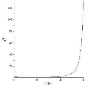
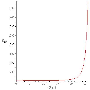
Figure 1: (left) The Brown-York energy for expansion branch of universe with D=4 and m=1 as a function of the t where t is the age of universe. In this plot, we choose $t_{s}=33Gyr$, $T_{M2}=100.$ and $l_{s}=0.1$. (right) In the right panel by taking the same values of the model parameters with $m=3$.

III The evolution of the Brown-York energy during the contraction branch in BIonic system

By now, we have shown that by closing M3-branes to each other, M2 dissolves in them and nonlinear gravities like Lovelock emerge. Now, we will show that by approaching branes to each other, the square energy of system become negative and system transits to tachyonic phase. To remove this state, Mp-branes compact, the sign of gravity changes and anti-gravity emerges which leads to getting away of branes from each other. In these conditions, temperature of system decreases, black hole disappears and the Brown-York energy vanishes. Using equation (30) we have:

$$l_{2}\rightarrow 0,l_{3}\rightarrow\infty,l_{2}^{\prime}\rightarrow\infty,l_{3}^{\prime}\rightarrow\infty\Rightarrow$$

$$l_{2}^{6}+l_{2}^{\prime 2}l_{2}^{2}-\lambda^{2}l_{3}^{\prime 2}<0$$

$$l_{3}^{6}+l_{3}^{\prime 2}l_{3}^{2}-\lambda^{2}l_{2}^{\prime 2}<0$$ (54)

This equation shows that by closing branes, the quantity under $\sqrt{}$ becomes negative and some tachyonic states are appeared. To solve this problem, branes are compactified and Mp-branes transit to Dp-branes. To show this, we use of the method in m18 and define ${\displaystyle<X^{10}>=\frac{r}{l_{p}^{3/2}}}$ where $l_{p}$ is the Planck length. We can write:

$$[X^{a},X^{b},X^{c}]=F^{abc}\quad[X^{a},X^{b}]=F^{ab}$$

$$F_{abc}=\partial_{a}A_{bc}-\partial_{b}A_{ca}+\partial_{c}A_{ab}\quad F_{ab}=\partial_{a}A_{b}-\partial_{b}A_{a}$$

$$\Sigma_{a,b,c=0}^{10}\langle F^{abc},F_{abc}\rangle = \Sigma_{a,b,c=0}^{10}\langle[X^{a},X^{b},X^{c}],[X_{a},X_{b},X_{c}]\rangle$$ (55)

$$= -\Sigma_{a,b,c,a^{\prime}b^{\prime}c^{\prime}=0}^{10}\varepsilon_{abcD}\varepsilon_{a^{\prime}b^{\prime}c^{\prime}G}^{D}X^{a}X^{b}X^{c}X_{a^{\prime}}X_{b^{\prime}}X_{c^{\prime}}$$

$$= -6\Sigma_{a,b,a^{\prime},b^{\prime}=0}^{9}\varepsilon_{ab10D}\varepsilon_{a^{\prime}b^{\prime}10}^{D}X^{a}X^{b}X^{10}X_{a^{\prime}}X_{b^{\prime}}X_{10}$$

$$- 6\Sigma_{a,b,c,a^{\prime},b^{\prime},c^{\prime}=0,\neq 10}^{9}\varepsilon_{abcD}\varepsilon_{a^{\prime}b^{\prime}c^{\prime}}^{D}X^{a}X^{b}X^{c}X_{a^{\prime}}X_{b^{\prime}}X_{c^{\prime}}$$

$$= -6\left(\frac{R^{2}}{l_{p}^{3}}\right)\Sigma_{a,b,a^{\prime},b^{\prime}=0}^{9}\varepsilon_{ab10D}\varepsilon_{a^{\prime}b^{\prime}10}^{D}X^{a}X^{b}X_{a^{\prime}}X_{b^{\prime}}$$

$$- 6\Sigma_{a,b,c,a^{\prime},b^{\prime},c^{\prime}=0,\neq 10}^{9}\varepsilon_{abcD}\varepsilon_{a^{\prime}b^{\prime}c^{\prime}}^{D}X^{a}X^{b}X^{c}X_{a^{\prime}}X_{b^{\prime}}X_{c^{\prime}}$$

$$= -6\left(\frac{R^{2}}{l_{p}^{3}}\right)\Sigma_{a,b=0}^{9}[X^{a},X^{b}]^{2}$$

$$- 6\Sigma_{a,b,c,a^{\prime},b^{\prime},c^{\prime}=0,\neq 10}^{9}\varepsilon_{abcD}\varepsilon_{a^{\prime}b^{\prime}c^{\prime}}^{D}X^{a}X^{b}X^{c}X_{a^{\prime}}X_{b^{\prime}}X_{c^{\prime}}$$

$$= -6\left(\frac{R^{2}}{l_{p}^{3}}\right)\Sigma_{a,b=0}^{9}F^{ab}F_{ab}+E_{Extra}$$

$$\partial_{a}X^{i}\partial_{a}X^{i}\sum(X^{j})^{2}=\Sigma_{a,i,j=0}^{10}\langle[X^{a},X^{i},X^{j}],[X_{a},X_{i},X_{j}]\rangle\Rightarrow$$

$$-6\left(\frac{R^{2}}{l_{p}^{3}}\right)\Sigma_{i,j=0}^{9}[X^{a},X^{j}][X_{a},X_{j}]=-6\left(\frac{R^{2}}{l_{p}^{3}}\right)\partial_{a}X^{i}\partial_{a}X^{i}\Rightarrow F(X)=\sum(X^{j})^{2}=1$$

$$\partial_{a}\partial_{b}X^{i}\partial_{a}\partial_{b}X^{i}=\Sigma_{a,b,i=0}^{10}\langle[X^{a},X^{b},X^{i}],[X_{a},X_{b},X_{i}]\rangle\Rightarrow$$

$$-6\left(\frac{R^{2}}{l_{p}^{3}}\right)\Sigma_{i,b=0}^{9}[X^{b},X^{i}][X_{b},X_{i}]=-6\left(\frac{R^{2}}{l_{p}^{3}}\right)\partial_{a}X^{i}\partial_{a}X^{i}$$

This equation shows that by compactification of branes, two form fields in eleven dimensional space-time converts to one form field and the sign of nonlinear terms in action change. Using equations (23) and (55), we can obtain the relation between noncompact and compact gravity :

$$A_{b}=e_{b}\quad F_{ab}=\partial_{a}e_{b}-\partial_{b}e_{a}\quad\kappa^{a}\vskip 3.0pt plus 1.0pt minus 1.0pt_{b}=\partial^{a}e_{b}$$

$$\Sigma_{\rho,\sigma,\mu,\nu=0}^{10}R^{\rho\sigma}_{\mu\nu}=\Sigma_{\rho,\sigma,\mu,\nu,\lambda=0}^{10}\langle F^{\rho\sigma}\vskip 3.0pt plus 1.0pt minus 1.0pt_{\lambda},F^{\lambda}\vskip 3.0pt plus 1.0pt minus 1.0pt_{\mu\nu}\rangle=\Sigma_{\rho,\sigma,\mu,\nu,\lambda=0}^{10}\langle[X^{\rho},X^{\sigma},X_{\lambda}],[X^{\lambda},X_{\mu},X_{\nu}]\rangle\Rightarrow$$

$$-6\left(\frac{R^{2}}{l_{p}^{3}}\right)\Sigma_{\rho,\sigma,\mu,\nu=0}^{9}[X^{\rho},X^{\sigma}][X_{\mu},X_{\nu}]=-6\left(\frac{R^{2}}{l_{p}^{3}}\right)\Sigma_{\rho,\sigma,\mu,\nu=0}^{9}F^{\rho\sigma}F_{\mu,\nu}=$$

$$-6(\frac{R^{2}}{l_{p}^{3}})\Sigma_{\rho,\sigma,\mu,\nu=0}^{9}\delta^{\rho\sigma}_{\rho^{\prime}\sigma^{\prime}}\delta_{\mu\nu}^{\mu^{\prime}\nu^{\prime}}\partial^{\rho^{\prime}}e^{\sigma^{\prime}}\partial_{\mu^{\prime}}e_{\nu^{\prime}}=-6\left(\frac{R^{2}}{l_{p}^{3}}\right)\Sigma_{\rho,\sigma,\mu,\nu=0}^{9}\delta^{\rho\sigma}_{\rho^{\prime}\sigma^{\prime}}\delta_{\mu\nu}^{\mu^{\prime}\nu^{\prime}}\kappa^{\rho^{\prime}\sigma^{\prime}}\kappa_{\mu^{\prime}\nu^{\prime}}$$

$$\Sigma_{\rho,\sigma,\mu,\nu=0}^{10}R=-6\left(\frac{R^{2}}{l_{p}^{3}}\right)\Sigma_{\rho,\sigma,\mu,\nu=0}^{9}\delta^{\mu\nu}_{\rho^{\prime}\sigma^{\prime}}\delta_{\mu\nu}^{\mu^{\prime}\nu^{\prime}}\kappa^{\rho^{\prime}\sigma^{\prime}}\kappa_{\mu^{\prime}\nu^{\prime}}$$ (56)

Above equation helps us to show that the sign of gravity changes:

$$\sum_{n=1}^{p}m_{g}^{2n}\delta^{\rho_{1}\sigma_{1}...\rho_{n}\sigma_{n}}_{\mu_{1}\nu_{1}...\mu_{n}\nu_{n}}R_{\rho_{1}\sigma_{1}}^{\mu_{1}\nu_{1}}...R_{\rho_{n}\sigma_{n}}^{\mu_{n}\nu_{n}}\Rightarrow-\sum_{n=1}^{p}m_{g}^{2n}\left(\frac{R^{2n}}{l_{p}^{3n}}\right)\delta^{\rho_{1}\sigma_{1}...\rho_{n}\sigma_{n}}_{\mu_{1}\nu_{1}...\mu_{n}\nu_{n}}\kappa^{\mu_{1}}_{\rho_{1}}\kappa^{\nu_{1}}_{\sigma_{1}}..\kappa^{\mu_{n}}_{\rho_{n}}\kappa^{\nu_{n}}_{\sigma_{n}}$$

$$\sum_{n=1}^{p}m_{g}^{2n}R^{n}\Rightarrow-\sum_{n=1}^{p}m_{g}^{2n}\left(\frac{R^{2n}}{l_{p}^{3n}}\right)\kappa^{\mu_{1}}_{\rho_{1}}\kappa^{\rho_{1}}_{\mu_{1}}..\kappa^{\mu_{n}}_{\rho_{n}}\kappa^{\rho_{n}}_{\mu_{n}}$$ (57)

Substituting relations in equation (57) in equation (29), we obtain:

$$S_{Mp} = -(T_{Mp})\int dt\int d^{p}\sigma\Biggl{[}\sqrt{-g}\Bigl{(}\sum_{n=1}^{p}\beta_{n}[-F(X)^{n}(1-m_{g}^{2})^{n}\left(\frac{R^{2n}}{l_{p}^{3n}}\right)\kappa^{\mu_{1}}_{\rho_{1}}\kappa^{\rho_{1}}_{\mu_{1}}..\kappa^{\mu_{n}}_{\rho_{n}}\kappa^{\rho_{n}}_{\mu_{n}}-$$ (58)

$$\sum_{n=1}^{p}m_{g}^{2n}\lambda^{2n}\left(\frac{R^{2n}}{l_{p}^{3n}}\right)\delta^{\rho_{1}\sigma_{1}...\rho_{n}\sigma_{n}}_{\mu_{1}\nu_{1}...\mu_{n}\nu_{n}}\kappa^{\mu_{1}}_{\rho_{1}}\kappa^{\nu_{1}}_{\sigma_{1}}..\kappa^{\mu_{n}}_{\rho_{n}}\kappa^{\nu_{n}}_{\sigma_{n}}]\Bigr{)}\Biggr{]}$$

This equation indicates that when Mp-branes are compactified, nonlinear gravity terms changes to other type of non-linear gravity terms with opposite sign. This can be a signature of anti-gravity. As due to the emergence of anti-gravity, M3-branes get away from each other and one M2-branes is produced between them. In our model, branes and anti-branes live on the M3-branes and thus, by closing towards each other, gravity changes to anti-gravity and prevents from approaching and disappearing branes. Using the relations in equation (55), we can show that the action (16) converts to following action:

$$S=-\frac{T_{Mp}}{2}\int d^{p+1}x\sum_{n=1}^{p}\beta_{n}\tilde{\chi}^{\mu_{0}}_{[\mu_{0}}\tilde{\chi}^{\mu_{1}}_{\mu_{1}}...\tilde{\chi}^{\mu_{n}}_{\mu_{n}]}$$

$$\tilde{\chi}\equiv STr\Bigg{(}-det(P_{ab}[E_{mn}E_{mi}(Q^{-1}+\delta)^{ij}E_{jn}+\lambda F_{ab}])det(Q^{i}_{j})\Bigg{)}^{1/2}~{}~{}$$

$$E_{mn}=G_{mn}+B_{mn},\qquad Q^{i}_{j}=\delta^{i}_{j}+i\lambda[X^{j},X^{k}]E_{kj}$$

$$G_{ab}=\eta_{ab}+\partial_{a}X^{i}\partial_{b}X^{i}$$ (59)

As can be seen from above equation, by compactifying M-theory, Mp-branes transit to Dp-branes. Similar to previous section, we assume that universes are placed on D3-branes which are connected by a D2-brane. To consider the evolution of branes, we assume the length of D2 between two D3 is $l_{2}$ and the length of each D3 be $l_{3}$ and obtain the relevant action for the system of D3-D2:

$$A^{ab}\rightarrow l_{3}\quad X^{i}\rightarrow l_{2}\quad\text{for D3-brane}$$

$$A^{ab}\rightarrow l_{2}\quad X^{i}\rightarrow l_{3}\quad\text{for D2-brane}$$

$$S_{tot}=S_{D3}+S_{D2}+S_{anti-D3}=$$

$$-2T_{D3}\int d^{6}\sigma\Sigma_{n=1}^{3}\beta_{n}(-l_{2}^{4}+l_{2}^{\prime 2}l_{2}^{2}+\lambda^{2}l_{3}^{\prime 2})^{\frac{n}{2}}$$

$$-2T_{D2}\int d^{3}\sigma\Sigma_{n=1}^{2}\beta_{n}(-l_{3}^{4}+l_{3}^{\prime 2}l_{3}^{2}+\lambda^{2}l_{2}^{\prime 2})^{\frac{n}{2}}\simeq$$

$$-2T_{D3}\int dtl_{3}^{3}\Sigma_{n=1}^{3}\beta_{n}(-l_{2}^{4}+l_{2}^{\prime 2}l_{2}^{2}+\lambda^{2}l_{3}^{\prime 2})^{\frac{n}{2}}$$

$$-2T_{D2}\int dtl_{2}^{2}\Sigma_{n=1}^{3}\beta_{n}(-l_{3}^{4}+l_{3}^{\prime 2}l_{3}^{2}+\lambda^{2}l_{2}^{\prime 2})^{\frac{n}{2}}$$ (60)

The equation of motion for this equation is:

$$-2T_{D3}\Sigma_{n=1}^{3}\beta_{n}[l_{3}^{3}(l_{2}^{\prime}l_{2}^{2})(-l_{2}^{4}+l_{2}^{\prime 2}l_{2}^{2}+\lambda^{2}l_{3}^{\prime 2})^{\frac{n}{2}-1}]^{\prime}$$

$$+2T_{D2}\Sigma_{n=1}^{2}\beta_{n}[(\lambda^{2}l_{2}^{2}l_{2}^{\prime}))(-l_{3}^{4}+l_{3}^{\prime 2}l_{3}^{2}+\lambda^{2}l_{2}^{\prime 2})^{\frac{n}{2}-1}]^{\prime}$$

$$+2T_{D3}\Sigma_{n=1}^{3}\beta_{n}[l_{3}^{3}(l_{2}^{\prime 2}l_{2}+2l_{2}^{3})(-l_{2}^{4}+l_{2}^{\prime 2}l_{2}^{2}+\lambda^{2}l_{3}^{\prime 2})^{\frac{n}{2}-1}]$$

$$-2T_{D2}\Sigma_{n=1}^{2}\beta_{n}[(l_{2}))(-l_{3}^{4}+l_{3}^{\prime 2}l_{3}^{2}+\lambda^{2}l_{2}^{\prime 2})^{\frac{n}{2}}]=0$$ (61)

$$-2T_{D2}\Sigma_{n=1}^{2}\beta_{n}[l_{2}^{2}(l_{3}^{\prime}l_{3}^{2})(-l_{3}^{4}+l_{3}^{\prime 2}l_{3}^{2}+\lambda^{2}l_{2}^{\prime 2})^{\frac{n}{2}-1}]^{\prime}$$

$$+2T_{D3}\Sigma_{n=1}^{3}\beta_{n}[(\lambda^{2}l_{3}^{3}l_{3}^{\prime}))(-l_{2}^{4}+l_{2}^{\prime 2}l_{2}^{2}+\lambda^{2}l_{3}^{\prime 2})^{\frac{n}{2}-1}]^{\prime}$$

$$+2T_{D2}\Sigma_{n=1}^{2}\beta_{n}[l_{2}^{2}(l_{3}^{\prime 2}l_{3}+2l_{3}^{3})(-l_{3}^{4}+l_{3}^{\prime 2}l_{3}^{2}+\lambda^{2}l_{2}^{\prime 2})^{\frac{n}{2}-1}]$$

$$-2T_{D3}\Sigma_{n=1}^{5}\beta_{n}[(3l_{3}^{2}))(-l_{2}^{4}+l_{2}^{\prime 2}l_{2}^{2}+\lambda^{2}l_{3}^{\prime 2})^{\frac{n}{2}}]=0$$ (62)

We can obtain the following approximate solutions for this equation:

$$l_{3}\simeq\sum_{n=1}^{3}\beta_{n}\frac{n}{\lambda^{n}T_{3}^{6n}}(\frac{t}{t_{s}}-1)^{-n}e^{-n\lambda\frac{t}{t_{s}}}$$

$$l_{2}\simeq\sum_{n=1}^{2}\beta_{n}\frac{1}{\lambda^{n}T_{2}^{3n}}(\frac{t}{t_{s}}-1)^{n}(1-e^{-n\lambda[\frac{t}{t_{s}}-1]})$$ (63)

This equation shows that at $t=t_{s}$, the separation distance ($l_{2}$) between two branes is zero and the size of D3 branes is infinite, while by passing time, branes get away from each other, $l_{2}\rightarrow\infty$ and $l_{3}\rightarrow 0$. This means that branes and anti-branes get away from each other and connect by a D2-brane. Similar to previous section, using equations (60 and 63), we derive the effective potential between branes and anti-branes:

$$t\rightarrow t_{s}\Rightarrow l_{3}\simeq l_{3}^{\prime}\simeq\frac{1}{l_{2}}\quad l_{2}^{\prime}\simeq\frac{1}{l_{2}}$$

$$V_{brane-antibrane}=2T_{M3}l_{2}^{-5}\Sigma_{n=1}^{5}\beta_{n}(l_{2}^{4}+1+\lambda^{2}l_{2}^{-2})^{\frac{n}{2}}$$

$$+2T_{M2}l_{2}^{2}\Sigma_{n=1}^{3}\beta_{n}(2l_{2}^{-4}+\lambda^{2}l_{2}^{-2})^{\frac{n}{2}}\simeq$$

$$b_{1}l_{2}+b_{2}l_{2}^{-3}+b_{3}l_{2}^{-5}+b_{4}l_{2}^{-6}+....$$ (64)

where $b_{i}$’s are some coefficients which depend on the tension of branes and $\lambda$. This equation shows that by compacting branes, order of $l_{2}^{-1}$ increases. This is because that near the colliding point $l_{2}\rightarrow 0$, the repulsive potential is very large and shrinks to zero at infinity. Now, we obtain temperature of system by using the equations (43 and 64):

$$T=\frac{\gamma}{\pi}(\frac{w^{\prime}}{w})^{1/2}\sim\frac{\gamma}{\pi}(\frac{V^{\prime}}{V})^{1/2}\sim$$

$$\frac{\gamma}{\pi}\left(\frac{b_{1}+b_{2}l_{2}^{-4}+b_{3}l_{2}^{-6}+b_{4}l_{2}^{-7}}{b_{1}l_{2}+b_{2}l_{2}^{-3}+b_{3}l_{2}^{-5}+b_{4}l_{2}^{-6}}\right)^{1/2}$$ (65)

Substituting equation (44) in above equation , we can obtain the size of M2 in terms of the temperature:

$$l_{2}\simeq T^{2}[\frac{6}{k\sqrt{3}}-\bar{T}^{2}]^{2}$$ (66)

Similar to previous section, by definition of $k=\frac{\sqrt{3}}{6}$, temperature of colliding point and critical temperature become equal ($T_{\text{colliding point}}=T_{c}$). Substituting equations (63,41,42,43,44and 45)in equation (III) for m=1 and D=4 and in the limit $r\sim z\sim l_{2}\rightarrow 0$, we obtain:

$$E_{BY}\sim[\sum_{n=1}^{2}\beta_{n}\frac{1}{\lambda^{n}T_{2}^{3n}}(\frac{t}{t_{s}}-1)^{n}(1-e^{-n\lambda[\frac{t}{t_{s}}-1]})]+\Big{(}\frac{l_{2,0}^{4}}{[\sum_{n=1}^{2}\beta_{n}\frac{1}{\lambda^{n}T_{2}^{3n}}(\frac{t}{t_{s}}-1)^{n}(1-e^{-n\lambda[\frac{t}{t_{s}}-1]})]^{3}}\times$$

$$[\frac{1}{1+\frac{\beta^{2}}{[\sum_{n=1}^{2}\beta_{n}\frac{1}{\lambda^{n}T_{2}^{3n}}(\frac{t}{t_{s}}-1)^{n}(1-e^{-n\lambda[\frac{t}{t_{s}}-1]})]^{4}}}+[1+\frac{l_{2,0}^{4}}{[\sum_{n=1}^{2}\beta_{n}\frac{1}{\lambda^{n}T_{2}^{3n}}(\frac{t}{t_{s}}-1)^{n}(1-e^{-n\lambda[\frac{t}{t_{s}}-1]})]^{4}}[1-$$

$$(\frac{3\sqrt{3}-\bar{T}^{4}\sqrt{1+\frac{k^{2}}{[\sum_{n=1}^{2}\beta_{n}\frac{1}{\lambda^{n}T_{2}^{3n}}(\frac{t}{t_{s}}-1)^{n}(1-e^{-n\lambda[\frac{t}{t_{s}}-1]})]^{4}}}-\frac{\sqrt{3}}{6}\bar{T}^{8}(1+\frac{k^{2}}{[\sum_{n=1}^{2}\beta_{n}\frac{1}{\lambda^{n}T_{2}^{3n}}(\frac{t}{t_{s}}-1)^{n}(1-e^{-n\lambda[\frac{t}{t_{s}}-1]})]^{4}})}{2\bar{T}^{4}\sqrt{1+\frac{k^{2}}{[\sum_{n=1}^{2}\beta_{n}\frac{1}{\lambda^{n}T_{2}^{3n}}(\frac{t}{t_{s}}-1)^{n}(1-e^{-n\lambda[\frac{t}{t_{s}}-1]})]^{4}}}})^{2}]]^{-1}\times$$

$$[1-\frac{1}{1+\frac{\beta^{2}}{[\sum_{n=1}^{2}\beta_{n}\frac{1}{\lambda^{n}T_{2}^{3n}}(\frac{t}{t_{s}}-1)^{n}(1-e^{-n\lambda[\frac{t}{t_{s}}-1]})]^{4}}}]]^{-1/2}[1+\frac{l_{2,0}^{4}}{[\sum_{n=1}^{2}\beta_{n}\frac{1}{\lambda^{n}T_{2}^{3n}}(\frac{t}{t_{s}}-1)^{n}(1-e^{-n\lambda[\frac{t}{t_{s}}-1]})]^{4}}\times$$

$$[(\frac{3\sqrt{3}-\bar{T}^{4}\sqrt{1+\frac{k^{2}}{[\sum_{n=1}^{2}\beta_{n}\frac{1}{\lambda^{n}T_{2}^{3n}}(\frac{t}{t_{s}}-1)^{n}(1-e^{-n\lambda[\frac{t}{t_{s}}-1]})]^{4}}}-\frac{\sqrt{3}}{6}\bar{T}^{8}(1+\frac{k^{2}}{[\sum_{n=1}^{2}\beta_{n}\frac{1}{\lambda^{n}T_{2}^{3n}}(\frac{t}{t_{s}}-1)^{n}(1-e^{-n\lambda[\frac{t}{t_{s}}-1]})]^{4}})}{2\bar{T}^{4}\sqrt{1+\frac{k^{2}}{[\sum_{n=1}^{2}\beta_{n}\frac{1}{\lambda^{n}T_{2}^{3n}}(\frac{t}{t_{s}}-1)^{n}(1-e^{-n\lambda[\frac{t}{t_{s}}-1]})]^{4}}}})^{2}]]^{-1/2}\Big{)}$$

This equation shows that by passing time and increasing the separation distance between two branes ($l_{2}$), the Brown-York energy decreases and shrinks to zero at large values of time (See Figure 2(Left).). This is because that by getting away of M3-branes, the nonlinear gravity like the Lovelock gravity disappears and temperature and also the gravitational energy of system decreases. Using equation (III), we can obtain the Brown-York energy for mth order of Lovelock gravity for a system with D=3m+1

$$\overline{E}_{BY}=r^{m}[D_{0}(\frac{E_{BY}}{r})^{2m-1}+...+D_{s}(\frac{E_{BY}}{r})^{2m-2s-1}(1-D^{1/2}\bar{H}^{-1/2}f)^{s}+...D_{m-1}(\frac{E_{BY}}{r})^{m-1}(1-\sqrt{D^{1/2}\bar{H}^{-1/2}f})]$$

For m=1, above equation reduces to equation (III). This equation shows that by increasing number of dimensions the effect of Lovelock gravity increases and consequently, more changes can be observed in energy of system (See Figure2(Right)). This is because that by increasing the number of dimensions, there exists many channels for flowing energy from extra dimensions and other universes to our own universe which leads to the emergence of higher order terms in gravity.

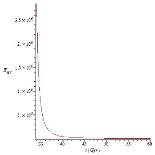
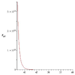
Figure 2: (left) The Brown-York energy for contraction branch of universe with D=4 and m=1 as a function of the t where t is the age of universe. In this plot, we choose $t_{s}=33Gyr$, $T_{M2}=100.$ and $l_{s}=0.1$. (right) In the right panel by taking the same values of the model parameters with $m=3$.

IV Summary and Discussion

In this research, we have used the idea of s5 for measuring the gravitational energy in Lovelock gravity for considering the evolution of BIonic system. In our model, first M0-branes join each other and form a system of one M3, one anti-M3 and an M2-brane. Brane lives on an M3, anti-brane is placed on an anti-M3 and M2 connects them. M2 plays the role of wormhole between branes and is the main cause of gravitational energy in BIonic system. By dissolving M2 in M3-branes, Lovelock gravity is produced and M3 expands. By closing branes to each other, wormhole becomes thermal and transits to black hole. During this epoch, the Brown-York increases and shrinks to large values. By approaching branes, the square energy of M2-M3 system becomes negative and some tachyonic states are created. To remove these states, M2 and M3-branes compact, gravity converts to anti-gravity and branes get away from each other. We have calculated the potential between branes and anti-branes and find that it is in agreement with previous predictions. This means that usual potential between branes may be produced by dissolving M2-branes in M3-branes which branes live on it. On the other hand, by closing branes and disappearing M2, Lovelock gravity emerges. Thus, the Lovelock gravity may be the main cause of the wormhole and gravitational energy between branes and anti-branes. During this era, the Brown-York decreases and shrinks to zero.

References

(1)
J. D. Brown and J. W. York, Phys.Rev. D47 (1993) 1407–1419, arXiv:gr-qc/9209012 [gr-qc].
(2)
N. Dadhich arXiv:gr-qc/9704068 [gr-qc].
(3)
N. Dadhich, Curr.Sci. 76 (1999)831, arXiv:gr-qc/9705037 [gr-qc].
(4)
S. Bose and N. Dadhich, Phys.Rev. D60
(1999) 064010, arXiv:gr-qc/9906063 [gr-qc].
(5)
S. Bose and T. Z. Naing, Phys.Rev. D60 (1999) 104027.
(15)
Claudia de Rham, Andrew J. Tolley, Shuang-Yong Zhou,
arXiv:1512.06838.
Claudia de Rham, Gregory Gabadadze, Andrew J.
Tolley, Phys.Rev.Lett.106:231101,2011.
L. Heisenberg, R. Kimura, K. Yamamoto, Phys. Rev. D 89 103008 (2014).
M. Cruz, E. Rojas, Class. Quantum Grav. 30, 115012 (2013).
A.Sepehri, submitted to journal, in proceeding.
(16)
R. C. Myers, JHEP 12, 022 (1999), hep-th/9910053.
N. R. Constable, R. C. Myers, O. Tafjord, JHEP 0106, 023 (2001).
A. A. Tseytlin, hep-th/9908105 (1999).
(17)
Chong-Sun Chu, Douglas J Smith, JHEP 0904, 097 (2009).
(18)
B. Sathiapalan, Nilanjan Sircar, JHEP 0808, 019 (2008).
(19)
N. R. Constable, Robert C. Myers, Oyvind Tafjord, Phys. Rev. D 61,
106009 (2000).
(20)
J. Kluson, JHEP 0011, 016 (2000).
(21) J. Bagger and N. Lambert, Gauge Symmetry and Supersymmetry of Multiple M2-Branes,
Phys. Rev. D 77, 065008 (2008) [arXiv:0711.0955 [hep-th]].
(22) A. Gustavsson, Algebraic structures on parallel M2-branes, arXiv:0709.1260 [hep-th].
(30)
P. Bicudo, M. Cardoso, O. Oliveira, Phys.Rev.D77:091504,2008.
Yannis Burnier, Olaf Kaczmarek, Alexander Rothkopf, Phys. Rev.
Lett. 114, 082001 (2015).
(31)
Gianluca Grignani, Troels Harmark, Andrea Marini, Niels A. Obers, Marta Orselli, JHEP
1106:058,2011.
T. Harmark, JHEP 07 (2000) 043,
arXiv:hep-th/0006023.
Gianluca Grignani, Troels Harmark, Andrea
Marini, Niels A. Obers, Marta Orselli,
Nucl.Phys.B851:462-480,2011.