Photon merging and splitting in electromagnetic field inhomogeneities

Abstract

We investigate photon merging and splitting processes in inhomogeneous, slowly varying electromagnetic fields. Our study is based on the three-photon polarization tensor following from the Heisenberg-Euler effective action. We put special emphasis on deviations from the well-known constant field results, also revisiting the selection rules for these processes. In the context of high-intensity laser facilities, we analytically determine compact expressions for the number of merged/split photons as obtained in the focal spots of intense laser beams. For the parameter range of a typical petawatt class laser system as pump and a terawatt class laser as probe, we provide estimates for the numbers of signal photons attainable in an actual experiment. The combination of frequency upshifting, polarization dependence and scattering off the inhomogeneities renders photon merging an ideal signature for the experimental exploration of nonlinear quantum vacuum properties.

I Introduction

The vacuum of quantum electrodynamics (QED) acquires properties akin to those of ordinary polarizable matter when subjected to strong electromagnetic fields Euler:1935zz ; Heisenberg:1935qt ; Weisskopf . These fields can couple to electron-positron fluctuations inducing nonlinear interactions (for reviews, see Dittrich:1985yb ; Dittrich:2000zu ; Marklund:2008gj ; Dunne:2008kc ; Heinzl:2008an ; DiPiazza:2011tq ; Dunne:2012vv ; Battesti:2012hf ; King:2015tba ). The spatial and temporal scale associated to these electron-positron fluctuations is set by the Compton wavelength $\lambda_{C}=1/m\approx 3.86\times 10^{-13}{\rm m}$ and the Compton time $\tau_{C}=1/m\approx 1.29\times 10^{-21}{\rm s}$ of the electron respectively, where $m\approx 511{\rm keV}$ denotes the electron mass. At leading order in the field strengths prominent signatures of quantum vacuum nonlinearities such as vacuum magnetic birefringence Toll:1952 ; Baier ; BialynickaBirula:1970vy and direct light-by-light scattering Euler:1935zz ; Karplus:1950zz are mediated by an effective four-photon interaction.

The resulting nonlinear interactions among laboratory electromagnetic fields are suppressed by powers of the field strength ratio $\mathcal{E}/\mathcal{E}_{\rm cr}$, with $\cal E$ denoting the electric/magnetic field amplitude and $\mathcal{E}_{\rm cr}=m^{2}/e\approx 1.3\cdot 10^{18}{\rm V/m}\approx 4\cdot 10^{9}{\rm T}$ the critical field strength. Hence, experimental verifications Akhmadaliev:1998zz ; Akhmadaliev:2001ik have so far been limited to high-energy experiments probing vacuum nonlinearities in the strong Coulomb fields in the vicinity of highly charged ions (Delbrück-scattering Delbrueck:1933 ; Bethe:1952yya and photon splitting Adler:1971wn ; Lee:1998hu ). Vacuum nonlinearities in macroscopic electromagnetic fields have not been directly verified so far. Direct searches of vacuum magnetic birefringence in macroscopic magnetic fields Cantatore:2008zz ; Berceau:2011zz for instance, have already demonstrated that a combination of both high field strength as well as a high signal detection sensitivity will eventually be needed for a first discovery, see Zavattini:2016sqz for a recent proposal.

On the other hand, recent technological advances in the development of high-intensity lasers have begun to access new extreme-field territory. The perspective to directly probe quantum vacuum nonlinearities in all-optical pump-probe type set-ups is most promising: one high-intensity laser (“pump”) generates a strong electromagnetic field pulse polarizing the quantum vacuum in its focus, which is then probed by a second high-intensity laser. A prominent example is the fundamental physics program within the HIBEF project HIBEF , which plans to combine a near-infrared petawatt (PW) laser as pump and the European XFEL as probe laser aiming to detect vacuum birefringence Heinzl:2006xc ; Karbstein:2015xra ; Schlenvoigt:2016 , see also DiPiazza:2006pr ; Dinu:2013gaa for related work. While the advantage of using ultra-intense lasers is obvious from the accessible field strengths, important progress also has been made on the detection side in the form of high-purity x-ray polarimetry Uschmann:2014 . Further attractive theoretical proposals have focused on optical signatures of quantum vacuum nonlinearities based on interference effects King:2013am ; Tommasini:2010fb ; Hatsagortsyan:2011 , photon-photon scattering in the form of laser-pulse collisions Lundstrom:2005za ; Lundin:2006wu ; King:2012aw and quantum reflection Gies:2013yxa .

In some of these studies, a new ingredient in addition to extreme fields and high detection efficiencies has been identified: as laser pulses feature an intrinsic spatio-temporal structure, these spacetime inhomogeneities allow for a richer variety of quantum vacuum signatures that remains invisible in the idealized theoretical limit of constant homogeneous fields.

To this end, recently a representation of the one-loop photon polarization tensor $\Pi^{\mu\nu}(k,k^{\prime})$ (photon two-point function) in the limit of low energies and momenta and for slowly varying but otherwise arbitrary electromagnetic field inhomogeneities has been derived Karbstein:2015cpa . Note that essentially all macroscopic electromagnetic fields attainable in the laboratory fall into this category, as they vary on scales much larger than the Compton wavelength and time of the electron. This result facilitates a straightforward investigation of photon propagation effects in high-intensity laser fields. Whereas constant electromagnetic fields only affect a probe photon’s polarization properties, inhomogeneous fields may additionally alter its frequency and wave vector, which can be employed to physically separate the (tiny) amount of photons carrying the signature from a large background consisting of probe photons unaffected by quantum vacuum nonlinearities; inhomogeneities thus become the key ingredient for some phenomena such as quantum reflection Gies:2013yxa .

Besides propagation effects, photons in strong electromagnetic fields can also experience splitting BialynickaBirula:1970vy ; Adler:1971wn ; Adler:1970gg ; Papanyan:1971cv ; Papanyan:1973xa ; Stoneham:1979 ; Baier:1986cv ; Baier:1996bq ; Adler:1996cja ; DiPiazza:2007yx and merging Yakovlev:1966 ; DiPiazza:2007cu ; Gies:2014jia . Photon splitting describes processes where a single photon splits into two or more outgoing photons under the influence of an external electromagnetic field. Photon merging can be viewed as the inverse process: two or more photons merge under the influence of the external field, yielding a single outgoing photon. The first detailed investigation of photon splitting has been performed by Adler in 1971 Adler:1971wn , who considered this process in a constant, purely magnetic background field.

In this work we aim at adopting the strategy devised in Karbstein:2014fva ; Karbstein:2015cpa ; Karbstein:2015xra to study photon splitting and merging in the strong, inhomogeneous electromagnetic fields attainable with high-intensity laser experiments. For this, we start in Sect. II by deriving the “three-photon polarization tensor” $\Pi^{\mu\nu\rho}(k,k^{\prime},k^{\prime\prime})$ to one-loop order in the limit of low energies and momenta and for weakly-varying but otherwise arbitrary electromagnetic field inhomogeneities. This quantity describes the effective interaction between three photon fields facilitated by vacuum fluctuations in the presence of external electromagnetic fields. It accounts for couplings to the external field to all orders. We furthermore detail on how to determine the amplitudes and numbers of signal photons for the splitting and merging processes. In Sect. III, we analyze the polarization properties and selection rules for photon splitting and merging. More specifically, we focus on the special class of field inhomogeneities characterized by unidirectional orthogonal electric and magnetic fields of equal strength, but featuring arbitrary field amplitude profiles. In Sect. IV, we consider a specific field amplitude profile and compare the magnitudes of the numbers of photons experiencing photon splitting and merging in this field inhomogeneity. Finally, we provide estimates for the number of accessible signal photons from the photon merging process for realistic laser parameters. We finish with a conclusion in Sect. V.

II The three-photon polarization tensor in an electromagnetic field inhomogeneity

The goal of this article is to study photon splitting and merging in an all-optical experiment, where both pump and probe fields are provided by lasers. We consider a macroscopic “probe” photon field $a_{\rho}(q)$ traversing an electromagnetic “pump“ field configuration described by the field-strength profile $F^{\mu\nu}(x)$. The nonlinear interactions between the pump and probe fields may induce outgoing signal photons via the effective interactions of the probe and pump fields. Each signal photon is characterized by its four-momentum $k^{\mu}$ and polarization four-vector $\epsilon_{\sigma}^{*(p)}(k)$, where $p$ labels the two transverse photon polarizations. For photon splitting we study the process linear in the probe photon field giving rise to two outgoing signal photons. Conversely, for photon merging we consider the process quadratic in the probe photon field resulting in a single signal photon. More specifically, the amplitude $\mathcal{M}_{\rm Split}^{p\rightarrow p^{\prime}p^{\prime\prime}}(k^{\prime},k^{\prime\prime})$ for photons from a macroscopic probe photon field $a_{\rho}^{(p)}(q)$, with momentum $q^{\mu}$ and polarization vector $\epsilon_{\rho}^{(p)}(q)$, to split into two real photons with momenta ${k^{\prime}}^{\mu}=(|\mathbf{k}^{\prime}|,\mathbf{k}^{\prime})$ and ${k^{\prime\prime}}^{\mu}=(|\mathbf{k}^{\prime\prime}|,\mathbf{k}^{\prime\prime})$, and polarization vectors $\epsilon_{\sigma}^{*(p^{\prime})}(k^{\prime})$ and $\epsilon_{\eta}^{*(p^{\prime\prime})}(k^{\prime\prime})$ respectively, is given by

$$\mathcal{M}_{\rm Split}^{p\rightarrow p^{\prime}p^{\prime\prime}}(k^{\prime},k^{\prime\prime})=\frac{\epsilon_{\sigma}^{*(p^{\prime})}(k^{\prime})}{\sqrt{2|\mathbf{k}^{\prime}|}}\,\frac{\epsilon_{\eta}^{*(p^{\prime\prime})}(k^{\prime\prime})}{\sqrt{2|\mathbf{k}^{\prime\prime}|}}\int_{q}\Pi^{\rho\sigma\eta}(-q,k^{\prime},k^{\prime\prime}|F)a_{\rho}^{(p)}(q).$$ (1)

Here, $\Pi^{\rho\sigma\eta}(-q,k^{\prime},k^{\prime\prime}|F)$ denotes the three-photon polarization tensor (three-point proper vertex) in an external electromagnetic field inhomogeneity $F^{\mu\nu}(x)$, and the indices $p,p^{\prime},p^{\prime\prime}$ label the polarizations of the incident probe photon beam and the signal photons to be specified later. We use “all-outgoing” sign conventions for the momentum arguments of $\Pi^{\rho\sigma\eta}$. At one loop-order, the three-photon polarization tensor quantifies the effective coupling of three photon fields mediated by an electron-positron loop. At this stage, $\Pi^{\rho\sigma\eta}$ accounts for the coupling to the field inhomogeneity $F^{\mu\nu}(x)$ to all orders, see Fig. 1. Throughout the paper we work in Heaviside-Lorentz units, setting $\hbar=c=1$. Spatio-temporal four vectors are denoted by italic letters, $x^{\mu}=(t,{\rm x},{\rm y},{\rm z})$, for the spatial components we use roman letters. Our metric is $g^{\mu\nu}=(-,+,+,+)$, such that $kx\equiv k_{\mu}x^{\mu}=(-k^{0}t+\mathbf{k}\cdot\mathbf{x})$. We employ the short-hand notation $\int_{q}\equiv\int\frac{{\rm d}^{4}q}{(2\pi)^{4}}$ for momentum integrations, and $\int_{x}\equiv\int{\rm d}^{4}x$ for space-time integrations.

In analogy to Eq. (1), the amplitude $\mathcal{M}^{p^{\prime}p^{\prime\prime}\rightarrow p}_{\rm Merg}(k)$ for merging photons from the probe field to yield a single outgoing photon with momentum $k^{\mu}=(|\mathbf{k}|,\mathbf{k})$ and polarization vector $\epsilon_{\rho}^{*(p)}(k)$ reads

$$\mathcal{M}^{p^{\prime}p^{\prime\prime}\rightarrow p}_{\rm Merg}(k)=\frac{\epsilon_{\rho}^{*(p)}(k)}{\sqrt{2|\mathbf{k}|}}\,\int_{q^{\prime}}\int_{q^{\prime\prime}}\Pi^{\rho\sigma\eta}(k,-q^{\prime},-q^{\prime\prime}|F)a^{\prime}_{\sigma}{}^{(p^{\prime})}(q^{\prime})a^{\prime\prime}_{\eta}{}^{(p^{\prime\prime})}(q^{\prime\prime}).$$ (2)

Here we accounted for the most generic situation, where the merged photons are originating from two distinct probe photon fields $a^{\prime}_{\sigma}{}^{(p^{\prime})}(q^{\prime})$ and $a^{\prime\prime}_{\eta}{}^{(p^{\prime\prime})}(q^{\prime\prime})$ with polarizations $p^{\prime}$ and $p^{\prime\prime}$, respectively.

Figure 1: Feynman diagrams of the three-photon interactions considered in this work. (a) Photon Splitting: An incoming photon with momentum $k^{\mu}$ and polarization four-vector $\epsilon_{\rho}^{(p)}(k)$ splits, under the assistance of the external field inhomogeneity $F^{\mu\nu}(x)$, into two photons with $\bigl{\{}{k^{\prime}}^{\mu}$, $\epsilon_{\sigma}^{*(p^{\prime})}(k^{\prime})\bigr{\}}$ and $\bigl{\{}{k^{\prime\prime}}^{\mu}$, $\epsilon_{\eta}^{*(p^{\prime\prime})}(k^{\prime\prime})\bigr{\}}$. (b) Photon Merging: Two incoming photons with $\bigl{\{}{k^{\prime}}^{\mu}$, $\epsilon_{\sigma}^{(p^{\prime})}(k^{\prime})\bigl{\}}$ and $\bigl{\{}{k^{\prime\prime}}^{\mu}$, $\epsilon_{\eta}^{(p^{\prime\prime})}(k^{\prime\prime})\bigl{\}}$ merge to yield a single outgoing photon with $\bigl{\{}k^{\mu}$, $\epsilon_{\rho}^{*(p)}(k)\bigl{\}}$. The coupling of the probe photons and the external field inhomogeneity $F^{\mu\nu}(x)$ to the electron-positron loop is encoded in the three-photon polarization tensor $\Pi^{\rho\sigma\eta}$.

The physical information about the splitting and merging processes in Eqs. (1) and (2) is encoded in the three-photon polarization tensor. At present, no exact analytical results for the three-photon polarization tensor for arbitrary momentum transfers and background field inhomogeneities are known. At one-loop order and for generic momentum transfers, exact results for two classes of background field configurations are available. The first class comprises uniform electromagnetic fields: Papanyan and Ritus Papanyan:1971cv ; Papanyan:1973xa derived a parameter integral representation of the three-photon polarization tensor in “constant-crossed” fields, i.e. for orthogonal constant electric and magnetic fields of equal amplitude $|\mathbf{E}|=|\mathbf{B}|=:\mathcal{E}$. For this setting, the field invariants $\mathcal{F}=\frac{1}{4}F_{\mu\nu}F^{\mu\nu}=\frac{1}{2}(\mathbf{B}^{2}-\mathbf{E}^{2})$ and $\mathcal{G}=\frac{1}{4}F_{\mu\nu}{}^{*}F^{\mu\nu}=-\mathbf{E}\cdot\mathbf{B}$ vanish; ${}^{*}F^{\mu\nu}=\frac{1}{2}\epsilon^{\mu\nu\alpha\beta}F_{\alpha\beta}$ denotes the dual field strength tensor. Later, splitting amplitudes valid for arbitrary photon energies have been derived in constant, but generically oriented electromagnetic fields Baier:1986cv . Energy-momentum conservation in constant fields implies that all three photons propagate collinearly. As a consequence, an expansion of the amplitude in the background field strength starts with terms $\propto\left(\frac{e\mathcal{E}}{m^{2}}\right)^{3}$, i.e., arising from a hexagon diagram in accordance with the Adler theorem Adler:1971wn . This will also become manifest in our results below.

The second class of background field configurations encompasses plane-wave backgrounds with vector potential $A_{\mu}(\kappa x)$, where $\kappa^{\mu}=(|\boldsymbol{\kappa}|,\boldsymbol{\kappa})$ denotes the four-momentum of the plane wave. Photon splitting amplitudes for arbitrary photon energies in this class of background fields have been derived in DiPiazza:2007yx . Recall that photon splitting amplitudes amount to on-shell matrix elements of the three-photon photon polarization tensor. In this configuration, the probe photons can exchange energy and momentum with the background field, and an expansion in the background field strength hence generically starts with terms $\propto\left(\frac{e\mathcal{E}}{m^{2}}\right)$, corresponding to box diagrams. For small angles between the photon momenta, splitting amplitudes have also been calculated in Coulomb fields Lee:1998hu .

A study of photon splitting and merging in generic background field inhomogeneities may eventually require dedicated numerical efforts, see, e.g., worldline . However, in the present work we confine ourselves to field inhomogeneities whose spatial and temporal variation, $w$ and $\tau$, are large compared to the spatial and temporal Compton scale of the electron-positron loop, i.e., $w\gg\lambda_{C}$ and $\tau\gg\tau_{C}$. These slowly varying fields mark the regime of the locally constant field approximation (LCFA). As a matter of fact, practically all current and proposed all-optical probes of QED vacuum nonlinearities in macroscopic fields fall into this category.

The LCFA corresponds to treating the microscopic quantum fluctuations as propagating in a constant field at each point in spacetime. This culminates in the effective Heisenberg-Euler Lagrangian $\mathcal{L}(x|F)$ which is a local function of spacetime. On the macroscopic level, this Lagrangian can now be applied locally. In the present work, we use it to calculate the three-photon polarization tensor for manifestly inhomogeneous background field profiles following the strategy of Karbstein:2015cpa . For strictly constant background fields, an analogous idea has originally been adopted by Adler Adler:1971wn and Bialynicka-Birula BialynickaBirula:1970vy in the 1970s to study photon splitting. Still, it is important to realize that the same line or reasoning also applies to slowly varying fields with parametrically suppressed errors which are quantified below. The photon polarization tensor derived in this way is manifestly restricted to low four-momentum transfers; i.e., also the probe photons have to be slowly varying. Let us emphasize that this procedure manifestly preserves gauge invariance and therefore retains complete information about the polarization properties of the involved photons for any given slowly varying background field inhomogeneity.

Our starting point is the one-loop effective action $\mathcal{S}_{\rm int}(F,f)=\int_{x}\mathcal{L}(x|F+f)$, mediating effective interactions between probe photon fields $a_{\mu}(x)$, with field strength tensor $f^{\mu\nu}(x)$, in a background field inhomogeneity with field strength tensor $F^{\mu\nu}(x)$. It is obtained from the Heisenberg-Euler Lagrangian for constant fields, which only depends on the field strength tensor $F^{\mu\nu}$, by substituting $F^{\mu\nu}\to F^{\mu\nu}(x)+f^{\mu\nu}(x)$, cf. Karbstein:2015cpa . Correspondingly, the effective interactions among the probe photons can be seen as generated by derivatives of the Heisenberg-Euler Lagrangian. An expansion in terms of probe photons reads

$$\mathcal{S}_{\rm int}=\mathcal{S}^{(1)}_{\rm int}+\mathcal{S}^{(2)}_{\rm int}+\mathcal{S}^{(3)}_{\rm int}+...=\int_{x}\frac{\partial\mathcal{L}}{\partial F^{\mu\nu}}f^{\mu\nu}\,+\frac{1}{2!}\int_{x}\frac{\partial^{2}\mathcal{L}}{\partial F^{\mu\nu}\partial F^{\alpha\beta}}f^{\mu\nu}f^{\alpha\beta}\,+\frac{1}{3!}\int_{x}\frac{\partial^{3}\mathcal{L}}{\partial F^{\mu\nu}\partial F^{\alpha\beta}\partial F^{\gamma\delta}}f^{\mu\nu}f^{\alpha\beta}f^{\gamma\delta}\,+...\quad,$$ (3)

where $S_{\rm int}^{(l)}$ contains the effective interaction between $l$ photons. To keep the notation compact, we have omitted the spacetime arguments of the fields. As a consequence of Furry’s theorem, only an even number of contractions of $F^{\mu\nu}(x)$ and $f^{\mu\nu}(x)$ may constitute building blocks of the Lagrangian. On the level of the action, the LCFA neglects derivatives of the field strength tensors which are generic constituents of the exact effective Lagrangian. Derivatives of the fields in position space translate to multiplications of the fields in momentum space with their typical momentum $v$. As the action is dimensionless, the LCFA therefore inherently neglects contributions of $\mathcal{O}\bigl{(}\frac{v^{2}}{m^{2}}\bigr{)}$, with the electron mass $m$ as the only dimensionful scale in QED.

The lowest order interaction term $\mathcal{S}^{(1)}_{\rm int}$ of the expansion (3) describes vacuum emission processes Karbstein:2014fva . The second order term $\mathcal{S}^{(2)}_{\rm int}$ entails propagation effects Karbstein:2015cpa , such as vacuum birefringence Karbstein:2015xra and quantum reflection Gies:2013yxa . Finally, the third order term $\mathcal{S}^{(3)}_{\rm int}$ encodes three-photon interactions such as splitting and merging to be considered here. The three-photon polarization tensor in momentum space is now easily inferred from $\mathcal{S}^{(3)}_{\rm int}$. Employing the momentum space representation of the probe photons, $a^{\mu}(x)=\int_{k}{\rm e}^{ikx}a^{\mu}(k)$, we substitute $f^{\mu\nu}(x)=i\int_{k}{\rm e}^{ikx}\bigl{[}k^{\mu}g^{\nu\sigma}-k^{\nu}g^{\mu\sigma}\bigr{]}a_{\sigma}(k)$ into $\mathcal{S}_{\rm int}^{(3)}$ and obtain

$$\mathcal{S}_{\rm int}^{(3)}=-\frac{1}{3!}\int_{k}\int_{k^{\prime}}\int_{k^{\prime\prime}}a_{\rho}(k)a_{\sigma}(k^{\prime})a_{\eta}(k^{\prime\prime})\Pi^{\rho\sigma\eta}(k,k^{\prime},k^{\prime\prime}),$$ (4)

where the three-photon polarization tensor has been defined as

$$\Pi^{\rho\sigma\eta}(k,k^{\prime},k^{\prime\prime}):=i(k^{\mu}g^{\nu\rho}-k^{\nu}g^{\mu\rho})(k^{\prime}{}^{\alpha}g^{\beta\sigma}-k^{\prime}{}^{\beta}g^{\alpha\sigma})(k^{\prime\prime}{}^{\gamma}g^{\delta\eta}-k^{\prime\prime}{}^{\delta}g^{\gamma\eta})\int_{x}{\rm e}^{i(k+k^{\prime}+k^{\prime\prime})x}\frac{\partial^{3}\mathcal{L}}{\partial F^{\mu\nu}\partial F^{\alpha\beta}\partial F^{\gamma\delta}}(x).$$ (5)

The tensorial structure guarantees that the Ward-identity, ensuring gauge invariance, is fulfilled: $k_{\rho}\Pi^{\rho\sigma\eta}(k,k^{\prime},k^{\prime\prime})=k^{\prime}_{\sigma}\Pi^{\rho\sigma\eta}(k,k^{\prime},k^{\prime\prime})=k^{\prime\prime}_{\eta}\Pi^{\rho\sigma\eta}(k,k^{\prime},k^{\prime\prime})=0$. This three-photon polarization tensor neglects contributions of order $v^{3}\mathcal{O}\bigl{(}\frac{v^{2}}{m^{2}}\bigr{)}$.

For explicit calculations it is useful to rewrite the derivatives of the Lagrangian with respect to $F^{\mu\nu}$ in terms of the invariants $\mathcal{F}$ and $\mathcal{G}$. Then, the third derivative of the Lagrangian is spanned by 20 independent tensor structures, corresponding to the full set of basis elements of a completely symmetric rank-3 spacetime tensor. It reads

$$\frac{\partial^{3}\mathcal{L}}{\partial F^{\mu\nu}\partial F^{\alpha\beta}\partial F^{\gamma\delta}}=\frac{1}{8}\biggl{\{}\bigl{[}\bigl{(}g_{\mu\alpha}g_{\nu\beta}-g_{\mu\beta}g_{\nu\alpha}\bigr{)}F_{\gamma\delta}+\bigl{(}g_{\mu\gamma}g_{\nu\delta}-g_{\mu\delta}g_{\nu\gamma}\bigr{)}F_{\alpha\beta}+\bigl{(}g_{\alpha\gamma}g_{\beta\delta}-g_{\gamma\beta}g_{\delta\alpha}\bigr{)}F_{\mu\nu}\bigr{]}\frac{\partial^{2}\mathcal{L}}{\partial\mathcal{F}^{2}}\\ +\bigl{[}\epsilon_{\mu\nu\alpha\beta}{}^{*}F_{\gamma\delta}+\epsilon_{\mu\nu\gamma\delta}{}^{*}F_{\alpha\beta}+\epsilon_{\alpha\beta\gamma\delta}{}^{*}F_{\mu\nu}\bigr{]}\frac{\partial^{2}\mathcal{L}}{\partial\mathcal{G}^{2}}\\ +\bigl{[}\bigl{(}g_{\mu\alpha}g_{\nu\beta}-g_{\mu\beta}g_{\nu\alpha}\bigr{)}{}^{*}F_{\gamma\delta}+\bigl{(}g_{\mu\gamma}g_{\nu\delta}-g_{\mu\delta}g_{\nu\gamma}\bigr{)}{}^{*}F_{\alpha\beta}+\bigl{(}g_{\alpha\gamma}g_{\beta\delta}-g_{\gamma\beta}g_{\delta\alpha}\bigr{)}{}^{*}F_{\mu\nu}\\ +\epsilon_{\mu\nu\alpha\beta}F_{\gamma\delta}+\epsilon_{\mu\nu\gamma\delta}F_{\alpha\beta}+\epsilon_{\alpha\beta\gamma\delta}F_{\mu\nu}\bigr{]}\frac{\partial^{2}\mathcal{L}}{\partial\mathcal{F}\partial\mathcal{G}}\\ +F_{\mu\nu}F_{\alpha\beta}F_{\gamma\delta}\frac{\partial^{3}\mathcal{L}}{\partial\mathcal{F}^{3}}+{}^{*}F_{\mu\nu}{}^{*}F_{\alpha\beta}{}^{*}F_{\gamma\delta}\frac{\partial^{3}\mathcal{L}}{\partial\mathcal{G}^{3}}+\bigl{[}F_{\mu\nu}F_{\alpha\beta}{}^{*}F_{\gamma\delta}+F_{\mu\nu}{}^{*}F_{\alpha\beta}F_{\gamma\delta}+{}^{*}F_{\mu\nu}F_{\alpha\beta}F_{\gamma\delta}\bigr{]}\frac{\partial^{3}\mathcal{L}}{\partial\mathcal{F}^{2}\partial\mathcal{G}}\\ +\bigl{[}{}^{*}F_{\mu\nu}{}^{*}F_{\alpha\beta}F_{\gamma\delta}+F_{\mu\nu}{}^{*}F_{\alpha\beta}{}^{*}F_{\gamma\delta}+{}^{*}F_{\mu\nu}F_{\alpha\beta}{}^{*}F_{\gamma\delta}\bigr{]}\frac{\partial^{3}\mathcal{L}}{\partial\mathcal{F}\partial\mathcal{G}^{2}}\biggr{\}}.$$ (6)

An explicit representation of the one-loop Heisenberg-Euler Lagrangian for constant electric and magnetic fields of arbitrary orientation and amplitudes is given in terms of a proper-time integral Heisenberg:1935qt ; Schwinger:1951nm ; Dittrich:2000zu ,

$$\mathcal{L}(\mathcal{F},\mathcal{G})=\frac{\alpha}{2\pi}\int_{0}^{\infty}\frac{{\rm d}s}{s}\,{\rm e}^{-i\frac{m^{2}s}{e}}\left[|\mathcal{G}|\,\coth(as)\cot(bs)+\frac{2}{3}\mathcal{F}-\frac{1}{s^{2}}\right],$$ (7)

where $a=\bigl{(}\sqrt{\mathcal{F}^{2}+\mathcal{G}^{2}}-\mathcal{F}\bigr{)}^{\frac{1}{2}}$ and $b=\bigl{(}\sqrt{\mathcal{F}^{2}+\mathcal{G}^{2}}+\mathcal{F}\bigr{)}^{\frac{1}{2}}$. Due to CP invariance, this Lagrangian is an even function of $\cal G$. The derivatives with respect to $\mathcal{F}$ and $\mathcal{G}$ in Eq. (6) can now be calculated from Eq. (7). For either purely electric or purely magnetic fields, or alternatively for orthogonal electric and magnetic fields the field invariant $\mathcal{G}$ vanishes, and the proper-time integrals can be performed analytically. This leads to a representation of the one-loop Heisenberg-Euler Lagrangian and its derivatives in terms of $\Gamma$- and Hurwitz $\zeta$-functions (cf. Karbstein:2015cpa ; Dittrich:1985yb ; Dittrich:2000zu ; Tsai:1975iz ). Hence, for this class of configurations explicit analytical insights into the strong-field limit are possible.

In the following, we concentrate on the case of crossed-fields with $\mathbf{E}\cdot\mathbf{B}=0$ and $|\mathbf{E}|=|\mathbf{B}|=:\mathcal{E}$. This configuration is of particular importance as it can be employed to describe the electromagnetic fields delivered by high-intensity lasers; cf. Section IV. Since both field invariants vanish in this case, $\mathcal{F}=\mathcal{G}=0$, it is useful to perform a weak field expansion of the Heisenberg-Euler Lagrangian (7),

$$\mathcal{L}(\mathcal{F},\mathcal{G})=\frac{\alpha}{90\pi}\left(\frac{e}{m^{2}}\right)^{2}\bigl{(}7\mathcal{G}^{2}+4\mathcal{F}^{2}\bigr{)}-\frac{2\alpha}{315\pi}\left(\frac{e}{m^{2}}\right)^{4}\bigl{(}13\mathcal{F}\mathcal{G}^{2}+8\mathcal{F}^{3}\bigr{)}+\mathcal{O}\left(\{\mathcal{F},\mathcal{G}\}^{4}\right).$$ (8)

The derivatives of the Lagrangian with respect to $\mathcal{F}$ and $\mathcal{G}$ are then given by

$$\begin{split}&\frac{\partial\mathcal{L}}{\partial\mathcal{F}}=\frac{\partial\mathcal{L}}{\partial\mathcal{G}}=\mathcal{O}\bigl{(}\{\mathcal{F},\mathcal{G}\}\bigr{)},\\ &\left\{\frac{\partial^{2}\mathcal{L}}{\partial\mathcal{F}^{2}},\frac{\partial^{2}\mathcal{L}}{\partial\mathcal{G}^{2}},\frac{\partial^{2}\mathcal{L}}{\partial\mathcal{F}\partial\mathcal{G}}\right\}=\bigl{\{}4,7,0\bigr{\}}\frac{\alpha}{45\pi}\left(\frac{e}{m^{2}}\right)^{2}+\mathcal{O}\bigl{(}\{\mathcal{F},\mathcal{G}\}\bigr{)},\\ &\left\{\frac{\partial^{3}\mathcal{L}}{\partial\mathcal{F}^{3}},\frac{\partial^{3}\mathcal{L}}{\partial\mathcal{G}^{3}},\frac{\partial^{3}\mathcal{L}}{\partial\mathcal{F}\partial\mathcal{G}^{2}},\frac{\partial^{3}\mathcal{L}}{\partial\mathcal{F}^{2}\partial\mathcal{G}}\right\}=-\bigl{\{}24,0,13,0\bigr{\}}\frac{4\alpha}{315\pi}\left(\frac{e}{m^{2}}\right)^{4}+\mathcal{O}\bigl{(}\{\mathcal{F},\mathcal{G}\}\bigr{)}.\end{split}$$ (9)

For generic slowly varying backgrounds, neglecting higher-order expansion terms is equivalent to a weak-field limit, $\frac{e\mathcal{E}}{m^{2}}\ll 1$, with $\mathcal{E}$ being a characteristic field strength scale of the background. Working with Eqs. (8), (9) corresponds to the same level of accuracy as has recently been used for a study of vacuum higher-harmonic generation in a slowly varying background King:2014vha or constant crossed-field background in the shock regime Bohl:2015uba based on the quantum equations of motion. For general crossed-field configurations considered here, higher-order terms vanish identically and the terms written explicitly in Eq. (9) constitute the full result within the LCFA. The corresponding parametric analysis can be made more rigorously: for $\mathcal{F}=\mathcal{G}=0$, the different contributions to the three-photon polarization tensor scale as $\sim m\bigl{(}\frac{v}{m}\bigr{)}^{3}\frac{e\mathcal{E}}{m^{2}}\bigl{[}1+\mathcal{O}\bigl{(}\frac{v^{2}}{m^{2}}\bigr{)}\bigr{]}$ for the term linear in $\cal E$, and as $\sim m\frac{v}{m}\frac{e\mathcal{E}}{m^{2}}\bigl{[}\bigl{(}\frac{e\mathcal{E}}{m^{2}}\bigr{)}^{2}\mathcal{O}\bigl{(}\frac{v^{2}}{m^{2}}\bigr{)}\bigr{]}^{n}$, with $n\in\mathds{N}_{+}$, for higher powers of $\cal E$. As the LCFA adopted here neglects contributions $\sim\mathcal{O}\bigl{(}\frac{v^{2}}{m^{2}}\bigr{)}$, terms with $n>1$ are not accounted for in the corresponding three-photon polarization tensor. Hence, in the limit of $\mathcal{F}=\mathcal{G}=0$ we find

$$\Pi^{\rho\sigma\eta}(k,k^{\prime},k^{\prime\prime})=i\frac{\alpha}{45\pi}\left(\frac{e}{m^{2}}\right)\int_{x}{\rm e}^{i(k+k^{\prime}+k^{\prime\prime})x}\biggl{\{}\biggl{(}\frac{e\mathcal{E}{(x)}}{m^{2}}\biggr{)}c_{(1)}^{\rho\sigma\eta}(k,k^{\prime},k^{\prime\prime})-\frac{4}{7}\biggl{(}\frac{e\mathcal{E}{(x)}}{m^{2}}\biggr{)}^{3}c_{(3)}^{\rho\sigma\eta}(k,k^{\prime},k^{\prime\prime})\biggr{\}}.$$ (10)

Here, we have decomposed the polarization tensor into components linear and cubic in the field amplitude $\cal E$,

$$c_{(1)}^{\rho\sigma\eta}(k,k^{\prime},k^{\prime\prime}) = 4\Bigl{[}\bigl{(}kk^{\prime}g^{\rho\sigma}-k^{\sigma}k^{\prime}{}^{\rho}\bigr{)}(k^{\prime\prime}\hat{F})^{\eta}+\bigl{(}kk^{\prime\prime}g^{\rho\eta}-k^{\eta}k^{\prime\prime}{}^{\rho}\bigr{)}(k^{\prime}\hat{F})^{\sigma}+\bigl{(}k^{\prime}k^{\prime\prime}g^{\sigma\eta}-k^{\prime}{}^{\eta}k^{\prime\prime}{}^{\sigma}\bigr{)}(k\hat{F})^{\rho}\Bigr{]}$$ (11)

$$-7\Bigl{[}k_{\mu}k^{\prime}_{\nu}\epsilon^{\mu\nu\rho\sigma}(k^{\prime\prime}{}^{*}\hat{F})^{\eta}+k_{\mu}k^{\prime\prime}_{\nu}\epsilon^{\mu\nu\rho\eta}(k^{\prime}{}^{*}\hat{F})^{\sigma}+k^{\prime}_{\mu}k^{\prime\prime}_{\nu}\epsilon^{\mu\nu\sigma\eta}(k{}^{*}\hat{F})^{\rho}\Bigr{]},$$

$$c_{(3)}^{\rho\sigma\eta}(k,k^{\prime},k^{\prime\prime}) = 24(k\hat{F})^{\rho}(k^{\prime}\hat{F})^{\sigma}(k^{\prime\prime}\hat{F})^{\eta}$$ (12)

$$+13\Bigl{[}(k{}^{*}\hat{F})^{\rho}(k^{\prime}{}^{*}\hat{F})^{\sigma}(k^{\prime\prime}\hat{F})^{\eta}+(k\hat{F})^{\rho}(k^{\prime}{}^{*}\hat{F})^{\sigma}(k^{\prime\prime}{}^{*}\hat{F})^{\eta}+(k{}^{*}\hat{F})^{\rho}(k^{\prime}\hat{F})^{\sigma}(k^{\prime\prime}{}^{*}\hat{F})^{\eta}\Bigr{]},$$

employing the short-hand notation $(k\hat{F})^{\rho}:=k_{\nu}\hat{F}^{\nu\rho}$. Note that Eq. (10) is spanned by just 10 tensor structures, as further 10 tensor structures have been eliminated by the 10 independent equations of the Ward identity. Additionally, we have introduced the normalized field strength tensor $\hat{F}^{\mu\nu}$ as $F^{\mu\nu}=\hat{F}^{\mu\nu}\mathcal{E}$, which is independent of $x$ for unidirectional fields, i.e., $\mathbf{E}=\hat{\mathbf{e}}_{\rm E}\,{\cal E}(x)$ and $\mathbf{B}=\hat{\mathbf{e}}_{\rm B}\,{\cal E}(x)$. This is, e.g., the case for linearly polarized Gaussian laser beams in the paraxial approximation.

For inhomogeneities with sufficiently simple profiles, the space-time integration can be performed straightforwardly. For constant backgrounds $\mathcal{E}(x)=\mathcal{E}$, this yields delta functions $(2\pi)^{4}\delta^{(4)}(k+k^{\prime}+k^{\prime\prime})$ in Eq. (10) which enforce energy and momentum conservation. It is particularly instructive to study the constant-field limit for the case where $k^{\mu}$, $k^{\prime\mu}$ and $k^{\prime\prime\mu}$ are four-momenta describing real photons. In this case, we have $k^{\mu}=\hat{k}^{\mu}\omega$, with photon frequency $\omega=|\mathbf{k}|$ and normalized four-momentum $\hat{k}^{\mu}=(1,\hat{\mathbf{k}})$. The unit vector $\hat{\mathbf{k}}=\mathbf{k}/\omega$ points into the photon propagation direction; in turn $\hat{k}^{\mu}$ is frequency independent, solely representing the propagation geometry. Accounting for the relative sign for in- and outgoing photons [cf. Eqs. (1) and (2)], all three photons propagate collinearly in the constant-field case, and the combination $\delta^{(4)}(-k+k^{\prime}+k^{\prime\prime})c_{(1)}^{\rho\sigma\eta}(-\hat{k},\hat{k}^{\prime},\hat{k}^{\prime\prime})=\delta^{(4)}(k-k^{\prime}-k^{\prime\prime})c_{(1)}^{\rho\sigma\eta}(\hat{k},-\hat{k}^{\prime},-\hat{k}^{\prime\prime})$ vanishes. Hence, in constant fields the lowest-order contributions to three-photon amplitudes are of $\mathcal{O}\bigl{(}(\tfrac{e\mathcal{E}}{m^{2}})^{3}\bigr{)}$, which is a manifestation of the Adler theorem Adler:1971wn . Beyond the constant-field limit, however, first-order contributions are expected to become relevant if inhomogeneities facilitate an appreciable four-momentum transfer between the background field and the probe photons. This can give rise to interactions among probe photons whose directions of propagation differ notably from each other.

In order to explicitly evaluate the number of signal photons from splitting or merging from the amplitudes (1) and (2), we have to specify the incoming photon fields. The differential number ${\rm d}\mathcal{N}$ of induced photons from photon splitting or merging can then be obtained from the corresponding amplitude $\mathcal{M}$ by Fermi’s Golden Rule, ${\rm d}^{6}\mathcal{N}^{p\rightarrow p^{\prime}p^{\prime\prime}}_{\rm Split}=\frac{{\rm d}^{3}k^{\prime}}{(2\pi)^{3}}\frac{{\rm d}^{3}k^{\prime\prime}}{(2\pi)^{3}}\bigl{|}\mathcal{M}_{\rm Split}^{p\rightarrow p^{\prime}p^{\prime\prime}}(k^{\prime},k^{\prime\prime})\bigr{|}^{2}$ and ${\rm d}^{3}\mathcal{N}^{p^{\prime}p^{\prime\prime}\rightarrow p}_{\rm Merg}=\frac{{\rm d}^{3}k}{(2\pi)^{3}}\bigl{|}\mathcal{M}_{\rm Merg}^{p^{\prime}p^{\prime\prime}\rightarrow p}(k)\bigr{|}^{2}$. In this work, we limit ourselves to incoming probe photon beams modeled as monochromatic linearly polarized plane waves, $a_{\nu}^{(p)}(x)=\frac{1}{2}\frac{\mathfrak{E}}{\omega}\epsilon_{\nu}^{(p)}(\hat{k})\,{\rm e}^{i\omega(\hat{k}x)}$. For plane waves, we can express the field strength of the probe beams through the time averaged intensity, $\mathfrak{E}=\sqrt{2\langle I\rangle}$, which in turn is related to the photon current density $J=\frac{N}{\sigma T}$ (i.e. the number of photons $N$ passing through an area $\sigma$ in a certain time interval $T$) via $\langle I\rangle=\omega J$. Hence, the formulae for the differential number of photons induced from either photon splitting or merging can be compactly represented as

$${\rm d}^{6}\mathcal{N}^{p\rightarrow p^{\prime}p^{\prime\prime}}_{\rm Split} = J\frac{{\rm d}^{3}k^{\prime}}{(2\pi)^{3}}\frac{{\rm d}^{3}k^{\prime\prime}}{(2\pi)^{3}}\left|\frac{\epsilon_{\rho}^{(p)}(k)}{\sqrt{2\omega}}\Pi^{\rho\sigma\eta}(-k,k^{\prime},k^{\prime\prime})\frac{\epsilon_{\sigma}^{*(p^{\prime})}(k^{\prime})}{\sqrt{2\omega^{\prime}}}\,\frac{\epsilon_{\eta}^{*(p^{\prime\prime})}(k^{\prime\prime})}{\sqrt{2\omega^{\prime\prime}}}\right|^{2}\,,$$ (13)

$${\rm d}^{3}\mathcal{N}^{p^{\prime}p^{\prime\prime}\rightarrow p}_{\rm Merg} = \,J^{\prime}\,J^{\prime\prime}\,\frac{{\rm d}^{3}k}{(2\pi)^{3}}\left|\frac{\epsilon_{\rho}^{*(p)}(k)}{\sqrt{2\omega}}\,\Pi^{\rho\sigma\eta}(k,-k^{\prime},-k^{\prime\prime})\frac{\epsilon_{\sigma}^{(p^{\prime})}(k^{\prime})}{\sqrt{2\omega^{\prime}}}\frac{\epsilon_{\eta}^{(p^{\prime\prime})}(k^{\prime\prime})}{\sqrt{2\omega^{\prime\prime}}}\right|^{2}.$$ (14)

III Polarization properties in the crossed-field case

For the remainder of this work we assume a unidirectional background field inhomogeneity with orthogonal electric and magnetic fields, characterized by the unit vectors $\hat{\mathbf{e}}_{E}$ and $\hat{\mathbf{e}}_{B}$ respectively. We assume $\hat{\mathbf{e}}_{E}=\cos\varphi\,\hat{\mathbf{e}}_{\rm x}+\sin\varphi\,\hat{\mathbf{e}}_{\rm y}$ and $\hat{\mathbf{e}}_{B}=\hat{\mathbf{e}}_{E}\bigr{|}_{\varphi\rightarrow\varphi+\frac{\pi}{2}}$. The direction of the field vectors in the ${\rm x}$-${\rm y}$ plane is parametrized by the angle $\varphi\in[0,2\pi)$ (see Fig. 2). It is convenient to introduce the four-vector $\kappa^{\mu}=(1,\hat{\mathbf{e}}_{E}\times\hat{\mathbf{e}}_{B})=(1,\hat{\mathbf{e}}_{\rm z})$; its spatial components correspond to the normalized Poynting vector of the background field. In order to describe the propagation and polarization properties of the probe photons efficiently, we switch to spherical coordinates. A probe photon’s four-momentum is then given by $k^{\mu}=\omega(1,\hat{\mathbf{k}})$, where $\hat{\mathbf{k}}=(\cos\phi\sin\theta,\sin\phi\sin\theta,\cos\theta)$. Without loss of generality, we define its polarization four-vector for the polarization mode $p=1$ as $\epsilon_{\mu}^{(1)}(k)=\bigl{(}0,\boldsymbol{\epsilon}^{(1)}(k)\bigr{)}$, with

$$\boldsymbol{\epsilon}^{(1)}(k)=\begin{pmatrix}\cos\theta\,\cos\phi\,\sin\gamma-\sin\phi\,\cos\gamma\\ \cos\theta\,\sin\phi\,\sin\gamma+\cos\phi\,\cos\gamma\\ -\sin\theta\,\sin\gamma\end{pmatrix}.$$ (15)

It is straightforward to verify that $\hat{\mathbf{k}}$ and $\boldsymbol{\epsilon}^{(1)}(k)$ are orthogonal for any angle $\gamma$. The corresponding second perpendicular polarization mode hence is given by $\epsilon_{\mu}^{(2)}(k)=\epsilon_{\mu}^{(1)}(k)\bigr{|}_{\gamma\rightarrow\gamma-\frac{\pi}{2}}$. The photon state is now completely characterized by its energy $\omega$ and the set of parameters $\Theta:=\left\{\theta,\phi,\gamma\right\}$. The angle $\gamma\in[0,2\pi)$ determines the orientation of the trihedron composed of $\hat{\mathbf{k}},\,\boldsymbol{\epsilon}^{(1)}(k)$ and $\boldsymbol{\epsilon}^{(2)}(k)$. For $\gamma=0$, the polarization vector $\boldsymbol{\epsilon}^{(1)}(k)$ lies in the $\rm x$-$\rm y$ plane, while $\boldsymbol{\epsilon}^{(2)}(k)$ lies in the plane spanned by $\hat{\mathbf{e}}_{\rm z}$ and $\hat{\mathbf{k}}$, cf. Fig. 2. For $\theta=\{0,\pi\}$ both polarization vectors lie in the $\rm x$-$\rm y$ plane. Since we have left the angle $\gamma$ in the definition of $\boldsymbol{\epsilon}^{(1)}(k)$ unspecified, it actually suffices to perform all the subsequent calculations exclusively for the choice of $p=p^{\prime}=p^{\prime\prime}=1$ in order to study the interactions of linearly polarized photon beams. All other linear photon polarizations can be addressed by shifting the angles $\gamma$, $\gamma^{\prime}$ and $\gamma^{\prime\prime}$ accordingly.

Figure 2: Left: Geometry of photon merging in a localized background field inhomogeneity with mutually perpendicular $\mathbf{E}$, $\mathbf{B}$ and $\boldsymbol{\kappa}\sim\hat{\mathbf{e}}_{\rm z}$ for the particular choice of $\varphi=0$ (cf. main text). In this field configuration, two incoming probe photons with momenta $\mathbf{k}^{\prime}$ and $\mathbf{k}^{\prime\prime}$ may merge into one photon with momentum $\mathbf{k}$. For photon splitting (not depicted) the roles are reversed: An incident photon with momentum $\mathbf{k}$ may split into two photons with momenta $\mathbf{k}^{\prime}$ and $\mathbf{k}^{\prime\prime}$. The polarization degrees of freedom of the photons are spanned by the unit vectors $\boldsymbol{\epsilon}^{(1)}(q)$ and $\boldsymbol{\epsilon}^{(2)}(q)$, where $q\in\{k,k^{\prime},k^{\prime\prime}\}$. This figure depicts the special case where the incident photons propagate in the $\rm x$-$\rm z$ plane, and $\gamma^{\prime}=\gamma^{\prime\prime}=0$. Right: The convention for the trihedron composed of $\hat{\mathbf{k}},\,\boldsymbol{\epsilon}^{(1)}(k)$ and $\boldsymbol{\epsilon}^{(2)}(k)$ is such that for $\gamma=0$ the polarization vector $\boldsymbol{\epsilon}^{(1)}(k)$ lies in the $\rm x$-$\rm y$ plane (shaded area).

Equations (13) and (14) require us to calculate contractions of photon polarization vectors with the polarization tensor. To this end, we define the polarization overlap functions as the contraction of the photon polarization vectors with the tensor structures in Eqs. (11) and (12),

$$c^{pp^{\prime}p^{\prime\prime}}_{(n)}(\Theta,\Theta^{\prime},\Theta^{\prime\prime},\varphi):=\epsilon_{\rho}^{(p)}(k)\epsilon_{\sigma}^{(p^{\prime})}(k{}^{\prime})\epsilon_{\eta}^{(p^{\prime\prime})}(k{}^{\prime\prime})c_{(n)}^{\rho\sigma\eta}(\hat{k},\hat{k}^{\prime},\hat{k}^{\prime\prime}).$$ (16)

Recall, that the label $n$ refers to the contributions linear ($n=1$) and cubic ($n=3$) in external field amplitude. We obtain

$$c^{111}_{(1)}(\Theta,\Theta^{\prime},\Theta^{\prime\prime},\varphi)= 2\sin^{2}\frac{\theta^{\prime\prime}}{2}\Bigl{(}\bigl{[}(1-\cos\theta\cos\theta^{\prime})\cos(\phi-\phi^{\prime})-\sin\theta\sin\theta^{\prime}\bigr{]}\bigl{[}4\sin\delta^{\prime\prime}\cos(\gamma+\gamma^{\prime})+7\cos\delta^{\prime\prime}\sin(\gamma+\gamma^{\prime})\bigr{]}$$ (18)

$$\qquad\qquad+(\cos\theta-\cos\theta^{\prime})\sin(\phi-\phi^{\prime})\bigl{[}4\sin\delta^{\prime\prime}\sin(\gamma+\gamma^{\prime})-7\cos\delta^{\prime\prime}\cos(\gamma+\gamma^{\prime})\bigr{]}\Bigr{)}$$

$$+\text{cyclic perm. of }\Theta,\Theta^{\prime},\Theta^{\prime\prime}\ ,$$

$$c^{111}_{(3)}(\Theta,\Theta^{\prime},\Theta^{\prime\prime},\varphi)= -8\sin^{2}\frac{\theta}{2}\sin^{2}\frac{\theta^{\prime}}{2}\sin^{2}\frac{\theta^{\prime\prime}}{2}\Bigl{(}24\sin\delta\sin\delta^{\prime}\sin\delta^{\prime\prime}$$

$$\qquad\qquad\qquad\qquad\qquad\quad+13\bigl{[}\sin\delta\cos\delta^{\prime}\cos\delta^{\prime\prime}+\cos\delta\sin\delta^{\prime}\cos\delta^{\prime\prime}+\cos\delta\cos\delta^{\prime}\sin\delta^{\prime\prime}\bigr{]}\Bigr{)},$$

where $\delta:=\varphi-\gamma-\phi$, and likewise for the primed quantities.

The polarization overlap functions are independent of the background amplitude profile ${\cal E}(x)$. Furthermore, they are fully symmetric with respect to an exchange of the photons $\Theta$, $\Theta^{\prime}$ and $\Theta^{\prime\prime}$. If two photons, say $\Theta$ and $\Theta^{\prime}$, propagate parallelly, the term proportional to $\sin^{2}\frac{\theta^{\prime\prime}}{2}$ in $c^{pp^{\prime}p^{\prime\prime}}_{(1)}$ vanishes, as then $\theta=\theta^{\prime}$ and $\phi=\phi^{\prime}$. Consequently, if all three photons propagate in the same direction, which is the case, e.g., for photon splitting in constant fields, $c^{pp^{\prime}p^{\prime\prime}}_{(1)}$ vanishes and the three-photon amplitudes are cubic in the background field (Adler theorem). Also note that the polarization overlap functions $c_{(1)}^{pp^{\prime}p^{\prime\prime}}$ and $c_{(3)}^{pp^{\prime}p^{\prime\prime}}$ behave quite differently with regard to probe photon propagation along the direction of the background field’s normalized Poynting vector ${\boldsymbol{\kappa}}=\hat{\mathbf{e}}_{\rm z}$. In general, $c_{(1)}^{pp^{\prime}p^{\prime\prime}}$ does not vanish if at least one photon’s propagation direction differs from $\hat{\mathbf{e}}_{\rm z}$. In contrast, $c_{(3)}^{pp^{\prime}p^{\prime\prime}}$ vanishes if at least one photon travels along $\hat{\mathbf{e}}_{\rm z}$. In the context of pure photon propagation effects, i.e., on the level of single-photon to single-photon transition amplitudes in external fields, it is a well-known fact that photon propagation is not modified in weak crossed-field backgrounds, if $(\hat{\mathbf{k}},\hat{\mathbf{e}}_{E},\hat{\mathbf{e}}_{B})$ form a basis of a right-handed orthogonal coordinate system Dittrich:2000zu . Since in our case the function $c_{(3)}^{pp^{\prime}p^{\prime\prime}}$ determines the polarization properties in constant-crossed background fields to leading order in the background field, we find a similar behavior for photon splitting and merging here.

Let us briefly investigate the selection rules for the photon merging and splitting processes. These are a direct consequence of the structure of the Heisenberg-Euler Lagrangian being an even function of $\cal G$ as dictated by the CP invariance of QED. This exerts a strong influence on the structure of the three-photon polarization tensor (10); cf. also Eq. (6).

Considering the case of unidirectional backgrounds, the normalized field strength tensor $\hat{F}^{\mu\nu}$ is $x$ independent. For a given four-momentum $k^{\mu}$, one can then construct four independent four-vectors: $k^{\mu}$, $(\hat{F}^{2}k)^{\mu}$, $(k{}^{*}\hat{F})^{\mu}$ and $(k\hat{F})^{\mu}$. The latter two span the physical polarization eigenmodes of a probe photon of momentum $k^{\mu}$. We call the polarization $a^{\mu}\sim(k{}^{*}\hat{F})^{\mu}$ the “slow” (s) mode of propagation, since the external field reduces its phase velocity to $v_{\rm ph}^{(\text{s})}\simeq 1-\frac{14}{45}\frac{\alpha}{4\pi}\rho(\frac{\mathcal{E}}{\mathcal{E}_{\rm cr}})^{2}$ (where $\rho$ is a purely geometrical factor Dittrich:2000zu ). Correspondingly, $(k\hat{F})^{\mu}$ describes the “fast” (f) mode with $v_{\rm ph}^{(\text{f})}\simeq 1-\frac{8}{45}\frac{\alpha}{4\pi}\rho(\frac{\mathcal{E}}{\mathcal{E}_{\rm cr}})^{2}\geq v_{\rm ph}^{(\text{s})}$. As $(k{}^{*}\hat{F})^{\mu}(k\hat{F})_{\mu}=0$, the 10 tensor structures (11) and (12) give rise to selection rules which determine the allowed interactions between in- and outgoing probe photons in the slow and fast mode.

(Splitting), (Merging)	Allowed?		In $\rm x$-$\rm z$ plane, $\varphi=0$
	$n=1$	$n=3$	$n=1,3$
(s $\rightarrow$ s′,s′′) , (s′,s′′ $\rightarrow$ s)	Yes	No	No
(f $\rightarrow$ f′,f′′) , (f′,f′′ $\rightarrow$ f)	Yes	Yes	Yes
(s $\rightarrow$ f′,f′′) , (f′,f′′ $\rightarrow$ s)
(f $\rightarrow$ s′,f′′) , (s′,f′′ $\rightarrow$ f)	Yes	No	No
(f $\rightarrow$ f′,s′′) , (f′,s′′ $\rightarrow$ f)
(s $\rightarrow$ s′,f′′) , (s′,f′′ $\rightarrow$ s)
(f $\rightarrow$ s′,s′′) , (s′,s′′ $\rightarrow$ f)	Yes	Yes	Yes
(s $\rightarrow$ f′,s′′) , (f′,s′′ $\rightarrow$ s)

Table 1: Selection rules for photon splitting and merging for generic propagation directions (middle column), as well as the special case where all photons propagate in the $\rm x$-$\rm z$ plane and the choice $\varphi=0$ for the background field polarization (right column). These selection rules can be inferred from the tensor structures $c_{(n)}^{\rho\sigma\eta}(k,k^{\prime},k^{\prime\prime})$ in Eqs. (11) and (12). Here, “s” (“f”) denotes probe photons polarized in the “slow” (“fast”) polarization mode in the background field, see main text. Photon splitting and merging are governed by the same selection rules. The selection rules for processes which are cubic in the background field strength ($n=3$) agree with the well-known rules valid in the constant-field field limit Papanyan:1973xa . By contrast, first-order processes ($n=1$) generically lift the restrictions for the $n=3$ case, unless the wave-vectors of all probe photons are confined to the $\rm x$-$\rm z$ plane, i.e., for $\phi=\phi^{\prime}=\phi^{\prime\prime}=\{0,\pi\}$, and $\varphi=0$ (right column). For this special case we have $\epsilon_{\mu}^{(1)}(k)|_{\phi=\{0,\pi\},\gamma=0}\sim(k{}^{*}\hat{F})_{\mu}$ and $\epsilon_{\mu}^{(1)}(k)|_{\phi=\{0,\pi\},\gamma=\frac{\pi}{2}}\sim(k\hat{F})_{\mu}$, such that the “s” (“f”) polarization mode corresponds to the choice of $\gamma=0$ ($\gamma=\frac{\pi}{2}$), cf. the main text.

Table 1 lists the resulting selection rules. Photon splitting and merging are both governed by the same selection rules, since they are both inferred from the same tensor structures $c_{(n)}^{\rho\sigma\eta}(k,k^{\prime},k^{\prime\prime})$, cf. Eqs. (11) and (12). Processes which are cubic in the background field ($n=3$) feature selection rules which are well-known from photon splitting and merging in constant fields Papanyan:1973xa : only processes involving either three fast, or one fast and two slow photons are permitted in this case.

However, inhomogeneous backgrounds allow for momentum transfers to probe photons. This gives rise to processes linear in the background field which potentially dominate over processes cubic in the background. The function $c_{(1)}^{\rho\sigma\eta}(k,k^{\prime},k^{\prime\prime})$ then determines the leading order polarization properties, and the restrictions on the selection rules of the process cubic in the background field are lifted, see Table 1 (middle column).

For the explicit calculations performed in this work, we have employed the four-vectors $\epsilon_{\mu}^{(p)}(k)$ to specify the polarization states of the incoming and outgoing probe photons. In contrast to $(k{}^{*}\hat{F})^{\mu}$ and $(k\hat{F})^{\mu}$, the $\epsilon_{\mu}^{(p)}(k)$ form a polarization basis independently of the background. Of course, we can always tune a given polarization vector $\epsilon_{\mu}^{(1)}(k)$ to either the slow or the fast mode by adjusting the angle $\gamma$. Generically, the appropriate choice of $\gamma$ depends on the propagation direction $\hat{\bf k}$ of the considered photon. A notable exception is obtained by restricting the photon propagation to the ${\rm x}$-${\rm z}$ plane and specializing the background field polarization to $\varphi=0$. In this case, the background electric field points along $\hat{\mathbf{e}}_{\rm x}$, and the magnetic field along $\hat{\mathbf{e}}_{\rm y}$ as in Fig. 2. In this case we find that the choice of $\gamma=0$ coincides with the slow photon mode, as $\epsilon_{\mu}^{(1)}(k)\big{|}_{\phi=\{0,\pi\},\gamma=0}\sim(k{}^{*}\hat{F})_{\mu}$. Likewise, $\gamma=\frac{\pi}{2}$ describes the fast photon mode, as $\epsilon_{\mu}^{(1)}(k)\big{|}_{\phi=\{0,\pi\},\gamma=\frac{\pi}{2}}\sim(k\hat{F})_{\mu}$. For this special case, we observe that the selection rules for the processes linear and cubic in the background field coincide; cf. Table 1 (right column).

IV Photon merging and splitting in a localized background inhomogeneity

In what follows, we specialize the background inhomogeneity to resemble the electromagnetic field configuration in the focal spot of a pulsed high-intensity laser beam, propagating along the $\rm z$ direction with normalized four-wavevector $\kappa^{\mu}$ (cf. Sec. III above). We assume a linearly polarized beam with unidirectional perpendicular electric and magnetic fields of equal amplitude profile (see Fig. 2),

$$\left(\frac{e\mathcal{E}(x)}{m^{2}}\right)=\left(\frac{e\mathcal{E}}{m^{2}}\right){\rm e}^{-\bigl{(}\frac{2r}{w_{0}}\bigr{)}^{2}}{\rm e}^{-\bigl{(}\frac{2\rm z}{w_{\rm z}}\bigr{)}^{2}}{\rm e}^{-\bigl{(}\frac{2({\rm z}-t)}{\tau}\bigr{)}^{2}}\cos\bigl{(}\Omega({\rm z}-t)\bigr{)},$$ (19)

where $r=\sqrt{{\rm x}^{2}+{\rm y}^{2}}$. Equation (19) mimics the profile of a pulsed laser beam of peak field amplitude $\cal E$, frequency $\Omega$ and pulse duration $\tau$, which is focussed around $\rm z=0$. The transversal profile is a Gaussian with $\frac{1}{e}$-width $w_{0}$, resembling the transversal profile of a Gaussian laser beam. We neglect beam divergence effects and assume this width to be constant along the beam. This can be justified by the fact that the considered phenomena become sizable only within the Rayleigh range of the focussed laser beam. Here, beam widening effects are small, and the beam width can be considered as approximately constant. The length $w_{\rm z}/2$ mimics the Rayleigh length of the pump laser beam. Note that the real longitudinal profile of a Gaussian beam is the square root of a Lorentzian ($\propto 1/\sqrt{1+(2{\rm z}/w_{\rm z})^{2}}$) rather than a Gaussian, as has been chosen here. Nevertheless, the qualitative features of photon splitting and merging are expected to result in quantitatively comparable effects for both types of profiles. The exponential profile simply helps us to obtain more compact formulae due to the appearance of Gaussian integrals in Eq. (10).

Inserting the field profile Eq. (19) into the polarization tensor Eq. (10), and plugging the resulting expression into Eqs. (13) and (14), yields the induced numbers of signal photons due to photon splitting and merging,

$$\left\{\begin{matrix}{\rm d}^{6}\mathcal{N}^{p\rightarrow p^{\prime}p^{\prime\prime}}_{\rm Split}\\ {\rm d}^{3}\mathcal{N}^{p^{\prime}p^{\prime\prime}\rightarrow p}_{\rm Merg}\end{matrix}\right\} = \left\{\begin{matrix}\frac{J}{(2\pi)^{3}}{\rm d}^{3}k^{\prime}{\rm d}^{3}k^{\prime\prime}\\ J^{\prime}J^{\prime\prime}{\rm d}^{3}k\end{matrix}\right\}\frac{w_{0}^{4}w_{\rm z}^{2}\tau^{2}\alpha^{2}}{11520^{2}\pi}\left(\frac{e\mathcal{E}}{m^{2}}\right)^{2}\left(\frac{e}{m^{2}}\right)^{2}\omega\omega^{\prime}\omega^{\prime\prime}$$

$$\times\Biggl{|}c^{pp^{\prime}p^{\prime\prime}}_{(1)}(\Theta,\Theta^{\prime},\Theta^{\prime\prime},\varphi)\sum_{\ell=\pm 1}{\rm e}^{-\frac{1}{16}\left[w_{0}^{2}(q_{\rm x}^{2}+q_{\rm y}^{2})+w_{\rm z}^{2}(q^{0}-q_{\rm z})^{2}+\tau^{2}(q^{0}+\ell\Omega)^{2}\right]}$$

$$\quad\,\,-\frac{1}{63}\left(\frac{e\mathcal{E}}{m^{2}}\right)^{2}c^{pp^{\prime}p^{\prime\prime}}_{(3)}(\Theta,\Theta^{\prime},\Theta^{\prime\prime},\varphi)\sum_{\ell=0}^{3}[1+\ell(3-\ell)]{\rm e}^{-\frac{1}{48}\left[w_{0}^{2}(q_{\rm x}^{2}+q_{\rm y}^{2})+w_{\rm z}^{2}(q^{0}-q_{\rm z})^{2}+\tau^{2}(q^{0}+(3-2\ell)\Omega)^{2}\right]}\Biggr{|}^{2}.$$

Here, $q^{\mu}:=k^{\mu}-k^{\prime\mu}-k^{\prime\prime\mu}$ denotes the four-momentum exchange of the probe and signal photons. The value of $q^{\mu}$ measures the deviation from the four-momentum conservation law in constant background fields, $q^{\mu}|_{\text{const. bg.}}=0$. The contribution proportional to $c_{(1)}$ in Eq. (IV) encodes the process linear in the background: the pump laser field exchanges a single photon of frequency $\Omega$ with the probe photon fields. The contribution proportional to $c_{(3)}$ encodes the process cubic in the pump field amplitude. Here the exchange of three pump photons facilitates possible energy transfers of $\{3\Omega,\Omega,-\Omega,-3\Omega\}$ between the pump laser pulse and the probe photon beams. On the level of the three-photon amplitude, the latter process is generically suppressed by a factor of $\left(\frac{e\mathcal{E}}{m^{2}}\right)^{2}$ compared with the linear process. However, the exponential suppression of splitting and merging as a function of the four-momentum transfer is smaller for the cubic than for the linear process, as is visible from the prefactors ($\frac{1}{48}$) vs. ($\frac{1}{16}$). This allows for kinematical situations where the cubic processes dominate over the linear ones.

Furthermore, the momentum dependences in the exponentials in Eq. (IV) give first insights into the emission characteristics of photon splitting and merging. A maximum of induced signal photons occurs for those energy and angle parameters which lead to a vanishing argument of one of the exponential functions in Eq. (IV). This happens if the interacting photons fulfill energy conservation $\omega-\omega^{\prime}-\omega^{\prime\prime}+\ell\Omega=0$, with $\ell\in\{-3,-1,1,3\}$. A specific set of energies then results in a relation for the corresponding polar angles $\{\theta,\theta^{\prime},\theta^{\prime\prime}\}$: $\omega\cos\theta+\ell\Omega=\omega^{\prime}\cos\theta^{\prime}+\omega^{\prime\prime}\cos\theta^{\prime\prime}$ from $\rm z$-momentum conservation. Finally, the propagation characteristics in the $\rm x$-$\rm y$ plane transversal to the pump laser beam are determined by the corresponding momentum conservation $k_{\rm x}-k^{\prime}_{\rm x}-k^{\prime\prime}_{\rm x}=0$ and $k_{\rm y}-k^{\prime}_{\rm y}-k^{\prime\prime}_{\rm y}=0$.

On the one hand, the microscopic amplitudes for photon splitting and merging coincide, as they are fully determined by the three-photon polarization tensor. On the other hand, completely different scaling behaviors occur for the number of signal photons evaluated from Eqs. (13) and (14): photon merging is quadratic in the macroscopic probe photon fields, whereas photon splitting is linear in the probe photon field. To linear order in the pump field, the ratio of $\mathcal{N}_{\rm Split}$ to $\mathcal{N}_{\rm Merg}$ thus scales as $\frac{\mathcal{N}_{\rm Split}}{\mathcal{N}_{\rm Merg}}\sim\bigl{(}\frac{v}{m}\bigr{)}^{4}\bigl{(}\frac{e\mathcal{E}_{\rm in}}{m^{2}}\bigr{)}^{-2}$; cf. also Eq. (IV). Here, $\mathcal{E}_{\rm in}$ denotes the field strength of each incoming probe photon field, and $v$ is the typical momentum scale of the probe photons. In the following, we show that set-ups with high-intensity lasers in the optical regime ($\frac{v}{m}\ll 1$) strongly favor the merging process because of a substantially different phase space for the signal photons as well as the scaling with the incoming probe photon currents.

To make contact with an experimental set-up, we assume the inhomogeneous pump field to be generated by a high-intensity laser, which is focussed down to the diffraction limit (attainable with a focusing aperture with $f^{\#}=1$). In this case, the diameter of the pump beam in its focus is given by twice its wavelength $\lambda_{\rm pump}=\frac{2\pi}{\Omega}$, such that $w_{0}=2\lambda_{\rm pump}$. Likewise, we identify $w_{\rm z}$ with twice the Rayleigh length of a Gaussian beam, i.e. $w_{\rm z}=2{\rm z}_{R}=2\pi\lambda_{\rm pump}$. The pulse duration is given by $\tau=\tau_{\rm pump}$. Assuming that the effective focal area contains $86\%$ of the laser energy $W$ ($\frac{1}{e^{2}}$-criterion), we estimate the peak field-strength of the pump as

$${\cal E}^{2}=2\langle I\rangle\approx 2\frac{0.86\,W}{\tau\,\sigma}\,,$$ (21)

with focal area $\sigma\approx\pi\lambda^{2}$. We employ Eq. (21) to determine the field strength of the pump laser for given laser parameters. The analogous relation for the probe beams is used to determine the photon current densities $J$, introduced in Eqs. (13)-(14). Given the probe laser parameters such as pulse energy $W_{\rm probe}$, frequency $\omega_{\rm probe}=\frac{2\pi}{\lambda_{\rm probe}}$ and pulse duration $\tau_{\rm probe}$, we obtain $J=\frac{0.86}{2\pi^{2}}\frac{W_{\rm probe}}{\tau_{\rm probe}\lambda_{\rm probe}}$. Note that the plane-wave probe picture is only fully adequate for $\tau_{\rm probe}\geq\tau_{\rm pump}$. Otherwise corrections because of the finite time overlap of the pump and probe laser pulses have to be taken into account.

For a first estimate, we adopt the parameters of state-of-the-art high-intensity laser facilities, namely two identical, fully synchronized petawatt-class laser systems of wavelength $\lambda_{\rm beam}=800{\rm nm}\approx 4.06{\rm eV}^{-1}$, and pulse duration $\tau_{\rm beam}=25{\rm fs}\approx 38.0{\rm eV}^{-1}$. Note that these parameters match the parameters of the laser system to be installed at ELI-NP ELI . We assume an energy of $W_{\rm beam}=25{\rm J}\approx 1.56\cdot 10^{20}{\rm eV}$ for each beam, which corresponds to a laser power of $1{\rm PW}$ per beam. Note that this can be considered as a rather conservative estimate as the ELI-NP lasers are designed as $10{\rm PW}$ systems. One of these lasers is assumed to constitute the pump, and the second one is assumed to be frequency doubled and split into two probe beams of equal power. The energy loss for frequency-doubling is estimated as $50\%$, while the pulse duration is considered as unaffected by the frequency-doubling process. For each of the two probe beams we thus have $\tau_{\rm probe}=\tau_{\rm beam}$, $\lambda_{\rm probe}=\frac{1}{2}\lambda_{\rm beam}$ and $W_{\rm probe}=\frac{1}{4}W_{\rm beam}$. Of course, the parameters of the pump are $\tau_{\rm pump}=\tau_{\rm beam}$, $\lambda_{\rm pump}=\lambda_{\rm beam}$, and $W_{\rm pump}=W_{\rm beam}$. The fact that such a set-up greatly favors photon merging over splitting becomes obvious from the ratio of the induced signal photons, $\frac{\mathcal{N}_{\rm Split}}{\mathcal{N}_{\rm Merg}}\sim\frac{v^{4}}{\mathcal{E}_{\rm in}^{2}}\sim\frac{\omega_{\rm probe}^{4}}{\mathcal{E}_{\rm probe}^{2}}\sim 10^{-16}$ (cf. above).

For the remainder, we therefore exclusively focus on photon merging. We only retain contributions in Eq. (IV) which are of first order in the pump, and neglect third-order terms. The latter are sub-leading for the considered kinematical settings dictated by requirement that the argument of the exponential function in the second line of Eq. (IV) should vanish. The total number of merged photons arises from Eq. (IV) (second line) by integrating over all possible energies of the merged photons, $\omega=0...\infty$. Energy conservation requires the merged photon to have a final energy of $\approx 2\omega_{\rm probe}\pm\Omega=(4\pm 1)\omega_{\rm beam}$, corresponding to the absorption/emission of one photon with energy $\Omega$ from/to the pump laser field. For the specific beam configuration considered below, the argument in the exponential function of Eq. (IV) can only vanish for the emission process. Hence, the induced signal photons will predominantly be emitted with an energy of $\omega\approx 2\omega_{\rm probe}-\Omega=3\omega_{\rm beam}=4.6{\rm eV}$. The fact that the signal photon is an odd harmonic of the probe can be used for efficient filtering and detection techniques for optimizing the signal-to-noise ratio.

Figure 3: Left panel: total number of merged photons $\mathcal{N}_{\rm Merg}$ as a function of the angle $\theta^{\prime\prime}=\sphericalangle(\mathbf{k}^{\prime\prime},\hat{\mathbf{e}}_{\rm z})$ attainable for the beam configuration sketched on right panel driven by two 1PW-class lasers as described in the main text. In the vicinity of the focal spot of a Gaussian beam, curvature effects can be neglected, justifying the simpler pump-beam profile (19) employed in this work (indicated by the dashed lines). The result includes an integration over the complete energy range and the full solid angle of the induced merged photons. The probe beams have been chosen to propagate in the $\rm x$-$\rm z$ plane, i.e. $\phi^{\prime}=0$, $\phi^{\prime\prime}=0$, and $\theta^{\prime}=\pi$ (cf. also Fig. 2). The polarization of the pump beam is chosen as $\varphi=0$. The plot depicts the number of merged photons for various polarization assignments of the probe photons, allowed according to the selection rules in Table 1 (right). For two 10PW driver lasers, the number of merged photons increases by a factor of 1000.

For simplicity, we limit ourselves now to pump and probe beam propagation in the $\rm x$-$\rm z$ plane; cf. also Tab. 1 (right column). Figure 3 shows the total number of merged photons for the present set-up. Here, one probe beam with wave vector $\mathbf{k}^{\prime}$ counter-propagates the pump laser beam, and the second probe beam with wave vector $\mathbf{k}^{\prime\prime}$ enters under an angle of $\theta^{\prime\prime}$. The geometry is depicted in the right panel of Fig. 3. As is visible in the left panel of Fig. 3, this set-up yields a sizable total number of merged photons near the optimum incoming angle of $\theta^{\prime\prime}\approx 1.23{\rm rad}$. The number of merged photons depends strongly on the polarization modes of the probe photons, with a maximum given for the parameter choice $\gamma=0$ for the merged photon, and $\gamma^{\prime}=0$ and $\gamma^{\prime\prime}=\frac{\pi}{2}$ for the probe photons. As we limit ourselves to the $\rm x$-$\rm z$ plane and $\varphi=0$, this choice can be identified with the process ${\rm s}^{\prime},{\rm f}^{\prime\prime}\to{\rm s}$ (cf. Tab. 1). As the number of merged signal photons scales as $\sim W_{\rm beam}^{3}$, our results can straightforwardly be rescaled to the design parameters of ELI-NP featuring two $10{\rm PW}$ laser beams by multiplying with a factor of $1000$.

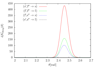
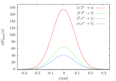
Figure 4: Emission characteristics of the attainable number of merged photons for our set-up driven by two 1PW-class lasers. The parameters of the incoming beams are chosen as $\theta^{\prime}=\pi$, $\phi^{\prime}=0$, $\theta^{\prime\prime}=1.23{\rm rad}$ and $\phi^{\prime\prime}=0$; the polarization of the pump beam is $\varphi=0$. The angle $\theta^{\prime\prime}$ maximizing the merged photon yield is visible in Fig. 3. Left panel: differential photon number ${\rm d}\mathcal{N}_{\rm Merg}(\theta)$ as a function of the polar angle $\theta$, with the corresponding energy and $\phi$ integrations performed over the full parameter regime. Right panel: ${\rm d}\mathcal{N}_{\rm Merg}(\phi)$ as a function of the polar angle $\phi$, with the corresponding energy and polar angle integrals performed over their full parameter regimes. From these plots we infer that the merged signal photons are predominantly emitted in the $\rm x$-$\rm z$ plane, at an outgoing polar angle of $\theta\approx 2.46{\rm rad}$. For two 10PW driver lasers, the number of merged photons increases by a factor of 1000.

Figure 4 displays the emission characteristics for the optimum geometry with $\theta^{\prime\prime}=1.23{\rm rad}$ as inferred from Fig. 3. The left panel shows the distribution of merged photons as a function of the polar angle $\theta$, while the right panel depicts the distribution as a function of $\phi$. In both cases Eq. (IV) has been integrated over the entire parameter range of the correspondingly remaining angle as well as the signal photon energy. These plots imply that the merged photons are emitted into a rather small solid angle element: they predominantly propagate in the $\rm x$-$\rm z$ plane at an outgoing polar angle of $\theta\approx 2.46{\rm rad}$ (this result is illustrated in the right panel of Fig. 3, where the dashed vector $\mathbf{k}$ has been chosen correspondingly). Most notably, for our specific set-up the requirements of momentum and energy conservation yield a maximum emission of signal photons into regions where the fields of both the pump and the probe beams essentially vanish. Such a constellation is most favorable for optimizing the signal to noise ratio. Note that a Gaussian beam focussed down to the diffraction limit, as exemplarily depicted in Fig. 3 (right panel), has an opening angle of $1/\pi\approx 0.31{\rm rad}$. The resulting emission of the signal into the “free field” area together with the comparatively large number of signal photons makes this scenario an ideal candidate to experimentally verify the nonlinear nature of the quantum vacuum. Note that the laser parameters employed here resemble the parameters of typical petawatt class optical laser facilities which are currently in operation. Facilities with even more intense laser beams are being projected and developed (see, e.g., Vulcan10PW ; OmegaEP ; ELI ; XCELS ).

For completeness let us note that it might prove experimentally challenging to realize a set-up with two exactly counter-propagating lasers as considered here, cf. Fig. 3 (right panel). Even though this set-up provides for a larger number of merged photons, it might be desirable to avoid counter-propagating beams for experimental purposes. Keeping the remaining experimental parameters fixed but taking, e.g., $\theta^{\prime}=\frac{3\pi}{4}$ and $\theta^{\prime\prime}=0.77{\rm rad}$ still yields a total number of $\mathcal{N}_{\rm Merg}\approx 11.7$ signal photons per laser shot (for s^′,f${}^{\prime\prime}\rightarrow$ s), emitted predominantly at $\theta=1.92{\rm rad}$. In summary, our merging proposal facilitates rather flexible experimental realizations without fine-tuning requirements for the geometry of the incoming pump and probe beams.

Let us finally compare the all-optical configuration considered here with the four-wave mixing scenario suggested in Lundstrom:2005za ; Lundin:2006wu . The latter scenario focuses on the mixing of three incident photon waves from the outset to address elastic photon-photon scattering with high power lasers. Both scenarios have the use of high-intensity lasers in common as well as the same underlying set of Feynman diagrams. A main difference is that we consider the merging of two photon waves in a pump field inhomogeneity which is not restricted to the electromagnetic field of a propagating laser beam. Our formalism generalizes straightforwardly to any inhomogeneous pump field. Moreover, in our approach we can naturally make contact with the constant crossed-field limit for the pump field configuration as well as read off the various selection rules which govern the photon merging process.

V Conclusions

We have investigated photon merging and splitting processes in inhomogeneous, slowly varying electromagnetic fields, based on the three-photon polarization tensor following from the Heisenberg-Euler effective action. The influence of inhomogeneities appear particularly promising in the context of high-intensity laser facilities. For the parameter range of a typical petawatt class laser as pump and a terawatt class laser as probe, we provide estimates for the numbers of signal photons attainable in an actual experiment. The combination of frequency upshifting, polarization dependence and scattering off the inhomogeneities yields an inherent signal-to-background separation. This may give rise to successful implementations of single-photon detection schemes and renders photon merging an ideal signature for the experimental exploration of nonlinear quantum vacuum properties.

The central theoretical tool for these results is the explicit representation of the three-photon polarization tensor at one-loop order for slowly varying, but otherwise arbitrary electromagnetic field backgrounds. This expression allows to analyze in detail the selection rules for photon splitting and merging in crossed fields. We have also been able to demonstrate how the well-established restrictions arising from selection rules in constant background fields are lifted in inhomogeneous background fields.

The framework laid out in this work is ideally suited to obtain analytical insights into three-photon interaction processes induced by vacuum fluctuations in the strong electromagnetic fields generated by high-intensity lasers. The relevance of inhomogeneities becomes obvious from the fact that photon splitting and merging processes in constant background fields are suppressed as $({\cal E}/{\cal E}_{\rm cr})^{6}$ in the ratio of the background field strength $\cal E$ to the critical field strength ${\cal E}_{\rm cr}$. This consequence of the Adler theorem can be circumvented by inhomogeneous background fields which allow for momentum and energy transfers between the probe photons and the background field. As a result, the suppression is decreased to only $({\cal E}/{\cal E}_{\rm cr})^{2}$.

As the our quantitative estimates for the number of attainable signal photons already yields a decent amount of merged signal photons per laser shot – even for already existing state-of-the-art $1{\rm PW}$ class high-intensity laser systems – we believe that photon merging can be a good candidate to detect and investigate the optical nonlinearities of the quantum vacuum for the first time.

References

- (1) H. Euler and B. Kockel, Naturwiss. 23, 246 (1935).
- (2) W. Heisenberg and H. Euler, Z. Phys. 98, 714 (1936), an English translation is available at [physics/0605038].
- (3) V. Weisskopf, Kong. Dans. Vid. Selsk., Mat.-fys. Medd. XIV, 6 (1936).
- (4) W. Dittrich and M. Reuter, Lect. Notes Phys. 220, 1 (1985).
- (5) W. Dittrich and H. Gies, Springer Tracts Mod. Phys. 166, 1 (2000).
- (6) M. Marklund and J. Lundin, Eur. Phys. J. D 55, 319 (2009) [arXiv:0812.3087 [hep-th]].
- (7) G. V. Dunne, Eur. Phys. J. D 55, 327 (2009) [arXiv:0812.3163 [hep-th]].
- (8) T. Heinzl and A. Ilderton, Eur. Phys. J. D 55, 359 (2009) [arXiv:0811.1960 [hep-ph]].
- (9) A. Di Piazza, C. Muller, K. Z. Hatsagortsyan and C. H. Keitel, Rev. Mod. Phys. 84, 1177 (2012) [arXiv:1111.3886 [hep-ph]].
- (10) G. V. Dunne, Int. J. Mod. Phys. A 27, 1260004 (2012) [Int. J. Mod. Phys. Conf. Ser. 14, 42 (2012)] [arXiv:1202.1557 [hep-th]].
- (11) R. Battesti and C. Rizzo, Rept. Prog. Phys. 76, 016401 (2013) [arXiv:1211.1933 [physics.optics]].
- (12) B. King and T. Heinzl, arXiv:1510.08456 [hep-ph].
- (13) J. S. Toll, Ph.D. thesis, Princeton Univ., 1952 (unpublished).
- (14) R. Baier and P. Breitenlohner, Act. Phys. Austriaca 25, 212 (1967); Nuov. Cim. B 47 117 (1967).
- (15) Z. Bialynicka-Birula and I. Bialynicki-Birula, Phys. Rev. D 2, 2341 (1970).
- (16) R. Karplus and M. Neuman, Phys. Rev. 83, 776 (1951).
- (17) S. Z. Akhmadaliev, et al., Phys. Rev. C 58, 2844 (1998).
- (18) S. Z. Akhmadaliev, et al., Phys. Rev. Lett. 89, 061802 (2002) [hep-ex/0111084].
- (19) L. Meitner and H. Koesters, Z. f. Physik 84, 137 (1933).
- (20) H. Bethe and F. Rohrlich, Phys. Rev. 86, 10 (1952).
- (21) S. L. Adler, Annals Phys. 67, 599 (1971).
- (22) R. N. Lee, A. I. Milstein and V. M. Strakhovenko, Phys. Rev. A 57, 2325 (1998) [hep-ph/9804386].
- (23) G. Cantatore [PVLAS Collaboration], Lect. Notes Phys. 741, 157 (2008); E. Zavattini et al. [PVLAS Collaboration], Phys. Rev. D 77, 032006 (2008) [arXiv:0706.3419 [hep-ex]]; F. Della Valle, U. Gastaldi, G. Messineo, E. Milotti, R. Pengo, L. Piemontese, G. Ruoso and G. Zavattini, arXiv:1301.4918 [quant-ph]; F. Della Valle, A. Ejlli, U. Gastaldi, G. Messineo, E. Milotti, R. Pengo, G. Ruoso and G. Zavattini, Eur. Phys. J. C 76, 24 (2016) [arXiv:1510.08052 [physics.optics]].
- (24) P. Berceau, R. Battesti, M. Fouche and C. Rizzo, Can. J. Phys. 89, 153 (2011); P. Berceau, M. Fouche, R. Battesti and C. Rizzo, Phys. Rev. A, 85, 013837 (2012) [arXiv:1109.4792 [physics.optics]]; A. Cadène, P. Berceau, M. Fouché, R. Battesti and C. Rizzo, Eur. Phys. J. D 68, 16 (2014) [arXiv:1302.5389 [physics.optics]].
- (25) G. Zavattini, F. Della Valle, A. Ejlli and G. Ruoso, arXiv:1601.03986 [physics.optics].
- (26) see HIBEF website: http://www.hzdr.de/db/Cms?pOid=35325&pNid=3214
- (27) T. Heinzl, B. Liesfeld, K. -U. Amthor, H. Schwoerer, R. Sauerbrey and A. Wipf, Opt. Commun. 267, 318 (2006) [hep-ph/0601076].
- (28) F. Karbstein, H. Gies, M. Reuter and M. Zepf, Phys. Rev. D 92, 071301 (2015) [arXiv:1507.01084 [hep-ph]].
- (29) H. -P. Schlenvoigt, T. Heinzl, U. Schramm, T. Cowan and R. Sauerbrey, Physica Scripta 91, 023010 (2016).
- (30) A. Di Piazza, K. Z. Hatsagortsyan and C. H. Keitel, Phys. Rev. Lett. 97, 083603 (2006) [hep-ph/0602039].
- (31) V. Dinu, T. Heinzl, A. Ilderton, M. Marklund and G. Torgrimsson, Phys. Rev. D 89, 125003 (2014) [arXiv:1312.6419 [hep-ph]]; Phys. Rev. D 90, 045025 (2014) [arXiv:1405.7291 [hep-ph]].
- (32) B. Marx, et al., Opt. Comm. 284, 915 (2011); Phys. Rev. Lett. 110, 254801 (2013).
- (33) B. King, A. Di Piazza and C. H. Keitel, Nature Photon. 4, 92 (2010) [arXiv:1301.7038 [physics.optics]]; Phys. Rev. A 82, 032114 (2010) [arXiv:1301.7008 [physics.optics]].
- (34) D. Tommasini and H. Michinel, Phys. Rev. A 82, 011803 (2010) [arXiv:1003.5932 [hep-ph]].
- (35) K. Z. Hatsagortsyan and G. Y. Kryuchkyan, Phys. Rev. Lett. 107, 053604 (2011).
- (36) E. Lundstrom, G. Brodin, J. Lundin, M. Marklund, R. Bingham, J. Collier, J. T. Mendonca and P. Norreys, Phys. Rev. Lett. 96, 083602 (2006) [hep-ph/0510076].
- (37) J. Lundin, M. Marklund, E. Lundstrom, G. Brodin, J. Collier, R. Bingham, J. T. Mendonca and P. Norreys, Phys. Rev. A 74, 043821 (2006) [hep-ph/0606136].
- (38) B. King and C. H. Keitel, New J. Phys. 14, 103002 (2012) [arXiv:1202.3339 [hep-ph]].
- (39) H. Gies, F. Karbstein and N. Seegert, New J. Phys. 15, 083002 (2013) [arXiv:1305.2320 [hep-ph]]; New J. Phys. 17, 043060 (2015) [arXiv:1412.0951 [hep-ph]].
- (40) F. Karbstein and R. Shaisultanov, Phys. Rev. D 91, 085027 (2015) [arXiv:1503.00532 [hep-ph]].
- (41) S. L. Adler, J. N. Bahcall, C. G. Callan and M. N. Rosenbluth, Phys. Rev. Lett. 25, 1061 (1970).
- (42) V. O. Papanyan and V. I. Ritus, Zh. Eksp. Teor. Fiz. 61, 2231 (1971) [Sov. Phys. JETP 34, 1195 (1972)].
- (43) V. O. Papanyan and V. I. Ritus, Zh. Eksp. Teor. Fiz. 65, 1756 (1973) [Sov. Phys. JETP 38, 879 (1974)].
- (44) R. J. Stoneham, J. Phys. A, 12, 2187 (1979).
- (45) V. N. Baier, A. I. Milshtein and R. Z. Shaisultanov, Sov. Phys. JETP 63, 665 (1986) [Zh. Eksp. Teor. Fiz. 90, 1141 (1986)].
- (46) V. N. Baier, A. I. Milshtein and R. Z. Shaisultanov, Phys. Rev. Lett. 77, 1691 (1996) [hep-th/9604028].
- (47) S. L. Adler and C. Schubert, Phys. Rev. Lett. 77, 1695 (1996) [hep-th/9605035].
- (48) A. Di Piazza, A. I. Milstein and C. H. Keitel, Phys. Rev. A 76, 032103 (2007) [arXiv:0704.0695 [hep-ph]].
- (49) V.P. Yakovlev, Zh. Eksp. Teor. Fiz. 51, 619 (1966) [Sov. Phys. JETP 24, 411 (1967)].
- (50) A. Di Piazza, K. Z. Hatsagortsyan and C. H. Keitel, Phys. Rev. Lett. 100, 010403 (2008) [arXiv:0708.0475 [hep-ph]]; Phys. Rev. A 78, 062109 (2008) [arXiv:0906.5576 [hep-ph]].
- (51) H. Gies, F. Karbstein and R. Shaisultanov, Phys. Rev. D 90, 033007 (2014) [arXiv:1406.2972 [hep-ph]].
- (52) F. Karbstein and R. Shaisultanov, Phys. Rev. D 91, 113002 (2015).
- (53) H. Gies and K. Langfeld, Nucl. Phys. B 613, 353 (2001) [arXiv:hep-ph/0102185]; H. Gies and K. Langfeld, Int. J. Mod. Phys. A 17, 966 (2002) [arXiv:hep-ph/0112198]; K. Langfeld, L. Moyaerts and H. Gies, Nucl. Phys. B 646, 158 (2002) [arXiv:hep-th/0205304]; H. Gies and L. Roessler, Phys. Rev. D 84, 065035 (2011) [arXiv:1107.0286 [hep-ph]]; D. Mazur and J. S. Heyl, Phys. Rev. D 91, 065019 (2015) [arXiv:1407.7490 [hep-th]].
- (54) J. S. Schwinger, Phys. Rev. 82, 664 (1951).
- (55) W. y. Tsai and T. Erber, Phys. Rev. D 12, 1132 (1975).
- (56) B. King, P. Böhl and H. Ruhl, Phys. Rev. D 90, 065018 (2014) [arXiv:1406.4139 [hep-ph]].
- (57) P. Böhl, B. King and H. Ruhl, Phys. Rev. A 92, 032115 (2015) [arXiv:1503.05192 [physics.plasm-ph]].
- (58) https://eli-laser.eu/
- (59) http://www.stfc.ac.uk/CLF/Facilities/Vulcan/The+Vulcan+10+Petawatt+Project/14684.aspx
- (60) http://www.lle.rochester.edu/omega_facility/omega_ep/
- (61) http://www.xcels.iapras.ru/