Spectral duality in elliptic systems, six-dimensional gauge theories and topological strings

Abstract

We consider Dotsenko-Fateev matrix models associated with compactified Calabi-Yau threefolds. They can be constructed with the help of explicit expressions for refined topological vertex, i.e. are directly related to the corresponding topological string amplitudes. We describe a correspondence between these amplitudes, elliptic and affine type Selberg integrals and gauge theories in five and six dimensions with various matter content. We show that the theories of this type are connected by spectral dualities, which can be also seen at the level of elliptic Seiberg-Witten integrable systems. The most interesting are the spectral duality between the XYZ spin chain and the Ruijsenaars system, which is further lifted to self-duality of the double elliptic system.

^a Lebedev Physics Institute, Moscow 119991, Russia
^b ITEP, Moscow 117218, Russia
^c Institute for Information Transmission Problems, Moscow 127994, Russia
^d National Research Nuclear University MEPhI, Moscow 115409, Russia
^e Institute of Nuclear Research, Moscow 117312, Russia

1 Introduction

Gauge theories with eight supercharges in 4d, 5d and 6d can be effectively analyzed from the string theory perspective. This view is natural if one wants to study deformations of these theories and understand their structure in geometric terms. Also this family of gauge theories turns out to be a focus point of several dualities, some of which are still in need of a full explanation.

One of these dualities is the AGT correspondence, relating partition functions of gauge theories to 2d CFT conformal blocks. It was first observed for 4d theories [1], then generalized to 5d [2] and very recently to 6d [3]. The AGT relation was motivated by the study of the worldvolume theory on the stack of M5 branes wrapping a Riemann surface, the bare spectral curve [4]. This geometric point of view naturally incorporated various properties of 4d $\mathcal{N}=2$ gauge theories: $S$-duality, Seiberg-Witten curve, BPS states counting and relation with integrable systems. Any geometric meaning of the AGT duality for 5d gauge theories, which features $q$-deformed 2d CFT, is not so manifest.

Gauge theories in five dimensions can be obtained using a different approach, the geometric engineering technique, which relates them to type IIB strings on the $(p,q)$-brane web [5, 6] or topological strings on toric Calabi-Yau three-folds. This approach allows for direct computation using the refined topological vertex technique [7, 8], and explicitly reproduces the Nekrasov partition function of gauge theories.

$(p,q)$-webs and toric CY backgrounds have a natural symmetry, the spectral [9, 10], or fiber-base, duality, which is also the $S$-duality of IIB strings. This duality connects gauge theories with different gauge groups and matter content, which, however, have the same partition functions and the same set of BPS particles: the instantons and $W$-bosons get exchanged. The spectral duality has been studied for linear quiver gauge theories [11] and for $SU(2)$ gauge theories with $N_{f}\leq 8$ fundamental matter multiplets [12].

It has also been understood that the spectral duality is closely related to the AGT duality. In [13] (see also [14]) the Dotsenko-Fateev (DF) integrals for conformal blocks of the $q$-deformed CFT [15, 16, 17] have been rewritten as sums over residues, each corresponding to a fixed point in the instanton moduli space of a 5d gauge theory. However, this gauge theory turned out to be not the theory related to the conformal block by the AGT duality, but rather its spectral dual. Thus, the AGT relation is obtained as action of the spectral duality on the DF integrals of the $q$-deformed CFT.

In [18], [19], [20] we initiated a program to better understand the relationship between 5d gauge theories, $q$-deformed conformal blocks and structure of refined topological string amplitudes on toric CY. Here we would like to extend our analysis to the compactified toric CY, which correspond to 6d gauge theories and to the elliptic deformation of the conformal algebra.

In the spirit of [19], we show how to combine the elementary building blocks, amplitudes of the refined topological string in order to obtain the measures of the DF-type integral representations of conformal blocks in various theories. In this way, we obtain the integrals for $W_{N}$ algebras (also known as $A_{N}$ $q$-Selberg integrals), toric $q$-deformed conformal blocks (featuring in the “elliptic AGT relations” [3]), conformal blocks corresponding to affine root systems (related to the 6d gauge theories), and the setup corresponding to the 6d theory with adjoint matter.

It is well-known that gauge theories we are considering correspond to the Seiberg-Witten integrable systems [21]-[33],[6]. In the case of compactified brane diagram, these integrable systems are of elliptic type. They include the elliptic Ruijsenaars, the XYZ spin chain and the still mysterious double elliptic integrable system [31]. We propose the spectral duality for these systems and make a few qualitative tests of it.

One motivation for going to 6d is to probe the $(2,0)$ 6d superconformal theory, which is thought to originate from coincident M5 branes. However, what we actually obtain is the $T$-dual theory, the $(1,1)$ 6d gauge theory. This is the dimensional reduction of the 10d minimal supersymmetric gauge theory, which upon further reduction gives the $\mathcal{N}=2$ theory in 5d and $\mathcal{N}=4$ theory in 4d. The $(1,1)$ gauge theory can also be thought of as a Kähler gravity theory, which is the target space description of the microscopic “quantum foam” geometry of topological strings [34]. The theory can be put in the 6d $\Omega$-background with three equivariant parameters $q_{1,2,3}$ corresponding to three elements of the Cartan subalgebra of $SO(6)$. The “instantons” of the 6d theory, fixed under these isometries are identified with the atoms of the melting crystal model, and the partition function of the gauge theory is identified with the index version of the topological vertex.

We start our discussion by reminding the brane descriptions of gauge theories in 4d, 5d, 6d and their relation to (refined) topological strings. We then provide an exhaustive list of possible topological string amplitudes (including compactified toric diagrams), which are suitable as building blocks for quiver gauge theories in 5d and 6d. We also generalize the dictionary obtained in [19] to these amplitudes and describe the corresponding Dotsenko-Fateev type integrals. Our approach to the DF integrals exploits also the “triality” between 5d gauge theories, 3d theories and $q$-deformed conformal blocks proposed in [13]. We interpret the sums over Young diagrams as the sums over residues and then investigate structure of the corresponding integral.

In the second part, we focus on one particular amplitude for the compactified CY, which corresponds to the 5d gauge theory with adjoint matter, or, employing the spectral duality, to the 6d linear quiver of $U(1)$ groups. We find here a close counterpart of the triality, which gives the affine version of the $q$-Selberg integrals. Investigating the pole structure of these integrals we encounter a new interesting phenomenon: the contour of integration does not encircle all the poles of the integrand. The meaning of the missing poles turns out to be quite remarkable: they correspond to instantons of the six-dimensional gauge theory enumerated by the plane partitions (3d Young diagrams). Even more remarkable is the fact that each residue exactly reproduces the equivariant $K$-theory index of the corresponding fixed point in the instanton moduli space of the $\mathcal{N}=(1,1)$ 6d theory [35, 36]. We also point out that the affine Selberg integrals and their generalizations, which we introduce, have a very nice cohomology limit, in which they turn into the 6d counterparts of the LMNS integrals [37]. Taking a further limit reduces the integrals to the standard 4d LMNS ones. Thus, our extended integral provides a simple explanation for the AGT relation between the two very different integral representations of the same quantity: the DF integrals (representing the conformal blocks) and the LMNS integrals (computing the Nekrasov partition function).

In the last part of the paper, we discuss the Seiberg-Witten integrable systems, corresponding to the gauge theories we have considered. We first recall the general idea of the integrable system construction, and then proceed to study action of the spectral duality on integrable systems a la [9]. We generalize the results known for the rational and trigonometric systems to the elliptic ones: the elliptic Ruijsenaars model, the XYZ spin chain, the double elliptic systems and their generalizations. We show that the spectral duality originating from the $(p,q)$-brane rotation indeed gives a nontrivial identification between different elliptic systems.

1.1 Brane pictures

For 4d theories the relevant brane construction is provided by Type IIA theory [38] (see also related subjects in [39]). To obtain a linear $U(N)^{M-1}$ gauge theory one considers a set of $M$ “vertical” NS5 branes extending in the $(x^{0},x^{1},x^{2},x^{3},x^{4},x^{5})$ directions and $N$ “horizontal” D4 branes suspended between them in the directions $(x^{0},x^{1},x^{2},x^{3},x^{6})$. The $(x^{5},x^{6})$ projection of this setting is shown in Fig. 1. On the segments of D4 branes suspended between each pair of adjacent NS5 branes lives a gauge theory with $U(N)$ gauge group, which is spontaneously broken down to $U(1)^{N}$ by the adjoint scalar vacuum averages $a^{(\alpha)}_{i}$. These averages are represented by the vertical distances between the D4 branes. The (asymptotic) distance between the two NS5 branes represent the complexified coupling constant $\Lambda_{\alpha}=-i\tau_{\alpha}=\frac{4\pi}{g^{2}_{\alpha}}-\frac{i\theta_{\alpha}}{2\pi}$ of the gauge group. The neighbouring gauge groups in the linear quiver are coupled through a bifundamental hypermultiplet. Its mass $m_{\mathrm{bif}}$ is given by the relative positions of the centers of masses of D4 branes to the left and to the right of the corresponding NS5 brane. There are $N$ semi-infinite D4 branes coming from the left — they correspond to $N$ fundamental matter fields with masses $m_{\mathrm{f},i}$ coupled to the first $U(N)$ gauge factor of the quiver. These branes can also be understood as arising from an additional gauge theory with vanishing coupling constant. Similarly $N$ branes extending to the right of the diagram correspond to $N$ antifundamental hypermultiplets with masses $\overline{m}_{\mathrm{f},i}$ coupled to the last gauge factor. One can make the hypermultiplets infinitely massive while simultaneously sending the gauge coupling to zero. This corresponds to the picture, where all the semi-infinite D4 branes are moved infinitely high or low. The D4 branes have tension, which bends the NS5 branes, so they are no longer asymptotically parallel to each other. This simply means that there is no well-defined coupling at high energies, and the theory is asymptotically free. Indeed, bending of NS5 branes can be found by solving for a minimal surface in 3d space spanned by $(x^{4},x^{5},x^{6})$. Thus, the brane diagram in Fig. 1 is only schematic — NS5 branes should be viewed as curved surfaces pulled by D4 branes. Away from D4 branes one gets $x^{6}(x^{4},x^{5})\sim\ln|x^{4}+ix^{5}|$ — characteristic behavior of an asymptotically free theory. If there are the same numbers of D4 branes pulling an NS5 brane to the left and to the right, then the tension is balanced and asymptotically one has $x^{6}(x^{4},x^{5})\sim\mathrm{const}$, so that the resulting gauge theory is conformal in the UV.

Figure 1: Type IIA brane diagram corresponding to $U(2)^{2}$ linear quiver.

To analyze the non-perturbative effects, such as instantons, in the gauge theory the picture has to be lifted to M-theory. The extra coordinate forms a circle $S^{1}_{R_{11}}$, which radius is proportional to Type IIA string coupling constant. Then, the NS5 and D4 branes are described by a single M5-brane, wrapping the complex Seiberg-Witten curve $\Sigma$, which should be holomorphic due to supersymmetry. The matter content, prepotential, BPS spectrum and global symmetries can be read off from the curve and the corresponding brane diagram. In particular, M2 branes suspended between the sheets of $\Sigma$ and wrapping special contours on it correspond to BPS particles in the gauge theory. Partition function of the gauge theory can be found by evaluating the periods of the Seiberg-Witten differential $\lambda$ over the Seiberg-Witten curve $\Sigma$.

Let us describe one more system associated with the brane picture: the Seiberg-Witten integrable system. The phase space of this system can be understood as follows. The family of Seiberg-Witten curves is parameterized by the Coulomb moduli of the gauge theory, which correspond to positions of the D4 branes in the Type IIA picture. These are the integrals of motion, or Hamiltonians of the integrable system. Thus, the Seiberg-Witten curve is identified with the spectral curve of the integrable system, which is the generating function of the Hamiltonians. For fixed values of the Hamiltonians, the system moves on a torus. This torus is given by the Jacobian of the Seiberg-Witten curve, so that the whole phase space is a torus fibration over the Coulomb branch of the gauge theory moduli space. The surprising fact is that Seiberg-Witten integrable systems can in fact be described very concretely and coincide with some classic integrable systems: e.g. for 4d $U(N)^{M-1}$ linear quiver it is given by the periodic $\mathfrak{gl}_{M}$ XXX spin chain with $N$ spins [26]. The masses of the hypermultiplets correspond to Casimir operators of the spins and the couplings enter the twist matrix of the chain.

Figure 2: Type IIA brane diagram corresponding to $U(3)$ theory with adjoint multiplet. Notice the cyclic identification of the lines on the left and right.

In a similar way one can consider gauge theories with adjoint matter. In this case the $x^{6}$ direction (horizontal in Fig. 1) should be compactified on a circle $S^{1}_{R_{6}}$, so that the D4 branes no longer extend to infinity on the left and right margins of the page, but wrap the $S^{1}_{R_{6}}$ circle with both ends attached to a single NS5 brane. The resulting arrangement is shown in Fig. 2. By compactifying diagrams with more NS5 branes, one gets a “necklace” quiver of gauge groups coupled by bifundamentals. For the resulting gauge theory to be well defined in the UV one has to make all the gaps between NS5 branes expanding asymptotically, or staying constant. The only way to actually obey this constraint is to make the number of D4 branes suspended between each two NS5 branes the same, which gives the $U(N)^{M}$ quiver. The integrable system corresponding to the 4d $U(N)$ theory with adjoint matter is $N$-particle elliptic Calogero model [23], and for necklace quivers it is a certain multipoint generalization of Calogero system [10]. The mass of the adjoint multiplet corresponds to the Calogero coupling constant and the gauge theory coupling constant is encoded in the elliptic parameter of the system.

One can also compactify the $x^{4}$ direction (which is perpendicular to the plane of Figs. 1, 2). To get the gauge theory interpretation of this setup we perform $T$-duality along the resulting circle $S^{1}_{1/R_{4}}$. Under $T$-duality Type IIA theory turns into Type IIB, which has odd instead of even D-branes. Thus, after $T$-duality, D4 branes, which were suspended between the NS5 branes and spanned $(x^{0},x^{1},x^{2},x^{3},x^{6})$, being transverse to $S^{1}_{1/R_{4}}$, become D5-branes, wrapped over $S^{1}_{R_{4}}$ and spanning $(x^{0},x^{1},x^{2},x^{3},x^{4},x^{6})$. The worldvolume theory on D5 branes is generally a six-dimensional gauge theory. However, in the $x^{6}$ direction the brane has a finite span $\Lambda$, so the resulting low energy theory is five-dimensional gauge theory on $(x^{0},x^{1},x^{2},x^{3},x^{4})\in\mathbb{R}^{4}\times S^{1}_{R_{4}}$. However, as in the NS5-D4 system discussed above, we have to include brane tension in our picture. The difference with the D4 case is that now we have to solve the minimal surface condition in two-dimensional space $(x^{5},x^{6})$, so the resulting surface is always a straight line (this answer also follows from supersymmetry constraints). D5 branes are represented by horizontal lines and called $(0,1)$ branes, and NS5 branes are vertical lines, or $(1,0)$ in this setting. When $(0,1)$ and $(1,0)$ branes merge one has to balance the tension, so the resulting brane is can be neither vertical, nor horizontal. In fact the tensions of $(0,1)$ and $(1,0)$ branes can be made the same by a suitable choice of $x^{5}$ and $x^{6}$ scales, and we will assume this choice throughout our discussion. The bound state of $(0,1)$ and $(1,0)$ branes has unit slope, and is called the $(1,1)$ brane. All other bound states can be obtained in a similar fashion and the whole web of branes in the $(x^{5},x^{6})$ plane is called the Type IIB $(p,q)$-brane web [5]. The example of a brane web is depicted in Fig. 3. Notice that the angles of the branes are related to their charges — which are conserved in any brane merger. The moduli of the gauge theory correspond to the lengths of the edges, which we denote by $Q_{i}$. More concretely, in the example shown in Fig. 3 $Q_{m,i}$ correspond to the gauge theory masses, $Q_{F,i}$ encode the vacuum moduli and $Q_{B,i}$ are related to the couplings $\Lambda_{i}$. Notice that in this picture the vacuum averages, masses and coupling constants all appear on the same footing. Moreover the $S$-duality of the type IIB theory turns $(1,0)$ brane into a $(0,1)$ brane, thus eliminating the asymmetry between the vertical and horizontal directions.

Rotation of the brane web, or $S$-duality in Type IIB language, which is obviously a symmetry of the theory, corresponds to a nontrivial duality between 5d gauge theories, corresponding to the web. Indeed, for $M$ vertical branes intersecting with $N$ horizontal branes one has the $U(N)^{M-1}$ linear quiver, while for a rotated web it should be $U(M)^{N-1}$. The relation between two gauge theories is given by the spectral duality. One can understand this duality as the map on the space of BPS states of the theories, taking the $W$-bosons of one theory into the instantons of the other and vice versa. The masses of the BPS states are given by $M_{BPS}=|Z|\sim a_{i}n_{i}+\Lambda_{i}k_{i}+\ldots$, where $n_{i}$ are $U(1)^{N}$ charges and $k_{i}$ are instanton numbers with respect to $U(N)^{M}$. From this expression we see that the spectral duality maps Coulomb moduli of one theory to couplings of the dual theory. This is also evident from the brane web, since vertical and horizontal distances correspond to Coulomb moduli and couplings respectively.

The integrable system corresponding to the 5d $U(N)^{M-1}$ linear quiver gauge theory is the periodic $U_{q}(\mathfrak{gl}_{M})$ XXZ spin chain with $N$ spins [26]. As in the XXX case, masses and couplings of the gauge theory are written in terms of Casimir operators and twist matrix of the spin chain. Notice that spectral duality is also a nontrivial duality of the two spin chains: the $U_{q}(\mathfrak{gl}_{M})$ chain with $N$ spins is mapped onto the $U_{q}(\mathfrak{gl}_{N})$ chain with $M$ spins [9]. The spectral curves of the two systems coincide, while the Hamiltonians are expressed through each other and the parameters of the systems.

Again, as in the Type IIA case, considered above, to obtain the non-perturbative description of the $5d$ gauge theory, one has to lift the $(p,q)$-web to M-theory. We start from Type IIB theory on $\mathbb{R}^{9}\times S^{1}_{R_{4}}$, which is equivalent to M-theory on $\mathbb{R}^{9}\times\mathbb{T}^{2}$ with $\mathrm{Vol}(\mathbb{T}^{2})=R_{4}$. A $(p,q)$-brane of Type IIB is M5 brane wrapping the $(p,q)$-cycle on $\mathbb{T}^{2}$. By a chain of dualities one can transform this brane picture into a purely geometric background without any branes, namely the toric Calabi-Yau threefold [40], so that the whole setup looks like $\mathbb{R}^{4}\times\mathrm{CY}_{3}\times S^{1}$. $\mathrm{CY}_{3}$ is a $\mathbb{T}^{3}$-fibration degenerating over the edges and vertices of the toric diagram $\mathcal{T}\in\mathbb{R}^{3}$, which completely determines the geometry and is identified with the brane web from Type IIB. Finite edges of the diagram represent the two-spheres inside the CY, and, instead of the lengths of brane segments, the relevant parameters are Kähler moduli of these spheres, which we also denote by $Q_{i}$. Notice that not all the edge lengths are independent: one needs to impose constraints, so that all the cycles on the diagram are indeed closed. In particular, each cycle imposes two constraints, corresponding to horizontal and vertical projections. On Fig. 3 we label only the independent lengths.

Figure 3: Type IIB $(p,q)$-brane web, or CY toric diagram, corresponding to 5d $U(2)^{2}$ linear quiver.

Toric or web diagrams can be compactified in the same way as the type IIA brane diagram. Again, the edges of the picture become identified and some of the branes wrap the resulting cycle, as shown on Fig. 4, resulting in a $5d$ gauge theory with adjoint (or more generally necklace quiver of bifundamental) matter. Moreover, since there is no difference between the horizontal and vertical directions in this picture, one can consider the vertical compactification as well (see Fig. 4). The vertical compactification corresponds to the 6d gauge theory with fundamental matter. The important point here is that since the vertical direction is compact, one cannot send the semi-infinite D5 branes up or down indefinitely, and only $U(N)$ gauge theories with exactly $2N$ fundamental multiplets are allowed. Also, there is a constraint that the sum of all the masses is equal to the sum of all the vacuum moduli. In the language of the gauge theory this constraint can be understood as the anomaly cancellation condition for large gauge transformations.

Figure 4: Type IIB $(p,q)$-brane web, or CY toric diagram, corresponding to 5d $U(3)$ gauge theory with adjoint multiplet. Notice the cyclic identification of the lines on the left and right.

Notice that spectral duality still acts on the compactified diagram. However, the dual gauge theories are now of different space-time dimension: one is the 5d $U(N)^{M}$ necklace quiver theory and the other is the 6d $U(M)^{N-1}$ linear quiver. The BPS states of the two theories are identified in the same way, as for the 5d linear quivers discussed above.

In the language of integrable systems spectral duality gives a new nontrivial identification between different elliptic systems. More concretely, 5d $U(N)^{M}$ necklace quiver theory corresponds to multipoint generalization of elliptic Ruijsenaars system, while 6d $U(M)^{N-1}$ linear quiver is described by the XYZ spin chain. The two gauge theories are dual, and thus the integrable systems are also dual, in the same way as the XXZ spin chains in the example discussed above. We conclude that the XYZ spin chain is spectral dual to the multipoint elliptic Ruijsenaars model.

Naturally one can also compactify both horizontal and vertical directions of the toric diagram, and obtain the 6d necklace quiver theory. This theory seems in many ways special. In particular, the corresponding Seiberg-Witten integrable system is of double elliptic type, i.e. the Hamiltonians depend elliptically both on the coordinates and momenta. This system is currently a subject of intense investigation [31]. We only mention here that, since the doubly compactified toric diagram can be rotated to get another doubly compactified diagram, different double elliptic systems should be connected by the spectral duality.

1.2 From pictures to formulas

For concrete computations, we use the relation between M-theory on $\mathrm{CY}_{3}\times\mathbb{R}^{4}\times S^{1}$ and (refined) topological strings on $\mathrm{CY}_{3}$, where the (refined) topological vertex technique can be used. Let us describe the recipe to obtain the partition function from the toric diagram.

To each 3-valent vertex of the toric diagram one assigns a 3-index object $C_{ABC}(q,t)$, where $A$, $B$ and $C$ are Young diagrams, residing on the three edges adjacent to the vertex, and the two parameters of the vertex, $q=e^{-\epsilon_{2}R_{5}}$, $t=q^{\beta}=e^{\epsilon_{1}R_{5}}$, are related to $\Omega$-deformation parameters $(\epsilon_{1},\epsilon_{2})$ of the corresponding 5d gauge theory on $\mathbb{R}^{4}\times S^{1}_{R_{5}}$. In topological strings $q$ is also the exponentiated string coupling $q=e^{-g_{s}}$, so that $R_{5}$ can also be understood as the radius of the M-theory circle. The ordering of indices in the refined topological vertex $C_{ABC}(q,t)$ depends on the extra labels of the adjacent edges. For toric manifolds, which we consider, each vertex has one edge with preferred direction (marked with double stroke) and two other labelled by $t$ and $q$, see [8]:

$$C_{ABC}(t,q)=\quad\parbox{56.9055pt}{ \includegraphics[width=56.9055pt]{figures/ref-vertex-crop}}\quad=q^{\frac{||B||^{2}+||C||^{2}}{2}}t^{-\frac{||B^{\mathrm{T}}||^{2}+||C^{\mathrm{T}}||^{2}}{2}}M^{(q,t)}_{C}\left(t^{-\rho}\right)\times\\ \times\sum_{D}\left(\frac{q}{t}\right)^{\frac{|D|+|A|-|B|}{2}}\chi_{A^{\mathrm{T}}/D}\left(q^{-C}t^{-\rho}\right)\chi_{B/D}\left(t^{-C^{\mathrm{T}}}q^{-\rho}\right),$$ (1)

To each internal edge of the toric diagram one assigns the (complexified) Kähler parameter $Q$ of the corresponding two-cycle in the CY. If the two vertices are joined by an edge, then the corresponding indices are contracted with the “propagator” $G^{AB}(Q,q,t)$:

$$G^{AB}(Q,t,q)=\quad\parbox{56.9055pt}{ \includegraphics[width=56.9055pt]{figures/prop-crop}}\quad=\delta_{AB}Q^{|A|}\left((-1)^{|A|}q^{\frac{||A^{\mathrm{T}}||^{2}+|A|}{2}}t^{-\frac{||A||^{2}+|A|}{2}}\right)^{n},$$ (2)

$$\widetilde{G}^{AB}(Q,t,q)=\quad\parbox{56.9055pt}{ \includegraphics[width=56.9055pt]{figures/prop2-crop}}\quad=\delta_{AB}Q^{|A|}\left((-1)^{|A|}t^{\frac{||A^{\mathrm{T}}||^{2}}{2}}q^{-\frac{||A||^{2}}{2}}\right)^{n},$$ (3)

where $n$ is the framing factor, depending on the relative orientation of the adjacent edges. Notice that the $t$ and $q$ marks should be different on the two sides of the propagator. The total closed string partition function corresponding to a diagram is given by the appropriate contraction of the propagators with the vertices. One can also leave some of the sums over the diagrams unevaluated, to obtain the open string amplitude. In this case, some of the external edges will contain the Young diagram labels, corresponding to the open string boundary conditions on the Lagrangian brane intersecting the corresponding leg of the diagram.

Compactification of the toric diagram introduces a new parameter — which can be though as either the coupling constant $\tau$ of the theory with adjoint hypermultiplet (similarly to Fig. 2, where it was given by $\Lambda$), or as the compactification radius $R_{6}$ of the 6d theory. This parameter is encoded in the Kähler parameter of the corresponding edge. For example, in Fig. 4 the (exponentiated) coupling constant is given by $Q_{\tau}=Q_{B}Q_{m}$. Notice that in the CY construction of gauge theories there is essentially no difference between the 5d theory with adjoint matter (e.g. in Fig. 4) or a 6d theory with fundamental matter (as e.g. in Fig. 5) — which is just another manifestation of the spectral duality.

Figure 5: Type IIB $(p,q)$-brane web corresponding to 6d $U(3)$ gauge theory with 6 fundamental multiplets. The compactification radius is given by $e^{-\epsilon_{2}R_{6}}=\prod_{a=1}^{3}Q_{m,a}Q_{F,a}$.

We also observe a new curios feature of the compactified diagrams [20]. If we consider the diagram corresponding to $U(1)$ gauge theory with adjoint matter, we get extra poles in the corresponding DF integral. Encircling these poles we arrive at the 6d $(1,1)$ gauge theory on $\mathbb{R}^{6}_{q_{1},q_{2},q_{3}}$ with three equivariant parameters. Two of these parameters are the equivariant parameters of the original gauge theory, while the third one is given by the mass of the adjoint multiplet. The partition function of this theory on $\mathbb{C}^{3}=\mathbb{R}^{6}$ computes the index topological vertex [36] with external diagrams all empty. One can hope that one more compactification of the brane diagram will give index vertex with nonzero external legs.

1.3 A primer: 5d $SU(2)$ theory and $q$-Virasoro 4-point conformal block

The 4-point conformal block [41] provided by the Dotsenko-Fateev (conformal) matrix model [15, 16, 17] and AGT related [1] to the $N_{f}=4$ $SU(2)$ SUSY gauge theories [42, 43], is associated with the square brane diagram [4].

The Kähler parameters of the diagram are related to gauge theory parameters as follows:

$$Q_{F}=q^{2a},\qquad Q^{\pm}_{1}=q^{-m_{1}^{\pm}-a},\qquad Q^{-}_{2}=q^{m_{2}^{\pm}-a},\qquad Q_{B}=\Lambda q^{2a}$$ (4)

Here $a$ is the Coulomb modulus of the gauge theory $m_{1,2}^{\pm}$ are the masses of the four fundamental hypermultiplets and $\Lambda$ is the exponentiated complexified coupling constant.

Figure 6: Toric diagram corresponding to the four-point $q$-deformed conformal block and $5d$ $U(2)$ gauge theory with four fundamentals.

The DF representation reads

$$\mathcal{B}_{4}^{\mathrm{sphere}}(\Delta_{\mathrm{int}}=a,\vec{\Delta}_{\mathrm{ext}},c=1-6(b^{2}-b^{-2}),z=\Lambda)=\int\prod_{i=1}^{N}dx_{i}\,\Delta^{2\beta}(x)V_{\alpha_{0}}(0,x)V_{\alpha_{\Lambda}}(\Lambda,x)V_{\alpha_{1}}(1,x)$$ (5)

where $\Delta(x)$ is the Vandermonde determinant and $V_{\alpha}(z,x)=\prod_{i=1}^{N}(z-x_{i})^{b\alpha}$. On the other hand the block should be given by a sum over a quadruple of partitions — each corresponding to internal edge of the diagram.

The hidden quadruple symmetry is revealed if Yang-Mills theory is lifted to 5 dimensions [28, 29] and ordinary Dotsenko-Fateev integrals are substituted [17] by Jackson sums

$$\int_{0}^{1}f(x)dx\longrightarrow(1-q)\sum_{n}q^{n}f(q^{n})$$ (6)

with discretization parameter $q=e^{-\epsilon_{2}R_{5}}$. The Vandermonde determinants in the measure are replaced by their $(q,t)$-deformation:

$$\Delta^{(2\beta)}(x)\longrightarrow\prod_{m=1}^{\beta}\prod_{i,j=1}^{N}(x_{i}-q^{m-1}x_{j})=\prod_{i,j=1}^{N}\prod_{m=0}^{\infty}\frac{x_{i}-q^{m}x_{j}}{x_{i}-q^{m}tx_{j}}$$ (7)

with $t=q^{\beta}$. All the quantities in matrix model are analytically continued from integer values of $N$ and $\beta$, what is made unambiguously due to Selberg nature of the integrals [44]. This quadruple decomposition is recently presented in some detail in [19] based on the number of previous developments [44, 45, 46, 16, 47, 17, 18], see sec. 2.1.1 below. The group theory symmetry behind the whole picture [21] is encoded in the 2-site $U_{q}(\mathfrak{gl}_{2})$ XXZ spin chain integrable system [6, 27] (reduced to XXX in $4d$, when $q=1$ [24]).

As evident from Fig. 6, the diagram is very symmetric. Some symmetry is simple consequence of the symmetries in the matter content of the corresponding gauge theory, e.g. reflections along the horizontal and vertical lines correspond to renaming of the fundamental hypermultiplets $m_{1}^{\pm}\leftrightarrow m_{2}^{\pm}$ and charge conjugation respectively. Also, in the CFT language these symmetries are related to the $z\to z^{-1}$ symmetry and renumbering of the primary fields in the conformal block.

However, reflection along the diagonal (or, equivalently rotation by $\frac{\pi}{2}$) is not evident neither in the gauge theory, nor in the CFT. In fact, it corresponds to the spectral duality between two $U(2)$ gauge theories, such that Coulomb modulus $q^{2a}$ is interchanged with the coupling constant $\Lambda$. For the conformal blocks it is the duality between two four-point conformal blocks of the $q$-Virasoro algebra, in which the cross-ratio of positions is interchanged with the momentum of the intermediate field.

Let us describe this peculiar duality in more detail. Conformal block can be decomposed into a sum over intermediate states, and for certain very specific choice of basis — the basis of generalized Macdonald polynomials — labelled by pairs of Young diagrams, the resulting decomposition reproduces the “vertical cut” sum over $A$ and $B$ diagrams in Fig. 6. Moreover, the decomposition is also equal to the Nekrasov partition function and thus we get the following equality between the topological string partition function, conformal block and Nekrasov partition function:

$$\underline{Z_{\text{top string}}}=\sum_{A,B}\Lambda^{|A|+|B|}\langle V_{\alpha_{0}}(0)V_{\alpha_{\Lambda}}(1)|A,B,\Delta_{\mathrm{int}}\rangle\langle A,B,\Delta_{\mathrm{int}}|V_{\alpha_{1}}(1)V_{\alpha_{\infty}}(\infty)\rangle=\underline{\mathcal{B}_{4}^{\mathrm{sphere}}(\Delta_{\mathrm{ext}},\Delta_{\mathrm{int}},\Lambda)}=\\ =\sum_{A,B}\frac{z_{\mathrm{fund}}(a,m_{i}^{+},A,B)z_{\mathrm{fund}}(a,m_{i}^{-},A,B)}{z_{\mathrm{vect}}(a,A,B)}=\underline{Z_{\mathrm{Nek}}(a,m_{i}^{\pm},\Lambda)}$$ (8)

Expressing the $q$-deformed conformal block $\mathcal{B}_{4}$ in the DF form we get a discrete sum, which also turns out to be just the “horizontal cut” sum over $R_{\pm}$ in Fig. 6. Naturally, since the diagram is symmetric, this sum is also a Nekrasov decomposition of a certain gauge theory, though it is different from the one featuring in Eq. (8) — it is its spectral dual. We have:

$$\underline{Z_{\text{top string}}}=\sum_{R_{+},R_{-}}\left.\left[\Delta^{2\beta}(x)V_{\alpha_{0}}(0,x)V_{\alpha_{\Lambda}}(\Lambda,x)V_{\alpha_{1}}(1,x)\right]\right|_{x_{\pm,i}=q^{R_{\pm,i}+1}t^{N_{\pm-i}}}=\underline{\mathcal{B}_{4}^{\mathrm{shpere}}(\Delta_{\mathrm{ext}},\Delta_{\mathrm{int}},\Lambda)}=\\ =\sum_{R_{+},R_{-}}\Lambda_{\mathrm{d}}^{|R_{+}|+|R_{-}|}\frac{z_{\mathrm{fund}}(a_{\mathrm{d}},m_{\mathrm{d},i}^{+},A,B)z_{\mathrm{fund}}(a_{\mathrm{d}},m_{\mathrm{d},i}^{-},A,B)}{z_{\mathrm{vect}}(a_{\mathrm{d}},A,B)}=\underline{Z_{\mathrm{Nek}}(a_{\mathrm{d}},m_{\mathrm{d},i}^{\pm},\Lambda_{\mathrm{d}})}$$ (9)

In the last line the parameters of the Nekrasov function are dual, in particular the Coulomb moduli and coupling constant are exchanged.

Spectral duality acts on the topological vertices trivially only for $t=q$. In the refined case, $t\neq q$, and the vertices transform nontrivially under the rotation of the diagram, since the preferred direction also changes (see (1)). However, in this case one can understand the algebraic meaning of the duality.

Instead of considering rotation of the brane diagram, one can consider the rotation of the preferred direction. Different choices of the preferred direction correspond to different choices of basis in the tensor product of Fock modules corresponding to the legs of the diagram. For preferred direction along the legs the basis $|A,B,\Delta\rangle$ is the one appearing in the decomposition (8). For an orthogonal choice of the preferred direction, the basis is factorized $|A\rangle\otimes|B\rangle$. The change of basis from $|A,B,\Delta\rangle$ to the factorized basis $|A\rangle\otimes|B\rangle$ is performed using the generalized Kostka functions, described in [19]. We will return to this point when we describe the action of spectral duality for the compactified diagram.

2 DF measures from toric diagram

How do the DF measures for different conformal blocks arise from the toric diagrams? We show how to glue them from the elementary building block

$$Z\left(\left.\begin{smallmatrix}&P&\\ A&&B\\ &R&\end{smallmatrix}\right|Q,q,t\right)\quad=\quad\parbox{79.6678pt}{\includegraphics[width=79.6678pt]{figures/conifold-crop}}=Z_{\varnothing}(Q)q^{\frac{||R||^{2}-||P||^{2}}{2}}t^{\frac{||P^{\mathrm{T}}||^{2}-||R^{\mathrm{T}}||^{2}}{2}}\left(\frac{q}{t}\right)^{\frac{|A|-|B|}{2}}\times\\ \times M_{R}^{(q,t)}(t^{-\rho})M_{P^{\mathrm{T}}}^{(t,q)}(q^{-\rho})\prod_{i,j\geq 1}\prod_{k\geq 0}\frac{\left(1-q^{k}\sqrt{\frac{q}{t}}Qq^{R_{i}-P_{j}}t^{j-i+1}\right)\left(1-q^{k}\sqrt{\frac{q}{t}}Qt^{j-i}\right)}{\left(1-q^{k}\sqrt{\frac{q}{t}}Qq^{R_{i}-P_{j}}t^{j-i}\right)\left(1-q^{k}\sqrt{\frac{q}{t}}Qt^{j-i+1}\right)}\times\\ \times(-Q)^{|A|}\sum_{C}\chi_{A/C}\left(p_{n}\left(\sqrt{\frac{q}{t}}q^{-P}t^{-\rho}\right)-p_{n}(Q^{-1}q^{-R}t^{-\rho})\right)\chi_{B/C}\left(\frac{1-t^{n}}{1-q^{n}}\left[p_{n}\left(Qq^{R}t^{\rho}\right)-p_{n}(\sqrt{\frac{q}{t}}q^{P}t^{\rho})\right]\right)=\\ =\mathcal{N}M_{R}^{(q,t)}(t^{-\rho})M_{P^{\mathrm{T}}}^{(t,q)}(q^{-\rho})G_{RP}^{(q,t)}\left(\sqrt{\frac{q}{t}}Q\right)\times\\ \times\sum_{C}(-Q)^{|C|}\chi_{A^{\mathrm{T}}/C^{\mathrm{T}}}\left(p_{n}(t^{-\rho}q^{-R})-p_{n}\left(\sqrt{\frac{q}{t}}Qt^{-\rho}q^{-P}\right)\right)\chi_{B/C}\left(p_{n}(q^{-\rho}t^{-P^{\mathrm{T}}})-p_{n}\left(\sqrt{\frac{t}{q}}Qq^{-\rho}t^{-R^{\mathrm{T}}}\right)\right)$$ (10)

where $Z_{\varnothing}(Q)=Z\left(\left.\begin{smallmatrix}&\varnothing&\\ \varnothing&&\varnothing\\ &\varnothing&\end{smallmatrix}\right|Q,q,t\right)$ and $\mathcal{N}$ collects both the factors independent of the external diagrams $A$, $B$, $R$ and $P$ and framing factors which cancel when several amplitudes are glued together. When gluing two four-point amplitudes we use the identity (77).

It is possible to contract the amplitudes (10) in many different ways, and in the next several sections we will investigate all these possibilities. First of all, there are planar rectangular webs. They correspond to 5d linear quiver gauge theories with gauge groups $U(N)^{M}$. One can compactify the rectangle by identifying the opposite edges. Then, one gets either 6d linear quiver gauge theory or 5d necklace quiver, depending on the orientation of the identified edges. The two descriptions are spectral dual to each other, since they turn into one another by $\frac{\pi}{2}$ rotation of the brane diagram. Identifying both vertical and horizontal edges of the rectangle give the 6d necklace quiver gauge theory. These theories are spectral self-dual in a sense that the 6d theory with gauge group $U(N)^{M}$ is dual to the theory with gauge group $U(M)^{N}$. This generalizes the familiar result for 5d theories [11].

The classification of different compactifications/deformations and the respective measures is summarized in the table:

	Sphere	Torus
algebra	Selberg	Elliptic Selberg
$q$-deformed algebra	$q$-Selberg	Elliptic $q$-Selberg
doubly-deformed algebra	Affine Selberg	Elliptic affine Selberg

In each case there can be either Virasoro or $W_{M}$-algebra conformal block, corresponding to $A_{1}$ or $A_{M-1}$ Selberg measure. There can also be multiple vertex operator insertions in the integral. The number of these insertions and the rank of the $W_{M}$ algebra are related by the spectral duality.

2.1 $q$-deformed spherical block

The block is given by multiple contour integrals, each corresponding to a primary field insertion. These integrals can be evaluated by residues [13] and the poles are enumerated by Young diagrams, so that the resulting expressions coincide with the combinations of four-point topological string amplitudes. The alternative approach is to write down the sum instead of an integral from the very beginning. This sum is then called the Jackson $q-$integral and is defined as

$$\int_{0}^{a}d_{q}xf(x)=(1-q)\sum_{n\geq 0}q^{n}af(q^{n}a)$$ (11)

2.1.1 Virasoro conformal block

In this case the elementary building block of the DF integral is the $q$-Selberg average:

$$\langle f(x)\rangle_{q,t}=\int_{0}^{1}d_{q}^{N}x\,\Delta^{(q,t)}(x)\prod_{i=1}^{N}x_{i}^{u}\prod_{k=0}^{v-1}(1-q^{k}x_{i})f(x_{i}),$$ (12)

where the essential part of the measure is the $(q,t)$-Vandermonde

$$\Delta^{(q,t)}(x)=\prod_{i\neq j}\prod_{k\geq 0}\frac{1-q^{k}\frac{x_{i}}{x_{j}}}{1-tq^{k}\frac{x_{i}}{x_{j}}}=\prod_{i\neq j}\prod_{k=0}^{\beta-1}\left(1-q^{k}\frac{x_{i}}{x_{j}}\right).$$ (13)

It corresponds to the following combination of four-point amplitudes:

$$\parbox{113.81102pt}{\includegraphics[width=113.81102pt]{figures/q-sphere-vir-crop}}\quad=\mathcal{N}(-Q_{m,1})^{|A|}(-Q_{m,2})^{|C|}\sum_{R}\left(\sqrt{\frac{t}{q}}Q_{F}\right)^{|R|}\times\\ \times\prod_{k=0}^{\beta-1}\prod_{i\neq j\geq 1}\frac{\left(1-q^{k}\frac{x_{R,i}}{x_{R,j}}\right)\left(1-q^{k}Q_{m,1}Q_{m,2}\frac{t^{N-i}}{t^{N-j}}\right)}{\left(1-q^{k}\sqrt{\frac{q}{t}}Q_{m,1}\frac{t^{N-i}}{x_{R,j}}\right)\left(1-q^{k}\sqrt{\frac{q}{t}}Q_{m,2}\frac{x_{R,i}}{t^{N-j}}\right)}\times\\ \times\sum_{E,F}\chi_{A/E}\left(p_{n}\left(\sqrt{\frac{q}{t}}t^{-\rho}\right)-p_{n}\left(Q_{m,2}^{-1}t^{N+\frac{1}{2}}x_{R}^{-1}\right)\right)\chi_{B/E}\left(\frac{1-t^{n}}{1-q^{n}}\left(p_{n}\left(Q_{m,2}t^{-\frac{1}{2}-N}x_{R}\right)-p_{n}\left(\sqrt{\frac{q}{t}}t^{\rho}\right)\right)\right)\times\\ \times\chi_{C/F}\left(p_{n}\left(\sqrt{\frac{q}{t}}t^{N+\frac{1}{2}}x_{R}^{-1}\right)-p_{n}\left(Q_{m,1}^{-1}t^{-\rho}\right)\right)\chi_{D/F}\left(\frac{1-t^{n}}{1-q^{n}}\left(p_{n}\left(Q_{m,1}t^{\rho}\right)-p_{n}\left(\sqrt{\frac{q}{t}}t^{-\frac{1}{2}-N}x_{R}\right)\right)\right)$$ (14)

where $x_{R,i}=q^{R_{i}+1}t^{N-i}$ and $\mathcal{N}$ is a normalization constant independent of the diagrams $A$, $B$, $C$, $D$. To get the correct $q$-Selberg measure we have to set $\sqrt{\frac{q}{t}}Q_{m,1}=q^{-v}t^{-N}$, $\sqrt{\frac{q}{t}}Q_{m,2}=t^{N}$, and $Q_{F}=q^{u+v+\frac{1}{2}}t^{-\frac{1}{2}}$. Let us understand the structure of the topological string amplitude. The $(q,t)$-Vandermonde appears in the second line. The product over $i$ and $j$ is in fact finite for the discrete choice of the Kähler parameters we have made, since most terms in the numerator and the denominator cancel with each other. After the dust settles we get the residues of the $q$-Selberg measure:

$$\left(\sqrt{\frac{t}{q}}Q_{F}\right)^{|R|}\prod_{k=0}^{\beta-1}\prod_{i\neq j\geq 1}\frac{\left(1-q^{k}\frac{x_{R,i}}{x_{R,j}}\right)\left(1-q^{k}Q_{m,1}Q_{m,2}\frac{t^{N-i}}{t^{N-j}}\right)}{\left(1-q^{k}\sqrt{\frac{q}{t}}Q_{m,1}\frac{t^{N-i}}{x_{R,j}}\right)\left(1-q^{k}\sqrt{\frac{q}{t}}Q_{m,2}\frac{x_{R,i}}{t^{N-j}}\right)}=\\ =\frac{\Delta^{(q,t)}(x_{R})\prod_{i=1}^{N}x_{R,i}^{u}\prod_{k=0}^{v-1}\left(1-q^{k}x_{R,i}\right)}{\Delta^{(q,t)}(x_{\varnothing})\prod_{i=1}^{N}x_{\varnothing,i}^{u}\prod_{k=0}^{v-1}\left(1-q^{k}x_{\varnothing,i}\right)}=\frac{\mu_{A_{1}}(x_{R}|u,v,N,q,t)}{\mu_{A_{1}}(x_{\varnothing}|u,v,N,q,t)}.$$ (15)

This exactly reproduces the original $q$-Selberg measure (12). The last two lines in Eq. (14) contain Schur functions, which are being averaged with the $q$-Selberg measure. They play the role of the function $f(x)$ in Eq. (12).

2.1.2 $W_{M}$-algebra conformal block

The next logical step is to consider the $W_{M}$ conformal block. In our formalism only special primary fields with weight proportional to a single fundamental weight are allowed. This reproduces the case of AGT correspondence, where these fields correspond to bifundamental field insertions in the $SU(M)$ gauge theory partition function. The relevant toric diagram for this block is the vertical strip geometry obtained by gluing together $M$ copies of the four-point amplitude (10) in the vertical direction.

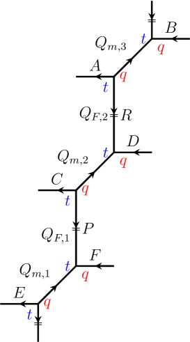
Figure 7: Three four-point amplitudes glued together vertically give the $A_{2}$ $q$-Selberg measure.

The Kähler parameters should be identified as follows:

$$\sqrt{\frac{q}{t}}Q_{m,1}=q^{-v}t^{-N_{1}},\qquad\sqrt{\frac{q}{t}}Q_{m,a}=t^{N_{a-1}-N_{a}}\quad\text{for}\quad a=2,\ldots,M-1,\qquad\sqrt{\frac{q}{t}}Q_{m,M}=t^{N_{M-1}},$$ (16)

$$Q_{F,a}=q^{u_{a}+\delta_{a,1}v+\frac{1}{2}}t^{-\frac{1}{2}}.$$ (17)

We skip the tedious technical details and give the final answer for the $A_{M-1}$ $q$-Selberg measure:

$$\mu_{A_{M-1}}(\vec{x}|\vec{u},v,\vec{N},q,t)=\Delta^{(q,t)}_{A_{M-1}}(x)\left(\prod_{a=1}^{M-1}\prod_{i=1}^{N_{a}}x_{a,i}^{u_{a}}\right)\prod_{i=1}^{N_{1}}\prod_{k=0}^{v-1}\left(1-q^{k}x_{1,i}\right),$$ (18)

where essential part of the measure is the $A_{M-1}$ $q$-Vandermonde determinant, which is given by

$$\Delta^{(q,t)}_{A_{M-1}}(\vec{x}_{\vec{R}})=\frac{\Delta^{(q,t)}(x_{R_{1}})\cdots\Delta^{(q,t)}(x_{R_{M-1}})}{\Delta^{(q,t)}(x_{R_{1}},x_{R_{2}})\cdots\Delta^{(q,t)}(x_{R_{M-2}},x_{R_{M-1}})}$$ (19)

where $x_{R_{a},i}=q^{R_{a,i}+1}t^{N_{a}-i}$, $\Delta^{(q,t)}(x)$ is given by Eq. (13) and

$$\Delta^{(q,t)}(x,y)=\prod_{k\geq 0}\prod_{i=1}^{N_{1}}\prod_{j=1}^{N_{2}}\frac{1-q^{k}\frac{x_{i}}{y_{j}}}{1-tq^{k}\frac{x_{i}}{y_{j}}}$$ (20)

Here $M-2$ denominators appear from $M$ four-point amplitudes like (10) and $M-1$ numerators arise from the identity (77) used to glue them together. Notice also that the vertex operator contribution $\prod(1-q^{k}x_{1,i})$ contains only the variables $x_{1,i}$ from the first integration contour. This is the general effect, seen in the $SU(N)$ versions of the AGT conjecture — the vertex operators, corresponding to Lagrangian quiver gauge theories are not general $W_{N}$ primary fields, but have dimension vector proportional to a single fundamental weight. We conclude that our gluing procedure correctly reproduces both the gauge theory results and the corresponding $W_{N}$ conformal blocks.

One can clearly sees the structure of the root system $A_{N-1}$ in the measure (19). Other classic root systems $\Phi$ can be obtained from orbifolding the toric CY, so that in general the $q$-Vandermonde is given by

$$\Delta^{(q,t)}_{\Phi}(\vec{x}_{\vec{R}})=\prod_{k=0}^{\beta-1}\left[\prod_{a<b}(\Delta^{(q,t)}(x_{a},x_{b}))^{A_{ab}}\prod_{a}\Delta^{(q,t)}(x_{a})\right],$$ (21)

where $A_{ab}$ is the Cartan matrix. The ADE case of this measure was derived in [48] and in [49].

2.2 $q$-deformed torus block

We next consider the four point amplitude with horizontal ends identified.

$$\parbox{85.35826pt}{\includegraphics[width=85.35826pt]{figures/toric-4pt-crop}}=\mathcal{N}q^{\frac{||R||^{2}-||P||^{2}}{2}}t^{\frac{||P^{\mathrm{T}}||^{2}-||R^{\mathrm{T}}||^{2}}{2}}M_{R}^{(q,t)}(t^{-\rho})M_{P^{\mathrm{T}}}^{(t,q)}(q^{-\rho})\times\\ \times\prod_{k\geq 1}\frac{G_{RP}^{(q,t)}\left(Q_{\tau}^{k-1}\sqrt{\frac{q}{t}}Q_{m}\right)G_{PR}^{(q,t)}\left(Q_{\tau}^{k}\sqrt{\frac{q}{t}}Q_{m}^{-1}\right)}{G_{PP}^{(q,t)}\left(Q_{\tau}^{k}\frac{q}{t}\right)G_{RR}^{(q,t)}\left(Q_{\tau}^{k}\right)},$$ (22)

where $Q_{\tau}=Q_{m}Q_{B}$ and the factor $\mathcal{N}$ is independent of the diagrams $R$, $P$. It is possible to express some infinite products in the r.h.s. of Eq. (22) in the form of theta-functions (see e.g. [50]), however we will not be concerned with modular properties and thus will not need this representation.

Let us describe the action of spectral duality for the compactified toric diagram. It is again the $\frac{\pi}{2}$ rotation of the diagram, and for the case of $t=q$ this is an explicit symmetry of the topological string formalism. Using this formalism one can again see that the poles in DF integral representation of the conformal block correspond to AGT-like decomposition of the spectral dual conformal block.

However, for $t\neq q$, refined vertex should be used. This vertex (1) is not rotation symmetric, and thus spectral duality requires a nontrivial change of basis of states of the topological string, which we briefly explained in the Introduction. This basis change from generalized Macdonald polynomials to a factorized basis (of Schur functions) is given by the nontrivial generalized Kostka functions. These matrix functions act in the tensor product of several Fock spaces and, therefore, depend on several Young diagrams. The number of diagrams is given by the number of parallel edges in the toric diagram. The case of compactified toric diagram corresponds to effectively infinite number of legs — one can understand the leg on a circle as an infinite array of “mirror images” in the uncompactified space.

Unfortunately, in this case the generalized Macdonald polynomials are in fact not yet known. Let us only notice that, unlike the uncompactified case, here the problem is nontrivial even for a single leg, i.e. a single Fock module, where the basis is labelled by a single Young diagram (though, of course depends on an extra parameter — the compactification radius).

2.2.1 Virasoro conformal block

Gluing two blocks (22) together we get the $q$-deformed Virasoro DF integral on torus, which is also known as the elliptic version of the $A_{1}$ Selberg integral:

$$\parbox{113.81102pt}{\includegraphics[width=113.81102pt]{figures/toric-vir-crop}}=\mathcal{N}\sum_{R}\left(Q_{F}\sqrt{\frac{t}{q}}\right)^{R}\prod_{k\geq 1}\frac{G_{R\varnothing}^{(q,t)}\left(Q_{\tau}^{k-1}\sqrt{\frac{q}{t}}Q_{m}\right)G_{\varnothing R}^{(q,t)}\left(Q_{\tau}^{k-1}\sqrt{\frac{q}{t}}Q_{m}\right)}{G_{RR}^{(q,t)}\left(Q_{\tau}^{k-1}\right)}\times\\ \times\prod_{k\geq 1}\frac{G_{\varnothing R}^{(q,t)}\left(Q_{\tau}^{k}\sqrt{\frac{q}{t}}Q_{m}^{-1}\right)G_{R\varnothing}^{(q,t)}\left(Q_{\tau}^{k}\sqrt{\frac{q}{t}}Q_{m}^{-1}\right)}{G_{RR}^{(q,t)}\left(\frac{q}{t}Q_{\tau}^{k}\right)}$$ (23)

where $Q_{\tau}=Q_{m}Q_{B}$. The sum over partitions in Eq. (23) can be recast into the contour integral of the elliptic Selberg form:

$$\oint d^{N}x\,\Delta^{(q,t,Q_{\tau})}(x)V_{u}(0,x)V_{N}(1,x),$$ (24)

where

$$\Delta^{(q,t,Q_{\tau})}(x)=\prod_{k\geq 1}\prod_{l\geq 0}\prod_{i\neq j}^{N}\frac{\left(1-q^{l}Q_{\tau}^{k-1}\frac{x_{i}}{x_{j}}\right)\left(1-q^{l}Q_{\tau}^{k}\frac{q}{t}\frac{x_{i}}{x_{j}}\right)}{\left(1-q^{l}Q_{\tau}^{k-1}t\frac{x_{i}}{x_{j}}\right)\left(1-q^{l}Q_{\tau}^{k}q\frac{x_{i}}{x_{j}}\right)},\qquad V_{u}(0,x)=\prod_{i=1}^{N}x_{i}^{u}$$ (25)

$$V_{v}(z,x)=\prod_{i=1}^{N}\prod_{k\geq 1}\prod_{l\geq 0}\frac{\left(1-q^{l}Q_{\tau}^{k-1}q^{-v}\frac{z}{x_{i}}\right)\left(1-q^{l}Q_{\tau}^{k}q^{-v}\frac{q}{t}\frac{z}{x_{i}}\right)}{\left(1-q^{l}Q_{\tau}^{k-1}\frac{z}{x_{i}}\right)\left(1-q^{l}Q_{\tau}^{k}\frac{q}{t}\frac{z}{x_{i}}\right)}$$ (26)

Here $t^{N}=\sqrt{\frac{q}{t}}Q_{m}$ and $q^{u}=Q_{F}\sqrt{\frac{t}{q}}$. Notice the symmetry between $q$ and $Q_{\tau}$ in the measure — this follows from the equivalence between the two compactified circles $S_{R_{5}}$ and $S_{R_{6}}$. This form of elliptic Selberg integral was used in [3] to formulate the elliptic version of the AGT correspondence. Notice that the dimension of the vertex operator $V_{N}(1,x)$ is not an independent variable, but is related to the number of integrations, and thus to the intermediate dimension in the toric conformal block.

2.2.2 $W_{M}$-algebra conformal block

The same procedure as in sec. 2.2.1 applies to the $W$-algebra case. We glue several compactified pieces like (22) together to obtain the toric diagram corresponding to the 5d $U(M)$ gauge theory with adjoint multiplet.

The corresponding $A$ elliptic Selberg measure is given by

$$\Delta^{(q,t,Q_{\tau})}_{A_{M-1}}(\vec{x})=\frac{\Delta^{(q,t,Q_{\tau})}(x_{1})\cdots\Delta^{(q,t,Q_{\tau})}(x_{M-1})}{\Delta^{(q,t,Q_{\tau})}(x_{1},x_{2})\cdots\Delta^{(q,t,Q_{\tau})}(x_{M-2},x_{M-1})},$$ (27)

where $\Delta^{q,t,Q_{\tau}}(x_{a})$ is given by Eq. (25) and

$$\Delta^{(q,t,Q_{\tau})}(x,y)=\prod_{k\geq 1}\prod_{i=1}^{N_{1}}\prod_{j=1}^{N_{2}}\frac{\left(1-q^{l}Q_{\tau}^{k-1}\frac{x_{i}}{y_{j}}\right)\left(1-q^{l}Q_{\tau}^{k}\frac{q}{t}\frac{y_{j}}{x_{i}}\right)}{\left(1-q^{l}Q_{\tau}^{k-1}t\frac{x_{i}}{y_{j}}\right)\left(1-q^{l}Q_{\tau}^{k}q\frac{y_{j}}{x_{i}}\right)}$$ (28)

Of course, the measure for any root system $\Phi$ can be obtained in a similar way:

$$\Delta_{\Phi}^{(q,t,Q_{\tau})}(\vec{x})=\left[\prod_{a=1}^{r}\Delta^{(q,t,Q_{\tau})}(x_{a})\right]\prod_{a<b}\Delta^{(q,t,Q_{\tau})}(x_{a},x_{b})^{A_{ab}},$$ (29)

where $A_{ab}$ is the Cartan matrix of the root system $\Phi$.

2.3 Affine spherical block

This case provides the vertex operator corresponding to the 6d gauge theory. It is very much analogous to the $W_{M}$ case considered above, however the root system is now not finite, but affine. The resulting algebra is doubly deformed — by $q$ and by an extra parameter $\tilde{t}$ related to the compactified sixth dimension. We start from the simplest example of $U(1)$ gauge theory and then generalize to higher rank groups. We also present an interesting generalization of the affine integrals in sec. 3.

2.3.1 $\widehat{\mathfrak{u}}(1)$ measure

The simplest example of 6d theory is the $U(1)$ linear quiver. It is built from the elementary block corresponding to the bifundamental field. In the topological string language this corresponds to a four point amplitude with vertical edges joined with each other.

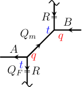
Figure 8: Four-point amplitude with vertical ends identified to obtain the $\widehat{\mathfrak{u}}_{1}$ $q$-Selberg measure.

The new feature appearing in this setting is that the width of the diagram featuring in the sum is not bounded, so that the number of $x_{i}$ variables in the corresponding integral becomes infinite:

$$\Delta^{(q,t,\tilde{t})}_{\widehat{\mathfrak{u}}_{1}}(x_{R})=\lim_{N\to\infty}\prod_{i\neq j}^{N}\prod_{k\geq 0}\frac{\left(1-q^{k}\frac{x_{R,i}}{x_{R,j}}\right)\left(1-t\tilde{t}q^{k}\frac{x_{R,i}}{x_{R,j}}\right)}{\left(1-tq^{k}\frac{x_{R,i}}{x_{R,j}}\right)\left(1-\tilde{t}q^{k}\frac{x_{R,i}}{x_{R,j}}\right)}$$ (30)

where $\tilde{t}=\sqrt{\frac{q}{t}}Q_{m}$. Notice the symmetry between $t$ and $\tilde{t}$, which is made explicit in the last expression. This should be compared to the analogous symmetry between $q$ and $Q_{\tau}$ in the toric measure (25). Of course, the two cases are related by the spectral duality, which partly explains the similarity. However, the exact relation between the two measures is nontrivial, since the sum over $R$ in Fig. 8 is over a different edge, than in Eq. (23). We will look more closely at the measure (30) in sec. 3.

2.3.2 $\widehat{A}_{M}$ measure

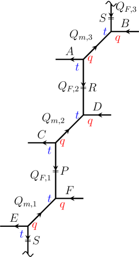
Figure 9: Three four-point amplitudes glued vertically in a cyclic fashion to obtain the $\widehat{A}_{2}$ $q$-Selberg measure.

The story is similar for several four-point amplitudes glued in a cyclic fashion in the vertical direction. The corresponding Vandermonde factor is

$$\Delta^{(q,t,\tilde{t})}_{\widehat{A}_{M-1}}(\vec{x}_{\vec{R}})=\lim_{N_{a}\to\infty}\frac{\prod_{a=1}^{M}\Delta^{(q,t)}(x_{R_{a}})}{\Delta^{(q,t)}(\tilde{t}x_{R_{1}},x_{R_{M}})\prod_{a=1}^{M-1}\Delta^{(q,t)}(x_{R_{a+1}},x_{R_{a}})}$$ (31)

where differences between $N_{a}$ are encoded by the Kähler parameters of the diagram: $t^{N_{a+1}-N_{a}}=\sqrt{\frac{q}{t}}Q_{m,a}$, $a=1,\ldots,M-1$, and $t^{N_{1}-N_{M}}\tilde{t}=\sqrt{\frac{q}{t}}Q_{m,M}$. Notice that the product corresponding to the additional affine root is distinguished, and contains an extra parameter $\tilde{t}$. Of course, one can rescale the variables $x_{R_{a}}$ so that the extra parameter appears in any other product. The other curious fact about the affine case is that the number of contours (and, thus, the number of Young diagrams in the sum over poles) in the $\widehat{A}_{M}$ measure is $M$, and not $M-1$ as in the $A_{M}$ case. This special point is closely related to the fact that the bosonization of the elliptic Virasoro algebra necessarily involves free fields of two sorts, whereas only one free field is needed in the rational and $q$-deformed cases.

2.4 Affine torus block

We proceed to describe the most advanced generalization, i.e. the double compactification of the diagram. It corresponds to the torus conformal block for the $W$-algebra of the affine algebra (also denoted by $W(\widehat{\mathfrak{g}})$).

2.4.1 Torus $\widehat{\mathfrak{u}}_{1}$ measure

Figure 10: Four-point amplitude with both vertical and horizontal ends identified to obtain the $\widehat{\mathfrak{u}}_{1}$ elliptic $q$-Selberg measure.

$$\Delta_{\widehat{\mathfrak{u}}_{1}}^{(q,t,\tilde{t},Q_{\tau})}(x)=\lim_{N\to\infty}\prod_{i\neq j}\prod_{k\geq 0}\prod_{l\geq 0}\frac{\left(1-Q_{\tau}^{k}q^{l}\frac{x_{i}}{x_{j}}\right)\left(1-Q_{\tau}^{k}q^{l}\frac{Q_{\tau}q}{t}\frac{x_{i}}{x_{j}}\right)}{\left(1-Q_{\tau}^{k}q^{l}t\frac{x_{i}}{x_{j}}\right)\left(1-Q_{\tau}^{k}q^{l}Q_{\tau}q\frac{x_{i}}{x_{j}}\right)}\frac{\left(1-Q_{\tau}^{k}q^{l}t\tilde{t}\frac{x_{i}}{x_{j}}\right)\left(1-Q_{\tau}^{k}q^{l}Q_{\tau}q\tilde{t}\frac{x_{i}}{x_{j}}\right)}{\left(1-Q_{\tau}^{k}q^{l}\tilde{t}\frac{x_{i}}{x_{j}}\right)\left(1-Q_{\tau}^{k}q^{l}\frac{Q_{\tau}q\tilde{t}}{t}\frac{x_{i}}{x_{j}}\right)}$$ (32)

This measure is symmetric with respect to the exchange of $q$ and $Q_{\tau}$, however the symmetry between $t$ and $\tilde{t}$ is lost.

2.4.2 Torus $\widehat{A}_{M}$ measure

We now have $M$ four-point amplitudes with edges totally contracted.

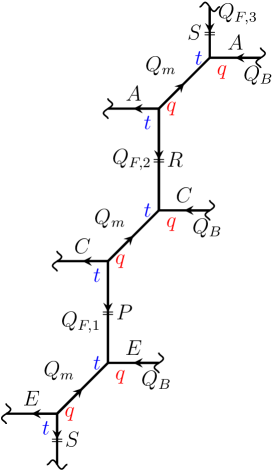
Figure 11: Three four-point amplitude with both vertical and horizontal ends identified to obtain the $\widehat{A}_{2}$ elliptic $q$-Selberg measure. Notice that $Q_{m,i}$ are now all the same, because of the constraints imposed by the closed hexagons formed by the identified edges.

The measure is a straightforward generalization of the $\widehat{\mathfrak{u}}_{1}$ measure:

$$\Delta^{(q,t,\tilde{t},Q_{\tau})}_{\widehat{A}_{M}}(\vec{x})=\frac{\prod_{a=1}^{M}\Delta^{(q,t,Q_{\tau})}(x_{(a)})}{\Delta^{(q,t,Q_{\tau})}(x_{(M)},\tilde{t}x_{(1)})\prod_{a=1}^{M-1}\Delta^{(q,t,Q_{\tau})}(x_{(a)},\tilde{t}x_{(a+1)})}$$ (33)

where

$$\Delta^{(q,t,Q_{\tau})}(x)=\lim_{N\to\infty}\prod_{i\neq j}\prod_{k\geq 0}\prod_{l\geq 0}\frac{\left(1-Q_{\tau}^{k}q^{l}\frac{x_{i}}{x_{j}}\right)\left(1-Q_{\tau}^{k}q^{l}\frac{Q_{\tau}q}{t}\frac{x_{i}}{x_{j}}\right)}{\left(1-Q_{\tau}^{k}q^{l}t\frac{x_{i}}{x_{j}}\right)\left(1-Q_{\tau}^{k}q^{l}Q_{\tau}q\frac{x_{i}}{x_{j}}\right)}$$ (34)

and

$$\Delta^{(q,t,Q_{\tau})}(x,y)=\lim_{N\to\infty}\prod_{i=1}^{N_{1}}\prod_{j=1}^{N_{2}}\prod_{k\geq 0}\prod_{l\geq 0}\frac{\left(1-Q_{\tau}^{k}q^{l}\frac{x_{i}}{y_{j}}\right)\left(1-Q_{\tau}^{k}q^{l}\frac{Q_{\tau}q}{t}\frac{y_{j}}{x_{i}}\right)}{\left(1-Q_{\tau}^{k}q^{l}t\frac{x_{i}}{y_{j}}\right)\left(1-Q_{\tau}^{k}q^{l}Q_{\tau}q\frac{y_{j}}{x_{i}}\right)}$$ (35)

3 6d theory, affine Selberg integral and index vertex

In this section we investigate in more detail the affine Selberg integrals first described in sec. 2.3 and point out an interesting natural generalization of them.

We start with the simplest example and evaluate the partition function of the trivial 6d theory with “zero” gauge group and only one free multiplet using refined topological string. The corresponding toric diagram is compactified along the preferred direction, as shown on Fig. 12.

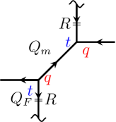
Figure 12: Compactified resolved conifold corresponding to free hypermultiplet in 6d or (in the spectral dual frame) to 5d $U(1)$ theory with adjoint hypermultiplet.

It is straightforward to obtain the (spectral dual) partition function, which is given by the Nekrasov formula, i.e. the sum over Young diagrams:

$$Z^{\text{5d, adj}}_{U(1)}=\sum_{R}\left(\sqrt{\frac{t}{q}}Q_{F}\right)^{|R|}\frac{G_{RR}^{(q,t)}\left(\sqrt{\frac{q}{t}}Q_{m}\right)}{G_{RR}^{(q,t)}(1)}.$$ (36)

Using the standard identities we can rewrite this sum over diagrams as a contour integral of $q$-Selberg type:

$$Z^{\text{5d, adj}}_{U(1)}=\lim_{Q\to 1}\lim_{N\to\infty}\mathcal{N}^{-1}\oint_{\gamma}d^{N}x\prod_{i=1}^{N}x_{i}^{u}\prod_{k\geq 0}\left[\prod_{i\neq j}\frac{\left(1-q^{k}\frac{x_{i}}{x_{j}}\right)\left(1-t\tilde{t}q^{k}\frac{x_{i}}{x_{j}}\right)}{\left(1-tq^{k}\frac{x_{i}}{x_{j}}\right)\left(1-\tilde{t}q^{k}\frac{x_{i}}{x_{j}}\right)}\prod_{i=1}^{N}\frac{1-\frac{Qq^{k}z_{1}}{x_{i}}}{1-\frac{q^{k}z_{1}}{x_{i}}}\right]$$ (37)

where $\tilde{t}=\sqrt{\frac{q}{t}}Q_{m}$, $q^{u}=\sqrt{\frac{t}{q}}Q_{F}$ and $\mathcal{N}$ is the normalization constant. The poles are enumerated by Young diagrams $R$ and are located at points

$$x_{R,i}=z_{1}q^{R_{i}}t^{N-i}.$$ (38)

The integral (37) differs from the ordinary $q$-Selberg integral from sec. 2.1.1 in several respects:

1. The measure is of affine Selberg type, more precisely of type $\widehat{\mathfrak{u}}_{1}$. This is in close analogy with the $A_{n}$ Selberg measure (see sec. 2.1.2), though the factor corresponding to the imaginary root contains extra $\tilde{t}$.

2. The integration measure in Eq. (37) is explicitly symmetric between $t$ and $\tilde{t}$. This symmetry is completely unexpected from the point of view of the topological strings: $\tilde{t}$ in this framework represents the Kähler parameter of the resolved conifold while $t$ is the refinement parameter. Neither is this symmetry obvious from the corresponding 5d gauge theory: here $\tilde{t}$ is the mass of the adjoint multiplet and $t$ is one of the equivariant parameters.

3. The curious feature of the integral (37) is the appearance of the special contour $\gamma$, which encircles only pole of the form $x_{i}=z_{1}q^{k}t^{l}$ with $k,l\geq 0$ and excludes the poles $x_{i}=z_{1}q^{k}t^{l}\tilde{t}^{m}$ with nonzero $m$. This choice of contour explicitly breaks the symmetry between $t$ and $\tilde{t}$ in the measure, so that the whole partition function is no longer symmetric. This can also be seen from the explicit infinite product formula for the partition function (36), which has no symmetry between $\sqrt{\frac{q}{t}}Q_{m}$ and $t$.

4. The adjoint Nekrasov factors (36) are non-vanishing for Young diagrams of arbitrary width. Thus, the number of integrations in (37) is also infinite.

5. We insert an additional vertex operator $V_{Q}(z_{1})=\prod_{i=1}^{N}\frac{1-\frac{Qq^{k}z_{1}}{x_{i}}}{1-\frac{q^{k}z_{1}}{x_{i}}}$ at $z_{1}$ to produce the poles of the necessary form (38). We then take the limit $Q\to 1$ so that the extra factors cancel. One can naively think that the integral vanishes in this limit, since the poles in the denominator cancel with the zeroes of the numerator. However, we are in fact interested in the ratio of the residues at the points (38). More concretely, one sets $\mathcal{N}=\mathop{\mathrm{Res}}\limits_{x_{\varnothing,i}}\mu(x)$, where $\mu(x)$ is the integrand, so that the sum over residues starts from the identity and is finite for $Q\to 1$. The value of the integral in this limit of course does not depend on the position $z_{1}$ of the vertex operator. We, therefore, view the additional factors in (37) as a regularization.

In the next section we modify the integral (37) to include all the poles and find that this is exactly the equivariant instanton partition function of the 6d $(1,1)$ gauge theory on $\mathbb{R}^{6}$.

3.1 Extending the contour

Let us consider the following integral [20]

$$\boxed{Z_{\mathrm{ext}}^{U(1)}=\lim_{Q\to 1}\lim_{N\to\infty}\mathcal{N}^{-1}\oint\limits_{|x_{i}|=|z_{1}|+\epsilon}d^{N}x\prod_{i=1}^{N}x_{i}^{u}\prod_{k\geq 0}\left[\prod_{i\neq j}\frac{\left(1-q^{k}\frac{x_{i}}{x_{j}}\right)\left(1-t\tilde{t}q^{k}\frac{x_{i}}{x_{j}}\right)}{\left(1-tq^{k}\frac{x_{i}}{x_{j}}\right)\left(1-\tilde{t}q^{k}\frac{x_{i}}{x_{j}}\right)}\prod_{i=1}^{N}\frac{1-\frac{Qq^{k}z_{1}}{x_{i}}}{1-\frac{q^{k}z_{1}}{x_{i}}}\right]}$$ (39)

where we assume $|q|<1$, $|t|>1$, $|\tilde{t}|>1$ and $\mathcal{N}=\mathop{\mathrm{Res}}\limits_{x_{\varnothing,i}}\mu(x)$. Notice the main difference with (37) — the contour now encircles all the poles at $x_{i}=z_{1}q^{k}t^{-l}\tilde{t}^{-m}$ with $k$, $l$, $m$ nonnegative.

Enumerating the poles.

Consider first the terms with $k=0$ in the integrand of Eq. (39). Then for finite $N$ the situation is completely analogous to the LMNS integrals for $U(1)$ gauge theory [43] (we will elaborate on this analogy in sec. 3.4). One can see that one of the variables $x_{i}$ should pick up a pole coming from the vertex operator. The whole integrand is symmetric in $x_{i}$, so we can think that this is the first variable, i.e. $x_{1}=z_{1}$. Suppose then, that we have already performed the first $l<N$ integrals and have picked the poles, at $x_{i}=z_{1}t^{1-n}\tilde{t}^{1-m}$, where $(n,m)\in Y^{\prime}\subset Y$. Then the next integration produces the following poles:

$$x_{l}=z_{1}t^{1-n\mp 1}\tilde{t}^{1-m},\quad x_{l}=z_{1}t^{1-n}\tilde{t}^{1-m\mp 1},\quad(n,m)\in Y^{\prime}$$ (40)

There are also zeroes:

$$x_{l}=z_{1}t^{1-n}\tilde{t}^{1-m}\text{ (double)},\quad x_{l}=z_{1}t^{-n}\tilde{t}^{-m},\quad x_{l}=z_{1}t^{2-n}\tilde{t}^{2-m},\quad(n,m)\in Y^{\prime}$$ (41)

Some poles are canceled by zeroes, and only small portion of them survives. In particular, if a point lies inside of $Y^{\prime}$ and not on the boundary of $Y^{\prime}$, then there are exactly 4 poles and 4 zeroes which cancel them. So, there is no pole to pick strictly inside $Y^{\prime}$. On the boundary the situation is a bit more subtle, and there are corner contributions, recursion relations, etc. — for details see [51]. However, when the dust settles one gets the simple recipe, i.e. that each successive integration adds a box so that the whole set of poles remains a Young diagram. All the poles thus organize themselves into a Young diagram $Y$ with $N$ boxes:

$$x_{i,j}=z_{1}t^{1-i}\tilde{t}^{1-j},\quad(i,j)\in Y.$$ (42)

The terms with $k>0$ have a simple effect — each pole $x_{i,j}$ is now shifted by $q^{k}$ with respect to the poles at $x_{i+1,j}$ or $x_{i,j+1}$. Thus, the poles are now labelled by a plane partition (3d Young diagram) $\pi$ with floor area $N$, so that $x_{i,j}=z_{1}q^{\pi_{i,j}-1}t^{1-i}\tilde{t}^{1-j}$.

For infinite $N$ a slightly different picture is more convenient. Let us demolish the “stylobate” of $\pi$ – i.e. reduce the height of each column by one. The resulting plane partition has floor area less or equal to $N$ and will be denoted by $\tilde{\pi}$, so that $\tilde{\pi}_{i,j}=\pi_{i,j}-1$.

Computing the residues.

Let us now compute the residues at the poles. More concretely, since the normalization constant is the contribution of the pole corresponding to the empty diagram, we are actually computing the ratio of the residues (the same trick was used in [13]):

$$Z_{\mathrm{ext}}^{U(1)}=\sum_{\tilde{\pi}}\frac{\mathop{\mathrm{Res}}\limits_{x_{\tilde{\pi}}}\mu(x)}{\mathop{\mathrm{Res}}\limits_{x_{\varnothing}}\mu(x)}=\sum_{\pi}\frac{\mu(x_{\pi})}{\mu(x_{\varnothing})}$$ (43)

We find that the residues have the following plethystic form:

$$\frac{\mu(x_{\pi})}{\mu(x_{\varnothing})}=q^{u|\tilde{\pi}|}\exp\left\{-\sum_{n\geq 1}\frac{1}{n}\left[\frac{(1-t^{n})(1-\tilde{t}^{n})}{1-q^{n}}\left(p_{n}(x_{\tilde{\pi}})p_{-n}(x_{\tilde{\pi}})-p_{n}(x_{\varnothing})p_{-n}(x_{\varnothing})\right)\right]\right\}.$$ (44)

where $p_{n}(x)$ are power sum symmetric functions. We can take the limit $N\to\infty$ in each term, and the power sums become

$$p_{n}(x_{\tilde{\pi}})=\sum_{i,j\geq 1}^{\infty}q^{n\tilde{\pi}_{i,j}}t^{n(1-i)}\tilde{t}^{n(1-j)}=\frac{1}{(1-t^{-n})(1-\tilde{t}^{-n})}+(q^{n}-1)\sum_{(i,j,k)\in\pi}q^{n(k-1)}t^{n(1-i)}\tilde{t}^{n(1-j)}=\\ =\frac{1}{(1-t^{-n})(1-\tilde{t}^{-n})}\left[1-(1-q^{n})(1-t^{-n})(1-\tilde{t}^{-n})\mathop{\mathrm{ch}}\nolimits_{\tilde{\pi}}(t^{-n},\tilde{t}^{-n},q^{n})\right],$$ (45)

where the $\mathop{\mathrm{ch}}\nolimits_{\tilde{\pi}}(q_{1},q_{2},q_{3})=\sum_{(i,j,k)\in\tilde{\pi}}q_{1}^{i-1}q_{2}^{j-1}q_{3}^{k-1}$. Finally, the value of the residues is given by

$$\frac{\mu(x_{\tilde{\pi}})}{\mu(x_{\varnothing})}=q^{u|\tilde{\pi}|}\exp\left\{-\sum_{n\geq 1}\frac{1}{n}\frac{E_{\tilde{\pi}}(t^{-n},\tilde{t}^{-n},q^{n})E_{\tilde{\pi}}(t^{n},\tilde{t}^{n},q^{-n})-1}{(1-t^{-n})(1-\tilde{t}^{-n})(1-q^{n})}\right\},$$ (46)

where $E_{\tilde{\pi}}(q_{1},q_{2},q_{3})=1-(1-q_{1})(1-q_{2})(1-q_{3})\mathop{\mathrm{ch}}\nolimits_{\tilde{\pi}}(q_{1},q_{2},q_{3})$. In s. 3 we have found an unexpected symmetry between $t$ and $\tilde{t}$ in the integration measure. However, the choice of the special contour $\gamma$ did not respect this symmetry. Choosing the contour $|x|=|z_{1}|+\epsilon$ we not only restore the symmetry $t\leftrightarrow\tilde{t}$, but also get a free bonus. The partition function (46) is actually completely symmetric in $t^{-1}$, $\tilde{t}^{-1}$ and $q$. This is part of our motivation for extending the integration contour. Topological string theory does not give a clue about the origin of this extra symmetry. In the next section we will argue that it can be understood from the six-dimensional point of view. More concretely, we will show that Eq. (46) exactly reproduces the sum over fixed points in the instanton moduli space of the 6d $\mathcal{N}=(1,1)$ $U(1)$ gauge theory.

3.2 6d $\mathcal{N}=(1,1)$ $U(1)$ theory and the index vertex

The $\mathcal{N}=(1,1)$ gauge theory has the maximal possible supersymmetry in six dimensions. It can be straight-forwardly obtained from dimensional reduction of 10d $\mathcal{N}=1$ gauge theory. In flat Euclidean space the supersymmetry can be equivariantly twisted using the maximal torus of isometries of $\mathbb{R}^{6}$, i.e. $U(1)^{3}$. The equivariant partition function, therefore, depends on three equivariant parameters $q_{1,2,3}=e^{\epsilon_{1,2,3}}$. The equivariant integrals over the $Q$-closed field configurations localize on the fixed points, which are labelled by plane partitions, so that the instanton partition function is given by the sum over fixed points each taken with its equivariant index [34], [52]

$$Z^{\mathrm{6d}(1,1)U(1)}_{\mathrm{inst}}=\sum_{\pi}\Lambda^{|\pi|}\mathrm{Ind}_{\pi}(q_{1},q_{2},q_{3}),$$ (47)

where $\Lambda$ is the coupling constant. The index of each fixed point is given by the product of $U(1)^{3}$ weights:

$$\mathrm{Ind}_{\pi}(q_{1},q_{2},q_{3})=\prod_{i}(1-e^{w_{i}(q,\pi)})^{\pm 1}$$ (48)

It is convenient to write the weights in the plethystic form:

$$\mathrm{Ind}_{\pi}(q_{1},q_{2},q_{3})=\exp\left[\sum_{n\geq 1}\frac{1}{n}\mathop{\mathrm{ch}}\nolimits_{T\pi}(q_{1}^{n},q_{2}^{n},q_{3}^{n})\right]$$ (49)

where the character of the tangent space to the fixed point is given by

$$\mathop{\mathrm{ch}}\nolimits_{T\pi}(q_{1},q_{2},q_{3})=\sum_{i}\mp e^{w_{i}(q,\pi)}$$ (50)

These characters have been found in [35] and are given by

$$\mathop{\mathrm{ch}}\nolimits_{T\pi}(q_{1},q_{2},q_{3})=\frac{1-E_{\pi}(q_{1},q_{2},q_{3})E_{\pi}(q_{1}^{-1},q_{2}^{-1},q_{3}^{-1})}{(1-q_{1}^{-1})(1-q_{2}^{-1})(1-q_{3}^{-1})}.$$ (51)

One immediately sees that this sum over fixed points is exactly the same as the sum over poles in Eq. (46) provided one makes the following identifications:

$$\boxed{\begin{array}[]{rcl}q_{1}&=&t^{-1},\\ q_{2}&=&\tilde{t}^{-1}=\sqrt{\frac{q}{t}}Q_{m},\\ q_{3}&=&q,\\ \Lambda&=&q^{u}=\sqrt{\frac{t}{q}}Q_{F}.\end{array}}$$ (52)

At this point several remarks are in order.

1. Partition function, similar to (47) was used in [34] to find the partition function of topological strings on the $\mathbb{C}^{3}$ patch of a toric CY manifold. The main difference from (47) was that the plane partitions were allowed to have infinite “legs” along the three coordinate axes, so that the resulting vertex depended on the three Young diagrams in the asymptotics.

2. Using the map (52) one can understand the remarkable symmetry between $t$, $\tilde{t}$ and $q$ in the enlarged integral as the symmetry between three equivariant parameters in $\mathbb{R}^{6}$, and eventually relate it to the action of the Weyl group of $SO(6)$.

3.3 Generalizing to $U(N)$/quiver of $U(1)$ groups

Generalization to linear quiver of $U(1)$ groups in 6d or equivalently to 5d $U(N)$ gauge theory is straightforward. We consider a stack of $N$ compactified resolved conifolds as shown on Fig. 13.

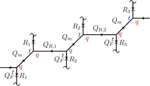
Figure 13: Stack of compactified resolved conifolds corresponding to 5d $U(3)$ theory with adjoint hypermultiplet.

The partition function is just 5d $U(N)$ Nekrasov function with adjoint multiplet. It has an integral representation quite similar to (37), the only difference is that there are $N$ vertex operator insertions at points $z_{1}$,…, $z_{N}$:

$$Z^{\text{5d, adj}}_{U(N)}=\lim_{Q_{a}\to 1}\lim_{M\to\infty}\mathcal{M}^{-1}\oint_{\gamma}d^{M}x\prod_{i=1}^{M}x_{i}^{u}\prod_{k\geq 0}\left[\prod_{i\neq j}\frac{\left(1-q^{k}\frac{x_{i}}{x_{j}}\right)\left(1-t\tilde{t}q^{k}\frac{x_{i}}{x_{j}}\right)}{\left(1-tq^{k}\frac{x_{i}}{x_{j}}\right)\left(1-\tilde{t}q^{k}\frac{x_{i}}{x_{j}}\right)}\prod_{a=1}^{N}\prod_{i=1}^{M}\frac{1-\frac{Q_{a}q^{k}z_{1}}{x_{i}}}{1-\frac{q^{k}z_{a}}{x_{i}}}\right]$$ (53)

The poles of the integral are now enumerated not by one partition, but by an $N$-tuple of partitions $\vec{R}=(R_{1},\ldots,R_{N})$, so that $x_{\vec{R}}=\tilde{z}_{a}q^{R_{a,i}}t^{1-i}$, where $\tilde{z}_{a}=z_{a}t^{N_{a}-1}$.

Just as in the $U(1)$ case, the contour $\gamma$ can be extended to encircle the additional poles, so that the whole partition function is the sum over $N$-tuples of plane partitions, $\vec{\pi}=(\pi_{1},\ldots,\pi_{N})$, and $x_{\vec{\pi}}=\tilde{z}_{a}q^{\pi_{a,i,j}}t^{1-i}\tilde{t}^{1-j}$. Moreover, the sum over residues exactly reproduces the localization formula for the 6d $\mathcal{N}=(1,1)$ $U(N)$ theory. For the (scaled) sum over residues we have:

$$Z_{\mathrm{ext}}^{U(N)}=\sum_{\vec{\pi}}\frac{\mathop{\mathrm{Res}}\limits_{x_{\vec{\pi}}}\mu(x)}{\mathop{\mathrm{Res}}\limits_{x_{\varnothing}}\mu(x)}=\sum_{\vec{\pi}}\frac{\mu(x_{\vec{\pi}})}{\mu(x_{\varnothing})}=\\ =\sum_{\vec{\pi}}q^{u|\vec{\pi}|}\exp\left\{-\sum_{n\geq 1}\frac{1}{n}\left[\frac{(1-t^{n})(1-\tilde{t}^{n})}{1-q^{n}}\left(p_{n}(x_{\vec{\pi}})p_{-n}(x_{\vec{\pi}})-p_{n}(x_{\varnothing})p_{-n}(x_{\varnothing})\right)\right]\right\}=\\ =\sum_{\vec{\pi}}q^{u|\vec{\pi}|}\exp\left\{-\sum_{n\geq 1}\frac{1}{n}\left[\frac{(1-t^{n})(1-\tilde{t}^{n})}{1-q^{n}}\sum_{a,b=1}^{N}z_{a}^{n}z_{b}^{-n}\left(p_{n}(x_{\pi_{a}})p_{-n}(x_{\pi_{b}})-p_{n}(x_{\varnothing})p_{-n}(x_{\varnothing})\right)\right]\right\}$$ (54)

Whereas the localization in the gauge theory looks similar to (47):

$$Z_{\mathrm{inst}}^{6d(1,1)U(N)}=\sum_{\vec{\pi}}\Lambda^{|\vec{\pi}|}\mathrm{Ind}_{\vec{\pi}}(q_{1},q_{2},q_{3}),$$ (55)

except the index now depends on $N$-tuple of plane partitions and $N$ Coulomb moduli of the theory:

$$\mathrm{Ind}_{\vec{\pi}}(q_{1},q_{2},q_{3})=\exp\left\{-\sum_{n\geq 1}\frac{1}{n}\frac{W(\vec{a}^{n},\vec{q}^{n})W(\vec{a}^{-n},\vec{q}^{-n})-E_{\vec{\pi}}(\vec{a}^{n},\vec{q}^{n})E_{\vec{\pi}}(\vec{a}^{-n},\vec{q}^{-n})}{(1-q_{1}^{-n})(1-q_{2}^{-n})(1-q_{3}^{-n})}\right\},$$ (56)

where

$$W(\vec{a},\vec{q})=\sum_{p=1}^{N}a_{p},\qquad E(\vec{a},\vec{q})=\sum_{p=1}^{N}\sum_{(i,j,k)\in\pi_{a}}a_{p}q_{1}^{i-1}q_{2}^{j-1}q_{3}^{k-1}$$ (57)

Notice, that for $N=1$ the dependence of the index on $a_{p}$ drops out, as it should (there are no Coulomb moduli in the abelian theory). Partition functions (54) and (55) manifestly coincide if we make the following identification of the gauge theory and topological string parameters:

$$\boxed{\begin{array}[]{rcl}q_{1}&=&t^{-1}\\ q_{2}&=&\tilde{t}^{-1}=\sqrt{\frac{q}{t}}Q_{m}\\ q_{3}&=&q\\ \Lambda&=&q^{u}=\sqrt{\frac{t}{q}}Q_{F}\\ a_{p}&=&\tilde{z}_{p}\end{array}}$$ (58)

Notice that the extended integral in the $U(N)$ case is still symmetric in $q$, $t^{-1}$ and $\tilde{t}^{-1}$.

3.4 AGT: LMNS integral from the extended DF integral

The LMNS integrals and DF integrals describe respectively the instanton partition functions and conformal blocks. Their equivalence is known as AGT duality and it is usually seen as a non-trivial integral transform of the Habbard-Stratonovich type [45]. In [20], we suggested that it can actually be raised to an explicit symmetry. Namely, our extended “six-dimensional” integral is a certain generalization of both integrals, which can be turned into either the $q$-deformed version of the DF integral or the 5d LMNS integral in suitable limits. These two limits are given by $\tilde{t}\to 0$ and $q\to 0$ respectively, and the resulting expressions are related by transformations $t^{-1}\leftrightarrow\tilde{t}^{-1}\leftrightarrow q$. This is an exact and explicit symmetry of the integral. This limiting procedure straightforwardly generalizes to $U(N)$ theory. Since the initial extended integral is still symmetric in the three equivariant parameters, DF and LMNS representations are exactly equivalent.

One can go further and study the 4d limit of the gauge theory. In this case $q$-deformed DF integral turns into the ordinary DF or beta-ensemble integral, and 5d LMNS integral reduces to the ordinary LMNS one. However, at this level the symmetry is no longer explicit and looks almost like a miracle, if one does not know that the integrals came from an explicitly symmetric 6d expression.

4 Spectral dualities and elliptic integrable systems

4.1 Generalities

According to [21], the hierarchy of physical theories associated with brane configurations in string and low-energy Yang-Mills models actually begins with much simpler integrable systems, and Seiberg-Witten theory is exactly the one, which captures the information available at this level of description. Moreover, the Nekrasov deformation of Seiberg-Witten theory corresponds to a quantization of these systems [32], or, more precisely, a lifting from quasiclassical to full-fledged $\tau$-function theory, what, within the integrable theory context, is a general straightforward procedure, which does not require any additional information.

This circle of ideas was further developed and exploited in numerous works. It is now well known that, within this context, the 5d gauge theory with adjoint hypermultiplet corresponds to the elliptic Ruijsenaars system [29], the 6d linear quiver theory gives the XYZ spin chain [27] and the 6d gauge theory with adjoint matter is described by the double elliptic integrable system [31]. In other words, for generic toric diagrams, which we consider in this paper, we have the following table:

	Dimension	Sphere	Torus
algebra	4d	XXX chain	Elliptic Calogero
$q$-deformed algebra	5d	XXZ chain	Elliptic Ruijsenaars
doubly-deformed algebra	6d	XYZ chain	Double elliptic

All these systems should be related by various dualities, of which the most non-trivial are spectral dualities, interchanging vertical and horizontal directions in toric diagrams. They make XYZ spin chain equivalent to the Ruijsenaars system and different double elliptic systems are also equivalent. In the integrable system context, this equivalence was first realized by K.Hasegawa [53] (in fact, in some part by E.Sklyanin [54]). We describe it briefly in this section, postponing the details until a separate paper [10].

Let us start simply by counting the parameters of the spectral dual gauge theories.

$SU(N)$ theory with fundamental matter in 6d has the following parameters: Coulomb moduli $a_{i}$, $i=1,\ldots,N-1$, masses of the fundamental hypermultiplets $m_{i}^{\pm}$, $i=1,\ldots,N$, the coupling constant $\Lambda$ and the two radii of the compactified dimensions $R_{5}$ and $R_{6}$. There is also one feature unique to 6d theories: the masses cannot all be set independently, but there is one condition on them. This makes the total number of parameters $3N+1$.

$SU(2)^{N}$ necklace quiver theory in 5d has the following parameters parameters: Coulomb moduli $\widetilde{a}_{i}$, $i=1,\ldots,N$, masses of the bifundamentals $\widetilde{m}_{i}$, $i=1,\ldots,N$, coupling constants $\widetilde{\Lambda}_{i}=1,\ldots,N$, and the radius of the fifth dimension $R_{5}$. In total one gets $3N+1$ parameters.

This counting can also be seen on the toric diagram. We consider the example of $SU(2)^{4}$:

The amplitude depends on $5\times 4=20$ Kähler parameters written explicitly on the diagram and also on the radius $R_{5}$ of the M-theory circle. Each hexagon on the diagram enforces a pair of constraints on the Kähler parameters of its edges:

$$Q_{F,i}\widetilde{Q}_{i}=Q_{F,i+1}Q_{i+1},\qquad i=1,\dots,4,$$ (59)

$$Q_{B,i}Q_{i+1}=\widetilde{Q}_{i}\widetilde{Q}_{B,i},\qquad i=1,\ldots 4.$$ (60)

where we set $Q_{F,i+4}=Q_{F,i}$, etc. In total we get $5\times 4-2\times 4=3\times 4=12$ independent Kähler parameters and $R_{5}$, which agrees with the gauge theory counting, which also gives $3N+1=3\times 4+1=13$.

4.2 XYZ chain

$SU(N)$ gauge theory with $2N$ fundamental hypermultiplets in 6d corresponds [27] to the Sklyanin $N$-site $U_{q,t}(\mathfrak{gl}_{2})$ XYZ spin chain [54]. The transfer matrix of the spin chain is written in terms of Lax matrices, residing on each site of the chain with the corresponding inhomogeneity $\xi_{i}$:

$$T(\xi)=L^{(N)}(\xi-\xi_{N})\ldots L^{(1)}(\xi-\xi_{1}),$$ (61)

where

$$L(\xi)=S^{0}\cdot{\bf 1}+i\sum_{a=1}^{3}W_{a}(\xi)S^{a}\sigma_{a}$$ (62)

$\sigma_{a}$ are the Pauli matrices, and

$$W_{a}(\xi)=\sqrt{e_{a}-\wp\left({\xi}|\tau\right)}=i\frac{\theta^{\prime}_{\ast}(0)\theta_{a+1}\left({\xi}\right)}{\theta_{a+1}(0)\theta_{*}(\xi)}$$ (63)

where $\theta_{a}(x)$ is the standard Jacobi $\theta$-function and $e_{i}$ are values of the Weierstrass function $\wp(\xi)$ at the half-periods. The dynamical variables $S^{0},S^{a}$ form the (classical) Sklyanin algebra [54]:

$$\left\{S^{a},S^{0}\right\}=-i\left(e_{b}-e_{c}\right)S^{b}S^{c}\ \ \ \ \ \ \ \left\{S^{a},S^{b}\right\}=-iS^{0}S^{c}$$ (64)

with the obvious notation: $abc$ is the triple $123$ or its cyclic permutations.

For this $U_{q,t}(\mathfrak{gl}_{2})$ chain there are two Casimir operators, i.e. one degree of freedom remaining per site, which means that there are totally $N$ action variables, which correspond to $N$ Coulomb moduli $a_{i}$. However, one can consider vanishing the full momentum of the system (which corresponds to removing the $U(1)$-factor in the gauge theory), in this way, we are left with $N-1$ Coulomb moduli. The Casimirs and inhomogeneities are combined into $2N$ parameters of the fundamental hypermultiplet masses [27, (4.14)-(4.15)]. In fact, there is a restriction imposed on the sum of all masses [27], thus, there are $2N-1$ parameters. This matches the counting of degrees of freedom above.

The 5d and 4d reductions of this theory is described by the XXZ and XXX chain respectively.

4.3 Elliptic spin Ruijsenaars system

The $SU(N)$ gauge theory with the adjoint hypermultiplet in 5d corresponds [29] to the elliptic Ruijsenaars system [55] given by the Lax operator

$$L_{ij}(\xi)=c(\xi|\epsilon)e^{p_{i}}\prod_{k\neq i}\sqrt{\wp(q_{ik})-\wp(\epsilon)}{F(q_{ij}|\xi)\over F(q_{ij}|\epsilon)}\ \ \ \ \ \ \ \ F(q|\xi)={\theta(q+\xi)\theta^{\prime}(0)\over\theta(q)\theta(\xi)}$$ (65)

where $c(\xi|\epsilon)$ is a normalization factor which has to be chosen in a convenient way.

In order to extend this theory to the product of gauge groups, one first has to consider the spin elliptic Ruijsenaars system [56]. Then, the corresponding Lax operator is just

$$L_{ij}(\xi)\sim S_{ij}e^{p_{i}}\prod_{k\neq i}\sqrt{\wp(q_{ik})-\wp(\epsilon)}{F(q_{ij}|\xi)\over F(q_{ij}|\epsilon)}$$ (66)

with more dynamical variables: spins $S_{ij}$.

The next step is to extend it further to multi-point system. The Lax operator in this case becomes much more involved and so does the Poisson bracket of the spin variables $S^{a}_{ij}$ [10]. For the sake of simplicity, we write down here only the 4d case, when the system is multi-point Calogero system, and the formulas are much more compact, while the 5d formulas can be found in [10]. In the 4d case, the gauge theory has the gauge group $U(1)\times SU(N)^{k}$ and contains $k$ matter bifundamentals [38]. On the integrable side, the multi-point spin Calogero system is described by the Lax operator given on a torus with $k$ marked points $w_{a}$, [57]:

$$L_{ij}(\xi)=\delta_{ij}\left(p_{i}+\sum_{a}S^{a}_{ii}\zeta(\xi-w_{a})\right)+(1-\delta_{ij})\sum_{a}S_{ij}^{a}F(q_{ij}|\xi-w_{a})$$ (67)

where the spin variables satisfy the Poisson bracket

$$\{S_{ij}^{a},S_{kl}^{b}\}=\delta_{ab}\left(S_{il}^{a}\delta_{jk}-S^{a}_{jk}\delta_{il}\right)$$ (68)

and there is an additional constraint

$$\sum_{a}S^{a}_{ii}=0$$ (69)

The Poisson bracket is non-degenerate upon reducing the spin matrices to the orbits of $\mathfrak{gl}_{N}$. Thus, the system is characterized by the three integers: the number of particles $N$, the number of marked points $k$ and the parameter of the orbit $l$.

4.4 Spectral duality

The spectral duality, which we mentioned in ss.1.1 and 4.1, connects the Seiberg-Witten theories in 6d and 5d gauge theories. At the level of integrable systems, it was established by K.Hasegawa [53] (see also a trigonometric version of the correspondence in [58]) and claims an equivalence of the elliptic multi-point spin Ruijsenaars system given by $(N,k,l)$ and the elliptic spin chain on $k$ sites, given by the $l$-orbit of the Sklyanin- Odesskii-Feigin $\mathfrak{gl}_{N}$ [59]. In the particular case of $l=1$ (the orbit of minimal dimension), one obtains the duality between $SU(N)^{k}$ theory with fundamental matter in 6d and $SU(k+1)^{N}$ necklace quiver theory in 5d. Since this is a subject of its own value, we discuss implications of this Hasegawa correspondence between integrable systems in some more detail in a separate paper [10].

This duality can be lifted to the 6d theories with adjoint matter, which are described by the double elliptic integrable systems [31]. These systems have not been studied in full yet, because of a very involved structure (see [60] for some new advances). As usual, they appear from explicit expressions for partition function in section 3 in quasiclassical limit $\epsilon_{1}\sim\epsilon_{2}\longrightarrow 0$, while in Nekrasov-Shatashvili limit [32] (when only $\epsilon_{2}\longrightarrow\infty$) we get their straightforward quantization, when the spectral curve is substituted by a Baxter equation (quantum spectral curve). Analysis of these limits could help to describe the full integrable double elliptic system.

5 Conclusion

In this paper, we attempted to describe the Seiberg-Witten/Nekrasov theory for the most general model associated with an arbitrary $(p,q)$-web toric diagram (the tropical limit of the spectral curve). In the gauge theory language, this corresponds to 6d theory, in the integrable system language to the double elliptic system. We explained that the recent advances in the theories of Dotsenko-Fateev integrals and topological integrals provide a straightforward dictionary for conversion between the pictorial language of toric diagrams (spectral curves) and the Young-diagram expansions for the Nekrasov functions, and this dictionary gets remarkably simple at this most general level. Numerous string dualities have non-trivial realizations in all the languages, and they turn into precise equivalences between the Nekrasov functions, reflecting precise equivalences between the integrable systems. The most interesting of the latter are spectral dualities between the integrable systems of spin chain (XYZ) and Calogero-Ruijsenaars types.

An enormous amount of work is still necessary to polish this description. Most important is to find an adequate extension of the matrix model formalism, which would make the dualities transparent. In its usual form, from [15] to [61, 49], it treats differently the horizontal and vertical directions in toric diagrams. At the same time, it is the only approach which straightforwardly provides the entire set of Ward identities (Virasoro/$W_{N}$-constraints, loop equations) for the Nekrasov expansions and the AGT related conformal blocks. Desired is an efficient formalism, where explicit are both the perturbative Ward identities and non-perturbative dualities. We hope that this paper clearly demonstrates that such a description is fully consistent, but an adequate formalism still needs to be found.

Appendix A Five-dimensional Nekrasov functions and AGT relations

The Nekrasov partition function for the $U(N)$ theory with $N_{f}=2N$ fundamental hypermultiplets is given by

$$Z_{\mathrm{Nek}}^{5d,\,U(N)}=\sum_{\vec{A}}\Lambda^{|\vec{A}|}\frac{z_{\mathrm{fund}}(\vec{A},\vec{m}^{+},\vec{a})z_{\overline{\mathrm{fund}}}(\vec{A},\vec{m}^{-},\vec{a})}{z_{\mathrm{vect}}(\vec{A},\vec{a})}=\sum_{\vec{A}}\Lambda^{|\vec{A}|}\frac{\prod_{i=1}^{N}\prod_{f=1}^{N}f_{A_{i}}^{+}(q^{m_{f}^{+}+a_{i}})f_{A_{i}}^{-}(q^{m_{f}^{-}+a_{i}})}{z_{\mathrm{vect}}(\vec{A},\vec{a})}\,,$$ (70)

where $f_{A}^{\pm}(q^{x})=\prod_{(i,j)\in A}\left(1-q^{\pm x}t^{\pm(i-1)}q^{\mp(j-1)}\right)$, $z_{\mathrm{vect}}(\vec{A},\vec{a})=\prod_{i,j=1}^{N}G^{(q,t)}_{A_{i}A_{j}}(q^{a_{i}-a_{j}})$ and

$$G^{(q,t)}_{AB}(q^{x})=\prod_{(i,j)\in A}\left(1-q^{x}q^{A_{i}-j}t^{B^{\mathrm{T}}_{j}-i+1}\right)\prod_{(i,j)\in B}\left(1-q^{x}q^{-B_{i}+j-1}t^{-A^{\mathrm{T}}_{j}+i}\right)=\\ =\prod_{(i,j)\in B}\left(1-q^{x}q^{A_{i}-j}t^{B^{\mathrm{T}}_{j}-i+1}\right)\prod_{(i,j)\in A}\left(1-q^{x}q^{-B_{i}+j-1}t^{-A^{\mathrm{T}}_{j}+i}\right),$$ (71)

in particular

$$G^{(q,t)}_{A\varnothing}(q^{x})=\prod_{(i,j)\in A}\left(1-q^{x}q^{j-1}t^{1-i}\right)=f^{-}_{A}(q^{-x}),$$ (72)

$$G^{(q,t)}_{\varnothing A}(q^{x})=\prod_{(i,j)\in A}\left(1-q^{x}q^{1-j}t^{i-1}\right)=f^{+}_{A}(q^{x}),$$ (73)

We will write $a$ instead of $\vec{a}=(a,-a)$ for $N=2$. The AGT relations written in terms of the DF or Selberg integral parameters for $N=2$ are:

$$u_{+}=m_{1}^{+}-m_{2}^{+}-1+\beta\,,\qquad\qquad u_{-}=-1+\beta-2a\,,$$

$$v_{+}=-m^{+}_{1}-m^{+}_{2}\,,\qquad\qquad v_{-}=-m_{1}^{-}-m_{2}^{-}\,,$$ (74)

$$\beta n_{+}=-a+m^{+}_{2}\,,\qquad\qquad\beta n_{-}=a+m^{-}_{2}\,,$$

where $a_{1}=-a_{2}=a$. Masses $m_{a}$, vevs $a_{i}$, radius $R_{5}$ of the fifth dimension and $\epsilon_{1,2}$ all have dimensions of mass. In this paper we set the overall mass scale so that $\epsilon_{1}=-b^{2}$, $\epsilon_{2}=1$ and $q=e^{-R_{5}}$. The $t$ parameter in Macdonald polynomials is related to $q$ by $t=q^{\beta}$ with $\beta=b^{2}$.

More generally, one can consider quiver gauge theories with gauge groups $U(N)^{k}$ and bifundamental matter hypermultiplets. The corresponding Nekrasov function is

$$Z_{\mathrm{Nek}}^{5d,\,U(N)^{k}}=\sum_{\vec{Y}_{a}}\Lambda_{1}^{|\vec{Y}_{1}|}\cdots\Lambda_{k}^{|\vec{Y}_{k}|}\prod_{f=1}^{N}\prod_{i=1}^{N}f^{+}_{Y_{1,i}}\left(q^{m_{f}^{+}+a_{1,i}}\right)\frac{1}{z_{\mathrm{vec}}(\vec{Y}_{1},\vec{a}_{1})}z_{\mathrm{bifund}}\left(\vec{Y}_{1},\vec{Y}_{2},\vec{a}_{1},\vec{a}_{2},m_{\mathrm{bifund},1}\right)\cdots\\ \cdots z_{\mathrm{bifund}}\left(\vec{Y}_{k-1},\vec{Y}_{k},\vec{a}_{k-1},\vec{a}_{k},m_{\mathrm{bifund},k-1}\right)\frac{1}{z_{\mathrm{vec}}(\vec{Y}_{k},\vec{a}_{k})}\prod_{f=1}^{N}\prod_{i=1}^{N}f^{-}_{Y_{k,i}}\left(q^{m_{f}^{-}+a_{k,i}}\right)$$ (75)

where the bifundamental contribution is given by $z_{\mathrm{bifund}}(\vec{Y},\vec{W},\vec{a},\vec{b},m)=\prod_{i=1}^{N}\prod_{j=1}^{N}G_{Y_{i}W_{j}}^{(q,t)}\left(q^{a_{i}-b_{j}-m}\right)$.

Appendix B Useful formulas

$$\prod_{i,j\geq 1}\frac{1-Qq^{j-W_{i}-\frac{1}{2}}t^{i-Y^{\mathrm{T}}_{j}-\frac{1}{2}}}{1-Qq^{j-\frac{1}{2}}t^{i-\frac{1}{2}}}=\prod_{i,j,k\geq 1}\frac{\left(1-\sqrt{\frac{q}{t}}Qq^{k+Y_{i}-W_{j}}t^{j-i+1}\right)\left(1-\sqrt{\frac{q}{t}}Qq^{k}t^{j-i}\right)}{\left(1-\sqrt{\frac{q}{t}}Qq^{k+Y_{i}-W_{j}}t^{j-i}\right)\left(1-\sqrt{\frac{q}{t}}Qq^{k}t^{j-i+1}\right)}=G^{(q,t)}_{YW}\left(\sqrt{\frac{q}{t}}Q\right).$$ (76)

$$M_{Y}^{(q,t)}(t^{-\rho})M_{Y^{\mathrm{T}}}^{(t,q)}(q^{-\rho})=\frac{(-1)^{|Y|}t^{\frac{|Y|}{2}}q^{-\frac{|Y|}{2}}}{G_{YY}^{(q,t)}(1)}$$ (77)

Using these identities, the standard $q$-Selberg measure evaluated at discrete points $x_{R,i}=q^{R_{i}+1}t^{N-i}$ can be expressed in several convenient ways

$$\frac{\mu_{A_{1}}(x_{R}|u,v,N,q,t)}{\mu_{A_{1}}(x_{\varnothing}|u,v,N,q,t)}=(-1)^{|R|}q^{(u+v+1)|R|}M_{R}^{(q,t)}\left(\frac{1-t^{nN}}{1-t^{n}}\right)M_{R^{\mathrm{T}}}^{(t,q)}\left(\frac{1-t^{-n(N-1)}q^{-n(v+1)}}{1-q^{n}}\right)=\\ =(-1)^{|R|}q^{(u+v+1/2)|R|}t^{-|R|/2}M_{R}^{(q,t)}\left(p_{n}(t^{-\rho})-p_{n}(t^{N}t^{-\rho})\right)M_{R^{\mathrm{T}}}^{(t,q)}\left(p_{n}(q^{-\rho})-p_{n}(t^{1-N}q^{-v-1}q^{-\rho})\right)=\\ =\left(tq^{u-1}\right)^{|R|}\frac{G^{(q,t)}_{R\varnothing}(q^{v+1}t^{N-1})G^{(q,t)}_{\varnothing R}(qt^{-N-1})}{G^{(q,t)}_{RR}(1)}=\\ =(-1)^{|R|}q^{u|R|}t^{|R|}M_{R}^{(q,t)}\left(\frac{1-q^{n(v+1)}t^{n(N-1)}}{1-t^{n}}\right)M_{R^{\mathrm{T}}}^{(t,q)}\left(\frac{1-t^{-nN}}{1-q^{n}}\right)=\\ =(-1)^{|R|}q^{(u-1/2)|R|}t^{-|R|/2}M_{R}^{(q,t)}\left(p_{n}(t^{-\rho})-p_{n}(q^{v+1}t^{N-1}t^{-\rho})\right)M_{R^{\mathrm{T}}}^{(t,q)}\left(p_{n}(q^{-\rho})-p_{n}(t^{-N}q^{-\rho})\right)=\\ =q^{(u+v)|R|}\frac{G^{(q,t)}_{R\varnothing}(t^{N})G^{(q,t)}_{\varnothing R}(q^{-v}t^{-N})}{G^{(q,t)}_{RR}(1)}.$$ (78)

References

-
[1]
L. Alday, D. Gaiotto and Y. Tachikawa,
Lett. Math. Phys. 91 (2010) 167–197, arXiv:0906.3219
N. Wyllard, JHEP 0911 (2009) 002, arXiv:0907.2189
A. Mironov and A. Morozov, Nucl. Phys. B825 (2009) 1–37, arXiv:0908.2569 -
[2]
H. Awata and Y. Yamada,
JHEP 1001 (2010) 125,
arXiv:0910.4431;
Prog. Theor. Phys. 124 (2010) 227,
arXiv:1004.5122
S. Yanagida, arXiv:1005.0216
F. Nieri, S. Pasquetti, F. Passerini and A. Torrielli, arXiv:1312.1294
H. Itoyama, T.Oota and R. Yoshioka, arXiv:1408.4216, arXiv:1602.01209
A. Nedelin and M. Zabzine, arXiv:1511.03471
R. Yoshioka, arXiv:1512.01084
Y. Ohkubo, H. Awata and H. Fujino, arXiv:1512.08016 -
[3]
A. Iqbal, C. Kozcaz and S. T. Yau,
arXiv:1511.00458
F. Nieri, arXiv:1511.00574 - [4] D.Gaiotto, arXiv:0908.0307
-
[5]
S. H. Katz, A. Klemm and C. Vafa,
Nucl. Phys. B 497 (1997) 173, hep-th/9609239
S. Katz, P. Mayr and C. Vafa, Adv. Theor. Math. Phys. 1 (1998) 53, hep-th/9706110
B. Kol, JHEP 9911 (1999) 026, hep-th/9705031
O. Aharony, A. Hanany and B. Kol, JHEP 9801 (1998) 002, hep-th/9710116
B. Kol and J. Rahmfeld, JHEP 9808, 006 (1998), hep-th/9801067 - [6] A. Gorsky, S. Gukov and A. Mironov, Nucl. Phys. B518 (1998) 689, arXiv:hep-th/9710239
-
[7]
A. Iqbal, hep-th/0207114
M. Aganagic, A. Klemm, M. Marino and C. Vafa, Commun. Math. Phys. 254 (2005) 425 hep-th/0305132
M. Taki, JHEP 0803 (2008) 048, arXiv:0710.1776
H. Awata and H. Kanno, JHEP 0505 (2005) 039, hep-th/0502061; Int. J. Mod. Phys. A24 (2009) 2253, arXiv:0805.0191 - [8] A. Iqbal, C. Kozcaz and C. Vafa, JHEP 0910 (2009) 069, hep-th/0701156
-
[9]
E. Mukhin, V. Tarasov and A. Varchenko, math/0510364;
Adv. Math. 218 (2008) 216-265, math/0605172
A. Mironov, A. Morozov, Y. Zenkevich and A. Zotov, JETP Lett. 97 (2013) 45, arXiv:1204.0913
A. Mironov, A. Morozov, B. Runov, Y. Zenkevich and A. Zotov, Lett. Math. Phys. 103 (2013) 299, arXiv:1206.6349; JHEP 1312 (2013) 034, arXiv:1307.1502 - [10] A. Mironov, A. Morozov, Y. Zenkevich and A. Zotov, to appear
- [11] L. Bao, E. Pomoni, M. Taki and F. Yagi, JHEP 1204 (2012) 105, arXiv:1112.5228
-
[12]
M. Taki, arXiv:1310.7509
O. Bergman, D. Rodrigues-Gomez and G. Zafrir, JHEP 03 (2014) 112, arXiv:1311.4199
G. Zafrir, JHEP 12 (2014) 116, arXiv:1408.4040
O. Berman and G. Zafrif, JHEP 04 (2015) 141, arXiv:1410.2806
V. Mitev, E. Pomoni, M. Taki and F. Yagi, JHEP 04 (2015) 052, arXiv:1411.2450
S.-S. Kim, M. Taki and F. Yagi, Prog. Theor. Exp. Phys. (2015) 083B02, arXiv:1504.03672 -
[13]
M. Aganagic, N. Haouzi, C. Kozcaz and
S. Shakirov, arXiv:1309.1687
M. Aganagic, N. Haouzi and S. Shakirov, arXiv:1403.3657 -
[14]
P. Sulkowski and A. Klemm, Nucl. Phys. B819 (2009) 400-430, arXiv:0810.4944
P. Sulkowski, JHEP 04 (2010) 063, arXiv:0912.5476 -
[15]
Vl. Dotsenko and V. Fateev, Nucl. Phys. B240
(1984) 312-348
A. Marshakov, A. Mironov and A. Morozov, Phys. Lett. B265 (1991) 99
S. Kharchev, A. Marshakov, A. Mironov, A. Morozov and S. Pakuliak, Nucl. Phys. B404 (1993) 717-750, hep-th/9208044
H. Awata, Y. Matsuo, S. Odake and J. Shiraishi, Soryushiron Kenkyu 91 (1995) A69-A75, hep-th/9503028
H. Itoyama, K. Maruyoshi and T. Oota, Prog.Theor.Phys. 123 (2010) 957-987, arXiv:0911.4244
T. Eguchi and K. Maruyoshi, arXiv:0911.4797; arXiv:1006.0828
R. Schiappa and N. Wyllard, arXiv:0911.5337
A. Mironov, A. Morozov and S. Shakirov, JHEP 1002 (2010) 030, arXiv:0911.5721; Int. J. Mod. Phys. A25 (2010) 3173, arXiv:1001.0563; J. Phys. A44 (2011) 085401, arXiv:1010.1734; JHEP 1103 (2011) 102, arXiv:1011.3481; Int. J. Mod. Phys. A27 (2012) 1230001, arXiv:1011.5629
H. Itoyama and T. Oota, Nucl. Phys. B838 (2010) 298-330, arXiv:1003.2929
A. Mironov, A. Morozov, and And. Morozov, Nucl. Phys. B843 (2011) 534, arXiv:1003.5752 - [16] R. Dijkgraaf and C. Vafa, arXiv:0909.2453
- [17] A. Mironov, A. Morozov, S. Shakirov and A. Smirnov, Nucl. Phys. B855 (2012) 128, arXiv:1105.0948
- [18] Y. Zenkevich, JHEP 1505 (2015) 131, arXiv:1412.8592
- [19] A. Morozov and Y. Zenkevich, JHEP 1602 (2016) 098, arXiv:1510.01896
- [20] A. Mironov, A. Morozov, Y. Zenkevich, arXiv:1512.06701
- [21] A.Gorsky, I.Krichever, A.Marshakov, A.Mironov, A.Morozov, Phys.Lett. B355 (1995) 466, hep-th/9505035
-
[22]
E. Martinec,
Phys. Lett. B367 (1996) 91-96, hep-th/9510204
E. Martinec and N. Warner, Nucl. Phys. 459 (1996) 97, hep-th/9511052
I.M. Krichever and D.H. Phong, J. Diff. Geom. 45 (1997) 349-389, hep-th/9604199 -
[23]
R. Donagi and E. Witten, Nucl. Phys. B460 (1996) 299-334, hep-th/9510101
H. Itoyama and A. Morozov, Nucl. Phys. B477 (1996) 855-877, hep-th/9511126; Nucl. Phys. B491 (1997) 529-573, hep-th/9512161 - [24] A. Gorsky, A. Marshakov, A. Mironov, A. Morozov, Phys. Lett. B380 (1996) 75-80, arXiv:hep-th/9603140
- [25] A. Gorsky, A. Marshakov, A. Mironov and A. Morozov, hep-th/9604078
- [26] A. Gorsky, S. Gukov and A. Mironov, Nucl. Phys. B517 (1998) 409-461, hep-th/9707120
- [27] A. Marshakov and A. Mironov, Nucl. Phys. B518 (1998) 59-91, hep-th/9711156
- [28] N. Nekrasov, Nucl. Phys. B531 (1998) 323-344, hep-th/9609219
- [29] H. W. Braden, A. Marshakov, A. Mironov and A. Morozov, Phys. Lett. B448 (1999) 195, hep-th/9812078; Nucl. Phys. B558 (1999) 371, hep-th/9902205
- [30] A. Gorsky and A. Mironov, Nucl. Phys. B550 (1999) 513, hep-th/9902030
-
[31]
H. W. Braden, A. Marshakov, A. Mironov, A. Morozov,
Nucl. Phys. B573 (2000) 553–572, hep-th/9906240
A. Mironov and A. Morozov, Phys. Lett. B475 (2000) 71-76, hep-th/9912088; hep-th/0001168
G. Aminov, A. Mironov, A. Morozov and A. Zotov, Phys. Lett. B726 (2013) 802, arXiv:1307.1465
G. Aminov, H. W. Braden, A. Mironov, A. Morozov and A. Zotov, JHEP 1501 (2015) 033 arXiv:1410.0698 -
[32]
N. Nekrasov and S. Shatashvili, arXiv:0908.4052
A. Mironov and A. Morozov, JHEP 04 (2010) 040, arXiv:0910.5670; J. Phys. A43 (2010) 195401, arXiv:0911.2396 - [33] A. Gorsky and A. Mironov, hep-th/0011197
- [34] A. Iqbal, N. Nekrasov, A. Okounkov and C. Vafa, JHEP 0804 (2008) 011, hep-th/0312022
- [35] N. Nekrasov, Instanton Partition Functions and M-Theory, Proceedings of 15 International Seminar on High Energy Physics (Quarks 2008)
- [36] N. Nekrasov and A. Okounkov, arXiv:1404.2323
-
[37]
G. Moore, N. Nekrasov and S. Shatashvili, Nucl. Phys. B534 (1998) 549-611, hep-th/9711108;
hep-th/9801061
A. Losev, N. Nekrasov and S. Shatashvili, Commun. Math. Phys. 209 (2000) 97-121, hep-th/9712241; ibid. 77-95, hep-th/9803265 - [38] E. Witten, Nucl. Phys. B 500 (1997) 3, hep-th/9703166
-
[39]
D.-E.Diaconescu,
Nucl. Phys. B503 (1997) 220-238, hep-th/9608163
A.Hanany and E.Witten, Nucl. Phys. B492 (1997) 152, hep-th/9611230
J. de Boer, K. Hori, H. Ooguri, Y. Oz and Z. Yin, Nucl. Phys. B493 (1997) 148-176, hep-th/9612131
J. de Boer, K. Hori, Y. Oz and Z. Yin, Nucl. Phys. B502 (1997) 107-124, hep-th/9702154
S. Elitzur, A. Giveon and D. Kutasov, Phys. Lett. B400 (1997) 269-274, hep-th/9702014
A. Marshakov, A. Morozov and M. Martellini, Phys. Lett. B418 (1998) 294-302, hep-th/9706050 - [40] N. C. Leung and C. Vafa, Adv. Theor. Math. Phys. 2 (1998) 91, hep-th/9711013
-
[41]
A. Belavin, A. Polyakov and A. Zamolodchikov, Nucl. Phys. B241 (1984) 333-380
A. Zamolodchikov Al. Zamolodchikov, Conformal field theory and critical phenomena in 2d systems, 2009
L. Alvarez-Gaume, Helvetica Physica Acta 64 (1991) 361
P. Di Francesco, P. Mathieu and D. Senechal, Conformal Field Theory, Springer, 1996
A. Mironov, S. Mironov, A. Morozov and An. Morozov, Theor. Math. Phys. 165 (2010) 1662-1698, arXiv:0908.2064 - [42] N. Seiberg and E. Witten, Nucl. Phys. B426 (1994) 19-52, hep-th/9407087; Nucl. Phys. B431 (1994) 484-550, hep-th/9408099
-
[43]
N. Nekrasov, Adv. Theor. Math. Phys. 7 (2004) 831-864, hep-th/0206161
R. Flume and R. Pogossian, Int. J. Mod. Phys. A18 (2003) 2541
N. Nekrasov and A. Okounkov, hep-th/0306238 - [44] A. Mironov, A. Morozov, and And. Morozov, Nucl. Phys. B843 (2011) 534, arXiv:1003.5752
- [45] A. Mironov, A. Morozov and S. Shakirov, JHEP 1102 (2011) 067, arXiv:1012.3137
-
[46]
A. Morozov and A. Smirnov,
Lett. Math. Phys. 104 (2014) 585, arXiv:1307.2576
S. Mironov, An. Morozov and Y. Zenkevich, JETP Lett. 99 (2014) 109, arXiv:1312.5732
Y. Ohkubo, arXiv:1404.5401
A. Smirnov, arXiv:1404.5304; arXiv:1302.0799
B. Feigin, M. Jimbo, T. Miwa and E. Mukhin, arXiv:1502.07194 -
[47]
M.C.N. Cheng, R. Dijkgraaf and C. Vafa, JHEP 09 (2011) 022, arXiv:1010.4573
M. Aganagic, M.C.N. Cheng, R. Dijkgraaf, D. Krefl and C. Vafa, JHEP 11 (2012) 019, arXiv:1105.0630 - [48] M. Aganagic and N. Haouzi, arXiv:1506.04183
- [49] T. Kimura and V. Pestun, arXiv:1512.08533
- [50] B.Haghighat, A.Iqbal, C.Kozcaz, G.Lockhart, C.Vafa, Comm.Math.Phys. 334 (2015) 779, arXiv:1305.6322 B. Haghighat, C. Kozcaz, G. Lockhart and C. Vafa, Phys. Rev. D89 (2014) 4, 046003, arXiv:1310.1185
-
[51]
S. Nakamura, F. Okazawa and Y. Matsuo,
Prog. Theor. Exp. Phys. 3 (2015) 033B01,arXiv:1411.4222
S. Nakamura, Prog. Theor. Exp. Phys. 2015 (2015) 7, arXiv:1502.04188
S. Kanno, Y. Matsuo and H. Zhang, arXiv:1306.1523 -
[52]
H. Awata and H. Kanno,
JHEP 0907 (2009) 076,
arXiv:0905.0184
M. Cirafici, A. Sinkovics and R. J. Szabo, Nucl. Phys. B 853 (2011) 508, arXiv:1012.2725
R. J. Szabo, arXiv:1507.00685 -
[53]
K. Hasegawa, J. Phys. A26 (1993) 3211-3228; Comm. Math. Phys. 187 (1997) 289, q-alg/9512029
V. Vakulenko, math/9909079 - [54] E. Sklyanin, Func. Anal. & Apps. 16 (1982) 27; 17 (1983) 34
-
[55]
S.N.M. Ruijsenaars and H. Schneider,
Ann. Phys. (NY) 170 (1986) 370
S.N.M. Ruijsenaars, Comm. Math. Phys. 110 (1987) 191-213 - [56] I. Krichever and A. Zabrodin, Uspekhi Mat. Nauk 50 (1995) 3-56, hep-th/9505039
-
[57]
N. Nekrasov, Commun. Math. Phys. 180 (1996) 587-604, hep-th/9503157
A.M. Levin, M.A. Olshanetsky and A. Zotov, Comm. Math. Phys. 236 (2003) 93 133, nlin/0110045 - [58] A. Antonov, K. Hasegawa and A. Zabrodin, Nucl. Phys. B503 (1997) 747-770, hep-th/9704074
-
[59]
B.L. Feigin and A. V. Odesskii,
Funct. Anal. Appl. 23 (1989) 45-54; 27 (1993) 31-38; math/9812059
H.W. Braden, V.A. Dolgushev, M.A. Olshanetsky and A.V. Zotov, J. Phys. A36 (2003) 6979-7000, hep-th/0301121
A. Odesskii and V. Rubtsov, math/0110032; math/0404159 - [60] G. Aminov, A. Mironov and A. Morozov, to appear
- [61] E. Carlsson, N. Nekrasov and A. Okounkov, arXiv:1308.2465