Hybrid Feedback Path Following for Robotic Walkers via Bang-Bang Control Actions

Abstract

We show a control algorithm to guide a robotic walking assistant along a planned path. The control strategy exploits the electromechanical brakes mounted on the back wheels of the walker. In order to reduce the hardware requirements we adopt a Bang Bang approach relying of four actions (with saturated value for the braking torques).

When the platform is far away from the path, we execute an approach phase in which the walker converges toward the platform with a specified angle. When it comes in proximity of the platform, the control strategy switches to a path tracking mode, which uses the four control actions to converge toward the path with an angle which is a function of the state. This way it is possible to control the vehicle in feedback, secure a gentle convergence of the user to the planned path and her steady progress towards the destination.

1 Introduction

The use of robotic platforms to help older adults navigate complex environments is commonly regarded as an effective means to extend their mobility and, ultimately, to improve their health conditions. The EU Research project ACANTO [1] aims to develop a robotic friend (called FriWalk), which offers several types of cognitive and physical support. The FriWalk looks no different from a classic rollator, a four wheel cart used to improve stability and receive physical support. However, its sensing and computing abilities allow the FriWalk to sense the environment, localise itself and generate paths that can be followed with safety and comfort. The user can be guided along the path using a Mechanical Guidance Support (MGS).

The MGS utilises electromechanical brakes to steer the vehicle in order to stay as close as possible to the planned path. In this paper, we study a control strategy that fulfills this goal. A few specific issues makes our problem particularly challenging. First, the low target cost of the device prevents us from using expensive sensors to estimate the force and the torque applied by the user to the platform. Second, the use of electromechanical brakes and the sometimes difficult grip conditions make the braking action difficult to modulate. Third, because the guidance system interacts with the user (who ultimately pushes the vehicle forward), it should be flexible to adapt to different users and different operating conditions and it should give directions that users should find “sensible” and easy to follow.

This being said, we propose a strategy that operates in two different ways when the user is far away from the path and when she is in its proximity. In this first condition, the controller seeks to “approach the path”, in the second condition it seeks to “follow the path”.

For the approach phase, the controller reduces the distance from the path by executing “a few” control actions, which are easily understood by the user who can be left in control of her motion for most of the time. A useful inspiration to design the controller for this phase can be found in the work of Ballucchi et al. [2]. These authors proved that for a vehicle that moves with constant speed and with limited curvature, the control policy that takes the vehicle to the path in minimum time is a Bang Bang strategy with saturated controls. In our case, this means restricting to four control actions: 1. let the user go, 2. force a right turn blocking the right wheel, 3. force a left turn blocking the left wheel, 4. force the complete halt of the system blocking both wheels. The resulting motion of the vehicle is given by a concatenation of straight lines and circles with fixed radius. The restriction to a Bang Bang strategy based on saturated is convenient for us because it does not require any force measurements and or finely modulated braking actions. However, the minimum time manoeuvres could appear unusual and uncomfortable to the user. For this reason, our control strategy for the approach phase uses saturated control but allows us to specify the angle of approach (the angle between the orientation of the vehicle and the tangent to the trajectory). This allows us to strike different trade-offs between the total distance covered and the smoothness of the approach manoeuvres.

When the system comes in proximity of the path, we switch into path tracking mode. We still use the same set of control actions, but the angle of approach is given by a functions of the system’s state. We show that this produces a stabilising control law. The key advantage of the approach is that it allows us to emulate the behaviour of fine grained control strategies requiring the measurement of the user’s torques, by using a coarse discrete valued actuation and the only information of the displacement and of the orientation of the platform with respect to the path. We prove the efficacy of our solution by extensive simulations.

The paper is organised as follows. In Section 2 we offer a quick survey of the related work. In Section 3 we introduce the most important definitions and state the problem in formal terms. In Section 4, we describe our control strategy and in Section 6 we show its performance by means of simulations. In Section 7 we state our conclusions and announce future work directions.

2 Related work

Motion control of autonomous vehicles has been widely studied in the last years. Solutions to path planning and path following have been provided for a complete spectrum of robotic vehicles, like unicycles and car-likes, and can be found in many textbooks [3]. The control approaches underpinning such solutions range in the wide realm of nonlinear control, e.g., chained forms [4], closed loop steering via Lyapunov techniques [5] or exponential control laws [6].

An important research area concerns the class of path following problems for nonholonomic vehicles with limited curvature radius or saturated inputs, which plays a relevant role for assistive robotic vehicles [7, 8, 9]. This topic has been widely studied in the literature using, for example, chained forms [10], Lyapunov-based control synthesis on the kinematic [11] or dynamic [12, 13] models or hybrid automata [14].

The device adopted in this paper can be modeled as a particular Dubins car with a fixed curvature radius. One of the first solution of driving a Dubins car along a given path has been introduced by [2]. The proposed solution is based on a discontinuous control scheme on the angular velocity of the vehicle. This approach has been further developed in [15] for optimal route tracking control minimising the approaching path length. The optimal problem is based on the definition of a switching logic that determines the appropriate state of a hybrid system. From the same authors, an optimal controller able to track generic paths that are unknown upfront, provided some constraints on the path curvature are satisfied [14]. This second solution considers the curvature of the path as a disturbance which has to be rejected.

For what concerns assistive carts, the passive walker proposed by Hirata [7] is a standard walker, with two caster wheels and a pair of electromagnetic brakes mounted on fixed rear wheels, which is essentially the same configurations that we consider in this paper. The authors propose a guidance solution using differential braking, which is inspired to many stability control systems for cars [16]. By suitably modulating the braking torque applied to each wheel, the walker is steered toward a desired path, as also reported in [17].

The walking assistant considered in this paper builds atop the model proposed in [7, 17]. In our previous work [8], we proposed a control algorithm based on the solution of an optimisation problem which minimises the braking torque. However, the control law relies on real–time measurements of the torques applied to the walker, which are difficult without expensive sensors. Due to cost limitations and simplicity in the algorithm design, we restrict the possible actions to turn left or right by blocking alternatively the left or right wheel, thus casting the problem to the class of path following problems for nonholonomic vehicles with limited curvature radius. For example, the i-Walker rollator [18] is equipped with triaxial force sensors on the handles to estimate the user applied forces. Nevertheless, its costs is on the order of some thousands euros, which make it unaffordable for the majority of the potential users. In light of this choice, this paper represents a first attempt to fuse hybrid control laws conceived for optimal tracking of unicycle-like vehicles [14] with the nonlinear trajectory tracking approaches proposed, for instance, in [13, 11]. To this end, we first generalise the hybrid control law proposed in [14] to generic and customisable angles of approach to the reference path. Customisation comes as a degree of freedom that turns out to be very useful for the problem at hand by determining the angle as a function of the environmental situation, e.g., to avoid obstacles or leading the AP as fastest as possible to the reference trajectory. Using a time varying angle of approach we are also able to smooth the convergence to the path as desired. It has to be noted that with respect to other existing solutions, e.g., [7, 8], the proposed solution simplifies the control algorithm by renouncing to the estimates of the user applied forces (with remarkable savings in terms of cost).

3 Background and Problem Formulation

The device considered in this paper is derived from a commercial walker inserting electro-mechanical brakes on the rear wheels along with other mechatronic components. The FriWalk localisation [19, 20] is based on incremental encoders mounted on the back wheels, on an inertial platform measuring the vehicle accelerations and angular velocities, and on exteroceptive sensors (RFID readers and cameras). The vehicle uses vision technologies to detect information on the surrounding environment and to plan the safest course of action for the user [21, 22]. Due to the described abilities, the reference path is assumed to be known up-front and its localisation is considered solved.

3.1 Vehicle Dynamic Model

With reference to Fig. 1, let $\langle W\rangle=\{O_{w},\,X_{w},\,Y_{w},\,Z_{w}\}$ be a fixed right-handed reference frame, whose plane $\Pi=X_{w}\times Y_{w}$ is the plane of motion of the cart, $Z_{w}$ pointing outwards the plane $\Pi$ and let $O_{w}$ be the origin of the reference frame.

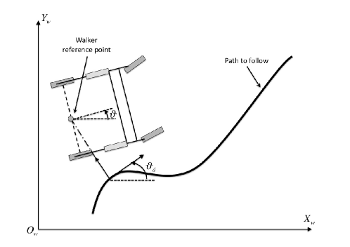
Figure 1: Vehicle to path configuration and reference frames.

Let ${\bf x}=[x,\,y,\,\theta]^{T}\in\mathbb{R}^{2}\times S$ be the kinematic configuration of the cart, where $(x,\,y)$ are the coordinates of the mid–point of the rear wheels axle in $\Pi$ and $\theta$ is the orientation of the vehicle w.r.t. the $X_{w}$ axis (see Fig. 1). The dynamic model of the FriWalk can be assimilated to a unicycle

$$\begin{bmatrix}\dot{x}\\ \dot{y}\\ \dot{\theta}\\ \dot{v}\\ \dot{\omega}\end{bmatrix}=\begin{bmatrix}v\cos(\theta)\\ v\sin(\theta)\\ \omega\\ \frac{F}{m}\\ \frac{N}{J}\end{bmatrix}\Leftrightarrow\begin{bmatrix}\dot{s}\\ \dot{l}\\ \dot{\tilde{\theta}}\\ \dot{v}\\ \dot{\tilde{\omega}}\end{bmatrix}=\begin{bmatrix}\gamma\\ v\sin(\tilde{\theta})\\ \omega-c(s)\gamma\\ \frac{F}{m}\\ \frac{N}{J}-c(s)\ddot{s}-c(s)^{\prime}\gamma\end{bmatrix}$$ (1)

where $v$ is the forward velocity of the vehicle and $\omega$ its angular velocity. $F$ is the external force acting on the vehicle along the direction of motion, $N$ is the external torque about the $Z_{w}$-axis, $m$ and $J$ are the mass and moment of inertia of the cart. Moreover, $s$ is the curvilinear abscissa along the path, $l$ is the distance between the origin of the Frenet frame and the reference point of the FriWalk along the $Y$-axis of the Frenet frame, and $\theta_{d}$ is the angle between the $X_{w}$-axis and the $X$-axis of the Frenet frame (see Fig. 1). Therefore, $\tilde{\theta}=\theta-\theta_{d}$ and $\tilde{\omega}=\dot{\tilde{\theta}}$. Furthermore, the path curvature is defined as $c(s)={d\theta_{d}(s)}/{ds}$, while $c^{\prime}(s)=dc(s)/ds$. Finally,

$$\gamma=\frac{v\cos(\tilde{\theta})}{1-c(s)l}.$$

It is worthwhile to note that this model is commonplace in the literature [10, 23, 13].

By denoting with $\tau_{r}$ and $\tau_{l}$ the torques applied on the right and left rear wheels, respectively, we have the invertible linear relations

$$F=\frac{\tau_{r}+\tau_{l}}{r}\,\,\,\mbox{and}\,\,\,N=\frac{(\tau_{r}-\tau_{l})d}{2r}.$$ (2)

where $d$ is the axle length. In particular, denoting with $M_{(\cdot)}$ the quantity $M$ of the left or right side of the trolley and assuming that $\alpha_{(\cdot)}$ is the rotation angle of the rear wheels, the wheel dynamics can be described by $J_{w}\ddot{\alpha}_{(\cdot)}=\tau_{(\cdot)}$, where $J_{w}$ is the equivalent moment of inertia of the wheel.

3.2 Braking System

The available input variables are the independent braking torques $\tau_{l}^{b}$ and $\tau_{r}^{b}$, acting on the left and right wheels, respectively. Similarly to [7, 17], the braking torques ranges between zero, i.e., the wheel rotates freely, to a maximum value. More precisely, let the torques acting on (2) be expressed by

$$\tau_{(\cdot)}=\tau_{(\cdot)}^{h}+\tau_{(\cdot)}^{b}-b_{w}\dot{\alpha}_{(\cdot)},$$ (3)

which is the sum of the torque $\tau_{(\cdot)}^{h}$, that results from the force exerted by the user on the handles and transmitted to the wheel hub through the mechanical structure of the walker, of the term $-b_{w}\dot{\alpha}_{(\cdot)}$, accounting for the rolling resistance that opposes to the wheel rotation (thus having $b_{w}$ as the viscous friction coefficient around the wheel rotation axle) and of braking action $\tau_{(\cdot)}^{b}$. Notice that pure rolling assumption is supposed to hold. Similarly to [7], the braking action is modeled as a dissipative system, i.e.,

$$\tau_{(\cdot)}^{b}=-b^{b}_{(\cdot)}\dot{\alpha}_{(\cdot)},$$ (4)

where $b^{b}_{(\cdot)}\in[0,\,b_{\max}]$ are controllable variables determining the viscous frictions of the brakes. Whenever $\dot{\alpha}_{(\cdot)}=0$, to model the fact that the brake has sufficient authority to keep the wheel at rest, we assume that

$$\tau_{(\cdot)}^{b}=-c^{b}_{(\cdot)}\tau^{h}_{(\cdot)},$$ (5)

where $c^{b}_{(\cdot)}\in[0,1]$ is an additional controllable variable acting when $\dot{\alpha}_{(\cdot)}=0$. In case of servo brakes, coefficients $b^{b}_{(\cdot)}$ and $c^{b}_{(\cdot)}$ can be changed by varying the input current, thus allowing the control system to suitably modulate the braking torque [7].

By direct experimental measurements made on the system at hand, we have observed that the torques applied by the user to the mechanical system are negligible with respect to the maximum braking action. Moreover, the inertia of the system as well as the maximum forward velocity $v$ are limited. As a consequence, the time needed to stop the wheel rotation is negligible and, hence, it can be assumed $\omega_{(\cdot)}=0$ whenever the braking system is fully active.

Due to the described platform, the control law we are designing deals with a limited set of control inputs. More precisely, the admitted control values for each wheel are either $c_{(\cdot)}^{b}=0$ and $b^{b}_{(\cdot)}=0$ or $c_{(\cdot)}^{b}=1$ and $b_{(\cdot)}^{b}=b_{\max}$, i.e., no brake or full brake. If by chance the brake is fully active on the right wheel, from (3) it follows that $\omega_{r}(t)\rightarrow 0$. Hence, the vehicle will end-up in following a circular path with fixed curvature radius $R=d/2$, where $d$ is the rear wheel inter-axle length, travelled in clockwise direction if $v>0$ (counter-clockwise for $v<0$). The circular path with the same radius $R$ will be instead followed in counter-clockwise direction if the left brake is fully active and $v>0$ (clockwise for $v<0$). As a consequence, in all the cases of active braking system, $\omega=v/R$. If no braking action is applied at all, the user will drive the FriWalk uncontrolled. On the other hand, if both brakes are fully active, the vehicle will reach the full stop. From a control perspective, the previous model turns into a nonholonomic nonlinear vehicle with limited curvature and quantised inputs: turn left, turn right, move freely or stop.

3.3 Problem Formulation

We require the walker to converge to our planned path defined in $\Pi$, which we will assume to be smooth (i.e., with a well defined tangent on each point) and with a known curvature. The planned path is typically composed of straight segments and circular arcs connected with clothoids. The problem to solve is formalised as a classic asymptotic stability problem:

$$\lim_{t\rightarrow+\infty}l(t)=0,\,\,\,\mbox{and}\,\,\,\lim_{t\rightarrow+\infty}\tilde{\theta}(t)=0.$$ (6)

In general, the dynamic path following problem requires the design of a stabilising control law $F(t)$ and $N(t)$ for the system in (1). Due to (2), (3), (4) and (5), such a solution requires a proper control low for the control inputs $c_{r}^{b}$, $b^{b}_{r}$, $c_{l}^{b}$ and $b^{b}_{l}$.

4 Approaching the Path

The first part of the solution proposed in this paper relies on the hybrid automaton designed in [14], which proposes a minimum length trajectory to reach a desired path for limited curvature unicycle-like vehicles. We first summarise the key points of this algorithm (for the reader convenience) and then we move to the description of its generalisation for the problem at hand.

4.1 Hybrid Solution

The solution proposed by Ballucchi et al. [14] is based on a hybrid feedback controller solving (6) for unicycle-like vehicles with bounded curvature radius. In particular, the solution there proposed faces the problem of driving a Dubin’s car to a generic path assuming a maximum known curvature for the path. The authors show that their hybrid controller is stable with respect to the path-related coordinates $(\tilde{l},\tilde{\theta})$, where $\tilde{l}=l/R$ and $R$ is the fixed maximum turning radius of the vehicle. The controller automaton comprises three different manoeuvres, i.e., Go Straight, Turn Right and Turn Left, which are defined in terms of the angular velocity $\tilde{\omega}$ of (1) as

$$\left\{\begin{array}[]{ll}\tilde{\omega}=0&\mbox{if {\em Go Straight}}\\ \tilde{\omega}=-\frac{v}{R}&\mbox{if {\em Turn Right}}\\ \tilde{\omega}=\frac{v}{R}&\mbox{if {\em Turn Left}}\end{array}\right.$$

assuming the forward input $v>0$ is known. The solution can then be straightforwardly mapped onto the control variables available for our specific problem, i.e.,

$$\left\{\begin{array}[]{ll}b_{r}^{b}=b_{l}^{b}=c_{r}^{b}=c_{l}^{b}=0&\mbox{if {\em Go Straight},}\\ b_{r}^{b}=b_{\max}\wedge c_{r}^{b}=1\wedge b_{l}^{b}=c_{l}^{b}=0&\mbox{if {\em Turn Right},}\\ b_{l}^{b}=b_{\max}\wedge c_{l}^{b}=1\wedge b_{r}^{b}=c_{r}^{b}=0&\mbox{if {\em Turn Left},}\\ b_{r}^{b}=b_{l}^{b}=b_{\max}\wedge c_{r}^{b}=c_{l}^{b}=1&\mbox{if {\em Stop}.}\end{array}\right.$$ (7)

The hybrid automaton comprises three states, in which the three manoeuvres are coded according to the initial configuration of the vehicle. To this end, the state space $(\tilde{l},\tilde{\theta})$ is suitably partitioned into a set of non-overlapping regions. In each region only one of the three manoeuvres is active. For the sake of completeness we report a typical qualitative trajectory of the robot in the phase portrait $(\tilde{l},\tilde{\theta})$ in Figure 2, trajectory $E$ (solid thick line).

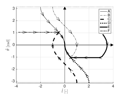
Figure 2: Phase portrait for a set of manoeuvres of the generalised hybrid controller [14] for $\delta=\pi/3$.

The first part of the manoeuvre is obtained by the Turning State, in which the robot performs a Turn Right with minimum radius curvature until it is oriented towards the path to reach (a linear segment in this example), with $\tilde{\theta}=\delta$. Then the robot proceeds towards the path in the Straight state performing a Go Straight manoeuvre and, finally, if switches to the Controlled state, in which it rotates performing a final Turn Left manoeuvre and, hence, solving the problem. Once the robot reaches the path with the correct orientation, it permanently remains there providing that the path curvature is feasible according to the minimum curvature radius constraint.

4.2 Generalised Hybrid Solution

In [14] the choice of the angle of approach $\delta=\pi/2$ is dictated by the necessity to reach the desired path with the minimum travelled distance. Our first generalisation, which is useful for our specific application since it adds an additional degge of freedom during the approaching path manoeuvre, is to consider the angle of approach $\delta$ as a design parameter. In order to extend the results of [14] to this broader set of possibilities, let us first depict in the phase portrait the trajectories followed by the robot when it continuously rotates on circles with minimum radius $R$ (Figure 3), i.e., the trajectories described in the Turning State.

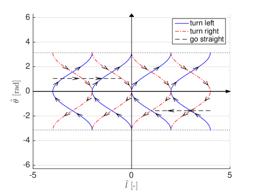
Figure 3: Phase portrait for the Turning State (solid lines). The graph is reported for $\tilde{l}=\{-4,-2,0,2,4\}$. The dashed line corresponds to the Straight state for a generic choice of $\delta$.

Notice that circles with any $\bar{R}>R$, similar graphs are derived. Furthermore, notice that the angles $\tilde{\theta}\in[-\pi,\pi)$. The dashed lines in Figure 3 represent a possible choice of $\delta\in(-\pi,\pi)$. It is now evident that the sequence of states to reach the path will be given again by: Turning State - Straight state - Controlled state. Each of them can be of zero length. More precisely, by generalising the boundary functions reported in [14] to the case of a generic $\delta$ as:

$$\begin{split}\sigma_{R}(\tilde{l},\tilde{\theta})&=\tilde{l}+1-\cos(\tilde{\theta}),\\ \sigma_{L}(\tilde{l},\tilde{\theta})&=\tilde{l}-1+\cos(\tilde{\theta}),\\ \sigma_{N}(\tilde{l},\tilde{\theta},\delta)&=\tilde{l}+1-2\cos(\delta)+\cos(\tilde{\theta}),\\ \sigma_{P}(\tilde{l},\tilde{\theta},\delta)&=\tilde{l}-1+2\cos(\delta)-\cos(\tilde{\theta}),\end{split}$$ (8)

the manoeuvre switching curves are defined, and depicted in Figure 4.

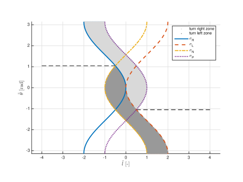
Figure 4: Boundary functions and state space partition induced by the boundary function for $\delta=\pi/3$.

Those boundaries define the partition of the state space, reported in the same Figure 4 with dark and light grey colours. In light of this partition, obtained for $\delta=\pi/3$, from the light grey region the sequence will be Turning State (on the right or clockwise) - Controlled state (turning on the left or counterclockwise), whose trajectory is named $B$ in Figure 2 (dash-dotted line). The same happens, but with opposite rotations, from the dark grey region ($C$ trajectory in Figure 2, dashed thick line). On the left boundary of the light grey region ($\sigma_{R}(\tilde{l},\tilde{\theta})$ of (8)), the manoeuvre comprises only the Controlled state (turning on the right, trajectory $A$ in Figure 2, solid line), while from the right boundary of the dark grey region ($\sigma_{L}(\tilde{l},\tilde{\theta})$ of (8)), the manoeuvre comprises again only the Controlled state (turning on the left, trajectory $D$ in Figure 2, dotted thick line). From the dashed line of Figure 4, the sequence is Straight state - Controlled state (trajectory $F$ in Figure 2, dash-dotted thick line), while from all the other position the sequence of states is complete (trajectory $E$ in Figure 2, solid thick line). It is worthwhile to note that the regions reverted for $v<0$. To conclude, we have shown that the generalisation of the approaching angle to a generic $\delta\in(-\pi,\pi)$ still preserves the stability property of [14]. Nonetheless, it offers a great possibilities for the design of the control law in the spirit recalled in the Introduction.

5 Following the Path

After the approaching phase is completed, the vehicle reaches the proximity of the path with a minimal set of manoeuvres and with a generic $\delta$. The solution provided by [14] to finally stabilise the robotic platform on the path, even for a generic angle $\delta$, has two major problems: a) it is perceived as unnatural by the user; b) if an error on the switching point exists, the vehicle generates a set of repeated uncomfortable curves, similar to the solid line reported in Figure 6. In order to overcome this limitation and provide a smooth asymptotic convergence to the path, we present a further extension of the hybrid automata by considering state dependent $\delta$ functions. Having a state dependent approaching angle to lead the evolution of $\tilde{\theta}(t)$ is a common solution for nonholonomic path following control problems. Just to mention a few notable solutions, [13] proposes a Lyapunov-based control law design to govern the torque $N$ in (1) and lead the vehicle to track the reference angle $\delta(\tilde{l},v)$ defined as an odd smooth function of $\tilde{l}$. A similar solution based on a nonlinear system expressed in chained-form has been also presented in [11] for a vehicle with saturated actuation. The hybrid feedback controller here proposed extends the previous results on unicycle-like vehicles to quantised control inputs with customisable approaching angle. More importantly, it will be shown that the control law of [13] can be emulated without any estimate of the user applied forces and torques and without a precise modulation of the braking force (contrary to the solution reported in [8])), as reported in Theorem 1. In what follows and without loss of generality, we focus on $v(t)>0$, $\forall t$ (therefore, $\delta(\tilde{l},v)$ simplifies to $\delta(\tilde{l})$).

Theorem 1

For any function $\delta(\tilde{l})$ continuous, limited $\delta(\tilde{l})\in(-\pi,\pi)$, with $-\mbox{sign}(\tilde{l})\frac{\partial\delta(\tilde{l})}{\partial\tilde{l}}\geq 0$ and $\tilde{l}\delta(\tilde{l})>0$, $\forall\tilde{l}\neq 0$, the origin of the space $(\tilde{l},\tilde{\theta})$ is asymptotically stable.

Proof Let us suppose that the robot is not able to reach the region $\tilde{\theta}=\delta(\tilde{l})$. In light of the previous analysis and, in particular, by means of the boundary functions (8) and the region partition of Figure 4, the vehicle is on either $\sigma_{L}(\tilde{l},\tilde{\theta})$ or $\sigma_{R}(\tilde{l},\tilde{\theta})$. Therefore, the hybrid system is in the Controlled state and the robot reaches $\tilde{\theta}=\delta(\tilde{l})$ only in the origin.

Hence, let us suppose that for a certain finite time instant $\tilde{\theta}=\delta(\tilde{l})$. If $|\dot{\delta}(\tilde{l})|\leq v/R$, $\forall\tilde{l}$, i.e., the commanded $\delta(\tilde{l})$ has instantaneous curvatures that are less than $R$, the vehicle remains on the region $\tilde{\theta}=\delta(\tilde{l})$ by switching continuously between the Turning State and the Go Straight. Notice that the hybrid state Controlled state is never reached, in this case.

However, it may happen that $|\dot{\delta}(\tilde{l})|>v/R$ for certain values $\tilde{l}>\widehat{\tilde{l}}$. In such a case, the reference of $\delta(\tilde{l})$ is unfeasible for the limited turning radius vehicle. Let us define with $\bar{t}$ the time in which the vehicle departs from the unfeasible region $\tilde{\theta}=\delta(\tilde{l})$ due to the limited turning radius $R$. Since $\delta(\tilde{l})$ is a smooth odd function of $\tilde{l}$ and since the turning manoeuvre is symmetric with respect to the $\tilde{\theta}=0$ axis (see Figure 3), when the vehicle re-enters into the region $\tilde{\theta}=\delta(\tilde{l})$ after a turning at time $\widehat{t}>\bar{t}$, both $|\tilde{l}(\widehat{t})|<|\tilde{l}(\bar{t})|$ and $|\tilde{\theta}(\widehat{t})|<|\tilde{\theta}(\bar{t})|$ hold. As a consequence, there exist a time $t$ such that $\tilde{l}(t)<\widehat{\tilde{l}}$, hence $|\dot{\delta}(\tilde{l})|\leq v/R$ and, finally, the previous situation holds.

We are now able to prove the stability of the proposed feedback control law using the Lyapunov stability theory. To this end, let us define the following Lyapunov function candidate

$$V(\tilde{l},\tilde{\theta})=\frac{1}{2}\left(\tilde{l}^{2}+\tilde{\theta}^{2}\right),$$ (9)

which is positive definite with respect to the subspace of interest. Using (1) it is immediate to note that $\dot{V}(\tilde{l},\tilde{\theta})$ is negative definite in the Controlled state and whenever $\tilde{\theta}=\delta(\tilde{l})$, which proves the convergence towards the origin from any initial condition.

Figure 5 depicts the phase portrait from various initial configurations for $\delta(\tilde{l})=\frac{\pi}{2}\tanh(\tilde{l})$, i.e., an always feasible approaching angle.

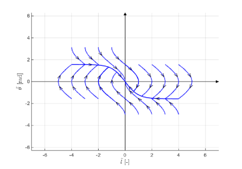
Figure 5: Phase portrait from various initial configurations when $\delta(\tilde{l})=\frac{\pi}{2}\tanh(\tilde{l})$ is feasible reference angle.

Instead, an example of an unfeasible $\delta(\tilde{l})$ is reported in Figure 6, for both the phase portrait and the Cartesian trajectory followed by the vehicle.

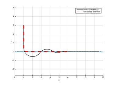
(a)

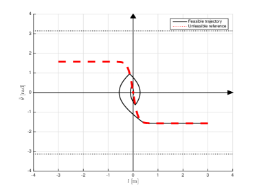
(b)

Figure 6: Vehicle trajectory (a) and phase portrait (b) (black lines) for an unfeasible reference angle $\delta(\tilde{l})$ (green lines).

6 Simulations Results

To show the effectiveness of the proposed solution, simulations are reported for a generic path. Figure 7 reports the trajectory followed by the vehicle starting with an initial configuration $(x,y,\theta)=(1,5,0)$.

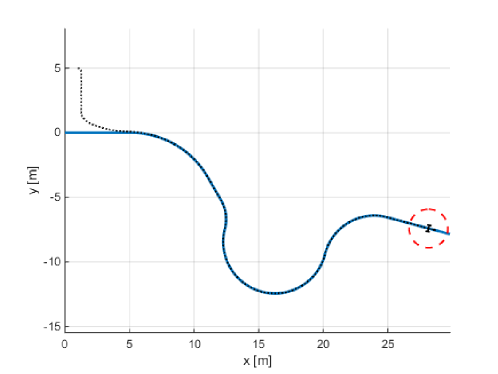
Figure 7: Example of a controlled trajectory.

The final position of the robot on the path is highlighted with a dashed circle. The function $\delta(\tilde{l})=\frac{\pi}{2}\tanh(\tilde{l})$ is adopted. The distance to the path $l$ and relative angle $\tilde{\theta}$ are reported in Figure 8.

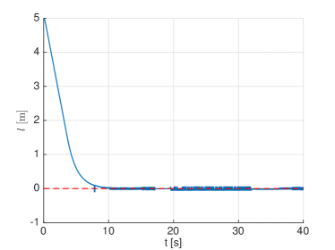
(a)

(b)

Figure 8: Time evolution of the variables $l$ (a) and $\tilde{\theta}$ (b) for the trajectory depicted in Figure 7.

The high frequency oscillations are due to the continuous switching between the Turning State and the Go Straight hybrid states, which is necessary to approximate a generic curvature path.

7 Conclusions

In this paper we have presented a passive control strategy for a robotic walking assistant that guides a senior user with mobility problems along a planned path. The control strategy exploits the electromechanical brakes mounted on the back wheels of the walker. Due to cost limits, the solutions proposed is based on a simple actuation strategy in which the braking system is controlled with a bang-bang control. We show that it is possible to secure a gentle and smooth path following and to control the vehicle in feedback towards the desired path by applying two different strategies: when the platform is far away from the path, we execute an approach phase in which the walker converges toward the platform with a specified angle; when it comes in proximity of the platform, the control strategy switches to a path tracking mode, which uses the four control actions to converge toward the path with an angle which is a function of the state. We have further shown that it is possible to mimic a dynamic feedback control law without collecting dynamic measures on the system, hence lowering down its costs.

Future developments will mainly focus on the application of the proposed algorithm on the actual system and on the reduction of the annoying switchings among the different states of the hybrid automata for generic curves. Another point that serves some further investigations is related to the user behaviour when it is commanded to go straight. In such a case, the strateg should be modified to account for unreliable and uncooperative users.

References

- [1] “ACANTO: A CyberphysicAl social NeTwOrk using robot friends,” http://www.ict-acanto.eu/acanto, February 2015, EU Project.
- [2] A. Balluchi, A. Bicchi, A. Balestrino, and G. Casalino, “Path tracking control for dubin’s cars,” in Proc. IEEE Conf. on Robotics and Automation (ICRA), vol. 4, Apr 1996, pp. 3123–3128.
- [3] J.-P. Laumond, Robot motion planning and control. Lectures Notes in Control and Information Sciences 229, 1998, vol. 3.
- [4] C. Samson, “Control of chained systems application to path following and time-varying point-stabilization of mobile robots,” IEEE Trans. on Automatic Control, vol. 40, no. 1, pp. 64–77, 1995.
- [5] M. Aicardi, G. Casalino, A. Bicchi, and A. Balestrino, “Closed loop steering of unicycle like vehicles via lyapunov techniques,” IEEE Robotics & Automation Magazine, vol. 2, no. 1, pp. 27–35, 1995.
- [6] O. Sordalen and C. De Wit, “Exponential control law for a mobile robot: extension to path following,” in Proc. IEEE Conf. on Robotics and Automation (ICRA), vol. 3, May 1992, pp. 2158–2163.
- [7] Y. Hirata, A. Hara, and K. Kosuge, “Motion control of passive intelligent walker using servo brakes,” IEEE Transactions on Robotics, vol. 23, no. 5, pp. 981–990, 2007.
- [8] D. Fontanelli, A. Giannitrapani, L. Palopoli, and D. Prattichizzo, “Unicycle Steering by Brakes: a Passive Guidance Support for an Assistive Cart,” in Proc. IEEE Int. Conf. on Decision and Control. Florence, Italy: IEEE, 10-13 Dec. 2013, pp. 2275–2280.
- [9] M. Martins, C. Santos, A. Frizera, and R. Ceres, “A review of the functionalities of smart walkers,” Medical engineering & physics, vol. 37, no. 10, pp. 917–928, 2015.
- [10] A. De Luca, G. Oriolo, and C. Samson, “Feedback control of a nonholonomic car-like robot,” in Robot motion planning and control. Springer, 1998, pp. 171–253.
- [11] Z.-P. Jiang, E. Lefeber, and H. Nijmeijer, “Saturated stabilization and tracking of a nonholonomic mobile robot,” Systems & Control Letters, vol. 42, no. 5, pp. 327–332, 2001.
- [12] A. Lapierre and D. Soetano, “Nonlinear path-following control of an AUV,” Ocean engineering, vol. 34, no. 11, pp. 1734–1744, 2007.
- [13] D. Soetanto, L. Lapierre, and A. Pascoal, “Adaptive, non-singular path-following control of dynamic wheeled robots,” in IEEE Conf. on Decision and Control, vol. 2. IEEE, 2003, pp. 1765–1770.
- [14] A. Balluchi, A. Bicchi, and P. Soueres, “Path-following with a bounded-curvature vehicle: a hybrid control approach,” International Journal of Control, vol. 78, no. 15, pp. 1228–1247, 2005.
- [15] P. Soueres, A. Balluchi, and A. Bicchi, “Optimal feedback control for route tracking with a bounded-curvature vehicle,” International Journal of Control, vol. 74, no. 10, pp. 1009–1019, 2001.
- [16] T. Pilutti, G. Ulsoy, and D. Hrovat, “Vehicle steering intervention through differential braking,” in Proceedings of the 1995 American Control Conference, vol. 3, 1995, pp. 1667–1671.
- [17] M. Saida, Y. Hirata, and K. Kosuge, “Development of passive type double wheel caster unit based on analysis of feasible braking force and moment set,” in Proceedings of the 2011 IEEE/RSJ International Conference on Intelligent Robots and Systems, 2011, pp. 311–317.
- [18] U. Cortes, C. Barrue, A. B. Martinez, C. Urdiales, F. Campana, R. Annicchiarico, and C. Caltagirone, “Assistive technologies for the new generation of senior citizens: the share-it approach,” International Journal of Computers in Healthcare, vol. 1, no. 1, pp. 35–65, 2010.
- [19] P. Nazemzadeh, D. Fontanelli, D. Macii, T. Rizano, and L. Palopoli, “Design and Performance Analysis of an Indoor Position Tracking Technique for Smart Rollators,” in Indoor Positioning and Indoor Navigation (IPIN). Montbeliard, France: IEEE GRSS, 28-31 Oct. 2013, to appear.
- [20] P. Nazemzadeh, F. Moro, D. Fontanelli, D. Macii, and L. Palopoli, “Indoor Positioning of a Robotic Walking Assistant for Large Public Environments,” IEEE Trans. on Instrumentation and Measurement, vol. 64, no. 11, pp. 2965–2976, Nov 2015.
- [21] A. Colombo, D. Fontanelli, A. Legay, L. Palopoli, and S. Sedwards, “Motion planning in crowds using statistical model checking to enhance the social force model,” in Decision and Control (CDC), 2013 IEEE 52nd Annual Conference on. IEEE, 2013, pp. 3602–3608.
- [22] ——, “Efficient customisable dynamic motion planning for assistive robots in complex human environments,” Journal of Ambient Intelligence and Smart Environments, vol. 7, no. 5, pp. 617–633, 2015.
- [23] L. Lapierre and D. Soetanto, “Nonlinear path-following control of an AUV,” Ocean engineering, vol. 34, no. 11, pp. 1734–1744, 2007.