X-ray-binary spectra in the lamp post model

Abstract

Context. The high-energy radiation from black-hole binaries may be due to the reprocessing of a lamp located on the black hole rotation axis and emitting X-rays. The observed spectrum is made of three major components: the direct spectrum traveling from the lamp directly to the observer; the thermal bump at the equilibrium temperature of the accretion disk heated by the lamp; and the reflected spectrum essentially made of the Compton hump and the iron-line complex.

Aims. We aim at computing accurately the complete reprocessed spectrum (thermal bump + reflected) of black-hole binaries over the entire X-ray band. We also determine the strength of the direct component. Our choice of parameters is adapted to a source showing an important thermal component. We are particularly interested in investigating the possibility to use the iron-line complex as a probe to constrain the black hole spin.

Methods. We compute in full general relativity the illumination of a thin accretion disk by a fixed X-ray lamp along the rotation axis. We use the ATM21 radiative transfer code to compute the local, energy-dependent spectrum emitted along the disk as a function of radius, emission angle and black hole spin. We then ray trace this local spectrum to determine the final reprocessed spectrum as received by a distant observer. We consider two extreme values of the black hole spin ($a=0$ and $a=0.98$) and discuss the dependence of the local and ray-traced spectra on the emission angle and black hole spin.

Results. We show the importance of the angle dependence of the total disk specific intensity spectrum emitted by the illuminated atmosphere when the thermal disk emission if fully taken into account. The disk flux, together with the X-ray flux from the lamp, determines the temperature and ionization structure of the atmosphere. High black hole spin implies high temperature in the inner disk regions, therefore the emitted thermal disk spectrum fully covers the iron-line complex. As a result, instead of fluorescent iron emission line, we locally observe absorption lines produced in the hot disk atmosphere. Absorption lines are narrow and disappear after ray tracing the local spectrum.

Conclusions. Our results mainly highlight the importance of considering the angle dependence of the local spectrum when computing reprocessed spectra, as was already found in a recent study. The main new result of our work is to show the importance of computing the thermal bump of the spectrum, as this feature can change considerably the observed iron-line complex. Thus, in particular for fitting black hole spins, the full spectrum, and not only the reflected part, should be computed self-consistently.

1 Introduction

It is probable that X-ray spectra emitted by black-hole binaries and active galactic nuclei contain relativistic signatures due to the proximity of the emission region to the central black hole. In particular, the distortion of the Fe K line has been since a long time advocated to be due to relativistic effects (Fabian et al. 1989; Reynolds & Nowak 2003). This feature of the spectrum is used to constrain the spin parameter of black holes (Reynolds 2014).

The observed X-ray spectra show two components, a soft and a hard one, that can be naturally explained in the scenario where an accretion disk is accompanied by some Comptonizing region, which can be typically either a hot corona sandwiching the inner region of the disk (Haardt & Maraschi 1991), a hot inner flow occupying the regions close to the black hole with the disk being truncated to some radius (Zdziarski & Gierliński 2004; Done et al. 2007), or the base of a jet located on the rotation axis of the black hole (see among many others Matt et al. 1991; Martocchia & Matt 1996; Markoff et al. 2005). In this article we will only consider this third option, the so-called lamp post model.

Our aims are (1) to compute the flux of illuminating radiation from this lamp to the accretion disk, (2) to compute the reflected intensity spectrum due to the reprocessing of the illuminating flux by the disk and (3) to ray trace this to a distant observer. Many works have been investigating these various points in the past. Point (1) and (3) essentially deal with the effect of light bending from a lamp post to the illuminated accretion disk and then to the distant observer (see among others Reynolds et al. 1999; Ruszkowski 2000; Miniutti et al. 2003; Miniutti & Fabian 2004; Fukumura & Kazanas 2007; Wilkins & Fabian 2012; Dauser et al. 2013; Dovciak et al. 2014). Point (2) requires solving the complex radiative transfer in the illuminated accretion disk and has also been investigated by many authors since quite a long time, taking into account either Newtonian or general-relativistic illumination, solving the radiative transfer equations in a Newtonian framework, and assuming the reflection from a constant-density slab (see among others George & Fabian 1991; Matt et al. 1991; Ross & Fabian 1993; Zycki & Czerny 1994; Czerny & Zycki 1994; Magdziarz & Zdziarski 1995; Poutanen et al. 1996; Niedźwiecki & Życki 2008; García & Kallman 2010). In addition, the assumption of a stratified gas being in hydrostatic equilibrium is more realistic but more complex from a numerical point of view (Nayakshin & Kallman 2001; Ballantyne et al. 2001; Różańska et al. 2002; Różańska & Madej 2008; Różańska et al. 2011). In particular, Różańska & Madej (2008, together with the subsequent works of the same authors) solve the radiative equilibrium which was not dealt with previously, to our knowledge, by any other group. The most advanced attempt to take into account points (1), (2) and (3) is the work of García et al. (2014), which was the main motivation for the development of this article. These authors, however, still consider the reflection from a constant-density slab and that the illumination is incident on the disk at a constant angle equal to $45^{\circ}$.

This article’s treatment of point (1) and (3) is close to the treatment of Dauser et al. (2013) and García et al. (2014). However, there are two important differences. The first one is that we take into account the redshift effect on the frequency cut-offs assumed in the lamp frame (see the discussion in Niedźwiecki et al. 2016). The second one is that we do not assume a $45^{\circ}$ incidence of the illumination but rather consider the true direction of incidence to compute the mean illuminating intensity. As far as point (2) is concerned, there is an important difference between our treatment and the one of García et al. (2014), which is the main reason for us to revisit this topic. We are computing local intensity spectra using the code ATM21 of Różańska et al. (2011). This code solves the hydrostatic and radiative equilibria of the disk self-consistently, taking into account a slim disk solution (Sa̧dowski et al. 2011) with a given spin parameter. The full spectrum, including the thermal bump due to the radiation of the accretion disk heated by the lamp, is computed. García et al. (2014) do not solve the hydrostatic equilibrium and rather assume a constant-density slab. Moreover, they only compute the reflected part of the spectrum and do not consider the thermal bump. As far as the value of spin is concerned, this means that only the inner radius of the disk (supposed to be at the innermost stable circular orbit, the ISCO, which depends on the spin parameter) takes spin into account in García et al. (2014). Besides this, the disk physics is the same whatever the spin. This is an important simplification and it was highlighted by Nayakshin & Kallman (2001) that the two options (considering a constant-density slab or solving the hydrostatics of the disk) do not lead to the same predictions. Moreover, as we are particularly interested in taking as much as possible general-relativistic effects into account (particularly spin effects), we believe that it is important to solve the hydrostatic equilibrium for the particular value of spin parameter assumed for the central black hole. We note that our treatment is not 100% relativistic as the radiative transfer is solved in a Newtonian spacetime (similarly as in García et al. 2014). However, given that point (2) is restricted to local phenomena, we do not think that this may have important consequences on the modeled spectra. We thus believe that the simulations we present are among the most realistic to date, as far as taking spin effect into account is concerned. Understanding spin effects imprinted in the reflected spectrum is particularly important given that the Fe K line is one of the probe of black hole spins and will be used by high-precision future mission like Hitomi (formerly ASTRO-H, Takahashi et al. 2014; Miller et al. 2014; Reynolds et al. 2014) and ATHENA (Nandra et al. 2013; Dovciak et al. 2013).

This article aims at simulating accurately the observed spectrum generated by a simple lamp post scenario. Our first goal is to compute accurately the flux emanating from the lamp and illuminating the disk (Section 2). We will compute the illuminating flux either in a Newtonian spacetime or in the Kerr spacetime with spin parameter $a=0$ and $a=0.98$. This allows us to compare the resulting local specific intensity reflected spectrum, emitted by the disk at some emission angle towards the Earth, for these three kinds of illuminations. Our second goal is to compute the local reflected spectrum due to the reprocessing of the illuminating flux by the disk (Section 3.1). Our third goal is to ray trace this local spectrum to a distant observer (Section 3.2). Finally, Section 4 gives conclusions and perspectives.

2 Illuminating mean intensity

We consider a spherical source of radiation (the lamp) located along the rotation axis of a black hole, at some coordinate $z$. The radius of the spherical source is assumed small enough so that it is perceived as point-like by any observer rotating with the disk. In our simulations, this radius is $R=0.25\,M$, where $M$ is the black hole mass. We consider a set of corotating observers in the disk at several coordinate radii $r$. The global accretion disk model considered for computing the reflected spectrum is a slim disk as described by Sa̧dowski et al. (2011) with an accretion rate $\dot{m}=0.01\,\dot{m}_{\mathrm{Edd}}$, where the Eddington accretion rate defined as $\dot{m}_{\mathrm{Edd}}=16\,L_{\mathrm{Edd}}/c^{2}$. For this moderate accretion rate, the disk is very thin ($H/r\approx 0.05$) and the gas follows nearly Keplerian orbits. We thus consider a set of Keplerian observers, corotating with the disk at the local Keplerian angular velocity. For each of these observers we perform backwards-in-time ray tracing from the observer towards the lamp in order to determine the illuminating flux received by each observer.

For all ray-tracing computations presented in this article, we use the open-source GYOTO code (Vincent et al. 2011). Photons are traced by integrating the geodesic equation using a Runge-Kutta-Fehlberg adaptive-step integrator at order 7/8 (meaning that the method is 8th order, with an error estimation at 7th order).

We consider a lamp emitting isotropically in its rest frame. This is obviously a simplifying hypothesis that is most likely not to be satisfied in a realistic context. Indeed, the X-ray radiation from the lamp is likely to be produced by the Comptonization of photons emitted by the accretion disk (see e.g. the recent discussion in Dovciak & Done 2015). This process would lead to anisotropic radiation. Moreover, we also neglect the motion of the source and it has already been discussed in the literature that the lamp motion affects the reflected spectrum (Wilkins & Fabian 2012; Dauser et al. 2013). A realistic treatment of the Comptonization of the disk’s photons by a moving source goes beyond the scope of the present paper. The lamp is thus emitting radiation isotropically in its rest frame following a power-law spectrum over the X-ray band

$$I_{\nu}^{\mathrm{lamp}}=A\nu_{\mathrm{lamp}}^{-\alpha},\quad\nu_{\mathrm{lamp}}\in[\nu_{\mathrm{lamp,1}},\nu_{\mathrm{lamp,2}}]$$ (1)

where $\nu_{\mathrm{lamp}}$ is the emitted frequency as measured in the rest frame of the lamp, $\alpha$ is the spectral index and $A$ is a normalizing constant to be determined later on. The frequencies $\nu_{\mathrm{lamp,1}}$ and $\nu_{\mathrm{lamp,2}}$ are the limits of the illumination band. Once the ray-tracing computation has been performed, it is possible to determine what is the angle $i$ in each Keplerian observer’s rest frame between the local normal and the direction of the lamp on sky, as well as the value of the specific intensity received by each Keplerian observer corotating at coordinate radius $r$

$$I_{\nu}^{\mathrm{disk}}(i,r)=Ag^{3+\alpha}\nu_{\mathrm{disk}}^{-\alpha},\quad\nu_{\mathrm{disk}}\in[\nu_{\mathrm{disk,1}},\nu_{\mathrm{disk,2}}]$$ (2)

where $\nu_{\mathrm{disk}}$ is the observed frequency, as measured in the rest frame of the Keplerian observer and $g=\nu_{\mathrm{disk}}/\nu_{\mathrm{lamp}}$ is the redshift factor. In particular, the limiting frequencies in the disk frame are obtained from their lamp-frame counterparts by using $\nu_{\mathrm{disk,i}}=g\,\nu_{\mathrm{lamp,i}}$. Figure 1 illustrates the geometry and the image of the lamp as seen by the given Keplerian observer.

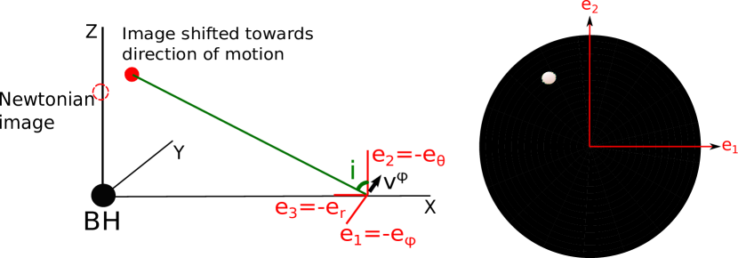
Figure 1: Left: geometry of the lamp post model. The velocity $v^{\varphi}$ is the Keplerian velocity of the corotating observer. The triad ($\boldsymbol{e_{1}}$,$\boldsymbol{e_{2}}$,$\boldsymbol{e_{3}}$) is the local rest frame of the observer. The angle $i$ lies between the direction of the local normal and the direction of the lamp as seen by the observer. Right: image (map of the quantity $g^{3+\alpha}$ as defined in Eq. 2) of the lamp as observed by a Keplerian observer rotating at $r=40\,M$. The total field of view is of $0.9$ rad. Note that the lamp is not strictly speaking point-like so the angle $i$ is equal to the average of all the directions on sky connecting the observer to the lamp. Note also that the lamp appears shifted with respect to the local normal because of the special relativistic effect linked to the high velocity of the observer. The displacement is in the direction of the observer’s motion.

The input quantity of the code we use to compute reflected spectra is the mean intensity

$$\mathcal{I}^{\mathrm{disk}}_{\nu}(r) = \frac{1}{4\pi}\int I^{\mathrm{disk}}_{\nu}\,\mathrm{d}\Omega$$

$$= {A}\nu_{\mathrm{disk}}^{-\alpha}\times\frac{1}{4\pi}\int g^{3+\alpha}\,\mathrm{d}\Omega$$

where the integration is performed over the local solid angle covered by the lamp (note that the lamp is not strictly point-like) as measured in the observer’s rest frame.

Let us now derive the illuminating flux in the direction normal to the disk, in order to properly define the normalizing constant $A$. It reads

$$F^{\mathrm{disk}}_{\nu}(r) = \int I^{\mathrm{disk}}_{\nu}\cos i\,\mathrm{d}\Omega$$

$$= {A}\nu_{\mathrm{disk}}^{-\alpha}\mathcal{F}(r)$$

where we introduce the quantity $\mathcal{F}(r)=\int g^{3+\alpha}\cos i\,\mathrm{d}\Omega$ which is independent of the frequency. Figure 2, left panel, shows the evolution of this quantity with radius for three different small values of the lamp altitude $z$ and for a spectral index of $\alpha=1$. This Figure shows a perfect agreement with Figure 2, lower panel, of Dauser et al. (2013). We consider this test as a consistency check with previous works.

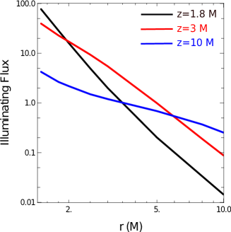
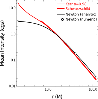
Figure 2: Left: Illuminating flux, $\mathcal{F}(r)$, as defined in Eq. 2 for a spectral index $\alpha=1$ and three different altitudes of the lamp, $z=1.8\,M$ (magenta), $z=3\,M$ (red) and $z=10\,M$ (blue). Radius is in $M$ units and flux in arbitrary units. This figure is extremely similar to Fig. 2, lower panel, of Dauser et al. (2013). Right: Illuminating mean intensity in cgs units, $\mathcal{I}(r)$, computed in a Newtonian spacetime (solid black and circles), a Schwarzschild spacetime (thick red) and a Kerr spacetime with spin parameter $a=0.98$ (thin red). The black circles are Newtonian illuminating fluxes as computed by GYOTO while the solid black line is the analytical expression of the Newtonian mean intensity.

We are able to compute precisely illuminating fluxes or mean intensities for any kind of lamp position and geometry. We are also able to consider either a black-hole metric, or flat spacetime in order to compare Newtonian and general-relativistic (GR) illuminating fluxes or mean intensities. Newtonian illuminating mean intensities are computed by assuming a Minkowski metric, an observer at rest at coordinate radius $r$, and fixing to $g=1$ the redshift factor (in order to remove all relativistic effects including special relativistic effects that would still be present in a Minkowski spacetime if $g$ is not fixed to $1$).

At this stage, we only need to define the normalizing constant $A$ in order to compute mean intensities $\mathcal{I}(r)$ in cgs units. We do this by choosing one particular value of the total X-ray luminosity illuminating an accretion disk. This total luminosity can be written

$$L_{X,\mathrm{illum}}=2\int_{\nu_{\mathrm{lamp}}\in X}\int_{\mathcal{S}_{\mathrm{disk}}}F^{\mathrm{disk}}_{\nu}(r)\mathrm{d}S_{\mathrm{disk}}(r)\mathrm{d}\nu_{\mathrm{disk}}(r)$$ (5)

where $\nu_{\mathrm{lamp}}$ is the lamp-frame frequency which is varied in the X band between $\nu_{\mathrm{lamp,1}}$ and $\nu_{\mathrm{lamp,2}}$, $\nu_{\mathrm{disk}}(r)$ is the corresponding redshifted frequency at radius $r$ in the disk frame, and $\mathrm{d}S_{\mathrm{disk}}(r)$ is the infinitesimal disk area between $r$ and $r+\mathrm{d}r$ in the disk frame. The factor of $2$ in this expression is justified by considering a symmetric source, illuminating both sides of the disk. We note that our numerical treatment only considers illumination from one side of the disk. However, in a realistic situation (for instance if the source is the base of a jet), this illuminating source should be present on both sides of he disk. The luminosity $L_{X,\mathrm{illum}}$ above is defined in order to normalize all quantities to realistic values. As a consequence, it should contain this factor of $2$. Considering two symmetric sources in the numerical treatment would not change anything because the observer will always see only one side of the disk (neglecting the small contribution of the very gravitationally bent radiation coming from the lower side that can be seen from the upper side of the disk). In the Kerr metric, the redshift factor $g$ is known analytically so that we may write in the equatorial plane

$$\nu_{\mathrm{disk}}(r)=\nu_{\mathrm{lamp}}\frac{r^{3/2}+a}{\sqrt{r^{3}+2ar^{3/2}-3r^{2}}}\sqrt{\frac{z^{2}+a^{2}-2z}{z^{2}+a^{2}}}$$ (6)

where $a$ is the black hole spin parameter. The element of area in the equatorial plane is

$$\mathrm{d}S_{\mathrm{disk}}(r) = \sqrt{g_{rr}g_{\varphi\varphi}}\mathrm{d}r\mathrm{d}\varphi$$

$$= 2\pi r\sqrt{\frac{r^{2}+a^{2}+2a^{2}/r}{r^{2}-2r+a^{2}}}\mathrm{d}r$$

where $g_{rr}$ and $g_{\varphi\varphi}$ are Kerr metric coefficients. The total illuminating luminosity is thus

$$L_{X,\mathrm{illum}} = 2A\frac{\nu_{\mathrm{lamp,2}}^{1-\alpha}-\nu_{\mathrm{lamp,1}}^{1-\alpha}}{1-\alpha}$$

$$\times\int_{r_{\mathrm{min}}}^{r_{\mathrm{max}}}\mathcal{F}(r)2\pi r\sqrt{\frac{r^{2}+a^{2}+2a^{2}/r}{r^{2}-2r+a^{2}}}$$

$$\times\left(\frac{r^{3/2}+a}{\sqrt{r^{3}+2ar^{3/2}-3r^{2}}}\sqrt{\frac{z^{2}+a^{2}-2z}{z^{2}+a^{2}}}\right)^{1-\alpha}\mathrm{d}r$$

which can be integrated numerically. Here, $r_{\mathrm{min}}$ and $r_{\mathrm{max}}$ are the inner and outer radii of the accretion disk. Thus, by choosing $L_{X,\mathrm{illum}}$, the normalizing constant $A$ is known. We note that this normalization depends on the spin parameter. In order to consider one common lamp for all simulations presented in this work, we choose to normalize the problem for $a=0$ and to use the same normalization whatever the spin. This means that $L_{X,\mathrm{illum}}$ will not be the same for different spins, it is rather the lamp which is kept the same for all simulations.

For a spin-0 black hole, we consider a luminosity of $L_{X,\mathrm{illum}}(a=0)=10^{36}\,\mathrm{erg}\,\mathrm{s}^{-1}$. This choice fixes the normalizing constant $A$, which is kept the same for both $a=0$ and $a=0.98$. The corresponding illuminating luminosity for $a=0.98$ is $L_{X,\mathrm{illum}}(a=0.98)=1.3\times 10^{36}\,\mathrm{erg}\,\mathrm{s}^{-1}$. We note that the accretion-related luminosity is equal $L_{X,\mathrm{acc}}=2\times 10^{37}\,\mathrm{erg}\,\mathrm{s}^{-1}$ with our choice of accretion rate and taking an accretion efficiency of $\eta=0.1$. This means that the accretion luminosity is bigger than the illumination by an order of magnitude. Consequently, we are modeling a thermally dominated state with a weak hard tail (for a review on X-ray binaries states and radiative processes, see Zdziarski & Gierliński 2004).

We keep constant the following parameters: $z=10\,M$, $\alpha=0.7$, $h\nu_{\mathrm{lamp,1}}=2$ eV and $h\nu_{\mathrm{lamp,2}}=10^{5}$ eV. All these fixed parameters are also given in Table 1. In particular, we will not vary the lamp height $z$ although this parameter has an important impact on the illumination (see e.g. Dauser et al. 2013). Our goal here is not to scan the full parameter space but rather to determine the effect of the spin parameter on the reflected spectrum in a setup where the lamp is sufficiently close to the black hole to lead to non-negligible light-bending effects.

Table 1: Lamp post model fixed parameters used in this article.

Parameter	Notation	Value
Black hole mass	$M$	$10\,M_{\odot}$
Accretion rate	$\dot{m}$	$0.01\,\dot{m}_{\mathrm{Edd}}$
Lamp height	$z$	$10\,M$
Spectral index	$\alpha$	$0.7$
Disk inner radius	$r_{\mathrm{min}}$	$7M(a=0)/2M(a=0.98)$
Disk outer radius	$r_{\mathrm{max}}$	$120\,M$
Illumination bounds	$h\nu_{\mathrm{lamp}}$	[2 eV ; $10^{5}$ eV]

The resulting mean intensities in cgs units, considering Newtonian, Schwarzschild and close-to-extreme Kerr spacetimes are presented in Fig. 2, right panel. This Figure in particular shows a comparison between the GYOTO-computed Newtonian mean intensity and its analytical expression

$$\mathcal{I}_{\mathrm{Newton}}\propto\frac{1}{r^{2}+z^{2}}.$$ (9)

The agreement is within $\approx 0.2\%$. We note that even at large distances, the illuminating relativistic mean intensities differ (by roughly $25\,\%$) from the Newtonian ones. This can be understood by noticing that even when the Keplerian observer is at a large distance, the illuminating radiation is always emitted in the strong gravitational field region and thus always contains a relativistic signature.

At this stage, we are ready to compute the reflected spectrum due to the reprocessing of the lamp radiation by the disk. We will consider an illuminating mean intensity as computed in a Newtonian spacetime, or in a Kerr spacetime with spin parameter $a=0$ or $a=0.98$.

3 Reflected spectra

3.1 Local spectra

Local spectra are computed using the radiative transfer code ATM21 as described in Różańska et al. (2011). We refer to this paper, as well as to Madej & Różańska (2004) and Różańska & Madej (2008), for more details and will give here only the most important steps. We stress that ATM21 computes simultaneously the structure of an irradiated atmosphere and its outgoing line and continuum spectrum, the atmosphere being both in hydrostatic and radiative equilibrium.

Our radiative transfer equation assumes a plane-parallel geometry and reads

$$\mu\frac{\mathrm{d}I_{\nu}}{\mathrm{d}\tau_{\nu}}=I_{\nu}-\frac{j_{\nu}}{\kappa_{\nu}+\sigma_{\nu}}$$ (10)

where $\mu=\cos i$ is the cosine of the angle between the light ray and the local normal, $j_{\nu}$ is the emissivity, $\kappa_{\nu}$ is the opacity, $\sigma_{\nu}$ is the scattering coefficient, and $\mathrm{d}\tau_{\nu}=-(\kappa_{\nu}+\sigma_{\nu})\rho\,\mathrm{d}z$, where $\rho$ is the mass density, is the optical depth. Emissivity takes into account the disk thermal emission, Compton scattering redistribution functions and iron fluorescence lines from the gas at each ionization state.

In our numerical procedure, the equation above is solved with the structure of the gas kept in radiative, hydrostatic and ionization equilibrium. We use local thermal equilibrium (LTE) absorption $\kappa_{\nu}$, whereas coefficients of emission $j_{\nu}$ and scattering $\sigma_{\nu}$ include non-LTE terms. The coefficient of true absorption considers photoionization from numerous levels of atoms and ions as well as Bremsstrahlung (free-free) absorption from all ions.

The external illumination by X-ray photons is fully taken into account as an additional intensity field which enters the atmosphere from above. This energy-dependent radiation modifies the temperature and the gas ionization level in addition to the disk thermal radiation generated below the atmosphere via viscosity mechanism.

Both radiation intensities are scattered by Compton process, which is included in the radiative transfer equation using angle-averaged Compton redistribution functions (after Pomraning 1973; Guilbert 1981; Kershaw 1987). Compton scattering cross-sections were computed following the paper by Guilbert (1981), corrected for computational errors in the original paper (see Madej et al. 2016), and for the first time presented in a computer code by Madej (1989). Our equations and the Compton redistribution functions work correctly in cases of both large and small energy exchange between X-ray photons and free electrons at the time of scattering. They ensure accurate solution of the radiative transfer also in cases when the initial photon energy before or after scattering exceeds the electron rest mass ($m_{\rm e}c^{2}=511$ keV).

We highlight that we compute the full reflected spectra, meaning that we take into account both the thermal component emitted by the accretion disk at the local temperature and the reflected part due to the reprocessing of the light emitted by the lamp. Therefore, the disk emission and X-ray illumination always self-consistently influence the matter thermal and ionization structure. As a result, the outgoing local spectrum contains all reprocessing signatures, such as: the deviation of the thermal spectrum from pure blackbody due to photo-absorption and re-emission, the deviation of the spectrum due to photon energy shift by Compton scattering, the Compton hump due to the reflection from the heated atmosphere (both effects are presented in Madej & Różańska 2000), and the fluorescent iron line complex (Różańska & Madej 2008; Różańska et al. 2011).

3.1.1 Computing local spectra

We model the accretion disk by a stationary relativistic slim disk solution (Sa̧dowski et al. 2011), which depends on the black hole mass and assumed accretion rate, assumed here to be: $M=10$ M_⊙ and $\dot{m}=0.01\,\dot{m}_{\mathrm{Edd}}$. This allows to compute the vertical gravity and effective temperature radial distributions that are input parameters of our radiative transfer computations. These quantities depend on the spin parameter, which is thus taken into account self-consistently. From those quantities, the radiative transfer is solved for a set of discretized radii, assuming that the disk has solar-like chemical abundances. At each radius, vertical gravity and effective temperature are only needed to formulate the boundary conditions of the vertical atmosphere’s structure. Subsequent iterations proceed between the radiation field and the gas structure, as it should be when solving radiation transfer problem. For the atmosphere, we assume hydrostatic and radiative equilibrium, which adds an additional differential equation to the whole problem, making the derivation of the solution much more complex and time consuming than in the case of a constant-density gas (as done in García et al. 2014).

The Fe $K\alpha$ doublet fluorescence lines are set to central energies from $6.404$ keV and $6.391$ keV to $6.652$ keV and $6.639$ keV, depending on the matter ionization level. The iron $K\beta$ line energy centroid is $7.057$ keV. Their natural widths are set respectively to $2.7$ eV, $3.3$ eV and $2.5$ eV. The boundary condition of the radiative transfer equation is set by the illumination mean intensity profile computed in Section 2 which gives the value of the mean intensity for all radii and the associated direction cosine $\mu_{\mathrm{illum}}$. Deep in the disk atmosphere, we assume full thermalization. Nevertheless, in our scheme when iterating between the gas structure and the radiation field at each point of the atmosphere, including the deepest one, temperature corrections are taken into account.

The radiative transfer equation is solved for a set of $\approx 30$ radial points, $8$ directional cosines $\mu$ between $0.02$ and $0.98$ and for $\approx 2600$ values of photon energy between $2$ eV and $10^{5}$ eV. The precise definition of the grids considered for the two spin values we take into account is given in Table 2. The output of this Section is the value of the reprocessed specific intensity $I_{\nu}^{\mathrm{repro}}$ as a function of the $8$ direction cosines $\mu$ and of the $\approx 2600$ photon energies, for all values of radii in the disk where the radiative transfer is solved. This final reprocessed intensity consists in both the thermal emission from the cold accretion disk and the mixture of absorbed and then re-emited radiation, either by true absorption or scattering, outgoing from the hot skin.

Table 2: Local spectra are computed at $n_{r}$ radial points chosen between $r_{\mathrm{min}}(a)$ and $r_{\mathrm{max}}$, where $a$ is the spin parameter. The radial grid is denser close to $r_{\mathrm{min}}$ and becomes more sparse as $r$ increases. When two values are given separated by a $"/"$ sign, the first one is used for $a=0$ and the second one for $a=0.98$. The ISCO radius for both spins are $r_{\mathrm{ISCO}}(a=0)=6\,M$ and $r_{\mathrm{ISCO}}(a=0.98)=1.6\,M$. The smallest radial value is always chosen slightly above the ISCO. The grid contains $n_{i}$ direction cosines $\cos i$ and $n_{E}$ photon energies.

$r_{\mathrm{min}},r_{\mathrm{max}},n_{r}$	$7M/2M,\,120M,\,31/36$
$n_{i}$	$8$
$\cos i$	$(0.02,0.1,0.2,0.4,0.6,0.75,0.9,0.98)$
$n_{E}$	$2600$

3.1.2 Dependence on illumination computation, spin and direction

Fig. 3 illustrates the effect of changing the computation of the illumination (Newtonian or GR) and the value of spin on the local spectrum. As illustrated in the upper left panel, the spectrum is made of three parts:

• the thermal bump (around $100\,\mathrm{eV}-1\,\mathrm{keV}$) is due to two forms of dissipation: viscous dissipation in the accretion disk and heating by the irradiation of the lamp. However for our choice of parameter, the viscous heating is dominating (see the end of Section 2);

• the iron-line complex due to fluorescent emission (around $6.4$ keV);

• and the Compton hump (at energies just above the iron-line complex) due to the Compton back scattering of hard photons.

The thermal part of the spectrum will be less affected by changing the illumination as part of it is computed from the hydrostatic equilibrium temperature of the accretion disk which only slightly depends on illumination. The reflected part of the spectrum (iron-line complex plus Compton hump) depends on the illumination profile considered. At small radii, the reflected spectrum is stronger for GR illumination, while at bigger radii, the opposite is true and the Newtonian illumination leads to a stronger reflected spectrum. This is in perfect agreement with Fig. 2, right panel, which shows that the Newtonian illumination dominates the general-relativistic one at big radii, while it is smaller at small radii, because of light bending effect.

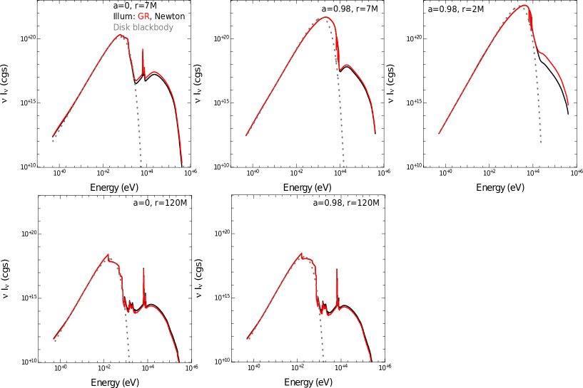
Figure 3: Local $\nu I_{\nu}$ spectra: impact of illumination computation (Newtonian or GR) and spin. Only one direction cosine is considered, $\cos i=0.98$ (almost face-on, i.e. close to the normal to the disk). The illumination is computed in general relativity (red) or in a Newtonian spacetime (black). The grey dotted spectrum is the blackbody function at the local temperature. The spin is $0$ is the left column and $0.98$ in the right column. The spectrum is computed at $r=2M$ (upper row, right panel), $r=7M$ (upper row left and middle panels) or $r=120M$ (lower row).

Fig. 4 shows the relative difference $\mathcal{R}$ between the local spectra computed with a Newtonian or GR illumination, at the inner disk radius (where most of the radiation is emitted). It is computed following

$$\mathcal{R}=200\frac{\mathrm{spectrum\,GR}-\mathrm{spectrum\,Newton}}{\mathrm{spectrum\,GR}+\mathrm{spectrum\,Newton}}.$$ (11)

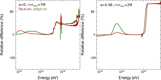
Figure 4: Local $\nu I_{\nu}$ spectra: relative difference at $r_{\mathrm{min}}$ for GR/Newtonian illuminations. The red curve shows the relative difference between the local spectrum computed with GR or Newtonian illuminations in the face-on direction. The green curve shows the same quantity for the edge-on direction. Spin is $0$ on the left panel and $0.98$ on the right panel. The spectrum is computed in both cases at $r=r_{\mathrm{min}}$.

Fig. 3 also shows the influence of the spin parameter on the local spectrum. Higher spin leads to higher disk temperature (see Fig. 1 of Różańska et al. 2011), particularly at smaller radii (the spin dependence decreases to zero as $r$ increases). As a consequence, at $r=7M$, the thermal bump peaks higher and so does the Compton hump as Comptonization is depending on the disk temperature. At $r=120M$ the spectra are very similar for $a=0$ and $a=0.98$, as they should be. The thermal bump for spin $a=0.98$ deviates from blackbody radiation since for the inner regions the disk effective temperature is high. Such an atmosphere is made of an almost completely ionized gas allowing for efficient Compton scattering. This modifies the high energy tail and the frequency of peak flux of thermal radiation as demonstrated in Madej (1991). The outgoing spectrum is sensitive to the local vertical temperature and ionization structure. Therefore, spectra emerging from the outer radii at r=120 M for both spins may sligthly differ, since reprocessing depends on many aspects like the exact illumination field and the detailed vertical structure. The appearance of spectral features also depends on local thermodynamical conditions. If the external illumination is low in comparison to the disk temperature, we clearly see ionization edges in absorption. But when the illumination increases, many spectral features start to be visible in emission as shown by Madej & Różańska (2000). When matter is completely ionized we do not see any spectral features in the reflected part of the spectrum. Finally, if the inner disk temperature is high enough, thermal radiation modified by Compton scattering covers the iron line region, and this feature is only visible as the resonant line in absorption from the hot atmosphere (Różańska et al. 2011). This result clearly shows that properly computed disk thermal component should be taken into account in the models used for spin fitting from iron line shape in black hole binaries.

Fig. 5 illustrates the dependence on the direction of the local spectrum. For both spins, edge-on ($\cos i=0.02$) emission is smaller in the thermal bump but higher in the reflected part of the spectrum. This is of course in agreement with the discussion in Różańska et al. (2011) as we are using the same model (but using a denser radial grid), with only a differing illumination. It is interesting to note two more things. First, for both spins, the reflected part of the spectrum is more and more depending on direction as the radius gets bigger. Second, at small radii, the reflected spectrum is much less dependent on direction for higher spin than for lower spin. This is because the gas on innermost rings is hot itself and the thermal spectrum covers flat part of reflected spectrum. We see only steep part of the refleced spectrum which does not depend much on the direction.

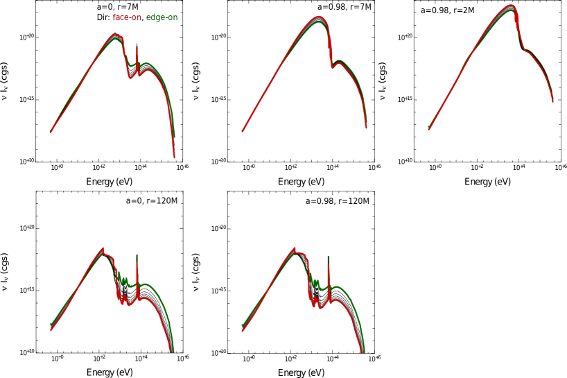
Figure 5: Local $\nu I_{\nu}$ spectra: impact of direction. The illumination is computed in general relativity. The spectrum is computed at $r=7M$ (top row) and $r=120M$ (bottom row). The spin is $0$ (left panel) or $0.98$ (right panel). All $8$ direction cosines $\cos i$ given in Table 2 are represented with almost face-on reflected spectrum ($\cos i=0.98$) in red and edge-on ($\cos i=0.02$) in green.

3.2 Ray tracing observed spectra

At this point we are ready to start the third and last step of our numerical pipeline, which is the ray tracing of the reflected spectrum to a distant observer.

The main aim of this section is to analyze the importance of taking into account the directional dependence (as a function of $\mu$) of the local spectrum in order to compute observed spectra. We note that we will often use in this section the expression observed spectrum having in mind the reprocessed (thermal+reflected) spectrum ray traced to infinity. The direct component is shown separately to briefly discuss the relative strength of the reprocessed/direct components, but we mainly focus in the following on the reprocessed part. This is the same analysis as already done by García et al. (2014), but with the important distinction of using a very different code for computing the local spectrum.

Photons are ray traced backwards in time from an observer located at $r=10^{10}\,M$. When a photon hits the accretion disk at radius $r$, the disk-frame frequency $\nu$ and direction cosine $\mu$ are determined. This last quantity is readily computed knowing the 4-velocity of the emitting gas $\mathbf{u}$, the 4-vector tangent to the emitted photon geodesic $\mathbf{p}$ and the local disk normal 4-vector $\mathbf{n}$

$$\mu=-\frac{\mathbf{n}\cdot\mathbf{p}}{\mathbf{u}\cdot\mathbf{p}}.$$ (12)

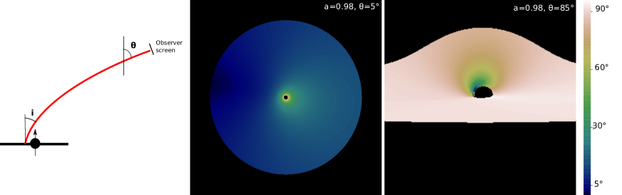
Figure 6: Map of emission angle for spin $a=0.98$. Left: geometry of the problem with the inclination angle $\theta$ between the black-hole spin axis and the line of sight, and the emission angle $i$ between the disk normal and the direction of emission of the photon in the emitter’s frame. Center and Right: these maps show a map of the values of the emission angle $i$ between the local normal to the accretion disk and the direction of photon emission for a spin of $a=0.98$. The inclination angle is equal $\theta=5^{\circ}$ (center) or $\theta=85^{\circ}$ (right). The right panel can be compared to Fig. 5, lower left panel of García et al. (2014).

Fig. 6 shows the distribution of the emission angle $i$ (such as $\mu=\cos i$) in a disk surrounding an extreme Kerr black hole seen under two different inclinations, $\theta=5^{\circ}$ and $\theta=85^{\circ}$. Strong bending of light rays in the central region of spacetime leads to a large set of emission angles being present for one given value of the inclination $\theta$, in contrast to a Newtonian spacetime for which $i=\theta$. From this Figure only it is clear that considering an emission-angle-averaged or a directional emission may lead to very different observed spectra. It is the aim of this Section to investigate this question, following the previous analysis by García et al. (2014).

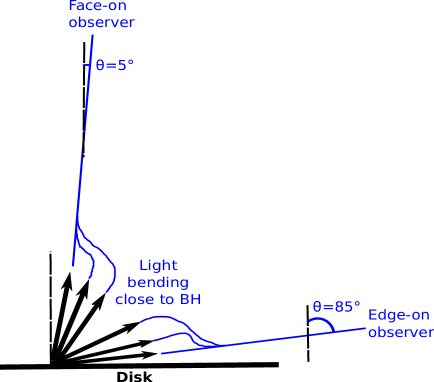
Figure 7: Illustrating the angle dependence of ray-traced spectra. Ray-traced spectra in this article are computed from two inclination angles, $\theta=5^{\circ}$ (face-on observer) or $\theta=85^{\circ}$ (edge-on observer). From each of this inclination angles, photons are ray traced backwards to the accretion disk (blue lines). For one given inclination $\theta$, photons reach the disk with a set of different directions because of light bending. This is illustrated in the Figure by the fact that one given blue line is connected to a set of different directions of local emission in the disk (black arrows, the black vertical dashed line being the local normal). This means that the face-on observer, e.g., sees photons emitted not only at face-on emission but also in all other emission directions. Directional ray-traced spectra are computed by transporting along each geodesic the specific intensity $I_{\nu}(r,i)$ emitted at the local position $r$ in the direction $i$ of this particular geodesic. Angle-averaged ray-traced spectra are computed by transporting along each geodesic the angle-averaged specific intensity $I_{\nu}(r)$ obtained by averaging $I_{\nu}(r,i)$ over all emission angles $i$.

Fig. 7 illustrates the various angles used in our analysis and defines in more detail the notion of angle-averaged ray-traced spectrum. When a backwards-in-time ray-traced photon hits the disk, and after having computed the emitted frequency $\nu$ and the direction cosine $\mu$, the specific intensity $I_{\nu}^{\mathrm{repro}}(r,\mu,\nu)$ is trilinearly interpolated (i.e. linearly in all 3 dimensions) from the results of Section 3.1. For computing an angle-averaged spectrum, this quantity is simply averaged over the direction cosine $\mu$

$$I_{\nu}^{\mathrm{repro,avg}}(r,\nu)=\int I_{\nu}^{\mathrm{repro}}(r,\mu,\nu)\mathrm{d}\mu.$$ (13)

The specific intensity in the distant observer’s frame $I_{\nu}^{\mathrm{obs}}$ is then deduced by using the frame invariance of $I_{\nu}/\nu^{3}$. Thus a map of specific intensity in the observer’s frame (i.e. an image of the disk) can be computed, which is readily transformed to a flux value by summing over all directions on sky. The observed spectrum is thus at hand.

Fig. 8 shows the angle-averaged and directional ray-traced spectra for both spins, together with their relative difference. This Figure also shows the level of the direct-component power law, directly reaching the observer from the lamp. This component was computed by ray tracing the lamp alone, as observed by the distant observer, and keeping the same normalization of the emitted intensity as described in Section 2. It shows that our choice of parameters leads to a total spectrum dominated by the direct and thermal components.

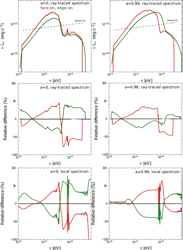
Figure 8: Ray-traced $\nu L_{\nu}$ spectra: impact of directionality. The local spectra have been computed with GR illumination. The top row shows emission-angle-averaged (dotted) and angle-dependent (solid) ray-traced spectra. The straight black dashed line shows the level of the direct-component power law (see text for details). The middle row shows the relative difference between averaged and angle-dependent ray-traced spectra. The bottom row shows the same quantity as the middle row for the local spectra, evaluated at $r=r_{\mathrm{min}}$. The spin is $0$ (left column) or $0.98$ (right column). Red curves refer to spectra ray traced from an inclination of $\theta=5^{\circ}$, i.e. close to face-on. Green curves are computed at an inclination of $\theta=85^{\circ}$, i.e. close to edge-on. Note that ”face-on” and ”edge-on” in the two upper rows (ray-traced quantities) refer to the inclination angle $\theta$, while in the bottom row (local quantities) these words refer to the emission angle $i$.

Fig. 8 also shows the relative difference between the directional and angle-averaged local (non-ray-traced) spectra, computed for both spins at $r=r_{\mathrm{min}}$. This Figure shows a few important things. As we will discuss this quantity a lot, let us call $\mathcal{R}$ the relative difference between angle-averaged and directional spectra, which is computed in the same way as in Eq. 11. First, $\mathcal{R}$ can go as high as $\approx 70\%$, and in particular in the region of the iron-line complex it is of the order of $50\%$. This maximum value of $\mathcal{R}$ is the same for local and ray-traced spectra. The general behavior of $\mathcal{R}$ is rather similar for local and ray-traced spectra. However, there is an important difference: the edge-on value of $\mathcal{R}$ is always significantly smaller than its face-on value for ray-traced spectra (particularly at high spin), while for local spectra the difference is less pronounced. This means that edge-on ray-traced spectra are closer to the angle-averaged spectra than face-on ray-traced spectra. This fact can be understood as follows.

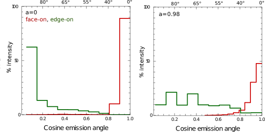
Figure 9: Specific intensity distribution with emission angle. This Figure shows the histogram of specific intensity emitted at the disk’s surface in percent of the total intensity as a function of $\cos i$. This total intensity is defined simply as the sum of the specific intensity map over all pixels. It is thus proportional to the total observed flux. The spin is $0$ on the left, $0.98$ on the right. The inclination is face-on in red, edge-on in green.

Fig. 9 shows the observed specific intensity distribution as a function of the direction cosine $\mu$, for both spins. It shows that photons forming the face-on ray-traced spectrum are emitted in a narrower range of values of $\mu$ than their edge-on counterparts. This effect gets stronger with increasing spin: for $a=0.98$, photons forming the edge-on ray-traced spectrum are coming from a very broad range of values of $\mu$. This explains why edge-on ray-traced spectra are closer to the angle-averaged solution, and even more at higher spins. The strong dependence on the spin parameter of this effect is explained

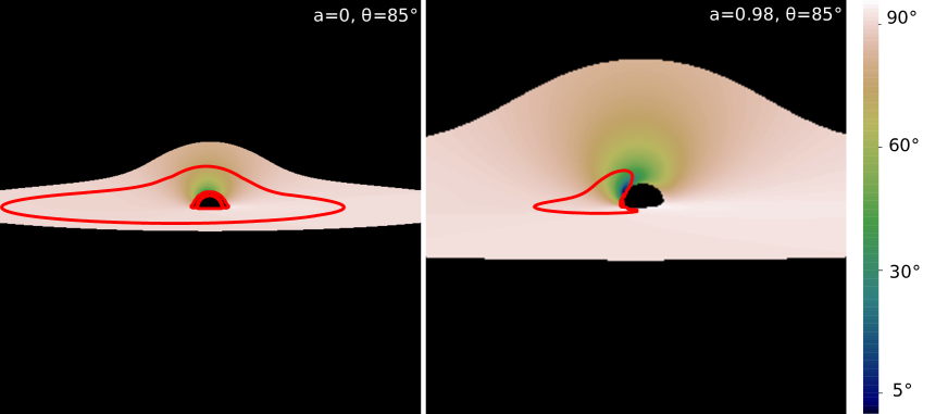
Figure 10: Angle map and intensity contour for edge-on inclination. The two panels show a map of the values of the emission angle $i$ for both spins at edge-on inclination. Over-plotted is one specific intensity contour in red, encompassing $90\%$ of the total specific intensity emitted at the disk’s surface. The beaming effect is already clear at spin zero: more intensity is emitted on the left part of the image where matter moves towards the observer. The beaming effect is extremely strong at high spin, only a very small part of the disk emits most of the radiation observed.

in Fig. 10. This Figure shows that the very strong relativistic beaming effect at high spin has for consequence that most of the flux is emitted from the very inner parts of the disk, where the emission angle $i$ varies a lot (see Fig. 6, right panel). Thus, all possible values of emission angle contribute and the final spectrum is closer to the averaged solution.

As far as the emission-angle-dependence of the spectra are concerned, our results are in reasonable agreement with the findings of García et al. (2014). Our Fig. 9, right panel, can be compared to Fig. 8, upper-right and lower-right panels of García et al. (2014), which are similar. This shows once again that the ray-tracing part of the computation is very similar in both works. It is more complicated to go into a detailed comparison of the observed spectra and their dependence on the emission angle $i$. Our Fig. 8 is different from the left panels of Fig. 8 of García et al. (2014), and this is obviously due to the differences in the computation of local spectra. García et al. (2014) find a maximum difference between directional and angle-averaged spectra of $\gtrsim 20\%$ (taking into account their results for $z=10\,M$ only of course), while we find a maximum difference of up to $50\%$. It is not possible to go further in the comparison without doing a complete code comparison, which is not the aim of this paper. Still, the conclusions of both completely independent treatments are reasonably similar, as far as the angle dependence of the spectra is concerned.

The upper-right panel of Fig. 8 shows no iron line for $a=0.98$, neither in emission nor in absorption. This was already noticeable in the upper middle and right panels of Fig. 5 showing the local spectra that exhibit very narrow absorption lines due to the fact that the thermal bump covers the iron-line complex. The relativistic blurring of these narrow lines has for consequence to completely remove the line from the observed spectrum. However, the fact that the thermal bump covers the iron-line complex is due to our choice of parameters for which the illumination luminosity is dominated by the accretion-induced luminosity. We have checked that for a much smaller accretion rate ($\dot{m}=10^{-5}\,m_{\mathrm{Edd}}$ ; with the same illumination) the local spectrum at spin $0.98$ has a less prominent thermal bump leading to a clear iron line in emission, similarly to the $a=0$ case depicted in Fig. 5. This fact shows that a detailed study of the observed iron-line complex as a function of the ratio of the illuminating to accretion-induced luminosities would be very interesting. Such an analysis goes beyond the scope of the present paper and we will present it in a future article.

The conclusion of this Section is that it is very important to take into account the directionality of the emitted, local spectrum in order to predict the iron-line complex of the observed spectrum. Indeed, the error on the observed spectrum caused by angle averaging is as high as $50\%$ in the iron line region.

4 Conclusion

The aim of this article is to compute X-ray spectra reprocessed by the accretion disk of an X-ray binary in a very realistic way. We consider the isotropic emission of X-rays from a nearly point-like lamp at rest at $z=10\,M$ along the black hole axis. We have computed in full general relativity the irradiation onto the accretion disk for two extreme values of the spin parameter $a=0$ and $a=0.98$. We then compute the local spectra reprocessed by the accretion disk, taking self-consistently into account the black spin by solving the hydrostatic equilibrium of the disk together with the radiative transfer. Finally we ray trace this local spectrum to a distant observer in order predict a very realistic observed spectrum.

We show that taking into account the angle dependence of the local spectra is very important for obtaining an accurate observed spectrum. In particular, the influence of averaging out the angular information of the local spectra leads to an error in the observed spectrum of $50\%$ in the iron-line region, which is the important region to constrain black hole spins.

We also show that, for the set of parameters chosen in this work, the disk thermal emission is strong enough to cover the iron line complex for spin $a=0.98$, resulting in a featureless reflected spectrum. On the other hand, the direct component is much higher than the reflected one at a=0. Thus, for both spins, the observed (direct+thermal+reflected) spectrum contains only weak reflection features.

We intend to devote future work to investigating in detail the appearance of the observed spectrum in various X-ray binary states (thermal dominated and hard state) for a set of different lamp altitudes (which has a strong impact on the reprocessed/direct components ratio). This will allow us to determine what sets of parameters allow to generate reflection-dominated spectra for different source spectral states.

References

- Ballantyne et al. (2001) Ballantyne, D. R., Ross, R. R., & Fabian, A. C. 2001, MNRAS, 327, 10
- Czerny & Zycki (1994) Czerny, B. & Zycki, P. T. 1994, ApJ, 431, L5
- Dauser et al. (2013) Dauser, T., Garcia, J., Wilms, J., et al. 2013, MNRAS, 430, 1694
- Done et al. (2007) Done, C., Gierliński, M., & Kubota, A. 2007, A&A Rev., 15, 1
- Dovciak & Done (2015) Dovciak, M. & Done, C. 2015, in The Extremes of Black Hole Accretion, 26
- Dovciak et al. (2013) Dovciak, M., Matt, G., Bianchi, S., et al. 2013, ArXiv e-prints
- Dovciak et al. (2014) Dovciak, M., Svoboda, J., Goosmann, R. W., et al. 2014, ArXiv e-prints
- Fabian et al. (1989) Fabian, A. C., Rees, M. J., Stella, L., & White, N. E. 1989, MNRAS, 238, 729
- Fukumura & Kazanas (2007) Fukumura, K. & Kazanas, D. 2007, ApJ, 664, 14
- García et al. (2014) García, J., Dauser, T., Lohfink, A., et al. 2014, ApJ, 782, 76
- García & Kallman (2010) García, J. & Kallman, T. R. 2010, ApJ, 718, 695
- George & Fabian (1991) George, I. M. & Fabian, A. C. 1991, MNRAS, 249, 352
- Guilbert (1981) Guilbert, P. W. 1981, MNRAS, 197, 451
- Haardt & Maraschi (1991) Haardt, F. & Maraschi, L. 1991, ApJ, 380, L51
- Kershaw (1987) Kershaw, D. S. 1987, J. Quant. Spec. Radiat. Transf., 38, 347
- Madej (1989) Madej, J. 1989, ApJ, 339, 386
- Madej (1991) Madej, J. 1991, ApJ, 376, 161
- Madej & Różańska (2000) Madej, J. & Różańska, A. 2000, A&A, 363, 1055
- Madej & Różańska (2004) Madej, J. & Różańska, A. 2004, MNRAS, 347, 1266
- Madej et al. (2016) Madej, J., Różańska, A., Majczyna, A., & Należyty, M. 2016, ArXiv e-prints 1602.05088
- Magdziarz & Zdziarski (1995) Magdziarz, P. & Zdziarski, A. A. 1995, MNRAS, 273, 837
- Markoff et al. (2005) Markoff, S., Nowak, M. A., & Wilms, J. 2005, ApJ, 635, 1203
- Martocchia & Matt (1996) Martocchia, A. & Matt, G. 1996, MNRAS, 282, L53
- Matt et al. (1991) Matt, G., Perola, G. C., & Piro, L. 1991, A&A, 247, 25
- Miller et al. (2014) Miller, J. M., Mineshige, S., Kubota, A., et al. 2014, ArXiv e-prints 1412.1173
- Miniutti & Fabian (2004) Miniutti, G. & Fabian, A. C. 2004, MNRAS, 349, 1435
- Miniutti et al. (2003) Miniutti, G., Fabian, A. C., Goyder, R., & Lasenby, A. N. 2003, MNRAS, 344, L22
- Nandra et al. (2013) Nandra, K., Barret, D., Barcons, X., et al. 2013, ArXiv e-prints
- Nayakshin & Kallman (2001) Nayakshin, S. & Kallman, T. R. 2001, ApJ, 546, 406
- Niedźwiecki et al. (2016) Niedźwiecki, A., Zdziarski, A. A., & Szanecki, M. 2016, ApJL, in press, ArXiv e-prints 1602.09075
- Niedźwiecki & Życki (2008) Niedźwiecki, A. & Życki, P. T. 2008, MNRAS, 386, 759
- Pomraning (1973) Pomraning, G. C. 1973, The equations of radiation hydrodynamics
- Poutanen et al. (1996) Poutanen, J., Nagendra, K. N., & Svensson, R. 1996, MNRAS, 283, 892
- Reynolds et al. (2014) Reynolds, C., Ueda, Y., Awaki, H., et al. 2014, ArXiv e-prints 1412.1177
- Reynolds (2014) Reynolds, C. S. 2014, Space Sci. Rev., 183, 277
- Reynolds & Nowak (2003) Reynolds, C. S. & Nowak, M. A. 2003, Phys. Rep, 377, 389
- Reynolds et al. (1999) Reynolds, C. S., Young, A. J., Begelman, M. C., & Fabian, A. C. 1999, ApJ, 514, 164
- Ross & Fabian (1993) Ross, R. R. & Fabian, A. C. 1993, MNRAS, 261, 74
- Różańska et al. (2002) Różańska, A., Dumont, A.-M., Czerny, B., & Collin, S. 2002, MNRAS, 332, 799
- Różańska & Madej (2008) Różańska, A. & Madej, J. 2008, MNRAS, 386, 1872
- Różańska et al. (2011) Różańska, A., Madej, J., Konorski, P., & Sa̧dowski, A. 2011, A&A, 527, A47
- Ruszkowski (2000) Ruszkowski, M. 2000, MNRAS, 315, 1
- Sa̧dowski et al. (2011) Sa̧dowski, A., Abramowicz, M., Bursa, M., et al. 2011, A&A, 527, A17
- Takahashi et al. (2014) Takahashi, T., Mitsuda, K., Kelley, R., et al. 2014, ArXiv e-prints 1412.2351
- Vincent et al. (2011) Vincent, F. H., Paumard, T., Gourgoulhon, E., & Perrin, G. 2011, Classical and Quantum Gravity, 28, 225011
- Wilkins & Fabian (2012) Wilkins, D. R. & Fabian, A. C. 2012, MNRAS, 424, 1284
- Zdziarski & Gierliński (2004) Zdziarski, A. A. & Gierliński, M. 2004, Progress of Theoretical Physics Supplement, 155, 99
- Zycki & Czerny (1994) Zycki, P. T. & Czerny, B. 1994, MNRAS, 266, 653