Phase diagram of the two-fluid Lipkin model: a butterfly catastrophe

Abstract

Background:

In the last few decades quantum phase transitions have been of great interest in Nuclear Physics. In this context, two-fluid algebraic models are ideal systems to study how the concept of quantum phase transition evolves when moving into more complex systems, but the number of publications along this line has been scarce up to now.

Purpose:

We intend to determine the phase diagram of a two-fluid Lipkin model, that resembles the nuclear proton-neutron interacting boson model Hamiltonian, using both numerical results and analytic tools, i.e., catastrophe theory, and to compare the mean-field results with exact diagonalizations for large systems.

Method:

The mean-field energy surface of a consistent-Q-like two-fluid Lipkin Hamiltonian is studied and compared with exact results coming from a direct diagonalization. The mean-field results are analyzed using the framework of catastrophe theory.

Results:

The phase diagram of the model is obtained and the order of the different phase-transition lines and surfaces is determined using a catastrophe theory analysis.

Conclusions:

There are two first order surfaces in the phase diagram, one separating the spherical and the deformed shapes, while the other separates two different deformed phases. A second order line, where the later surfaces merge, is found. This line finishes in a transition point with a divergence in the second order derivative of the energy that corresponds to a tricritical point in the language of the Ginzburg-Landau theory for phase transitions.

I Introduction

The study of quantum phase transitions (QPTs) is a hot topic in different areas of quantum many-body physics. In Nuclear Physics many aspects of QPTs have been studied Cast07 ; Cejn09 ; Cejn10 , both theoretically and experimentally. Also in other fields such as Molecular Physics Iach08 ; Pere11 , Quantum Optics Emar ; Amic08 or Solid State Physics Sach11 studies related to relevant QPTs have been recently presented.

QPTs are phase transitions analogous to the classical ones but occurring at zero temperature. QPTs appear when the Hamiltonian has two (or more) parts with different structures (symmetries) and there is one (or several) control parameter that drives the system from one structure to the other. The phase transition is characterized by an abrupt change in an observable (called order parameter) that is zero in one phase and different from zero in the other. The value of the control parameter for which the structural change appears is known as critical value. Schematically a Hamiltonian undergoing a QPT is written as

$$H(\xi)=\xi\cdot H(\mbox{symmetry}_{1})+(1-\xi)\cdot H(\mbox{symmetry}_{2}).$$ (1)

For a particular value of the control parameter, $\xi_{c}$, which is the critical value, the system undergoes a structural QPT from symmetry 1 to symmetry 2.

One interesting extension of the QPT concept appears when treating with composed systems, as in the case of lattice systems Iach15 . The simplest case is a quantum two-fluid system in which there are two kind of particles (bosons in the case presented here) with creation (and annihilation) operators that commute among them. Some pioneering studies on two-fluid systems Ar04 ; CI04 ; Caprio05 were carried out for the proton-neutron interacting boson model, IBM-2, and the authors managed to construct the phase diagram for a restricted Hamiltonian and classified the different phase transitions that the system undergoes. Other models that can be considered as two-fluid systems are the Dicke Dick54 and the Jaynes-Cumming Jayn63 models for which the two fluids correspond to photons and atoms. Note that in this case the role of both fluids is not symmetric, photons fulfill a $hw(1)$ (Heisenberg-Weyl) algebra while atoms are governed by a $su(2)$ algebra. In the case of IBM-2, both fluids are connected with a $u(6)$ algebra.

The aim of this work is to study a simple two-fluid Lipkin model, which corresponds to a $su(2)\otimes su(2)$ algebra. One of the main motivations for carrying out this study is to treat with a model somehow similar to IBM-2 (except for the $\gamma-$degree of freedom) but simpler. In Refs. Ar04 ; CI04 , when discussing QPTs in IBM-2, because of the large dimensions involved, exact results (obtained from a direct diagonalization) were only obtained for small values of the boson number. Thus, a comparison with the corresponding mean-field results, valid for $N\rightarrow\infty$, was not possible. Therefore, it is of interest to carry out such a comparison for a model with similar physics content than IBM-2. In particular, it has been shown that the IBM-1 and the Lipkin energy surfaces are equal Vida06 and then, their phase diagrams are fully equivalent. The advantage of the two-fluid Lipkin model with respect to IBM-2 is the smaller dimensions involved, which allows one to perform exact calculations with much larger boson numbers. Consequently, this study will allow us to establish a proper comparison with the mean-field results. Finally, it is worth noting that Dicke and Jaynes-Cumming models correspond to a given limit of the two-fluid Lipkin model, in which a contraction from $u(2)$ to $hw(1)$ is performed Iach06 .

The paper is organized as follows: in Section II the algebraic structure of the model is outlined, while in Section II.1 the particular case of the consistent-Q like Hamiltonian is worked out. Section III is devoted to study the classical limit of the model (mean field). In Section IV a numerical study of the phase diagram is presented. Section V is devoted to the application of the catastrophe theory in the study of the phase diagram and the unambiguous determination of the order of the different phase transitions. Finally, Section VI stands for the summary and the conclusions.

II The Lipkin model and its two-fluid extension

The Lipkin model was proposed by Lipkin, Meshkov, and Glick in Lipk65 as a toy model that is exactly solvable through a simple diagonalization and appropriated to check the validity and limitations of different approximation methods used in many-body physics (in particular in Nuclear Physics). Since then, a plethora of applications have appeared in the literature. Using a boson representation, the model is built in terms of scalar bosons that can occupy two non-degenerated energy levels labeled by $s$ and $t$. In the simplest case, the building blocks are the creation $s^{\dagger}$, $t^{\dagger}$, and annihilation $s$, $t$, boson operators. The four possible bilinear products of one creation and one annihilation boson generate the $u(2)$ algebra. If one combines two coupled Lipkin structures, one obtains the two-fluid Lipkin model. In this model, there are two boson families identified by a subindex, $s_{1}^{\dagger}$, $t_{1}^{\dagger}$ and $s_{2}^{\dagger}$, $t_{2}^{\dagger}$, and the corresponding dynamical algebra will be $u_{1}(2)\otimes u_{2}(2)$, whose generators are: $s^{\dagger}_{i}s_{i}$, $s^{\dagger}_{i}t_{i}$, $t^{\dagger}_{i}s_{i}$, and $t^{\dagger}_{i}t_{i}$, for $i=1,2$. If the boson number in each fluid is conserved, it is also of interest to consider the dynamical subalgebra $su_{1}(2)\otimes su_{2}(2)$ with generators

$$J^{+}_{i}=t^{\dagger}_{i}s_{i},\,~{}~{}~{}~{}~{}~{}~{}~{}J^{-}_{i}=s^{\dagger}_{i}t_{i},\,~{}~{}~{}~{}~{}~{}~{}~{}J^{0}_{i}=\frac{1}{2}(t^{\dagger}_{i}t_{i}-s^{\dagger}_{i}s_{i}),$$ (2)

which verify the angular momentum commutation relations,

$$[J^{+}_{i},J^{-}_{i}]=2J^{0}_{i},\,~{}~{}~{}~{}~{}~{}~{}~{}~{}[J^{0}_{i},J^{\pm}_{i}]=\pm J^{\pm}_{i}.$$ (3)

Adding the operators $N_{i}=s^{\dagger}_{i}s_{i}+t^{\dagger}_{i}t_{i}$ one recovers the $u_{1}(2)\otimes u_{2}(2)$ algebra.

We consider that $s$ and $t$ present a different behavior with respect to the parity operator,

$$P\,t^{\dagger}_{i}\,P^{-1}=-t^{\dagger}_{i},\,P\,t_{i}\,P^{-1}=-t_{i},$$ (4)

$$P\,s^{\dagger}_{i}\,P^{-1}=s^{\dagger}_{i},\,P\,s_{i}\,P^{-1}=s_{i},$$

therefore, $s$ bosons preserve the parity while $t$ bosons do not, i.e., $s$ has positive parity while $t$ has negative one. In $u(2)$ this assignment is arbitrary, but in higher-dimensional models appears from physical considerations.

A detailed description of the $u_{1}(2)\otimes u_{2}(2)$ algebraic structure can be found in Fran94 . Here, we will present just an abridged version of that analysis. Starting from the dynamical algebra $u_{1}(2)\otimes u_{2}(2)$, the possible subalgebras chains are four: two of them correspond to an early coupling of the dynamical algebras into the direct-sum subalgebra $u_{12}(2)$ (or $su_{12}(2)$),

$$\begin{array}[]{cccccc}u_{1}(2)\otimes u_{2}(2)&\supset&u_{12}(2)&\supset&u_{12}(1)&\\ \downarrow&&\downarrow&&\downarrow\\ N_{1}\otimes N_{2}&&[h,h^{\prime}]&&n_{t}&\rightarrow\textrm{basis}~{}~{}|N_{1}~{}N_{2}~{}h~{}n_{t}\rangle\\ \end{array},$$ (5)

where the labels of the irreps verify the following branching rules: $h+h^{\prime}=N_{1}+N_{2}$, $h\geq h^{\prime}$, $1/2(N_{1}+N_{2}+h^{\prime}-h)\leq n_{t}\leq 1/2(N_{1}+N_{2}-h^{\prime}+h)$, and

$$\begin{array}[]{cccccccc}u_{1}(2)\otimes u_{2}(2)&\supset&su_{1}(2)\otimes su_{2}(2)&\supset&su_{12}(2)&\supset&so_{12}(2)&\\ \downarrow&&\downarrow&&\downarrow&&\downarrow\\ N_{1}\otimes N_{2}&&j_{1}\otimes j_{2}&&j&&\mu&\rightarrow\textrm{basis}~{}~{}|j_{1}~{}j_{2}~{}j~{}\mu\rangle\\ \end{array},$$ (6)

where $j_{i}=N_{i}/2$, $j=1/2(N_{1}+N_{2}),1/2(N_{1}+N_{2})-1,...,1/2|N_{1}-N_{2}|$, $-j\leq\mu\leq j$, and $j=1/2(h-h^{\prime})$. $|...>$ stands for the basis state in the corresponding dynamical symmetry.

The second two algebras correspond to a late coupling into a direct-sum subalgebra,

$$\begin{array}[]{cccccc}u_{1}(2)\otimes u_{2}(2)&\supset&u_{1}(1)\otimes u_{2}(1)&\supset&u_{12}(1)&\\ \downarrow&&\downarrow&&\downarrow\\ N_{1}\otimes N_{2}&&n_{t_{1}}\otimes n_{t_{2}}&&n_{t}=n_{t_{1}}+n_{t_{2}}&\rightarrow\textrm{basis}~{}~{}|N_{1}~{}N_{2}~{}n_{t_{1}}~{}n_{t_{2}}\rangle\\ \end{array},$$ (7)

where $n_{t_{i}}\leq N_{i}$, and

$$\begin{array}[]{cccccccc}u_{1}(2)\otimes u_{2}(2)&\supset&su_{1}(2)\otimes su_{2}(2)&\supset&so_{1}(2)\otimes so_{2}(2)&\supset&so_{12}(2)&\\ \downarrow&&\downarrow&&\downarrow&&\downarrow\\ N_{1}\otimes N_{2}&&j_{1}\otimes j_{2}&&\mu_{1}\otimes\mu_{2}&&\mu=\mu_{1}+\mu_{2}&\rightarrow\textrm{basis}~{}~{}|j_{1}~{}j_{2}~{}\mu_{1}~{}\mu_{2}\rangle\\ \end{array},$$ (8)

where $-j_{i}\leq\mu_{i}\leq j_{i}$.

Concerning the Hamiltonian, the most general up to two-body interaction Hamiltonian can be written as,

$$H=H_{1}+H_{2}+H_{12},$$ (9)

where

$$H_{i} = a_{i}{J^{\prime}}_{i}^{0}+b_{i}(J^{+}+J^{-})+c_{i}(J_{i}^{+}J_{i}^{-})+d_{i}((J_{i}^{+})^{2}+(J_{i}^{-})^{2})+e_{i}(J_{i}^{+}{J^{\prime}}_{i}^{0}+{J^{\prime}}_{i}^{0}J_{i}^{-})+f_{i}({J^{\prime}}_{i}^{0})^{2}$$ (10)

$$H_{12} = w_{1}(J_{1}^{+}J_{2}^{+}+J_{1}^{-}J_{2}^{-})+w_{2}(J_{1}^{+}J_{2}^{-}+J_{1}^{-}J_{2}^{+})+w_{3}(J_{1}^{+}{J^{\prime}}_{2}^{0}+J_{1}^{-}{J^{\prime}}_{2}^{0})$$ (11)

$$+ w_{4}({J^{\prime}}_{1}^{0}J_{2}^{+}+{J^{\prime}}_{1}^{0}J_{2}^{-})+w_{5}{J^{\prime}}_{1}^{0}{J^{\prime}}_{2}^{0},$$

being

$${J^{\prime}}_{i}^{0}={J}_{i}^{0}+\frac{N_{i}}{2}.$$ (12)

In an equivalent way the Hamiltonian can be expressed as,

$$H_{i} = a_{i}t_{i}^{\dagger}t_{i}+b_{i}(t_{i}^{\dagger}s_{i}+s_{i}^{\dagger}t_{i})+c_{i}(t_{i}^{\dagger}s_{i}s_{i}^{\dagger}t_{i})+d_{i}(t_{i}^{\dagger}s_{i}t_{i}^{\dagger}s_{i}+s_{i}^{\dagger}t_{i}s_{i}^{\dagger}t_{i})+e_{i}(t_{i}^{\dagger}s_{i}t_{i}^{\dagger}t_{i}+t_{i}^{\dagger}t_{i}s_{i}^{\dagger}t_{i})+f_{i}t_{i}^{\dagger}t_{i}t_{i}^{\dagger}t_{i}$$ (13)

$$H_{12} = w_{1}(t_{1}^{\dagger}s_{1}t_{2}^{\dagger}s_{2}+s_{1}^{\dagger}t_{1}s_{2}^{\dagger}t_{2})+w_{2}(t_{1}^{\dagger}s_{1}s_{2}^{\dagger}t_{2}+s_{1}^{\dagger}t_{1}t_{2}^{\dagger}s_{2})+w_{3}(t_{1}^{\dagger}s_{1}t_{2}^{\dagger}t_{2}+s_{1}^{\dagger}t_{1}t_{2}^{\dagger}t_{2})$$ (14)

$$+ w_{4}(t_{1}^{\dagger}t_{1}t_{2}^{\dagger}s_{2}+t_{1}^{\dagger}t_{1}s_{2}^{\dagger}t_{2})+w_{5}t_{2}^{\dagger}t_{2}t_{1}^{\dagger}t_{1}.$$

II.1 The Consistent-Q-like Hamiltonian

A more restricted Hamiltonian, which is inspired in the consistent-Q-formalism of the IBM Ca , will be used along the rest of the paper. This Hamiltonian resembles the schematic one used in many IBM-2 calculations, it was studied in detail in Ar04 ; Garc14 and will be the reference Hamiltonian in this work. The Hamiltonian can be written as,

$$H=x\left(n_{t_{1}}+n_{t_{2}}\right)-\frac{1-x}{N_{1}+N_{2}}Q^{(y_{1},y_{2})}\cdot Q^{(y_{1},y_{2})}$$ (15)

where

$$n_{t_{i}} = t_{i}^{\dagger}t_{i},$$ (16)

$$Q^{(y_{1},y_{2})} = \left(Q_{1}^{y_{1}}+Q_{2}^{y_{2}}\right),$$ (17)

$$Q_{i}^{y_{i}} = s_{i}^{\dagger}t_{i}+t_{i}^{\dagger}s_{i}+y_{i}\left(t_{i}^{\dagger}{t}_{i}\right).$$ (18)

Due to the behavior of the bosons under parity (4), the Hamiltonian (15) is in general non-parity conserving, except for $y_{1}=y_{2}=0$. This Hamiltonian (15) can be obtained from the general one (9,13,14) with the following relations among parameters,

$$a_{i}=x-2\frac{x-1}{N_{1}+N_{2}},\qquad b_{i}=\frac{x-1}{N_{1}+N_{2}}y_{i},\qquad c_{i}=2\frac{x-1}{N_{1}+N_{2}},\qquad d_{i}=\frac{x-1}{N_{1}+N_{2}}$$ (19)

$$e_{i}=2y_{i}\frac{x-1}{N_{1}+N_{2}},\qquad f_{i}=y_{i}^{2}\frac{x-1}{N_{1}+N_{2}},\qquad\Delta_{i}=x-1,$$ (20)

$$w_{1}=w_{2}=2\frac{x-1}{N_{1}+N_{2}},\qquad w_{3}=2y_{1}\frac{x-1}{N_{1}+N_{2}},\qquad w_{4}=2y_{2}\frac{x-1}{N_{1}+N_{2}},\qquad w_{5}=2y_{1}y_{2}\frac{x-1}{N_{1}+N_{2}},$$ (21)

(please note that $\Delta_{i}$ correspond to a shift in the energy origins) leading to the compact form,

$$H = x({J^{\prime}}_{1}^{0}+{J^{\prime}}_{2}^{0})-\frac{1-x}{N_{1}+N_{2}}(J_{1}^{+}+J_{1}^{-}+J_{2}^{+}+J_{2}^{-}+y_{1}J_{1}^{\prime 0}+y_{2}J_{2}^{\prime 0})(J_{1}^{+}+J_{1}^{-}+J_{2}^{+}+J_{2}^{-}+y_{1}J_{1}^{\prime 0}+y_{2}J_{2}^{\prime 0})$$ (22)

This Hamiltonian is a mixture of dynamical symmetries of the problem, particularly $u_{1}(1)\otimes u_{2}(1)$ for $x=1$, and $su_{1}(2)\otimes su_{2}(2)$ for $x=0$ and $y_{1}=y_{2}=0$. This form is specially suitable to study QPTs, because one can associate a symmetric (spherical) phase to the first term of the Hamiltonian and a non-symmetric (deformed) shape to the second term. Moreover, depending on the values of $y_{1}$ and $y_{2}$ different kinds of deformation are produced.

III The classical limit

The study of QPTs should be strictly done in the thermodynamic limit, i.e. for an infinity number of particles. Fortunately, this kind of calculation can be easily performed through the use of the mean-field approximation which, indeed, coincides with the exact result in the large particle number limit Feng81 . The mean-field analysis of the model starts considering the product of two boson condensates, one for each fluid,

$$|g\rangle=\frac{1}{\sqrt{N_{1}!N_{2}!}}(\Gamma_{1}^{\dagger})^{N_{1}}(\Gamma_{2}^{\dagger})^{N_{2}}|0\rangle,$$ (23)

where $|0\rangle$ is the boson vacuum and $\Gamma_{i}^{\dagger}$ the boson creation operator for the $i$ fluid defined as

$$\Gamma_{i}^{\dagger}=\frac{1}{\sqrt{1+\beta_{i}^{2}}}~{}(s_{i}^{\dagger}+\beta_{i}t^{\dagger}_{i}).$$ (24)

The coefficients $\beta_{1}$ and $\beta_{2}$ are variational parameters associated to each fluid that, in turn, become order parameters.

The mean-field energy for the consistent-Q-like Hamiltonian for a symmetric system, i.e., a system with $N_{1}=N_{2}$, in the large N ($N=N_{1}+N_{2}$) limit can be written as,

$$\frac{E(\beta_{1},\beta_{2},x,y_{1},y_{2})}{N} = \frac{x}{2}\left(\frac{\beta_{1}^{2}}{1+\beta_{1}^{2}}+\frac{\beta_{2}^{2}}{1+\beta_{2}^{2}}\right)$$ (25)

$$- \frac{1-x}{4}\left((Q_{1})^{2}+(Q_{2})^{2}+2Q_{1}Q_{2}\right),$$

with

$$Q_{i}=\frac{1}{1+\beta_{i}^{2}}(2\,\beta_{i}+y_{i}\,\beta_{i}^{2}).$$ (26)

Inserting these expressions for $Q_{i}$ in (25), we get

$$\frac{E(\beta_{1},\beta_{2},x,y_{1},y_{2})}{N} = \frac{x}{2}\left(\frac{\beta_{1}^{2}}{1+\beta_{1}^{2}}+\frac{\beta_{2}^{2}}{1+\beta_{2}^{2}}\right)$$ (27)

$$- \frac{1-x}{4}\left(\frac{1}{(1+\beta_{1}^{2})^{2}}(2\,\beta_{1}+y_{1}\,\beta_{1}^{2})^{2}\right.$$

$$+ \frac{1}{(1+\beta_{2}^{2})^{2}}(2\,\beta_{2}+y_{2}\,\beta_{2}^{2})^{2}$$

$$+ \left.2\frac{1}{(1+\beta_{1}^{2})}\frac{1}{(1+\beta_{2}^{2})}(2\,\beta_{1}+y_{1}\,\beta_{1}^{2})(2\,\beta_{2}+y_{2}\,\beta_{2}^{2})\right).$$

Please note that, contrary to the IBM-2 case where for $\chi_{\pi}=-\chi_{\nu}$ the energy surface is invariant under the transformation $\beta_{\pi}\leftrightarrow\beta_{\nu}$, the double Lipkin model with $y_{1}=-y_{2}$ is symmetric under the interchange $\beta_{1}\leftrightarrow-\beta_{2}$.

It could be also of interest to write down the energy for the non-symmetric case for analyzing how the difference in the relative number of bosons affects the mean-field energy

$$\frac{E(\beta_{1},\beta_{2},x,y_{1},y_{2})}{N} = x\left(F_{1}\frac{\beta_{1}^{2}}{1+\beta_{1}^{2}}+(1-F_{1})\frac{\beta_{2}^{2}}{1+\beta_{2}^{2}}\right)$$ (28)

$$- (1-x)\left(\frac{F_{1}^{2}}{(1+\beta_{1}^{2})^{2}}(2\,\beta_{1}+y_{1}\,\beta_{1}^{2})^{2}\right.$$

$$+ \frac{(1-F_{1})^{2}}{(1+\beta_{2}^{2})^{2}}(2\,\beta_{2}+y_{2}\,\beta_{2}^{2})^{2}$$

$$+ \left.2\frac{F_{1}}{(1+\beta_{1}^{2})}\frac{(1-F_{1})}{(1+\beta_{2}^{2})}(2\,\beta_{1}+y_{1}\,\beta_{1}^{2})(2\,\beta_{2}+y_{2}\,\beta_{2}^{2})\right),$$

where $F_{1}=\frac{N_{1}}{N_{1}+N_{2}}$. Along this paper we will only consider the symmetric case.

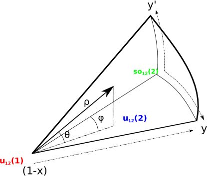
Figure 1: (Color online) Representation of the two-Lipkin model parameter space. For completeness, the symmetries of the model are also indicated in the diagram.

IV Numerical analysis of the phase diagram

In order to study the structure of the two-fluid Lipkin model phase diagram as a function of the control parameters, ($x,y_{1},y_{2}$), we have found appropriate to introduce alternative control parameters, ($y,y^{\prime}$), defined by,

$$y=\frac{y_{1}+y_{2}}{2},\qquad y^{\prime}=\frac{y_{1}-y_{2}}{2}.$$ (29)

With this change, we can study the phase diagram in terms of the coordinates,

$$\rho=1-x;\qquad\theta=\frac{\pi}{24}(y_{1}-y_{2})=\frac{\pi}{12}y^{\prime};\qquad\phi=\frac{\pi}{24}(y_{1}+y_{2})=\frac{\pi}{12}y.$$ (30)

Where we have assumed a maximum value for $|y_{1}|$ and $|y_{2}|$ equal to 2 so as the angles $\theta$ and $\phi$ are defined between $-\pi/6$ and $\pi/6$ (see Fig. 1).

The geometric representation of the two-fluid consistent-Q-like Lipkin Hamiltonian will be, therefore, a pyramid in this phase space. One vertex corresponds to the $u_{12}(1)$ limit of the model ($x=1$). The bottom plane, $y_{1}=y_{2}\Rightarrow$ $y^{\prime}=0$, corresponds to the $u_{12}(2)$ dynamical algebra (both fluid are combined symmetrically into a single $u(2)$) algebra, which is equivalent at the mean-field level to the single Lipkin model (in the IBM-2 case, the equivalent horizontal plane represents the IBM-1, i.e., a symmetric combination of the two boson fluids). In this plane, the line $y_{1}=y_{2}=0$ ($y=y^{\prime}=0$) goes from the $so_{12}(2)$ to the $u_{12}(1)$ limit. As soon as one considers $y_{1}\neq y_{2}$ ($y^{\prime}\neq 0$) one moves in the vertical direction of the pyramid and any present symmetry will become broken. Of special interest is the vertical plane $y_{1}=-y_{2}$ ($y=0,y^{\prime}\neq 0$) because, for this combination of parameters, the mean-field energy is invariant under the transformation $\beta_{1}\rightarrow-\beta_{2}$. Note that the two remaining vertexes do not correspond to any symmetry of the model (in the case of IBM-2 they correspond to the $su(3)$ and $su(3)^{*}$ symmetries).

As a first step to establish the phase diagram of the model, in the following of this section we will present numerical studies of different trajectories within the phase space of the model ($\rho,y,y^{\prime}$) in order to identify the different phases and phase transition surfaces/lines.

To get a geometrical idea about system shapes in the different regions of the phase space, we note that the region around the $u_{12}(1)$ vertex corresponds to values of the variational parameters $\beta_{1}$ and $\beta_{2}$ equal to zero. Since $\beta$ parameters give the weight of the $t$ bosons in the boson condensate, $\beta=0$ implies a condensate of spherical $s$ bosons. Consequently the phase around the $u_{12}(1)$ vertex is called symmetric or spherical. The corresponding spectrum will become nearly harmonic. When the system goes well apart of the $u_{12}(1)$ vertex, both variational parameters, $\beta_{1}$ and $\beta_{2}$ become different from zero. This makes that the boson condensate in both fluids has a fraction of $t$ bosons. Thus, this phase is called non-symmetric or deformed. The horizontal plane corresponds to $\beta_{1}=\beta_{2}$ which implies equal deformations for both fluids what bring us back to the single Lipkin model.

To study the possible phase transitions that occur in the phase diagram we have performed numerical analysis through selected straight trajectories in the phase space. For each of them the equilibrium energy, the derivatives of the energy functional, and also the equilibrium values of the variational parameters have been analyzed. All exact calculations presented in this section correspond to $N_{1}=N_{2}=500$ but similar studies can be done for $N_{1}\neq N_{2}$ and other boson numbers.

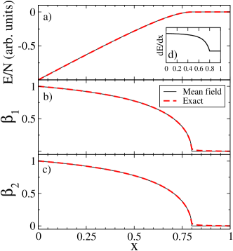
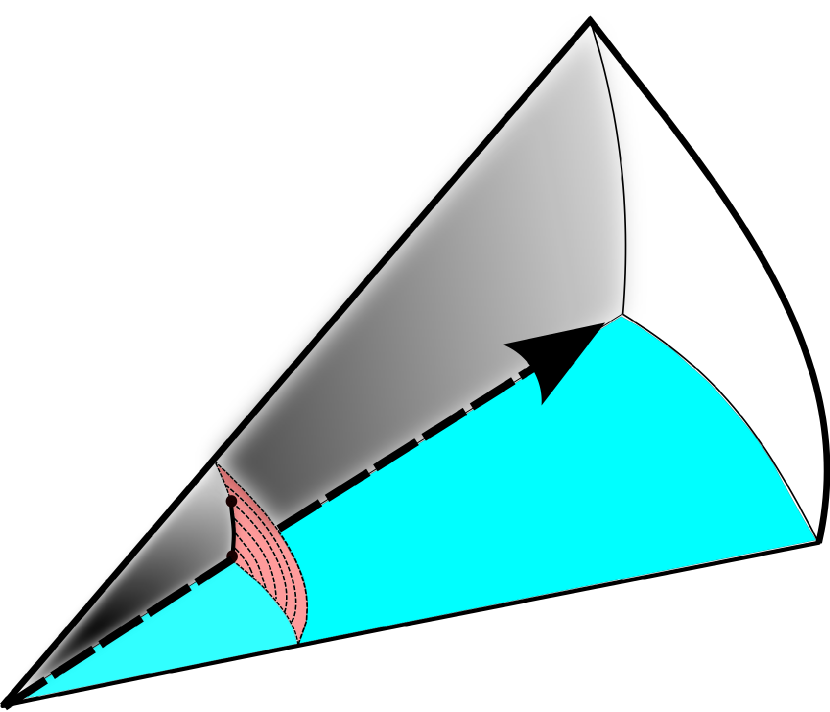
e)

Figure 2: (Color online) Transition line for $y=0$ and $y^{\prime}=0$ changing the control parameter $x$. In the different panels we plot as a function of $x$: panel (a) the energy per boson (in arbitrary units), panel (b) the order parameter $\beta_{1}$ (dimensionless), panel (c) the order parameter $\beta_{2}$ (dimensionless), panel (d) $dE/dx$ in arbitrary units, and panel (e) representation of the trajectory in the control parameter space. Full thin black lines correspond to the mean-field results while dashed thick red lines are the exact calculation with $N_{1}=N_{2}=500$.

IV.1 Plane $y^{\prime}=0$

First, we start analyzing the bottom plane that corresponds to $y_{1}=y_{2}=y$ and $y^{\prime}=0$, therefore an energy surface fully equivalent to the single Linkin case is reproduced. In Fig. 2 the line $y_{1}=y_{2}=y=0$ and $y^{\prime}=0$ is studied (see panel e), in the figure the energy per particle (panel a), as well as, the deformation parameters (panels b and c) as a function of the control parameter $x$ are plotted. We have also included the function $dE/dx$ in panel (d). One can clearly see how a phase transition setups around $x=4/5$. At the mean field level the phase transition is established as second order since a discontinuity appears in the second derivative of the energy (see panel (d) where $dE/dx$ is continuous but not its derivative) and in the first derivative of the order parameters. Note that due to symmetry arguments $\beta_{1}=\beta_{2}$ over the whole plane. In Fig. 2 the mean-field results (black full line) are shown together with the exact result coming from direct diagonalization (red dashed line) for $N_{1}=N_{2}=500$. In the exact calculation, the values of the order parameters are extracted using this relationship,

$$\beta_{i}=\sqrt{\frac{\langle n_{t_{i}}\rangle}{N_{i}-\langle n_{t_{i}}\rangle}}.$$ (31)

Excellent agreement is found between mean-field and exact results since the number of bosons considered in the exact diagonalization is large enough.

In Fig. 3 we repeat the same calculation but for the line $y_{1}=y_{2}=y=1$ and $y^{\prime}=0$ (see panel e). In this case, a first order phase transition is observed for $x_{c}=5/6=0.833$. The order of the phase transition is clear from the discontinuity in the value of the order parameter at the mentioned phase transition point, as well as for the discontinuity in $dE/dx$ (see panel (d)). In general, for $y_{1}=y_{2}=y\neq 0$ the phase transition is of first order and the critical point is located at Vida06

$$x_{c}=\frac{4+y^{2}}{5+y^{2}}.$$ (32)

Consequently, the location of the critical point is shifted to slightly larger values of $x$ as $y$ increases, while the jump of the order parameter at the phase transition point becomes larger.

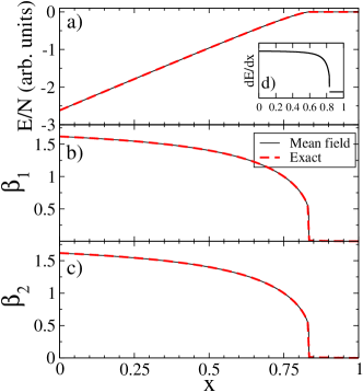
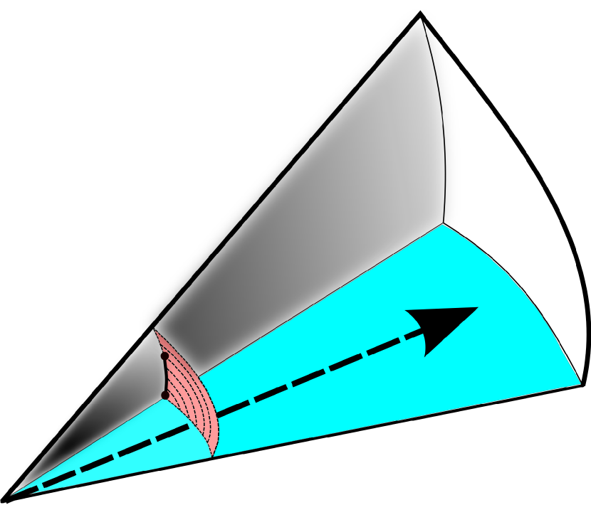
e)

Figure 3: (Color online) Same as Fig. 2 but with $y_{1}=y_{2}=y=1$ and $y^{\prime}=0$.

IV.2 Volume region inside the pyramid: $y\neq 0$ and $y^{\prime}\neq 0$

Now a trajectory going through the inner part of the pyramid is analyzed. In particular, the case $y_{1}=1$ and $y_{2}=-1/2$, i.e., $y=1/4$ and $y^{\prime}=3/4$, is presented in Fig. 4 (panel e). From this figure, it is clear that a first order phase transition is observed at around $x_{c}=0.0.805$. Several trajectories inside the pyramid have been studied with similar results (the dependence on $y$ and $y^{\prime}$ of $x_{c}$ is involved and cannot be obtained in a closed form). The size of the discontinuity depends on how far the values of $y$ and $y^{\prime}$ are from $y=0$ and $y^{\prime}=0$.

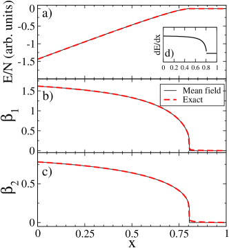
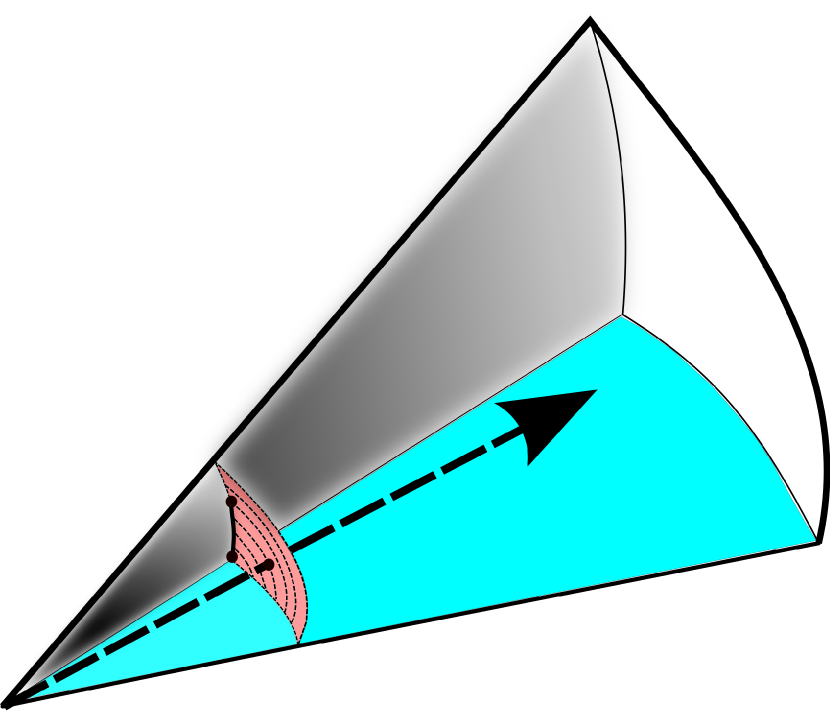
e)

Figure 4: (Color online) Same as Fig. 2 but with $y_{1}=1$ and $y_{2}=-1/2$ ($y=1/4$ and $y^{\prime}=3/4$).

IV.3 The vertical plane: $y=0$

The vertical plane corresponds to $y_{1}=-y_{2}$, what means $y=0$ and $y^{\prime}=y_{1}=-y_{2}$ and, as we are showing below, is the most interesting case. Several trajectories inside this plane will be presented and one crossing the plane from positive to negative $\beta$-values.

The first trajectory is the line $y_{1}=-y_{2}=y^{\prime}=1/2$ (panel e) and the results are depicted in Fig. 5. A second order phase transition at $x_{c}=0.8$ is observed. The order parameters, coming from the exact diagonalization, show an oscillatory pattern due to the degeneracy of two states that are related with the two minima present in the $\beta_{1}-\beta_{2}$ plane of the mean-field energy (see Fig. 9). The degeneracy of two states with different deformation makes that the order parameter obtained from the diagonalization may jump from one minimum to the other (between the two degenerate mean-field values). Indeed, for a given value of $x$ the equilibrium value of one of the order parameters will correspond to $\beta_{1}=\beta_{x}$ and $\beta_{2}=\beta^{\prime}_{x}$, while the other to $\beta_{1}=-\beta^{\prime}_{x}$ and $\beta_{2}=-\beta_{x}$. Note that we have taken the absolute value of $|\beta_{i}|$ for a better comparison with the exact results, which are, by definition, positive.

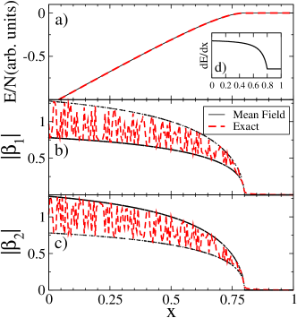
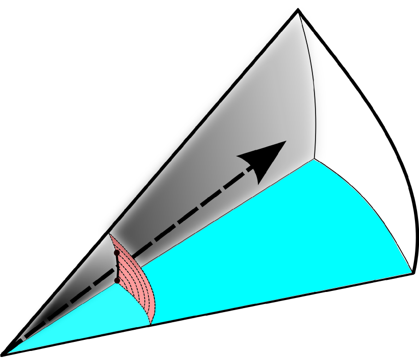
e)

Figure 5: (Color online) Same as Fig. 2 but with $y_{1}=-y_{2}=y^{\prime}=1/2$ and $y=0$.

In Fig. 6 a calculation along the line $y_{1}=-y_{2}=y^{\prime}=1$ and $y=0$ is presented. In this case is difficult to disentangle the order of the phase transition just looking at the energy and the order parameters, however, in the inset panel it is clear that a discontinuity in the second derivative of the energy exists, which, once more, happens at around $x_{c}=0.8$. In Section V.2 we will see in detail that, indeed, a divergence in $d^{2}E/dx^{2}$ exists and we will try to understand the reason why there is a divergence in the second derivative. Note that $dE/dx$ becomes vertical at $x=4/5$ from the left side.

Finally, in Fig. 7 the calculation along the line $y_{1}=-y_{2}=y^{\prime}=3/2$ and $y=0$ is shown. In this calculation, it is easily appreciated the onset of a first order phase transition at around $x_{c}=0.81$, i.e., discontinuity in the first derivative of the energy and in the value of the order parameters.

After the analysis of the different paths in the plane $y=0$, corresponding to different $y^{\prime}$ values, one is tempted to conclude that there is a line of phase transition for values of $x$ around $x_{c}=0.8$. However, the value $y^{\prime}=1$ separates this line into two parts: for values $y^{\prime}\leq 1$ the line corresponds to a second order phase transition, while for values $y^{\prime}>1$ the line is of first order. This weak conclusion, based on numerical calculations, will be confirmed in Section V.2 through an analytic study.

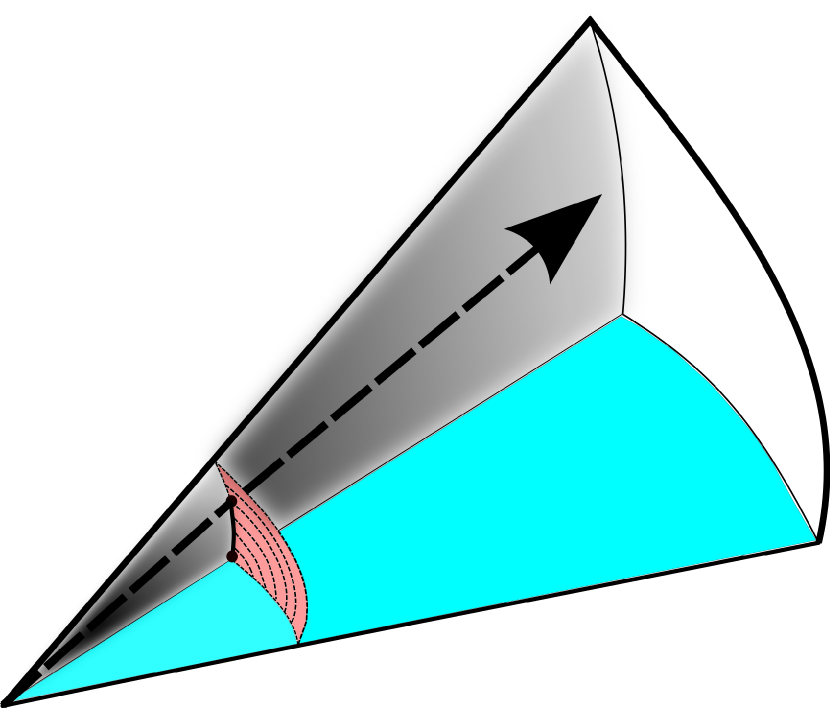
e)

Figure 6: (Color online) Same as Fig. 2 but with $y_{1}=-y_{2}=y^{\prime}=1$ and $y=0$.

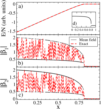
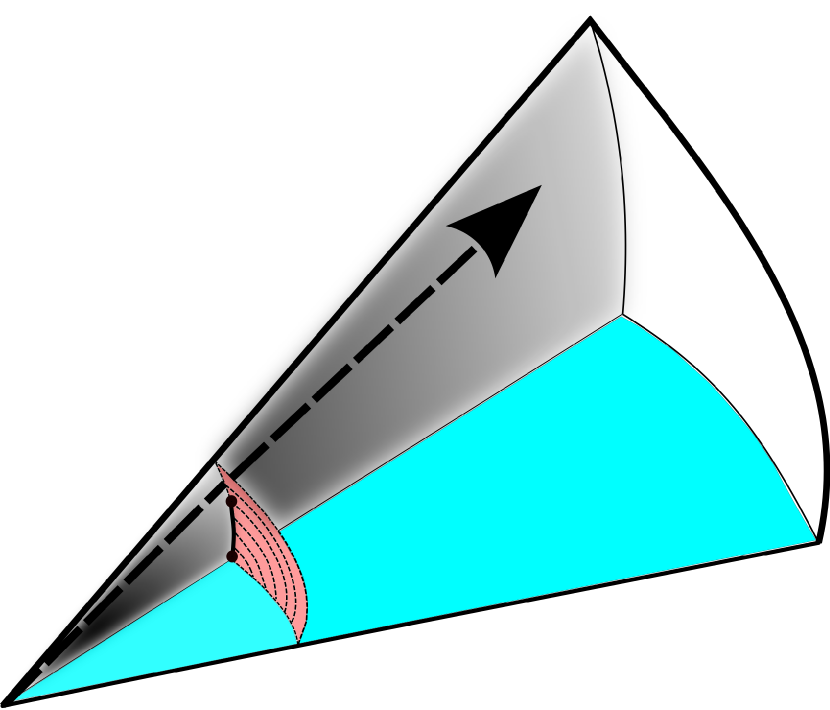
e)

Figure 7: (Color online) Same as Fig. 2 but with $y_{1}=-y_{2}=y^{\prime}=3/2$ and $y=0$.

It is worth noting that the vertical plane $y=0$, for $x<4/5$ separates two deformed regions. In order to study the transition between both deformed regions, finally, a line crossing this vertical surface is analyzed. Here, because of the presence of two degenerated minima a first order phase transition for the whole vertical surface in the deformed phase is expected. This is fully confirmed in Fig. 8 (parameters $x=0.5$, $y=1$), where the first order phase transition appears for $y_{2}=-1$. Please, note that in Fig. 8 we have changed by hand the value of $\beta$ coming from the exact calculation (it is, by definition, always positive) for a better comparison with the mean-field results.

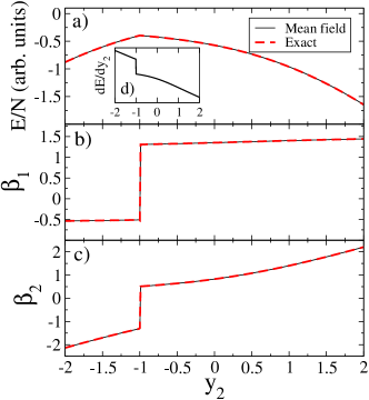
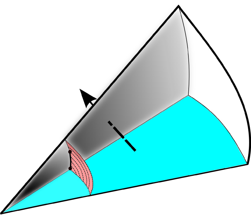
e)

Figure 8: (Color online) Transition for $x=0$ and $y_{1}=1$ as a function of $y_{2}$. In panel (a) the energy per boson is plotted in arbitrary units, in panel (b) the order parameter $\beta_{1}$ (dimensionless) is shown, in panel (c) the order parameter $\beta_{2}$ (dimensionless) is represented, in panel (d) $dE/dx$ in arbitrary units is plotted, and in panel (e) the representation of the trajectory in the control parameter space is shown. Full thin black lines correspond to the mean-field results while dashed thick red lines are the exact calculation with $N_{1}=N_{2}=500$.

Combining all the preceding evidences one gets the phase diagram depicted in Fig. 9, where one can appreciate a first order phase transition surface separating the symmetric (spherical) and non-symmetric (deformed) phases and the first order phase transition vertical surface separating two different deformed phases. We will see in next section that the intersection line between both surfaces, from $y^{\prime}=0$ up to $y^{\prime}=1$ is a second order phase transition line, while for larger values of $y^{\prime}$ it becomes first order. Note that the phase diagram can be extended to negative values of $y$ and $y^{\prime}$, with the first order phase transition surface separating spherical and deformed phase extended to four quadrants and the vertical first order phase transition surface and the second order phase transition line extended to negative values of $y^{\prime}$.

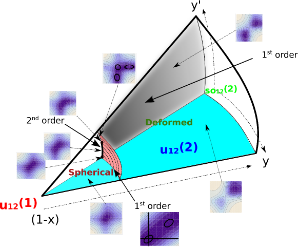
Figure 9: (Color online) Phase diagram of the consistent-Q like two-fluid Lipkin model. In the diagram the different phases are represented: spherical and deformed, the first order QPT surfaces and the second order QPT line. Moreover, the relevant control parameters and dynamical symmetries also are shown.

V Local Taylor expansion and catastrophe theory

V.1 Fundamentals

Once the main structure of the phase diagram of the model is known numerically, it is necessary to perform an analytic study to determine unambiguously the order of the phase transitions of surfaces and lines appearing in the phase diagram and to understand why the QPT areas are precisely located there. To carry out this task we will make use of catastrophe theory (CT) Thom75 , which is an ideal tool for such an end.

In general, the aim of CT is to study a given potential, $V(\vec{x},\vec{\lambda})\in\Re$ (in our case the mean-field energy surface of the model) or a family of potentials that are function of a set of order parameters, $\vec{x}\in\Re^{n}$ and that depend on a set of control parameters, $\vec{\lambda}\in\Re^{r}$, and to study the qualitative behavior of the potential, e.g., number of minima and maxima, as a function of the control parameters. To proceed one should start looking for the stationary points (also known as critical points), i.e., those whose gradient vanish and classify them according to their stability: i) points where the determinant of the Hessian matrix is different from zero, called isolated, non-degenerated or Morse points, and ii) points where the determinant of the Hessian matrix is zero, called non-isolated, degenerated or non-Morse points. In summary, points of a family of smooth potentials can be classified according to their gradient and Hessian matrix ${\cal H}$ as:

• Regular points: $\nabla V\neq 0$.

• Morse points (isolated critical points): $\nabla V=0$ and $|{\cal H}|\neq 0$.

• Non-Morse points (degenerated critical points): $\nabla V=0$ and $|{\cal H}|=0$.

Morse theorem Post78 ; Gilm81 guarantees that around a Morse point, a smooth potential is equivalent to a quadratic form, performing a smooth non-linear change of variables. Therefore, the potential is stable under small perturbations around Morse points. At non-Morse points the potential cannot be written as a quadratic form because the Hessian matrix has at least one zero eigenvalue. Around non-Morse points CT will provide useful information on how the qualitative shape of the potential will evolve under small variations of the order parameters.

In the case of several order parameters, Thom’s splitting lemma Thom75 guarantees that a smooth potential at non-Morse points can be written as a sum of a quadratic form, associated to the subspace with nonzero eigenvalues, plus a function containing the variables associated to the zero eigenvalues of the Hessian matrix.

The first step in the CT program is to find out the critical points of the energy surface ($\nabla E=0$). Among them, the most important is the most degenerate one, i.e., the point where most successive derivatives vanish. This point is the fundamental root taking place at definite values of the control parameters which we will call critical values. We next proceed making use of a Taylor expansion of the energy surface around the fundamental root. A Taylor expansion around such a point is also valid for the critical points that arise from the fundamental root when the degeneracy is broken. Depending on the degeneracy of the fundamental root the number of extremes that can be analyzed simultaneously will change. It is worth to note that the different minima related with the appearance of a critical phenomenon arise from a degenerated non-Morse point.

When the potential depends on several variables, as the case for the two-fluid Lipkin model is, it is important to separate the variables into two sets, depending on how Hessian eigenvalues behave. On one hand, one has the variables associated to the subspace with vanishing Hessian eigenvalues, called bad or essential variables, while, on the other hand, there is a set of variables related to the non-vanishing Hessian eigenvalues, called good or non-essential variables. Therefore, as a consequence of the splitting lemma Thom75 , the potential could be separated into a part depending on the essential variables and into another part depending on the non-essential ones by rewriting it in terms of the eigenvectors of the Hessian matrix Gilm81 . The appearance of critical phenomena will be associated exclusively with the behavior of the essential variables, i.e., the variables that can be identified as order parameters of the system.

V.2 Application to the two-fluid Lipkin model

According to Eqs. (27) and (28) the most degenerated critical point for the two-fluid Lipkin model (15) corresponds to $\beta_{1}=0$ and $\beta_{2}=0$ (all derivatives up to fourth order vanish for an appropriated set of parameters) and, taking into account the shape of the phase diagram, all the critical points that can eventually arise in the energy surface are born from this most degenerated critical point. Since there are two shape variables it is necessary to construct, first, the Hessian matrix associated to the energy surface (27),

$$\cal{H}=\left(\begin{array}[]{cc}\partial^{2}E/\partial\beta_{1}^{2}&\partial^{2}E/\partial\beta_{1}\partial\beta_{2}\\ \partial^{2}E/\partial\beta_{2}\partial\beta_{1}&\partial^{2}E/\partial\beta_{2}^{2}\end{array}\right)=\left(\begin{array}[]{cc}3x-2&2x-2\\ 2x-2&3x-2\end{array}\right).$$ (33)

The two eigenvalues are $5x-4$ and $x$, and the corresponding eigenvectors are,

$$\beta_{a} = \frac{1}{2}~{}(\beta_{1}+\beta_{2}),$$ (34)

$$\beta_{b} = \frac{1}{2}~{}(\beta_{1}-\beta_{2}).$$ (35)

The eigenvalue associated to $\beta_{a}$ vanishes for $x=4/5$ while the one associated to $\beta_{b}$ only vanishes for the trivial case $x=0$. Therefore, the essential variable turns out to be $\beta_{a}$, while $\beta_{b}$ becomes the non-essential one, i.e., the origin in this variable behaves as a Morse point.

Next step is to carry out a Taylor expansion in $\beta_{a}$ and $\beta_{b}$ around zero. Because we use $\beta_{a}$ and $\beta_{b}$, the quadratic term $\beta_{a}\beta_{b}$ will not be present in the Taylor expansion. Note that we are considering the case $N_{1}=N_{2}$.

$$\frac{E(x,y,y^{\prime},\beta_{a},\beta_{b})}{N} = (5x-4)\beta_{a}^{2}+4(x-1)y\beta_{a}^{3}+\left(8-9x+y^{2}(x-1)\right)\beta_{a}^{4}+\Theta(\beta_{a}^{5})+x\beta_{b}^{2}+\Theta(\beta_{a}\beta_{b}^{2},\beta_{b}\beta_{a}^{2}).$$

In order to cancel the higher order terms ($\beta_{a}^{i}\beta_{b}^{j}$ with $j>1$) we have to implement a nonlinear transformation in $\beta_{b}$

$$\tilde{\beta_{b}}=\beta_{b}+\sum_{i+j>1}a_{ij}\beta_{a}^{i}\beta_{b}^{j}.$$ (36)

After imposing the cancellation of the crossing terms and determining the value of $a_{ij}$, we get the next expression that is valid in the neighborhood of $\beta_{a}=0$, but for any value of $\beta_{b}$ (note that in order to simplify the notation we continue referring to the non-essential variable as $\beta_{b}$ instead of $\tilde{\beta_{b}}$),

$$\frac{E(x,y,y^{\prime},\beta_{a},\beta_{b})}{N} = (5x-4)\beta_{a}^{2}+4(x-1)y\beta_{a}^{3}+\left(8-9x+y^{2}(x-1)-\frac{16{y^{\prime}}^{2}}{x}(x-1)^{2}\right)\beta_{a}^{4}$$ (37)

$$+ \frac{8(x-1)y\left((6{y^{\prime}}^{2}-1)x^{2}-14{y^{\prime}}^{2}x+8{y^{\prime}}^{2}\right)}{x^{2}}\beta_{a}^{5}$$

$$+ \frac{1}{x^{3}}\left((64{y^{\prime}}^{4}-384{y^{\prime}}^{2}-2y^{2}(82{y^{\prime}}^{2}+1)+13)x^{4}+2(-96{y^{\prime}}^{4}+576{y^{\prime}}^{2}\right.$$

$$+ y^{2}(372{y^{\prime}}^{2}+1)-6)x^{3}+4{y^{\prime}}^{2}(48({y^{\prime}}^{2}-6)-313y^{2})x^{2}$$

$$+ \left.32{y^{\prime}}^{2}(29y^{2}-2{y^{\prime}}^{2}+12)x-256y^{2}{y^{\prime}}^{2}\right)\beta_{a}^{6}$$

$$+ O(\beta_{a}^{7})+x\beta_{b}^{2}.$$

The number of lower order terms that are kept in the Taylor expansion without loosing substantial information with respect to the original function (problem of determinacy) is determined studying the terms in the Taylor expansion that can be canceled out with appropriated particular values of the control parameters. For Eq. (37) the values of the control parameters, $x=4/5$, $y=0$ and $y^{\prime}=1$ cancel all terms up to $\beta_{a}^{5}$. Therefore, the dominant remaining term is $\beta_{a}^{6}$ and it is said that the function is $6-determined$. Hence, the number of essential parameters will be $3$. Consequently, the relevant elementary catastrophe of this model is the butterfly (A₊₅) Gilm81 . It is worth mentioning that the butterfly has a codimension equal to $4$, i.e., the number of essential parameters is $4$. In our case, due to the function symmetry, the number of parameters is only $3$. In general, depending on the values selected for the control parameters, the potential energy may have three, two, or one local minima. Please note that Eq. (37) does not correspond to the canonical form of the butterfly because it presents a fifth order term instead of the first order one. However, one always can perform a shift transformation in the $\beta_{a}$ variable to recover the canonical form.

In order to determine the order of the phase transitions, already studied numerically in the preceding section, we can take advantage of Eq. (37). In general, for any situation with $y\neq 0$ the cubic (and fifth) term always survives for any value of $y^{\prime}$ and, therefore, the phase transition will become first order. The reason is simple, the presence of a cubic (and fifth) term guaranties the possible appearance of several critical points (i.e., a region of coexistence), three critical points (two minima and one maximum) when the $\beta_{a}^{2}$ coefficient and the $\beta_{a}^{4}$ coefficient are positive and five critical points (three minima and two maxima) when the $\beta_{a}^{2}$ coefficient is positive and the $\beta_{a}^{4}$ coefficient is negative (see below for more details). Note that in our case, the $\beta_{a}^{6}$ coefficient is always positive. Indeed, this particular situation is precisely the one necessary to develop a first order phase transition. This happens in almost the whole surface separating the symmetric (spherical) and non-symmetric (deformed) phases.

To know the character of the vertical surface, $y=0$ (with $x<4/5$), one can note that the lowest leading terms are: $\beta_{a}^{2}$ with negative coefficient and $\beta_{a}^{4}$ with positive coefficient. This potential gives rise to two degenerated minima symmetric with respect to the origin, $\beta_{a}=0$. As soon as one perturbs the system, changing $y$ (to either positive or negative values) the degeneracy is broken and one of the deformed minima is lower in energy. Therefore, this situation corresponds to a first order phase transition since the order parameter will jump suddenly from one to the other minimum.

It is also of interest to see how one can recover the case corresponding to the single Lipkin, i.e., $y^{\prime}=0$. For this case (horizontal plane) the energy surface reads as,

$$\frac{E(x,y,y^{\prime},\beta_{a},\beta_{b})}{N} = (5x-4)\beta_{a}^{2}+4(x-1)y\beta_{a}^{3}+\left(y^{2}(x-1)+8-9x\right)\beta_{a}^{4}+O(\beta_{a}^{5})+x\beta_{b}^{2},$$ (38)

where one can easily single out that for the line $x=4/5$, values $y\neq 0$ produce a first order phase transition since the cubic term is present. For the particular value $y=0$ the cubic term vanishes and, therefore, the transition is no longer of first order, but of second order.

Finally, a most interesting case is the intersection line between the surfaces $y=0$ (vertical plane, separating two regions of different deformation) and $x\approx 4/5$ (spherical surface separating spherical from deformed shapes). For this situation, the energy functional is written as,

$$\frac{E(x,y^{\prime},\beta_{a},\beta_{b})}{N} = (5x-4)\beta_{a}^{2}+\left(8-9x-\frac{16(x-1)^{2}y^{\prime 2}}{x}\right)\beta_{a}^{4}$$ (39)

$$+ \frac{1}{2}\left(26x-24+\frac{128(x-1)^{3}y^{\prime 2}(y^{\prime 2}-6)}{x^{2}}\right)\beta_{a}^{6}+O(\beta_{a}^{7})+x\beta_{b}^{2}.$$

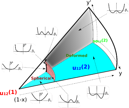
Figure 10: (Color online) Same as Fig. 9 but including the corresponding energy curves as a function of the essential order parameter $\beta_{a}$.

This situation looks like the case $y=y^{\prime}=0$, because no odd terms appear in the expansion and only the onset of a second order phase transition is expected. However, there are fundamental differences. The key point to disentangle the stability structure of the energy surface is the sign of the fourth order coefficient. The phase transition at $x=4/5$ is indeed of second order if the fourth order coefficient remains positive but will change to first order otherwise. There is a critical value for $y^{\prime}$ for which the fourth order coefficient vanishes, i.e., $y^{\prime}=1$ and $x=4/5$. At this point, the only term that survives in the energy functional is the sixth order term. The most important consequence is that at this point the energy surface is very flat (as $\beta_{a}^{6}$). Going to values with $y^{\prime}>1$, the fourth order coefficient changes to negative sign, which implies that there is no longer a second order phase transition, but a first order one since, in this case, there is a sudden change in the order parameter when crossing the QPT point. To understand this fact let us write in a more compact form the Taylor expansion (39) as,

$$E=\frac{A}{2}\beta^{2}+\frac{B}{4}\beta^{4}+\frac{C}{6}\beta^{6},$$ (40)

where $C>0$. According to Eq. (39): $A>0$ for $x>4/5$, $A<0$ for $x<4/5$ and $A=0$ for $x=4/5$; at $x=4/5$, $B>0$ for $y^{\prime}<1$, $B<0$ for $y^{\prime}>1$, and $B=0$ for $y^{\prime}=1$; for $x\approx 4/5$ $C$ is always positive. Equation $dE/d\beta=0$ has as solutions,

$$\beta = 0,$$

$$\beta^{2} = \frac{-B\pm\sqrt{B^{2}-4AC}}{2C}.$$ (41)

The spherical solution ($\beta=0$) corresponds to a minimum if $A>0$, i.e., $x>4/5$ (to a maximum if $A<0$, i.e., $x<4/5$ ), irrespective of the $B$ sign, i.e., independently of the $y^{\prime}$ value. For $A<0$ and $B>0$ (which occurs for $|y^{\prime}|<1$) two deformed critical points exist (symmetric with respect to the origin), which correspond to minima since, as discussed above, $\beta=0$ corresponds, in this case, to a maximum. Note that for $A=0$ the two deformed minima merge into a flat spherical one, never coexisting several minima. Therefore, the line $y=0$ and $A=0$ corresponds to a second order phase transition while $|y^{\prime}|<1$.

For $A\gtrsim 0$ and $B<0$ (which occurs for $y^{\prime}>1$ and $x\gtrsim 4/5$) five critical points coexist for $B^{2}>4AC$, one corresponds to the spherical minimum, and other two correspond to two deformed minima (symmetric with respect to the origin, $\beta_{a}=0$). The other two extremes correspond to maxima (symmetric with respect to the origin). The particular region $y=0$, $A=0$ ($x=4/5$) for values $y^{\prime}>1$, is a region of coexistence of three minima, one spherical and two deformed. At the critical point all three minima are degenerated. As a consequence, a first order phase transition develops around this line. The first order phase transition line is defined then by

$$A=\frac{B^{2}}{4C},$$ (42)

and is bounded by the spinodal ($(\partial^{2}E/\partial\beta^{2})_{\beta=0}=0$) and the antispinodal ($(\partial^{2}E/\partial\beta^{2})_{\beta=\beta_{c}\neq 0}=0$) lines given by,

$$A = 0~{}~{}~{}~{}~{}~{}~{}~{}~{}~{}~{}~{}~{}~{}\textrm{(spinodal)},$$ (43)

$$A = \frac{3B^{2}}{16C}~{}~{}~{}~{}\textrm{(antispinodal)}.$$ (44)

For the case $B^{2}<4AC$ only the spherical minimum exists.

It is worth analyzing what happens at the special line $y=0$ and $y^{\prime}=1$. For this line $B=0$ and the energy surface presents three critical points when $A<0$ ($x<4/5$),

$$\beta = 0,$$ (45)

$$\beta = \pm(\frac{-A}{C})^{1/4}.$$ (46)

The first one, spherical, corresponds to a maximum and the second and the third, deformed and symmetric with respect to the origin, correspond to minima. For $A>0$ ($x>4/5$) only the minimum at $\beta=0$ survives. In order to study the QPT at $x=4/5$, one can write the energy at the equilibrium $\beta-$value (46) that is,

$$E = \frac{(-A)^{3/2}}{3\sqrt{C}}~{}~{}~{}~{}~{}~{}~{}~{}~{}~{}~{}~{}~{}~{}~{}~{}~{}~{}\textrm{for}~{}~{}A<0,$$ (47)

$$E = 0~{}~{}~{}~{}~{}~{}~{}~{}~{}~{}~{}~{}~{}~{}~{}~{}~{}~{}~{}~{}~{}~{}~{}~{}~{}~{}~{}~{}~{}\textrm{for}~{}~{}A>0.$$ (48)

Its first derivative with respect to $A$ is

$$\frac{dE}{dA} = \frac{-\sqrt{-A}}{2\sqrt{C}}~{}~{}~{}~{}~{}~{}~{}~{}~{}~{}~{}~{}~{}~{}~{}\textrm{for}~{}~{}A<0,$$ (49)

$$\frac{dE}{dA} = 0~{}~{}~{}~{}~{}~{}~{}~{}~{}~{}~{}~{}~{}~{}~{}~{}~{}~{}~{}~{}~{}~{}~{}~{}~{}\textrm{for}~{}~{}A>0.$$ (50)

Therefore, the transition is not of first order. Performing the second order derivative,

$$\frac{d^{2}E}{dA^{2}} = \frac{-1}{4\sqrt{-AC}},~{}~{}~{}~{}~{}~{}~{}~{}~{}~{}~{}~{}~{}~{}~{}~{}~{}~{}~{}\textrm{for}~{}~{}A<0,$$ (51)

$$\frac{d^{2}E}{dA^{2}} = 0~{}~{}~{}~{}~{}~{}~{}~{}~{}~{}~{}~{}~{}~{}~{}~{}~{}~{}~{}~{}~{}~{}~{}~{}~{}~{}~{}~{}~{}~{}~{}\textrm{for}~{}~{}A>0.$$ (52)

Therefore, a discontinuity appears in the second derivative with respect to the control parameter. Indeed in the deformed side the second derivative diverges to $-\infty$.

In Fig. 10 we show, once more, the phase diagram, but in this case plotting the corresponding energy curves as a function of the value of the essential variable. In this figure one can appreciate in a cleaner way how the first order vertical plane is related to two symmetric degenerated minima, symmetric with respect to $\beta_{a}=0$, while the first order surface separating spherical and deformed phases corresponds also to two degenerated minima, spherical and deformed. The line $x=4/5$, $y=0$, $y^{\prime}<1$ corresponds to a $\beta_{1}^{4}$ energy curve, i.e., to a cusp line. The point $x=4/5$, $y=0$, $y^{\prime}=1$ corresponds to a $\beta_{1}^{6}$ energy curve and, finally, a first order phase transition line appears for $x\approx 4/5$, $y=0$, $y^{\prime}>1$ with three degenerated minima. The behavior of this first order phase transition area is explained in detail in Fig. 11, where as a function of the control parameters $A$ and $B$ is depicted the phase diagram, separating the areas corresponding to spherical (blue area), deformed shapes (red area) or coexistence area (yellow area). Also spinodal, antispinodal and first order line are shown.

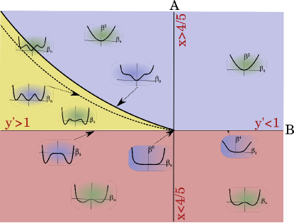
Figure 11: (Color online) Representation of the butterfly catastrophe (without odd-power terms), Eq. (40), as a function of the control parameters $A$ and $B$. The energy curves that characterize every region are depicted, besides, the curves corresponding to lines/points with degenerated critical points are also depicted.

At the point $A=0$, $B=0$, i.e., $x=4/5$, $y=0$, and $y^{\prime}=1$ the second order phase transition line ($B>0$) and the spinodal, antispinodal and first order phase transition merge. This point is known as tricritical point while the first order phase transition line corresponds to a triple point curve where three minima are degenerated and coexist.

The inclusion of a third (and a fifth) order term in the potential (40) will break the symmetry of the function. The consequence will be the appearance of a coexistence region for the cusp line and, therefore its transformation in a first order phase transition line. In the case of the coexistence area with $B<0$ the asymmetry generated in the energy curves will make impossible the degeneracy of three minima, but however, will continue being possible the degeneracy of the spherical and one of the deformed minima. Moreover the spinodal line is still at $A=0$ too, though the antispinodal one will be shifted. As a consecuence, in this case, the phase transition is still of first order.

VI Summary and conclusions

In this work the mean-field energy surface of the consistent-Q like double Lipkin Hamiltonian has been studied. The analyzed Hamiltonian resembles the IBM-2 Hamiltonian of interest in Nuclear Physics. The phase diagram of the model has been established both numerical and analytically. The mean-field numerical calculations have been compared with direct diagonalizations and good agreement has been reached. The analytical study has been performed using the catastrophe theory and it has been found that the energy can be successfully described by the butterfly catastrophe.

Therefore, the phase diagram of the model has been obtained, including phases, locations of the QPT phase transitions and their orders. In particular, there are three phases: spherical and two different deformed ones. The surface separating spherical and both deformed phases is of first order: two minima, one spherical and one deformed, which are degenerated at the phase transition point. Moreover, the vertical plane separating both deformed phases is also of first order: two deformed minima with different deformations are degenerated and separated by a maximum at $\beta_{a}=0$. These two surfaces intersect in the line ($x=4/5$, $y=0$), this is of second order for $0<y^{\prime}\leq 1$ and transforms to a first order phase transition for $y^{\prime}>1$. The part of the line ($x=4/5$, $y=0$, $0<y^{\prime}<1$) corresponds to a flat surface (goes as $\beta_{a}^{4}$). At the point ($x=4/5$, $y=0$, $y^{\prime}=1$) the energy surface is even flatter, goes as $\beta_{a}^{6}$. Finally, in the part of the line ($x\approx 4/5$, $y=0$, $y^{\prime}>1$) three degenerated minima coexist (one spherical and two deformed ones). The point $x=4/5$, $y=0$ and $y^{\prime}=0$ corresponds to a tricritical point in the language of the Ginzburg-Landau theory for phase transitions.

VII Acknowledgment

This work has been supported by the Spanish Ministerio de Economía y Competitividad and the European regional development fund (FEDER) under Project No. FIS2011-28738-C02-01, FIS2011-28738-C02-02, FIS2014-53448-C2-1-P, FIS2014-53448-C2-2-P, and by Spanish Consolider-Ingenio 2010 (CPANCSD2007-00042).

References

- (1) R.F. Casten and E.A. McCutchan, J. Phys. G 34, R285 (2007).
- (2) P. Cejnar and J. Jolie, Prog. Part. Nucl. Phys. 62, 210 (2009).
- (3) P. Cejnar, J. Jolie, and R.F. Casten, Rev. Mod. Phys. 82, 2155 (2010).
- (4) F. Iachello and F. Pérez-Bernal, Mol. Phys. 106, 223 (2008).
- (5) P. Pérez-Fernández, J.M. Arias, J.E. García-Ramos, and F. Pérez-Bernal, Phys. Rev. A 83, 062125 (2011).
- (6) C. Emary and T. Brandes, Phys. Rev. Lett. 90, 044101 (2003); Phys. Rev. E 67, 066203 (2003); N. Lambert, C. Emary, and T. Brandes, Phys. Rev. Lett. 92, 073602 (2004).
- (7) L. Amico, R. Fazio, A. Osterloh, and V. Vedral, Rev. Mod. Phys. 80, 517 (2008).
- (8) S. Sachdev, Quantum Phase Transitions (Cambridge University Press, Cambridge, UK, 2011).
- (9) F. Iachello, B. Dietz, M. Miski-Oglu, and A. Richter, Phys. Rev. B 91, 214307 (2015).
- (10) J.M. Arias, J.E. García-Ramos, and J. Dukelsky, Phys. Rev. Lett. 93, 212501 (2004).
- (11) M.A. Caprio, F. Iachello, Phys. Rev. Lett. 93, 242502 (2004).
- (12) M.A. Caprio, F. Iachello, Ann. Phys. (N.Y.) 318, 454 (2005).
- (13) R.H. Dicke, Phys. Rev. 93, 99 (1954).
- (14) E.T. Jaynes and F.W. Cummings, Proc. IEEE 51, 89 (1963).
- (15) J. Vidal, J.M. Arias, J. Dukelsky, and J.E. García-Ramos, Phys. Rev. C 73, 054305 (2006).
- (16) F. Iachello, Lie Algebras and Applications (Springer-Verlag, Berlin Heidelberg, Germany, 2006).
- (17) H.J. Lipkin, N. Meshkov, and A.J. Glick, Nucl. Phys. 62, 188 (1965).
- (18) A. Frank and P. Van Isacker, Algebraic methods in molecules and nuclei (J. Willey and Sons, New York, 1994).
- (19) R.F. Casten and D.D. Warner, Rev. Mod. Phys. 60, 389 (1988).
- (20) J.E. García-Ramos, J.M. Arias, and J. Dukelsky, Phys. Lett. B 736, 333 (2014).
- (21) D.H. Feng, R. Gilmore, and S.R. Deans, Phys. Rev. C 23, 1254 (1981).
- (22) R. Thom, Structural stability and morphogenesis (Benjamin, Reading, 1975).
- (23) T. Poston and I.N. Stewart, Catastrophe theory and its applications (Pitman, London, 1978).
- (24) R. Gilmore, Catastrophe theory for scientists and engineers (Wiley, New York, 1981).