Exact Renormalisation Group Equations and Loop Equations for Tensor Models

Exact Renormalisation Group Equations
and Loop Equations for Tensor Models

Thomas KRAJEWSKI ^† and Reiko TORIUMI ^‡

T. Krajewski and R. Toriumi

^† Aix Marseille Université, Université de Toulon, CNRS, CPT,
^† UMR 7332, 13288 Marseille, France thomas.krajewski@cpt.univ-mrs.fr

^‡ Department of Physics, University of California Berkeley, USA torirei@gmail.com

Received February 29, 2016, in final form July 05, 2016; Published online July 14, 2016

In this paper, we review some general formulations of exact renormalisation group equations and loop equations for tensor models and tensorial group field theories. We illustrate the use of these equations in the derivation of the leading order expectation values of observables in tensor models. Furthermore, we use the exact renormalisation group equations to establish a suitable scaling dimension for interactions in Abelian tensorial group field theories with a closure constraint. We also present analogues of the loop equations for tensor models.

tensor models; group field theory; large $N$ limit; exact renormalisation equation

81T17; 81T18

1 Introduction

Tensor models are higher-dimensional generalisations of matrix models that have been introduced more than twenty five years ago [1]. The aim was to reproduce in dimension $D>2$ the successes of matrix models in providing a theory of random geometries. This is of high interest in multiple fields of physics, especially in discrete approaches to quantising gravity. The basic idea is that a suitable integral over a rank $D$ tensor $T$ is the partition function of a theory of random triangulations in dimension $D$,

$$\int_{\text{rank $D$}\atop\text{ tensors}}d\mu_{C}(T)\exp\{-{V}(T)\}\quad=\quad\sum_{\text{graph ${\cal G}$ $\Leftrightarrow$}\text{ dimension $D$ triangulations}}{\cal A}({\cal G}).$$ (1.1)

In this Feynman graph expansion, $d\mu_{C}$ is a Gaußian measure on tensors, $V$ an interaction potential and ${\cal A}$ the resulting weight associated to the graph ${\cal G}$. By a certain duality procedure, these graphs are in one to one correspondence with triangulations of dimension $D$. Thus random tensors provide a natural way to construct models of random geometries in dimension $D$.

However, the combinatorics of tensor models turned out to be much more intricate than the matrix model one. Therefore, progress in this field remained very slow until a couple of years ago, when a new impetus arose thanks to the introduction of coloured tensor models by Gurau [23]. This allowed him to a derive for the first time a $1/N$ expansion [25], where $N$ is the size of the tensor and prove Gaußian universality at large $N$ [28]. This breakthrough was followed by many other works in the field, refining the $1/N$ expansion or adding new degrees of freedom that can be interpreted as matter living on the triangulations. Finally, a double scaling limit has been obtained: when some parameters in $V$ are taken to their critical values together with $N\rightarrow\infty$, the series over triangulations reproduces a continuum limit, see [10] and [19]. We refer to [38] for a recent overview of random tensors.

A second important breakthrough occurred when Ben Geloun and Rivasseau constructed the first renormalisable group field theory [5]. Group field theories [34] are specific quantum field theories defined, in dimension $D$, over $D$ copies of a group often taken to be $\text{SU}(2)$ or several copies of $\text{U}(1)$. As far as the combinatorics is concerned, the group field $\Phi(g_{1},\dots,g_{D})$ is analogous to the tensor $T_{i_{1},\dots,i_{D}}$. Thus, a functional integral over ${\Phi}$ generates a sum over triangulations weighted by some group integrals. When the potential is suitably chosen, these weights reproduce the spin foam amplitudes in loop quantum gravity. We refer the reader to the monographs by Rovelli [40] and Thiemann [42] for an account of loop quantum gravity. Then, group field theory provides a prescription on how to sum these amplitudes. This is crucial in order to investigate some properties of the theory, like triangulation independence or summation over topologies. Moreover, if available, a double scaling limit could be interpreted a continuum limit, including a sum over topologies. This interplay between the various amplitudes also plays a key role in the renormalisation of group field theories: the renormalised theory is constructed recursively using the combinatorics of subgraphs, thus the amplitude of smaller triangulations. Let us note that the model renormalised in [5] is based on a abelian group of the type $\text{U}(1)^{d}$. This has been followed by the renormalisation of other abelian models. A further decisive step was made by Carrozza, Oriti and Rivasseau in [16], when a rank three model based on $\text{SU}(2)$ with closure constraint has been renormalised. Such a model would open the possibility, if defined nonperturbatively, to construct a quantum theory of gravity in $D=3$ that includes topology changes. Finally, let us mention that the study of $D=4$ models with a Barrett–Crane or Engle–Peirera–Rovelli–Livine/Freidel–Krasnov vertex is currently under scrutiny by various researchers. These models include the simplicity constraint as well as the closure constraint, the former being essential in making contacts with general relativity in $D=4$.

In this paper, we aim at revisiting these two breakthroughs in light of the exact renormalisation group equation, in Polchinski’s formulation [35]. The latter is a functional differential equation that allows to implement Wilson’s ideas in a general setting in quantum field theory. It translates into a flow equation for all the couplings of the theory, hence the name “exact”, that prescribes how the couplings should be modified in order to take into account the effects of the high energy modes that have been integrated. As a consequence, the evolution equation allows to classify the various couplings according to their degree of relevancy. This is what is done here: In the tensor model case, we identify the dominant couplings in the large $N$ limit while for group field theories we identify the relevant couplings that govern the high spin limit.

Moreover, it allows to trade the functional integral formalism for a functional differential equation, from which many physical consequences can be drawn without having to resort to Feynman graphs evaluation. This is precisely the point of view adopted here: while the fundamental results presented above have been obtained by expanding (1.1) in Feynman graphs, these results can also be derived within the exact renormalisation group equation. The latter is an equation for the effective vertices that collects a sum over Feynman graphs. From a geometrical perspective, the effective vertices correspond to boundary triangulations and collect all triangulations corresponding to a fixed boundary.

However, our approach remains perturbative in nature since no attempt has been made to define the quantities we manipulate as analytic functions of the parameters of the potential. Recently, various nonperturbative results have been obtained [27] by summing up the perturbative series. Such an approach is called “constructive field theory” and we refer the reader to book [37] and the recent review [29] for a detailed account of the field theory case. Alternatively, the exact renormalisation group equation in Wetterich’s formulation can be solved using a truncation as will be briefly reviewed in Section 3.8. Wetterich’s equation is equivalent at the perturbative level to Polchinski’s one but more suitable for truncations. In this respect, let a mention the review by Carrozza [15] in this special issue, dealing with exact renormalisation group equation, with an emphasis on the Wetterich equation.

As a functional differential equation to be satisfied by the effective theory, exact renormalisation group equations bear some common features with the Schwinger–Dyson equations. More in general, the invariance of the integral (1.1) under change of variables translate into a set of constraints on the latter that can be expressed as differential operators with respect to the parameters appearing in the potential. In the matrix model case, these equations are known as the “loop equations” and play a prominent role, especially in deriving the double scaling limit and in establishing some connection to integrable hierarchies. For tensor models, analogues of these equations have been derived in [26] and applied to the large $N$ limit in [8]. The potential of these equations for tensor models has not yet been completely explored and it is possible that they lead to significant results, as in the matrix model case.

It is important to emphasize the rationale of our study: Polchinski’s equation and Schwinger–Dyson equations are exact relations that are satisfied by the effective action and the generating functions of invariant observables. In our context, we work at the perturbative level only, considering these quantities as formal series in the couplings. Then, the aforementioned equations lead to nontrivial relations between these quantities, collecting a sum over Feynman graphs, or equivalently, a sum over space-time triangulations.

Our paper is organised as follows. In Section 2, we present the general framework of tensor models and tensorial group field theories. Section 3 is devoted to the exact renormalisation group equation. First, we introduce Wilson’s ideas and formulate Polchinski’s equation in the context of quantum field theory. Then, we apply this formalism to tensor models. As a first application, we derive the scaling properties of the effective couplings which lead to an alternative proof of Gurau’s universality [28]. These equations are also formulated for group field theories in a general setting. Then, we apply them to propose a scaling dimension for all the couplings in the case of abelian group field theories with closure constraints. As a byproduct, we recover the list of five renormalisable theories first identified in [16]. We close this section by a formulation of the flow equation for spin networks and a brief discussion of the nonperturbative results based on Wetterich’s equation. Sections 4 deals with loop equations. We start by expressing reparametrisation invariance in quantum field theory and then formulate the analogue of the loop equations for tensor models and stress the analogies between tensors and matrices. Finally, we illustrate the use of the loop equations in deriving the values of the leading order expectation values, following [8].

2 Tensor models

Matrix models turn out to be ubiquitous in mathematics and physics. For instance, they appear in combinatorics of maps and statistical physics on random triangulated surfaces. Tensor models aim at providing a higher-dimensional generalisation of matrix models, with a particular view towards generation of random triangulations of spaces of dimension $D>2$. Thus, the basic variables we consider are rank $D$ complex tensors $T_{i_{1},\dots,i_{D}}$ and its complex conjugate $\overline{T}_{i_{1},\dots,i_{D}}$, with indices $i_{k}\in\{1,\dots,N\}$, the integer $N$ being the size of the tensor. Let us stress that the models considered here involve a tensor and its complex conjugate, treated as independent variables. Furthermore, these tensors are not required to fulfil any symmetry relations upon permutations of their indices. For instance, in the $D=2$ case, they correspond to nonhermitian matrices.

There is a natural transformation of a rank $D$ complex tensor under the direct product of $D$ copies of the group $\text{U}(N)$

$$T_{i_{1},\dots,i_{D}}\rightarrow\!\sum_{j_{1},\dots,j_{D}}\!U^{1}_{i_{1}j_{1}}\cdots U^{D}_{i_{D}j_{D}}T_{j_{1},\dots,j_{D}},\qquad\overline{T}_{i_{1},\dots,i_{D}}\rightarrow\!\sum_{j_{1},\dots,j_{D}}\!\overline{U}^{1}_{i_{1}j_{1}}\cdots\overline{U}^{D}_{i_{D}j_{D}}\overline{T}_{j_{1},\dots,j_{D}},\!\!\!\!$$ (2.1)

with $(U^{1},\dots,U^{D})\in\text{U}(N)\times\cdots\times\text{U}(N)$. This large transformation group is available because we do not impose any symmetry under permutations of indices, otherwise two indices that can be permuted must transform in the same way under the unitary group, so that the symmetry is reduced from $\text{U}(N)\times\text{U}(N)$ down to $\text{U}(N)$. Finally, let us also note that it is possible to let the various indices vary in different ranges, $i_{k}\in\{1,\dots,N_{k}\}$. Then, unitary transformations correspond to the group $\text{U}(N_{1})\times\cdots\times\text{U}(N_{k})$. Although useful from a combinatorial point of view, we do not consider this generalisation here and stick to the case $N_{1}=\cdots=N_{k}=N$.

2.1 Invariant potentials for random tensors

In analogy with random matrices, we construct a theory of random tensors, we have to define a certain probability measure on the space of tensors. The latter is of the form

$$\frac{d\mu_{C}(T,\overline{T})\exp\{-V(T,\overline{T})\}}{Z},$$

where $d\mu_{C}(C,\overline{T})$ is a Gaußian measure of covariance $C$, $V(T,\overline{T})$ the interaction potential and $Z$ the partition function defined as

$$Z=\int d\mu_{C}(T,\overline{T})\exp\{-V(T,\overline{T})\}.$$

Then, the expectation value of an observable, taken to be any function ${\cal O}(T,\overline{T})$ of the components of the tensors, is defined as

$$\langle{\cal O}\rangle=\frac{\int d\mu_{C}(T,\overline{T}){\cal O}(T,\overline{T})\exp\{-V(T,\overline{T})\}}{Z}.$$

Unless otherwise stated, we restrict our attention to invariant random tensors. This means that $d\mu_{C}(T,\overline{T})$, ${\cal O}(T,\overline{T})$ and $V(T,\overline{T})$ have to be invariant under the action of $\text{U}(N)\times\cdots\times\text{U}(N)$, see (2.1).

Polynomial invariants of the components of the tensors are constructed using particular graphs which are called $D$-bubbles. A $D$-bubble is a bipartite $D$-coloured graph. This means that:

• There are two types of vertices, black ones $\bullet$ and white ones $\circ$.

• An edge can connect only a black vertex to a white vertex.

• At any vertex there are exactly $D$ incident edges.

• Each edge is decorated by a colour in $\{1,\dots,D\}$ in such a way that the colours of the $D$ edges incident to any vertex are all different.

The invariant associated to a $D$-bubble is defined by assigning a tensor $T$ to a white vertex, a tensor $\overline{T}$ to a black vertex. We identify the indices $i_{k}$ in $T$ and $\overline{i}_{k}$ in $\overline{T}$ whenever they are connected by a line of colour $k$ and summing over all tensor indices. In analogy with the trace invariants of matrix models, such an invariant is written as

$$\operatorname{Tr}_{\cal B}(T,\overline{T})=\sum_{i_{e}\atop\text{edge indices}}\prod_{\overline{v}\atop\text{black vertices }}\overline{T}_{\overline{i}_{\overline{v},1},\dots,\overline{i}_{\overline{v},D}}\prod_{{v}\atop\text{white vertices }}{T}_{{i}_{{v},1},\dots,{i}_{{v},D}}\prod_{e\atop\text{edges}}\delta_{i_{e},\overline{i}_{\overline{v}(e),c(e)}}\delta_{i_{e},i_{v(e),c(e)}},$$

where $e$ is an edge between a white vertex $v(e)$ and a black vertex $\overline{v}(e)$ and $c(e)$ its colour. For example, the invariants associated to two 3-bubbles are given in Fig. 1.

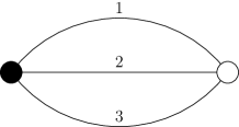
$\sum_{i_{a}}\overline{T}_{i_{1},i_{2},i_{3}}T_{i_{1}i_{2}i_{3}}$

(a) Dipole graph (Gaußian measure).

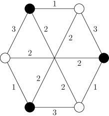
$\sum_{i_{a},\,j_{b},\,k_{c}}\overline{T}_{i_{1}i_{2}i_{3}}\overline{T}_{j_{1}j_{2}j_{3}}\overline{T}_{k_{1}k_{2}k_{3}}T_{i_{1}k_{2}j_{3}}T_{j_{1}i_{2}k_{3}}T_{k_{1}j_{2}i_{3}}$

(b) Degree 6 interaction.

Figure 1: Some bubble invariants.

Let us note that we do not restrict ourselves to connected bubbles, though the invariant of a disconnected bubble factorizes over its connected components. In the particular case $D=2$, connected bubble invariants are defined by a single even integer, the number $n$ of edges, and are just traces of power of the matrix $MM^{\dagger}$, $\operatorname{Tr}_{{\cal B}}(M,\overline{M})=\operatorname{Tr}(MM^{\dagger})^{n/2}$. In this case, non connected bubbles correspond to product of traces, also known as multitrace operators.

A polynomial invariant potential for a rank $D$ tensor is defined by summing over a finite set of $D$-bubbles, each weighted by a complex number $\lambda_{\cal B}$, called its coupling constant,

$$V(T,\overline{T})=\sum_{{\cal B}}\frac{\lambda_{\cal B}}{C_{\cal B}}\operatorname{Tr}_{\cal B}(\overline{T},T).$$ (2.2)

$C_{\cal B}$ is a combinatorial factor introduced for later convenience. It is the cardinal of the group of transformation of edges and vertices that preserve the bubble. In this paper, we mostly stay at a formal level, i.e., we expand the functional integral (1.1) in power series of the couplings using Gaußian integration. In this case, the couplings can be any complex numbers but if we require the partition function and the expectation values to be real, then we have to take the couplings to be real. At a nonperturbative level, the main difficulty lies in the fact that the trace invariants $\operatorname{Tr}_{\cal B}(\overline{T},T)$ are not necessarily positive, except for a few special cases, like the quartic models studied in [27]. When these invariant are positive, positive couplings lead to a well defined integral. In the general case, it may be useful to consider purely imaginary couplings in such a way that the exponential of the interaction term remain bounded.

There is a single quadratic trace invariant up to a factor. It is associated to the dipole, a bubble made of two vertices connected by $D$ edges, see Fig. 1. Its trace invariant reads

$$\operatorname{Tr}_{\text{dipole}}(T,\overline{T})=\sum_{i_{1}\cdots i_{D}\atop\overline{i}_{1},\dots,\overline{i}_{D}}\overline{T}_{\overline{i}_{1},\dots,\overline{i}_{D}}T_{i_{1}\cdots i_{D}}=\overline{T}\cdot T.$$

It is used to construct the normalised Gaußian measure

$$d\mu_{C}(T,\overline{T})={\cal N}\exp\big{\{}{-}\big{(}t^{-1}\overline{T}\cdot T\big{)}\big{\}}dTd\overline{T},$$

where ${\cal N}$ is a normalisation factor and $dTd\overline{T}$ the standard Lebesgue measure on the space of components of the tensors $T$ and $\overline{T}$. Then, the covariance of the Gaußian measure is simply $C_{i_{1},\dots,i_{D}|\overline{i}_{1},\dots,\overline{i}_{D}}=t\delta_{i_{1}\overline{i}_{1}}\cdots\delta_{i_{D}\overline{i}_{D}}$, which means that

$$\int d\mu_{C}(T,\overline{T})T_{i_{1}\dots i_{D}}\overline{T}_{\overline{i}_{1}\dots\overline{i}_{D}}=t\,\delta_{i_{1}\overline{i}_{1}}\cdots\delta_{i_{D}\overline{i}_{D}}$$ (2.3)

for positive $t$.

By the same token, invariant observables are also labelled by $D$-bubbles,

$${\cal O}(T,\overline{T})=\sum_{{\cal B}}\frac{{\cal O}_{\cal B}}{C_{\cal B}}\operatorname{Tr}_{\cal B}(\overline{T},T).$$

Thus, we reduce the computation of the expectation value of an observable to that of an invariant bubble. Moreover, bubble interactions may be used to generate expectations of bubble observables,

$$\langle\operatorname{Tr}_{\cal B}(\overline{T},T)\rangle =\frac{1}{Z}\frac{\partial}{\partial J_{B}}\int d\mu_{C}(T,\overline{T})\exp\left\{-V(T,\overline{T})+\sum_{{\cal B}^{\prime}}{{J}_{\cal B^{\prime}}}\operatorname{Tr}_{{\cal B}^{\prime}}(\overline{T},T)\right\}\Bigg{|}_{J_{{\cal B}^{\prime}}=0}$$

$$=\frac{\partial}{\partial J_{B}}\log Z\big{|}_{J_{{\cal B}^{\prime}}=0}.$$ (2.4)

Alternatively, any bubble observable can be expanded in powers of the components of the tensors. Thus, the basic object to compute is the expectation value of a product of components

$$\big{\langle}T_{i_{1,1}\dots i_{1,D}}\cdots T_{i_{n,1}\dots i_{n,D}}\quad\overline{T}_{\overline{i}_{1,1}\dots\overline{i}_{1,D}}\cdots\overline{T}_{\overline{i}_{n,1}\dots\overline{i}_{n,D}}\big{\rangle}.$$ (2.5)

In analogy with quantum field theory, these expectation values are referred to as correlation functions. Because of $\text{U}(1)$ invariance, correlation functions vanish if there is not an equal number of $T$ and $\overline{T}$.

Although we restrict ourselves to invariant tensor models, in the more general case of noninvariant tensors, the sum over bubbles invariants in (2.2) may be replaced by

$$V(T,\overline{T})=\sum_{{\cal B}}\prod_{\text{edges}}\sum_{i_{e},\,\overline{i}_{e}\atop\text{edge indices}}\frac{\lambda_{\cal B}\left\{i_{e},\overline{i}_{e}\right\}}{C_{\cal B}}$$

$$\hphantom{V(T,\overline{T})=}{}\times\prod_{\overline{v}\atop\text{black vertices }}\overline{T}_{\overline{i}_{\overline{v},1},\dots,\overline{i}_{\overline{v},D}}\prod_{{v}\atop\text{white vertices }}{T}_{{i}_{{v},1},\dots,{i}_{{v},D}}\prod_{e\atop\text{edges}}\delta_{\overline{i}_{e},\overline{i}_{\overline{v}(e),c(e)}}\delta_{i_{e},i_{v(e),c(e)}}.$$ (2.6)

The invariant potential (2.2) is recovered for

$$\lambda_{\cal B}\left\{i_{e},\overline{i}_{e}\right\}=\lambda_{\cal B}\prod_{e\,\text{edges}}\delta_{\overline{i}_{e},\overline{i}_{e}}.$$

The motivation behind the choice (2.6) lies in the fact that it is covariant under the group $\text{U}(N)\times\cdots\times U(N)$: it is invariant under simultaneous transformations of $\lambda_{\cal B}\left\{i_{e},\overline{i}_{e}\right\}$ and the tensors $T$ and $\overline{T}$. Moreover, this general construction renders the transition to group field theory more transparent.

2.2 Perturbative expansion

Let us now give the basic features of the expansion of an arbitrary bubble observable as a formal power series in the bubble couplings ${\lambda}_{\cal B}$. Using (2.4), we reduce such a computation to that of the partition function, considered as a function of the bubble couplings,

$$Z=\int d\mu_{C}(T,\overline{T})\exp\left\{-\sum_{{\cal B}}\frac{\lambda_{\cal B}}{C_{\cal B}}\,\operatorname{Tr}_{\cal B}(\overline{T},T)\right\}.$$

To proceed, we expand the exponential and integrate over the tensors using Wick’s theorem with the covariance (2.3). The latter can be formulated as the computation of the Gaußian expectation value of the product of $n$ pairs of a tensor and its complex conjugate

$$\int d\mu_{C}(T,\overline{T})\ T_{i_{1,1}\dots i_{1,D}}\cdots T_{i_{n,1}\dots i_{n,D}}\ \overline{T}_{\overline{i}_{1,1}\dots\overline{i}_{1,D}}\cdots\overline{T}_{\overline{i}_{n,1}\dots\overline{i}_{n,D}}$$

$$\qquad{}=t\sum_{\sigma\in\mathfrak{S}_{n}}\prod_{1\leq k\leq D}\delta_{i_{1,k},\overline{i}_{\sigma(1),k}}\cdots\delta_{i_{n,k},\overline{i}_{\sigma(n),k}}.$$

The sum over all permutations $\mathfrak{S}_{n}$ is nothing but the familiar sum over all pairings, with the constraint that a tensor is paired with its complex conjugate. The Gaußian expectation value of a product of $n$ tensors $T$ with $\overline{n}$ tensors $\overline{T}$ vanishes when $n\neq\overline{n}$.

Applying Wick’s theorem to any monomial obtained by expanding the potential amounts to summing over all contractions of $T$ with $\overline{T}$. Any such contraction corresponds to the contraction of a pair of vertices of different colours in a bubble, defined as follows. Consider a bubble ${\cal B}$, which may be disconnected, as is the case if it arises from two different bubble couplings or from a single bubble coupling associated with a disconnected bubble. Choose a white vertex $v$ and black vertex $\overline{v}$ in ${\cal B}$ and remove them, leaving a set of coloured half edges. Then, reattach the half edges respecting the colours. The resulting bubble is denoted by ${\cal B}/{\overline{v}v}$. It is convenient to materialise the choice of the pair of vertices in ${\cal B}$ before contraction by an extra colour 0 edge, represented by a dashed line, see Fig. 2. Note that if the pairs of vertices are already connected by $k$ edges in ${\cal B}$, then the pair contraction yields $k$ circles, so that we have an extra factor of $N^{k}$ resulting from the summation over the $k$ indices.

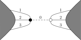
$\qquad\rightarrow\qquad$

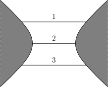
(a) Generic vertices.

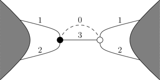
$\qquad\rightarrow\qquad$

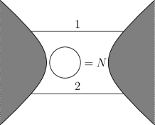
(b) Connected vertices.

Figure 2: Contraction of a pair of vertices.

Accordingly, the perturbative expansion of the partition function can be represented as a sum over $(D{+}1)$-bubbles (see Fig. 3 for an example of such a bubble)

$$Z=\int d\mu_{C}(T,\overline{T})\exp\left\{-\sum_{{\cal B}}\frac{\lambda_{\cal B}}{C_{\cal B}}\,\operatorname{Tr}_{\cal B}(\overline{T},T)\right\}=\sum_{{\cal G}\atop(D{+}1)\text{-bubbles}}\frac{N^{F({\cal G})}t^{E(G)}}{C_{\cal G}}\prod_{{\cal B}\subset{\cal G}}(-\lambda_{\cal B}).$$

This expression is obtained by contracting all pairs of vertices, thus yielding $(D{+}1)$-bubbles once we represent the pair contractions by a colour 0 line. The pair contractions can be used, in any order, to successively reduce the bubbles to a disjoint union of circles, each of them yielding a factor of $N$. On the bubble ${\cal G}$, it can be viewed as the total number of faces with colour $0$. Recall that a face of colours $0$ and $k$ is a connected subgraph of ${\cal G}$ obtained by removing all colours except $0$ and $k$. $E({\cal G})$ is the number of colour 0 edges of ${\cal G}$. The bubbles ${\cal B}\subset{\cal G}$ are simply the $D$-bubbles we started with. On the example of Fig. 3, the 3-bubble in the potentials have been drawn on a shaded disc, there is one disconnected 3-bubble (two dipoles) considered as a single interaction in the potential, whose contribution to the potential is

$$\frac{1}{2}\lambda_{\includegraphics[width=14.22636pt]{Krajewski-Fig01a}\includegraphics[width=14.22636pt]{Krajewski-Fig01a}}\big{(}\overline{T}\cdot T\big{)}^{2}.$$

The 4-bubble of Fig. 3 is 0-connected but not connected.

In many cases, it is useful to consider the logarithm of $Z$. The latter is expanded over $0$-connected bubbles,

$$\log Z=\sum_{{\cal G}\atop 0\text{-connected}\,(D{+}1)\text{-bubbles}}\frac{N^{F({\cal G})}t^{E({\cal G)}}}{C_{\cal G}}\prod_{{\cal B}\subset{\cal G}}(-\lambda_{\cal B}),$$ (2.7)

where a bubble is said to be 0-connected if the graph (with only colour 0 lines) obtained by contracting all the bubbles ${\cal B}\subset{\cal G}$ is connected. A bubble may be 0-connected without being connected if some of the bubbles ${\cal B}\subset{\cal G}$ are disconnected.

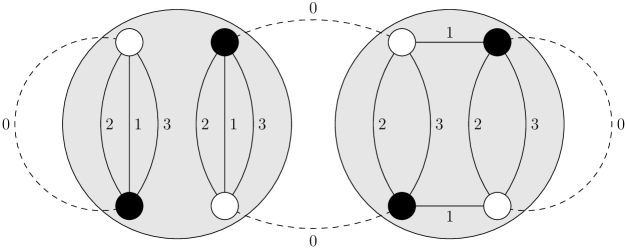
Figure 3: A 0-connected bubble with color $0$ edges and two 3-bubbles.

This expansion can be given a geometrical interpretation that may be used in discretised approaches to quantum gravity and random geometry. Each bubble ${\cal G}$ with $D+1$ colors represents a coloured triangulation of a space of dimension $D$. Its simplices of dimension $D$ are the vertices of ${\cal G}$ attached along their $D-1$ faces following the edges of ${\cal G}$. Thus, the expansion of the logarithm of the partition function (2.7) provides a sum over coloured triangulations. If all the bubbles in the potential are connected, then $\log Z$ provides us with a sum over connected triangulations. For instance, the dipole graph represents a triangulation of a sphere by 2 simplices, see Fig. 4.

$\Leftrightarrow$ 

Figure 4: Triangulation of a 3d sphere with 2 tetrahedra.

Triangulations with boundaries are represented by correlation functions, see (2.5). $(D{+}1)$-bubbles contributing to a correlation with $n$ tensors $T$ and $\overline{T}$ have $2n$ colour 0 external legs. Such a bubble ${\cal B}$ gives rise to the boundary bubble $\partial{\cal B}$. Vertices of $\partial{\cal B}$ are external legs of ${\cal B}$. They are connected by an edge of colour $k$ if and only if the two external legs belong to a face of colour $0k$ in ${\cal B}$. Recall that in a coloured tensor models a face of colours $i_{1}\dots i_{k}$ in a bubble is a connected component of the subgraph made of edges of colours $i_{1}\dots i_{k}$ in ${\cal B}$.

2.3 Tensorial group field theories

Tensorial group field theories are particular quantum field theories defined on $D$ copies of a group, usually $\text{SU}(2)$, $\text{U(1)}^{d}$, ${\mathbb{R}}^{d}$ or $\text{SL}(2,{\mathbb{C}})$. They are constructed in analogy with tensor models, we replace tensors by functions of $D$ copies of the group,

$$T_{i_{1},\dots,i_{D}}\rightarrow\Phi(g_{1},\dots,g_{D}),\qquad\overline{T}_{\overline{i}_{1},\dots,\overline{i}_{D}}\rightarrow\overline{\Phi}(\overline{g}_{1},\dots,\overline{g}_{D}).$$

Note that $\overline{g}$ is not the complex conjugate of $g$ but an independent group element that is an argument of the complex conjugate field $\overline{\Phi}$. In quantum gravity applications, $D$ denotes the space-time dimension and the group is the Lorentz group, the euclidian group or their universal covers. The group field $\Phi(g_{1},\dots,g_{D})$ represents a $D-1$ simplex and the group variables $g_{1},\dots,g_{D}$ are associated with its $D$ $(D{-}1)$-faces, see Fig. 5.

Figure 5: The group field as a tetrahedron.

In many models, the group elements are related to the normals of the tetrahedron. Then, it is assumed that they obey a closure constraint. The closure condition is implemented as an invariance of the field under left translation,

$$\Phi(g_{1},\dots,g_{D})=\Phi(hg_{1},\dots,hg_{D}),\qquad\overline{\Phi}(\overline{g}_{1},\dots,\overline{g}_{D})=\overline{\Phi}(\overline{h}\overline{g}_{1},\dots,\overline{h}\overline{g}_{D}).$$ (2.8)

for every group elements $h$ and $\overline{h}$. The covariance is defined by the Gaußian integration

$$\int d\mu_{C}(\Phi,\overline{\Phi})\,\Phi(g_{1},\dots,g_{D})\overline{\Phi}(\overline{g}_{1},\dots,\overline{g}_{D})=C\big{(}g_{1}\overline{g}^{-1}_{1},\dots,g_{D}\overline{g}^{-1}_{D}\big{)},$$

and the integration of $\Phi\,\Phi$ and $\overline{\Phi}\,\overline{\Phi}$ vanishes. Because of the closure constraint (2.8), the covariance obeys

$$C\big{(}\big{\{}g_{e}\overline{g}_{e}^{-1}\big{\}}\big{)}=C\big{(}\big{\{}hg_{e}\overline{g}_{e}^{-1}\overline{h}^{-1}\big{\}}\big{)}.$$

Note that it is also invariant under a global translation for every colour, since it only depends on products $g_{e}\overline{g}_{e}^{-1}$. The covariance propagates a tetrahedron, in analogy with the quantum field theory propagation of a particle, see Fig. 6.

Figure 6: Propagation of a tetrahedron.

A suitable covariance may be constructed using the heat kernel on the group $H_{\alpha}$,

$$C_{\Lambda,\Lambda_{0}}\big{(}\big{\{}g_{e}\overline{g}_{e}^{-1}\big{\}}\big{)}=\int_{\frac{1}{\Lambda_{0}^{2}}}^{\frac{1}{\Lambda^{2}}}d\alpha\int dhd\overline{h}\prod_{1\leq i\leq D}H_{\alpha}\big{(}hg_{i}\overline{g}_{i}^{-1}\overline{h}^{-1}\big{)}.$$ (2.9)

$\Lambda$ and $\Lambda_{0}$ are cut-offs that have to be introduced to avoid divergences. Group integrations are performed using the Haar measure and implement the required invariances.

As for the tensor models, the general interaction potential can also be expanded over $D$-bubbles. However, in this case there is no reason to impose unitary invariance. Therefore, we use the general form of the bubble couplings (2.6), replacing tensor indices by group elements,

$$V(\Phi,\overline{\Phi})=\sum_{{\cal B}}\frac{1}{C_{\cal B}}\int\prod_{e}dh_{e}\prod_{v,i}d{g_{v,i}}\prod_{\overline{v},\overline{i}}d\overline{g}_{\overline{v},\overline{i}}\lambda_{\cal B}(\{h_{e}\})\prod_{e}\delta\big{(}h_{e}^{-1}g_{v(e),c(e)}(\overline{g}_{\overline{v}(e),c(e)})^{-1}\big{)}$$

$$\hphantom{V(\Phi,\overline{\Phi})=}{}\times\prod_{\overline{v}\atop\text{black vertices }}\overline{\Phi}(\overline{g}_{\overline{v},1},\dots,\overline{g}_{\overline{v},D})\prod_{{v}\atop\text{white vertices }}{\Phi}(g_{{v},1},\dots,g_{{v},D}),$$ (2.10)

where $\delta$ is the Dirac distribution on the group, defined by $\int dg\delta(g)f(g)=f(1)$. Note that we have imposed translation invariance, so that the couplings only depend on the products $g_{v(e),c(e)}(\overline{g}_{\overline{v}(e),c(e)})^{-1}$

Then, the perturbative expansion yields a sum over triangulations of dimension $D$, weighted by certain graph amplitudes. By a suitable choice of the bubble couplings $\lambda_{\cal B}(\{h_{e}\})$, one can show that this amplitude can be made equal to a spin foam amplitude. Indeed, a spin foam is 2-complex and can be constructed from the $(D{+}1)$-bubbles by adding a 2-cell to any colour $0k$ face, for every $k$.

2.4 Couplings in the spin network basis

The relation to spin foam models can be made more precise if we formulate the theory in terms of spins $j$ (labelling representations of $\text{SU}(2)$) and intertwiners $\iota$ (invariant tensors) in the case of $\text{SU}(2)$. Then, we expand the bubble couplings using the Peter–Weyl theorem,

$$\lambda_{\cal B}(\{h_{e}\})=\sum_{j_{e}\,\text{spins}\atop i_{v}\,\text{intertwiners}}\lambda_{\cal B}(\{j_{e},\iota_{v}\})\prod_{e}d_{j_{e}}$$

$${}\times\prod_{e\,\text{edges}}\Bigg{\{}\!\!\sum_{m_{v,k},\,\overline{m}_{\overline{v},k}\atop\text{magnetic indices}}\!\!\!(\iota_{v(e)})_{m_{v(e),1}\dots m_{v(e),D}}{\cal D}^{j_{e}}_{m_{v(e),c(e)},\overline{m}_{\overline{v}(e),c(e)}}(h_{e})(\overline{\iota}_{\overline{v}(e)})_{\overline{m}_{\overline{v}(e),1}\dots\overline{m}_{v(e),D}}\Bigg{\}}.$$

${\cal D}_{\overline{m}m}^{j}(h)$ are the Wigner matrices with $d_{j}=2j+1$ the dimension of the spin $j$ representation and the intertwiner appear because of the closure constraint (2.8). The intertwiners are invariant tensors in the tensor product of representation of edges incident to a vertex, following the ordering provided by the colours. They are chosen so that they define a orthonormal basis in this tensor product. The new couplings $\lambda_{\cal B}(\{j_{e},\iota_{v}\})$ depend on the choice of a spin for every edge and of an intertwiner for every vertex. Such a representation theoretic data defines a spin nertwork $s$, so that the couplings can be simply indexed by a spin network. For example, for the dipole graph, the spin network formulation yields

$$\lambda_{\includegraphics[width=11.38092pt]{Krajewski-Fig01a}}(h_{1},h_{2},h_{3})=\sum_{j_{1},\,j_{2},\,j_{3},\,\iota}\lambda_{\includegraphics[width=11.38092pt]{Krajewski-Fig01a}}(j_{1},j_{2},j_{3},\iota)$$

$$\hphantom{\lambda_{\includegraphics[width=11.38092pt]{Krajewski-Fig01a}}(h_{1},h_{2},h_{3})=}{}\times\sum_{m_{1},\,m_{2},\,m_{3}\atop\overline{m}_{1},\,\overline{m}_{2},\,\overline{m}_{3}}\iota_{m_{1}m_{2}m_{3}}D_{m_{1}\overline{m}_{1}}^{j_{1}}(h_{1})D_{m_{2}\overline{m}_{2}}^{j_{2}}(h_{2})D_{m_{3}\overline{m}_{3}}^{j_{3}}(h_{3})\overline{\iota}_{\overline{m}_{1}\overline{m}_{2}\overline{m}_{3}}.$$

This can be considered as a non-Abelian Fourier transform,

$$\text{position space: $h_{e}$}\qquad\leftrightarrow\qquad\text{momentum space: $j_{e}$, $\iota_{v}$.}$$

Moreover, it is important to realise that the existence of the intertwiner between representations labelled by spins puts some constraints on these spins. For instance, for three spins $j_{1}$, $j_{2}$, $j_{3}$, there exists an intertwiner (and it is then unique up to normalisation) if and only if the triangular inequality $|j_{1}-j_{2}|\leq j_{3}\leq j_{1}+j_{2}$ is satisfied.

3 Exact renormalisation group equations

3.1 Wilson’s ideas in quantum field theory

Let us start with a heuristic overview of Wilson’s idea in quantum field theory, deferring a more precise formulation till the next section. Consider a quantum field theory with an action $S_{0}$ and a UV cut-off $\Lambda_{0}$. The basic object of interest is the generating functional of correlation functions,

$$Z[J]=\int[D\phi]_{\Lambda_{0}}\exp\{-S_{0}[\phi]+J\phi\},$$

where $[D\phi]_{\Lambda_{0}}$ is a measure that integrates only over fields with momenta $\lesssim\Lambda_{0}$.

Wilson’s idea amounts to performing this integration not in a single step but in a series of partial integrations. The cutoff $\Lambda_{0}$ is then reduced to a lower cutoff $\Lambda$ by integrating the modes between $\Lambda$ and $\Lambda_{0}$. The low energy physics, for instance correlation functions for fields at momenta $\lesssim\Lambda$ is then left unchanged. Denoting by $\phi_{0}$ the original field with modes less than $\Lambda_{0}$, $\phi$ a field with modes less than $\Lambda$ and by $\chi$ the remaining degrees of freedom between $\Lambda$ and $\Lambda_{0}$,

$$\phi_{0}=\phi+\chi.$$

This separation of modes translates into the following equation for the generating functional

$$Z[J] =\int[D\phi_{0}]_{\Lambda_{0}}\exp\{-S_{0}[\phi_{0}]+J\phi_{0}\}$$

$$=\int[D\phi]_{\Lambda}[D\chi]_{\Lambda,\Lambda_{0}}\exp\{-S_{0}[\phi+\chi]+J\phi+J\chi\}$$

$$=\int[D\phi]_{\Lambda}\exp\{-S_{\Lambda}[\phi]+J\phi\},$$

where we have used $J\chi=0$ since we are only interested in the low energy correlation functions. $S_{\Lambda}$ is the Wilsonian effective action at scale $\Lambda$ defined by

$$S_{\Lambda}[\phi]=-\log\int[D\chi]_{\Lambda,\Lambda_{0}}\exp\{-S_{0}[\phi+\chi]\}.$$

This procedure leads to a flow equation for the effective action

$$\Lambda\frac{dS_{\Lambda}}{d\Lambda}=\beta(\Lambda,S_{\Lambda}),$$ (3.1)

with the initial condition $S_{\Lambda_{0}}=S_{0}$.

The physics of this equation is best captured by expanding the effective action in local operators, which are monomials of the fields and their derivatives. Writing symbolically $O[\partial^{d},\phi^{n}]$ such a monomial with $n$ occurrences of the field and $d$ derivatives, the action reads, in a space-time of dimension $D$,

$$S_{\Lambda}[\phi]=\sum_{i\atop\text{local operators}}\int d^{D}x\,g_{i}(\Lambda)O\big{[}\partial^{d_{i}},\phi^{n_{i}}\big{]}.$$

The flow equation for the effective action (3.1) translates into a system of equations for the couplings,

$$\Lambda\frac{dg_{i}}{d\Lambda}=\beta_{i}(\Lambda,\{g_{j}\}).$$

It is convenient to write this equation in terms of dimensionless couplings $u_{i}(\Lambda)$, related to $g_{i}(\Lambda)$ by

$$g_{i}(\Lambda)=\Lambda^{\delta_{i}}u_{i}(\Lambda),$$

where $\delta_{i}$ is the canonical dimension of the local operator $i$. Assuming translational invariance, this dimension is

$$\delta_{i}=D-n_{i}\left(\frac{D}{2}-1\right)-d_{i}.$$

Dimensional analysis allows us to write the flow equation for dimensionless couplings as

$$\Lambda\frac{du_{i}}{d\Lambda}=-\delta_{i}u_{i}+\beta_{i}(\{u_{j}\}).$$

Couplings are classified according to the sign of their dimension:

• relevant couplings with $\delta_{i}>0$,

• irrelevant couplings with $\delta_{i}<0$,

• marginal couplings with $\delta_{i}=0$.

In the vicinity of the Gaußian fixed point $u^{\ast}_{i}=0$ (i.e., in perturbation theory), the physical consequences of this equation are the following:

• Universality: Whatever the irrelevant couplings at scale $\Lambda_{0}$ are (provided $u_{i}(\Lambda_{0})$ are bounded, so that $g_{i}(\Lambda_{0})\sim\Lambda_{0}^{\delta_{i}}$ goes to zero for large $\Lambda_{0}$), when $\Lambda_{0}\rightarrow\infty$, the couplings at scale $\Lambda$ are attracted towards a manifold that can be parametrized by the relevant and marginal couplings only.

• Renormalisability: When $\Lambda_{0}\rightarrow\infty$ with $\Lambda$ fixed, the relevant and marginal couplings at scale $\Lambda$ diverge. Perturbative renormalisation amounts to imposing their values at $\Lambda$ by a measurement. Then, all the other operators can be computed at scale $\Lambda$ in terms of the relevant and marginal operators at scale $\Lambda$, in the limit $\Lambda_{0}\rightarrow\infty$.

This provides a rationale for renormalisation: When renormalisable couplings (i.e., couplings with $\delta_{i}\geq 0$) are available, the latter dominate the low energy behaviour in the limit $\Lambda_{0}\rightarrow\infty$. Low energy physics can be formulated in terms of low energy parameters. Of course, when no such couplings exist, for instance if they are forbidden by symmetries, the limit $\Lambda_{0}\rightarrow$ cannot be taken.

These statements can be rigorously proved in perturbation theory, see [35]. Obviously, a nonperturbative study is required, especially when marginal couplings are involved or when no renormalisable couplings are available. It may also be that the theory is attracted towards a nontrivial fixed point. Finally, let us mention that these ideas also play a prominent role in constructive physics. The latter aims at a nonperturbative construction of the theory based on a multiscale analysis of the Feynman graphs [37].

3.2 Exact renormalisation group equations

In order to understand how the previous ideas can be implemented in tensor models and tensorial group field theories, a more precise formulation is required. Within this section, we remain in the general setting of a quantum field theory. In order to keep the notations as simple and universal as possible, we write fields as $\phi^{i}$, where $i$ may be a discrete index, a space-time index or a momentum. We separate the action into a quadratic part and an interaction potential $V_{0}[\phi]$. The quadratic part is included into a Gaußian measure of covariance $C(t,t_{0})$ which we assume to be written as an integral

$$C(t,t_{0})=\int_{t_{0}}^{t}ds\,K(s).$$ (3.2)

The interacting part of effective action is defined as

$$V(t,\phi)=-\log\int d\mu_{C(t,t_{0})}(\chi)\exp\{-V_{0}(t,\phi+\chi\},$$ (3.3)

with the initial condition $V(t_{0},\phi)=V_{0}[\phi]$ since $C(t_{0},t_{0})=0$ so that there is no integration.

The effective interaction $V(t,\phi)$ obey the semi-group relation, see [43],

$$Z =\int d\mu_{C(t,t_{0})}[\phi]\exp\{-V_{0}(t,\phi)\}$$

$$=\int d\mu_{C(t,t_{1})}[\phi]\int d\mu_{C(t_{1},t_{0})}(\chi)\exp\{-V_{0}(\phi+\chi)\}$$

$$=\int d\mu_{C(t,t_{1})}[\phi]\exp\{-V(t_{1},\phi)\}.$$

Then, the integration over an infinitesimal shell with $t_{1}=t-dt$ leads to the following differential equation, known as Polchinski’s exact renormalisation group equation,

$$\frac{\partial V}{\partial t}=\frac{1}{2}\sum_{i,j}K_{ij}(t)\left(-\frac{\partial V}{\partial\phi^{i}}\frac{\partial V}{\partial\phi^{j}}+\frac{\partial^{2}V}{\partial\phi^{i}\partial\phi^{j}}\right).$$ (3.4)

At the perturbative level, the effective potential (3.3) can be expanded over Feynman graphs using the background field technique. $\phi$ dependent vertices are introduced by expanding $V_{0}(\phi+\chi)$ in powers of $\chi$. Then, Feynman graphs are generated by integrating over $\chi$. Then, the flow equation provides a recursive construction of these graphs by successively adding edges. The first term corresponds to a tree edge (between two connected components) and the second one to a loop edge (within the same connected component), see Fig. 7.

${\displaystyle\frac{\partial}{\partial t}}$    = -${\displaystyle\frac{1}{2}}$    +${\displaystyle\frac{1}{2}}$ 

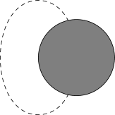
Figure 7: A graphical interpretation of the Polchinski’s equation.

While Polchinski’s equation is a powerful tool in the perturbative case, in nonperturbative investigations (for instance search for nontrivial fixed points using truncations), it is often more convenient to sum the contributions of the trees. This is achieved by introducing the Legendre transform $\Gamma$ of $V$ with respect to some sources. Alternatively $\Gamma$ can be defined in analogy with (3.3) by

$$\Gamma(t,\phi)=-\log\int d\mu_{C(t,t_{0})}(\chi)\exp\left\{-V_{0}(t,\phi+\chi)+\frac{\partial\Gamma}{\partial\phi}\cdot\chi\right\}.$$

It obeys the following differential equation, known as Wetterich’s equation, which we write symbolically as

$$\frac{\partial\Gamma}{\partial t}=\frac{1}{2}\operatorname{Tr}\left[C^{-1}KC^{-1}\left(1+C\frac{\partial^{2}\Gamma}{\partial\phi\partial\phi}C\right)^{-1}\right],$$ (3.5)

which has to be understood as a geometrical series for the matrix products

$$\sum_{j,k}C_{ij}\frac{\partial^{2}\Gamma}{\partial\phi_{j}\partial\phi_{k}}C_{kl}.$$

Wetterich’s equation is particularly useful in the search for fixed points. A fixed point is an effective action such $\beta(S_{\ast})=0$. Because $\Lambda\frac{dS}{d\Lambda}=\beta(S)$, a fixed point action describes a scale invariant theory. These fixed points play an important role in statistical physics. In the case of the $O(N)$ invariant model in three dimensions, the long distance behavior at a second order phase transition is governed by a infrared stable fixed point (i.e., with only few divergent directions), known as the Wilson–Fisher fixed point. In this case the ultraviolet cut-off $\Lambda_{0}$ is fixed because it is nothing but the inverse lattice spacing. The vicinity of the critical point is described by this fixed point in the long distance limit $\Lambda\ll\Lambda_{0}$. On the other side, ultraviolet stable fixed point may allow the large cut-off limit $\Lambda_{0}\rightarrow\infty$ in theories of fundamental interactions. Asymptotically free theories provide natural examples with a Gaußian fixed point but more general fixed points have been found in some simple models, like the $D=3$ Gross–Neveu model, see for instance [11]. Then, physical theories are parametrised by the few coordinates on the stable manifold. Such a scenario, known as ”asymptotic safety”, has been proposed by Weinberg and may allow to construct a quantum theory of gravity with only field theoretical degrees of freedom. We refer the reader to the reviews [3, 36, 39] for more complete overviews of these renormalisation group equations.

The field theory case presented in the previous section is recovered by taking $t=\log(\Lambda/\Lambda_{\text{ref}})$, where $\Lambda_{\text{ref}}$ is an immaterial reference scale that disappears from the equations. Then, $C_{t_{0},t}=C_{\Lambda_{0},\Lambda}$ smoothly integrates out modes between $\Lambda$ and $\Lambda_{0}$. In momentum space, it can be written as

$$C(\Lambda_{0},\Lambda,p,q)=\delta(p+q)\int_{\Lambda}^{\Lambda_{0}}\frac{d\Lambda^{\prime}}{\Lambda^{\prime}}K(\Lambda^{\prime},p).$$

Sources can be included in $V$ for convenience since we assume that they decouple from the high energy behaviour. When formulated in momentum space, the flow equation (3.4) for a translationally invariant field theory takes the form

$$\Lambda\frac{dS}{d\Lambda}=\frac{1}{2}\int d^{D}p\,K(\Lambda,p)\left(-\frac{\delta V}{\delta\phi(p)}\frac{\delta V}{\delta\phi(-p)}+\frac{\delta^{2}V}{\delta\phi(p)\delta\phi(-p)}\right).$$

Expanding the effective interaction in powers of the field

$$V[\Lambda,\phi]=\sum_{n}\frac{1}{n!}\int dp_{1}\cdots dp_{n}\delta(p_{1}+\cdots+p_{n})G_{n}(\Lambda,p_{1},\dots,p_{n})\phi(p_{1})\cdots\phi(p_{n})$$

yields the system of equations

$$\frac{\partial G_{n}}{\partial\Lambda}(\Lambda,p_{1},\dots,p_{n})=\frac{1}{2}\int d^{D}p\,K(\Lambda,p)\bigg{(}\sum_{i=0}^{n}\big{\{}-G_{i+1}(\Lambda,p,p_{1},\dots,p_{i})$$

$$\hphantom{\frac{\partial G_{n}}{\partial\Lambda}(\Lambda,p_{1},\dots,p_{n})=}{}\times G_{n-i+1}(\Lambda,-p,p_{i+1},\dots,p_{n})+G_{n+2}(\Lambda,p,-p,p_{1},\dots,p_{n})\big{\}}\bigg{)}.$$ (3.6)

Then, dimensional analysis can be done by further expanding $G_{n}$ in powers of the momenta.

The next sections are devoted to an implementation of these ideas in the context of tensor models and tensorial group field theories, following our presentation in [32].

3.3 Polchinski’s equation for invariant tensor models

Let us first consider an analogue of the Polchinski’s exact renormalisation group equation (3.4) for random tensors. We consider a covariance $C(t,t_{0})$ such that (3.2). The effective potential is defined as in (3.3),

$$V(t,T,\overline{T})=-\log\int d\mu_{C(t,t_{0})}(T^{\prime},\overline{T}^{\prime})\exp\big{\{}{-}V_{0}\big{(}t,T+T^{\prime},\overline{T}+\overline{T}^{\prime}\big{)}\big{\}}.$$

Since we treat $T$ and $\overline{T}$ as independent variables, the flow equation for the effective potential (3.4) takes the form

$$\frac{\partial V}{\partial t}=\sum_{i_{1},\dots,i_{D}\atop\overline{i}_{1},\dots,\overline{i}_{D}}K_{i_{1},\dots,i_{D}|\overline{i}_{1},\dots,\overline{i}_{D}}(t)\left(-\frac{\partial V}{\partial T_{i_{1},\dots,i_{D}}}\frac{\partial V}{\partial\overline{T}_{\overline{i}_{1},\dots,\overline{i}_{D}}}+\frac{\partial^{2}V}{\partial T_{i_{1},\dots,i_{D}}\partial\overline{T}_{\overline{i}_{1},\dots,\overline{i}_{D}}}\right).$$ (3.7)

In order to preserve unitary invariance (2.1), the covariance has to be diagonal, see (2.3). In this section, we restrict our attention to

$$C_{i_{1},\dots,i_{D}|\overline{i}_{1},\dots,\overline{i}_{D}}(t,t_{0})=\mathfrak{K}(t-t_{0})\prod_{1\leq k\leq D}\delta_{i_{k},\overline{i}_{k}},$$

with $\mathfrak{K}$ independent of $t$ and $t_{0}$. Although simple, such a covariance is not really in accordance with the spirit of Wilson’s ideas. It would be better to choose a covariance that gradually reduces the size of the tensors by integrating over some of its components. For simplicity, we restrict ourselves to an invariant integration. We refer to [20, 21] for an application of a reduction of the size to matrix models suing Wetterich’s equation.

In the unitary invariant case, we expand the interaction potential over bubbles as in (2.2)

$$V(t,T,\overline{T})=\sum_{{\cal B}}\frac{\lambda_{\cal B}(t)}{C_{\cal B}}\operatorname{Tr}_{\cal B}(\overline{T},T),$$ (3.8)

with couplings that depend on the parameter $t$ controlling the flow.

Polchinski’s exact renormalisation group equation for tensors (3.7) involves the operations of deriving $V$ with respect to $T$ and $\overline{T}$. At the level of bubble couplings, they respectively amount to removing a white vertex $v$ and a black vertex $\overline{v}$. Then, the contraction with the derivative of the covariance $K$ connects the resulting edges respecting the colours. Therefore, when acting on bubble couplings in $V$,

$$\sum_{i_{1},\dots,i_{D}\atop\overline{i}_{1},\dots,\overline{i}_{D}}K_{i_{1},\dots,i_{D}|\overline{i}_{1},\dots,\overline{i}_{D}}(t)\left(-\frac{\partial V}{\partial T_{i_{1},\dots,i_{D}}}\frac{\partial V}{\partial\overline{T}_{\overline{i}_{1},\dots,\overline{i}_{D}}}+\frac{\partial^{2}V}{\partial T_{i_{1},\dots,i_{D}}\partial\overline{T}_{\overline{i}_{1},\dots,\overline{i}_{D}}}\right)$$

is equivalent to a contraction of a pair of vertices, either on two independent couplings (first term) or on the same coupling (second term). At the dual level of triangulation, the flow equation can be represented graphically as in Fig. 8.

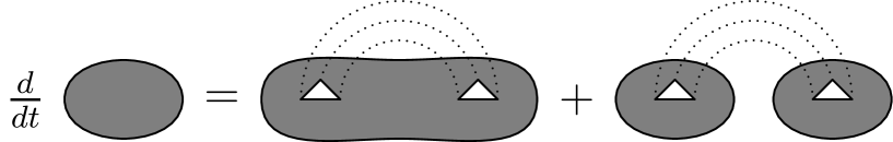
Figure 8: Dual interpretation of the flow equation for $D=3$.

Equation (3.7) translates into a system of equations for the couplings $\lambda_{\cal B}$. To explicit this system, it is useful to introduce the inverse operation of a pair contraction, which is called a cut. A $k$-cut $c$ in a bubble ${\cal B}$ is defined as a subset of edges $\{e_{1},\dots,e_{k}\}$ of ${\cal B}$ with different colours. The cut bubble ${\cal B}_{c}$ is the bubble obtained from ${\cal B}$ by cutting the $k$ edges $\{e_{1},\dots,e_{{k}}\}$ into half-edges, attaching to them a new black $\overline{v}$ and a new white vertex $v$ and joining $v$ and $\overline{v}$ by $D-k$ edges carrying the colors not in $\{e_{1},\dots,e_{k}\}$. Then, it follows that ${\cal B}/{v\overline{v}}={\cal B}_{c}$. The notion of $k$-cut with $k\neq D$ is necessary to deal with the contraction of a pair that is connected by $D-k$ edges.

This ensures that ${\cal B}_{c}$ is a bubble with $D$ colours. In particular, if $c$ is a 0-cut, ${\cal B}_{c}$ is just the disjoint union of ${\cal B}$ with a dipole. A 1-cut on an edge $e$ is just the insertion on $e$ of a pair of vertices joined by $D-1$ edges carrying the colours different from that of $e$.

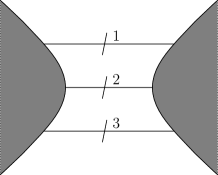
$\quad\rightarrow\quad$

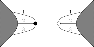
(a) A 3-cut.

$\quad\rightarrow\quad$

(b) A 2-cut.

Figure 9: Examples of cut operations.

Substituting the bubble expansion (3.8) into the flow equation (3.7), we arrive at the system of differential equations governing the bubble couplings. Thus, the evolution of the couplings reads

$$\frac{\partial\lambda_{\cal B}}{\partial t}=\mathfrak{K}\sum_{k=0}^{D}\sum_{k\text{-cut }c}N^{D-k}\lambda_{B_{c}}-\mathfrak{K}\sum_{D\text{-cut }c\atop{\kappa({\cal B}_{c})>\kappa({\cal B})}}\sum_{{\cal B}^{\prime},{\cal B}^{\prime\prime}\atop{\cal B}_{c}={\cal B}^{\prime}\cup{\cal B}^{\prime\prime},\,v\in{\cal B}^{\prime},\,\overline{v}\in{\cal B}^{\prime\prime}}\lambda_{\cal B^{\prime}}\lambda_{\cal B^{\prime\prime}},$$

In this equation, the sum runs over $k$-cuts $c$ for $0\leq k\leq D$. The second term involves a summation over $D$-cut that increases the number of connected components $\kappa({\cal B})$ of ${\cal B}$ and over ways of writing ${\cal B}_{c}$ as a disjoint union of a bubble ${\cal B}^{\prime}$ containing $v$ and a bubble ${\cal B}^{\prime\prime}$ containing $\overline{v}$. Finally, let us emphasize that even if the initial potential $V_{0}$ does not contain nonconnected bubbles, the latter are generated by the loop-like term in the flow equation. Furthermore, they play a key role in the large $N$ limit.

3.4 Large $\boldsymbol{N}$ melonic universality

In order to study the large $N$ limit, we make a change of variables in the couplings,

$${\lambda}_{{\cal B}}(t)=N^{\delta(\cal B)}u_{\cal B}(t).$$

$\delta({\cal B})$ has to be determined in such a way that the rescaled variables $u_{{\cal B}}$ are of order unity in $N$. The latter play the role of the dimensionless variables in the Wilsonian approach to quantum field theory, with $\delta$ analogous to the canonical dimension of a coupling. This amounts to parametrising the potential as

$$V(t,T,\overline{T})=\sum_{{\cal B}}\frac{N^{\delta(\cal B)}u_{\cal B}(t)}{C_{\cal B}}\,\operatorname{Tr}_{\cal B}(\overline{T},T).$$

This change of variables factorizes the leading order behaviour of the bubble couplings in the large $N$ limit.

Since the covariance involves the dipole and the latter could as well be considered as an interaction, invariance under shifts of part of the covariance into the interaction requires that the constant $\mathfrak{K}$ be written as $\mathfrak{K}=N^{\delta(\includegraphics[width=14.22636pt]{Krajewski-Fig01a})}$. In a more general discussion, a multiplicative factor that admits a finite limit when $N\rightarrow\infty$ could be included. For our purposes, this is irrelevant and we choose this constant to be 1. In the renormalisation group language, this number can be considered as a finite, cut-off independent wave function renormalisation and can be removed by a constant rescaling of the fields.

The couplings $u_{{\cal B}}$ are finite at large $N$ if the obey a renormalisation group equation involving only negative powers of $N$,

$$\frac{\partial u_{{\cal B}}}{\partial t}=\beta_{0}(\{u_{\cal B^{\prime}}\})+\frac{1}{N}\beta_{1}(\{u_{\cal B^{\prime}}\})+\frac{1}{N^{2}}\beta_{2}(\{u_{\cal B^{\prime}}\})+\cdots,$$

so that in the large $N$ limit the couplings $u_{{\cal B}}$ are finite and solely determined by $\beta_{0}$. To determine $\delta({\cal B})$ such that this is the case, let us assume that it is of the form

$$\delta({\cal B})=\alpha+\beta\kappa({\cal B})+\gamma v({\cal B}),$$

where $\kappa({\cal B})$ is the number of connected components of the bubble ${\cal B}$ and $v({\cal B})$ its total number of vertices. It is not necessary to introduce the number of edges since $e({\cal B})=\frac{D}{2}v({\cal B})$, but more refined numbers could be used, like the number of faces. Then, the renormalisation group equation reads

$$\frac{\partial u_{\cal B}}{\partial t}=\sum_{k=0}^{D}\sum_{k\text{-cut }c}N^{\delta({\cal B}_{c})+D-k-\delta({\cal B})-\delta(\includegraphics[width=14.22636pt]{Krajewski-Fig01a})}u_{B_{c}}$$

$$\hphantom{\frac{\partial u_{\cal B}}{\partial t}=}{}-\sum_{D\text{-cut }c\atop{\kappa({\cal B}_{c})>\kappa({\cal B})}}\sum_{{\cal B}^{\prime},{\cal B}^{\prime\prime}\atop{\cal B}_{c}={\cal B}^{\prime}\cup{\cal B}^{\prime\prime},\,v\in{\cal B}^{\prime},\,\overline{v}\in{\cal B}^{\prime\prime}}N^{\delta({\cal B}^{\prime})+\delta({\cal B}^{\prime\prime})-\delta({\cal B})-\delta(\includegraphics[width=14.22636pt]{Krajewski-Fig01a})}u_{\cal B^{\prime}}u_{\cal B^{\prime\prime}},$$

Note that for the dipole $\delta(\includegraphics[width=14.22636pt]{Krajewski-Fig01a})=\alpha+\beta+2\gamma$. Then, the tree-like term (second term in the previous equation) is independent of $N$ because $v({\cal B})=v({\cal B}^{\prime})+v({\cal B}^{\prime\prime})-2$ and $\kappa({\cal B})=\kappa({\cal B}^{\prime})+\kappa({\cal B}^{\prime\prime})-1$. The power of $N$ in the loop-like term (first term in the previous equation) can be written as

$$\delta({\cal B}_{c})+D-k-\delta({\cal B})-\delta(\includegraphics[width=14.22636pt]{Krajewski-Fig01a}) =D-\alpha-k-\beta\kappa({\cal B},c),$$ (3.9)

where $\kappa({\cal B},c)$ is defined as the number of connected components of ${\cal B}$ containing edges of the cut, except for a $D$-cut that increases the number of connected components of ${\cal B}$, in which case $\kappa({\cal B},c)=0$. This implies that $\kappa({\cal B}_{c})=\kappa({\cal B})-\kappa({\cal B},c)+1$. This exponent is negative if we choose $\alpha=D$ and $\beta=-1$ with $\gamma$ arbitrary, but other choices are possible, see the discussion in [9]. Then, the renormalisation group equation is

$$\frac{\partial u_{\cal B}}{\partial t}=\sum_{k=0}^{D}\sum_{k\text{-cut }c}N^{\kappa({\cal B},c)-k}u_{B_{c}}-\sum_{D\text{-cut }c\atop{\kappa({\cal B}_{c})>\kappa({\cal B})}}\sum_{{\cal B}^{\prime},{\cal B}^{\prime\prime}\atop{\cal B}_{c}={\cal B}^{\prime}\cup{\cal B}^{\prime\prime},\,v\in{\cal B}^{\prime},\,\overline{v}\in{\cal B}^{\prime\prime}}u_{\cal B^{\prime}}u_{\cal B^{\prime\prime}}.$$ (3.10)

We always have $k\geq\kappa({\cal B},c)$ and $k=\kappa({\cal B},c)$ if and only if all edges of the cut belong to different connected components of ${\cal B}$. In particular, this holds for any 0-cut and any 1-cut. The evolution equations for low order bubble couplings are given in Appendix A.1 for $D=3$ and in Appendix A.2 for $D=4$.

Since the exponent of $N$ in (3.10) is negative, the limit $N\rightarrow\infty$ can be taken. For matrices ($D=2$), the large $N$ limit is equivalent to the equation derived in [22].

In this regime, only $D$-cuts that disconnect the graph or $k$-cuts with each edge in distinct connected components (including the 0-cuts) survive. Staring with the empty bubble coupling $u_{\varnothing}$, that corresponds to $\log Z$, only melonic bubbles are generated when solving iteratively (3.10) in powers of $t-t_{0}$. Recall that a bubble ${\cal M}$ is said to be melonic if, for every white vertex $v$, there is a black vertex $\overline{v}$ such that the removal of $v$ and $\overline{v}$ increases the number of connected components by $D-1$.

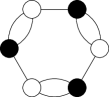
(a) Melonic bubbles.

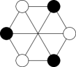
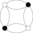
(b) Non melonic bubbles.

Figure 10: Melonic and nonmeloinc bubbles for $D=3$ and $D=4$.

Consequently, there is a kind of melonic universality: Whatever the initial couplings $u_{\cal B}(t_{0})$ are, the large $N$ partition function only depends on the melonic couplings $u_{\cal M}(t_{0})$. Thus, as far as the partition function is concerned, nonmelonic bubbles are irrelevant. The partition function is all we need to compute the expectation value of a bubble since

$$\big{\langle}\operatorname{tr}_{\cal B}(T,\overline{T})\rangle=-\frac{1}{N^{D-\kappa({\cal B})}}\frac{\partial}{\partial u_{\cal B}(t_{0})}\log Z=N^{\kappa({\cal B})}\frac{\partial u_{\varnothing}(t)}{\partial u_{\cal B}(t_{0})},$$

since $\log Z=-N^{D}u_{\varnothing}(t)$. If ${\cal B}$ is melonic, the derivative $\frac{\partial u_{\varnothing}(t)}{\partial u_{\cal B}(t_{0})}$ is of order unity. If ${\cal B}$ is not melonic, then it is suppressed by negative powers $N$. Taking the second derivative of $\log Z$ shows that the expectation value of a product of melonic bubbles factorizes at leading order. The actual computation of this expectation value is performed in Section 4.4. Note that the melonic universality holds for any $D$, including the matrix model case $D=2$, for which all interactions are melonic. However, the Gaußian ansatz presented in Section 4.4 does not hold for matrices. These techniques also allow to show the large $N$ Gaußian nature of the correlation functions for random tensors, see [32].

Finally, let us emphasize that our treatment is perturbative: The partition and the expectation values of observables are considered as formal power series in the initial couplings $u_{\cal B}(t_{0})$ and the large $N$ limits holds order by order. It is not excluded that small $1/N$ contributions add up and alter the scaling exponents at a nonperturbative level. This could happen, for instance, by resuming contributions to the dipole graph, thus leading to a nontrivial wave function renormalisation.

3.5 Group field theory

We consider now tensorial group field theories, analogous to tensor models, provided we replace rank $D$ tensors by functions over $D$ copies of a group $G$,

$$T_{i_{1},\dots,i_{D}}\rightarrow\Phi(g_{1},\dots,g_{D}),\qquad\overline{T}_{\overline{i}_{1},\dots,\overline{i}_{D}}\rightarrow\overline{\Phi}(\overline{g}_{1},\dots,\overline{g}_{D}).$$

As already emphasized, $\overline{g}$ is not the complex conjugate of $g$ but an independent group element that is an argument of the complex conjugate field $\overline{\Phi}$. The covariance includes both a UV cut off $\Lambda_{0}$ and an IR one $\Lambda$ (see (2.9)), and depends on the $D$ products of group elements $g_{i}\overline{g}_{i}^{-1}$,

$$C\big{(}\Lambda,\Lambda_{0},\big{\{}g_{i}\overline{g}_{i}^{-1}\big{\}}\big{)}=\int_{\frac{1}{\Lambda_{0}^{2}}}^{\frac{1}{\Lambda^{2}}}d\alpha K\big{(}\alpha,\big{\{}g_{i}\overline{g}_{i}^{-1}\big{\}}\big{)},$$

so that

$$\Lambda\frac{\partial C}{\partial\Lambda}\big{(}\Lambda,\Lambda_{0},\big{\{}g_{i}\overline{g}_{i}^{-1}\big{\}}\big{)}=-\frac{2}{\Lambda^{2}}K\left(\frac{1}{\Lambda^{2}},\big{\{}g_{i}\overline{g}_{i}^{-1}\big{\}}\right).$$

In the following general discussion, $K(\alpha,\{g_{i}\overline{g}_{i}^{-1}\})$ is left unspecified. It is often convenient to take it as a product of $D$ heat kernels averaged over the group. The general interaction can be expanded in terms of bubble couplings (see (2.10)),

$$V(\Lambda,\Phi,\overline{\Phi})=\sum_{{\cal B}}\frac{1}{C_{\cal B}}\int\prod_{e}dg_{v(e),c(e)}d\overline{g}_{\overline{v}(e),c(e)}$$

$${}\times\lambda_{\cal B}\big{(}\Lambda,\big{\{}g_{v(e),c(e)}(\overline{g}_{\overline{v}(e),c(e)})^{-1}\big{\}}\big{)}\!\!\!\!\prod_{\overline{v}\atop\text{black vertices }}\!\!\!\!\overline{\Phi}(\overline{g}_{\overline{v},1},\dots,\overline{g}_{\overline{v},D})\!\!\!\!\prod_{{v}\atop\text{white vertices }}\!\!\!\!{\Phi}(g_{{v},1},\dots,g_{{v},D}),$$

where the bubble couplings only depend on $g_{v(e),c(e)}\overline{g}^{-1}_{\overline{v}(e),c(e)}$ because of the global translation invariance.

For group field theories, Polchinski’s exact renormalisation group equation reads (see the tensor model analogue (3.7))

$$\Lambda\frac{\partial V}{\partial\Lambda}=-\frac{2}{\Lambda^{2}}\int\prod_{1\leq i\leq D}dg_{i}d\overline{g}_{i}$$

$$\hphantom{\Lambda\frac{\partial V}{\partial\Lambda}=}{}\times K\left(\frac{1}{\Lambda^{2}},\big{\{}g_{i}\overline{g}_{i}^{-1}\big{\}}\right)\left(-\frac{\delta V}{\delta\Phi(\{g_{i}\})}\frac{\delta V}{\delta\overline{\Phi}(\{\overline{g}_{\overline{i}}\})}+\frac{\delta^{2}V}{\delta{\Phi}(\{{g}_{i}\})\delta\overline{\Phi}(\{\overline{g}_{i}\})}\right).$$ (3.11)

Let us determine the system of equations satisfied by the bubble couplings $\lambda_{\cal B}$. These involve $k$-cuts $c$ on the edges of ${\cal B}$. Recall that a $k$-cut is a subset of $k$ edges of distinct colours, with $i_{1},\dots,i_{D-k}$ the colours of the edge not in the cut. We cut these edges, attach two new vertices $\overline{v}_{c}$ and $v_{c}$ and complete the graph by connecting these vertices by $D-k$ edges $e_{i_{1}},\dots,e_{i_{k}}$ carrying the colours not in the cut. We denote by ${\cal B}_{c}$ the resulting bubble and, if $k=D$ and if ${\cal B}_{c}$ has one more connected component than ${\cal B}$, ${\cal B}^{{}^{\prime}}_{c}$ and ${\cal B}^{{}^{\prime\prime}}_{c}$ are any bubbles such that ${\cal B}_{c}={\cal B}^{{}^{\prime}}_{c}\cup{\cal B}^{{}^{\prime\prime}}_{c}$ with $v_{c}\in{\cal B}^{{}^{\prime}}_{c}$ and $\overline{v}_{c}\in{\cal B}^{{}^{\prime\prime}}_{c}$.

Then, inserting the expansion of $V$ in terms of bubble couplings (2.10) in the exact renormalisation group equation (3.11) and identifying the contribution of a bubble on both sides lead to

$$\Lambda\frac{\partial\lambda}{\partial\Lambda}\big{(}\big{\{}g_{v(e),c(e)}(\overline{g}_{\overline{v}(e),c(e)})^{-1}\big{\}}\big{)}=-\frac{2}{\Lambda^{2}}\int\prod_{1\leq i\leq D}dg_{i}d\overline{g}_{i}K\left(\frac{1}{\Lambda^{2}},\big{\{}g_{i}\overline{g}_{i}^{-1}\big{\}}\right)$$

$$\hphantom{\Lambda\frac{\partial\lambda}{\partial\Lambda}\big{(}\big{\{}g_{v(e),c(e)}(\overline{g}_{\overline{v}(e),c(e)})^{-1}\big{\}}\big{)}=}{}\times\Bigg{\{}\sum_{0\leq k\leq D}\sum_{c}\lambda_{{\cal B}_{c}}\big{(}\Lambda,\big{\{}g_{v(e),c(e)}(\overline{g}_{\overline{v}(e),c(e)})^{-1}\big{\}}_{e\in{\cal B}},g_{i},\overline{g}_{i}\big{)}$$

$$\hphantom{\Lambda\frac{\partial\lambda}{\partial\Lambda}\big{(}\big{\{}g_{v(e),c(e)}(\overline{g}_{\overline{v}(e),c(e)})^{-1}\big{\}}\big{)}=}{}-\!\!\!\sum_{c\text{$D$-cut}\atop\text{ disconnecting ${\cal B}$}}\sum_{{\cal B}_{c}^{{}^{\prime}}\cup{\cal B}_{c}^{{}^{\prime\prime}}}\!\!\lambda_{{\cal B}_{c}^{{}^{\prime}}}\big{(}\Lambda,\big{\{}g_{v(e),c(e)}(\overline{g}_{\overline{v}(e),c(e)})^{-1}\big{\}}_{e\in{\cal B}_{c}^{{}^{\prime}}},g_{i}\big{)}$$

$$\hphantom{\Lambda\frac{\partial\lambda}{\partial\Lambda}\big{(}\big{\{}g_{v(e),c(e)}(\overline{g}_{\overline{v}(e),c(e)})^{-1}\big{\}}\big{)}=}{}\times\lambda_{{\cal B}_{c}^{{}^{\prime\prime}}}\big{(}\Lambda,\big{\{}g_{v(e),c(e)}(\overline{g}_{\overline{v}(e),c(e)})^{-1}\big{\}}_{e\in{\cal B}_{c}^{{}^{\prime\prime}}},\overline{g}_{i}\big{)}\Bigg{\}}.$$ (3.12)

This expression is not very illuminating, but interesting consequences can be drawn from it in specific models. In the next two sections, we investigate the case of Abelian models with closure constraints and $\text{SU}(2)$ models in the spin network basis.

3.6 Scaling and renormalisation for Abelian models with closure constraint

In this section, we consider Abelian models based on the group $\text{U(1)}^{d}$. Elements of U(1) are written as $g=\exp{2\text{i}\pi\frac{\theta}{L}}$ with $\theta\in[0,L]$, with $L$ being a length. The covariance is of heat kernel type

$$C(\Lambda,\Lambda_{0},\{\theta_{i}-\overline{\theta}_{i}\})=\int_{\frac{1}{\Lambda_{0}^{2}}}^{\frac{1}{\Lambda^{2}}}d\alpha\sum_{\{p_{i}\}\in{\frac{1}{L}\mathbb{Z}}^{dD}}\exp\left(-\left\{\alpha\sum_{1\leq i\leq D}p_{i}^{2}+\text{i}\sum p_{i}(\theta_{i}-\overline{\theta}_{i})\right\}\right)\delta_{\sum p_{i},0},$$

where we have enforced the condition $\sum_{i}p_{i}=0$ so that the closure constraint is fulfilled.

The exact renormalisation group equation written in terms of bubble couplings (3.12) is

$$\Lambda\frac{\partial\lambda_{\cal B}(\left\{p_{e}\right\})}{\partial\Lambda}=-\frac{2}{\Lambda^{2}}\sum_{k=0}^{D}\sum_{k\text{-cut }c}\sum_{\{p_{l}\}_{l\notin c}}\exp\left(-\frac{1}{\Lambda^{2}}\left\{\sum_{i=1}^{D}p_{i}^{2}\right\}\right)\lambda_{B_{c}}(\{p_{e}\}_{e\in{\cal B}},\{p_{l}\}_{l\notin c})\delta_{\sum\limits_{i=1}^{D}p_{i},0}$$

$${}+\frac{2}{\Lambda^{2}}\!\!\sum_{D\text{-cut }c\atop\kappa({\cal B}_{c})>\kappa({\cal B})}\sum_{{\cal B}^{\prime},{\cal B}^{\prime\prime}\atop{{\cal B}_{c}={\cal B}^{\prime}\cup{\cal B}^{\prime\prime},\atop v\in{\cal B}^{\prime},\,\overline{v}\in{\cal B}^{\prime\prime}}}\!\!\!\!\!\exp\left(\!-\frac{1}{\Lambda^{2}}\left\{\sum_{i=1}^{D}p_{i}^{2}\right\}\!\right)\lambda_{\cal B^{\prime}}(\{p_{e}\}_{e\in{\cal B^{\prime}}})\lambda_{\cal B^{\prime\prime}}(\{{p}_{e}\}_{e\in{\cal B}^{\prime\prime}})\delta_{\sum\limits_{i=1}^{D}p_{i},0}.\!\!\!$$ (3.13)

This equation is the group field theory analogue of (3.6) in the framework of quantum field theory. Note that because of the closure constraint, the bubble couplings are only defined on subspaces of momentum space such that the sum of momenta incident to any vertex is 0. We further assume $L$ to be large enough ($1/L\ll\Lambda$) so that momenta can be treated as continuous variables. Then we can trade sums for integrals

$$\sum_{p}\rightarrow L^{d}\int dp\qquad\text{and}\qquad\delta_{\sum{p_{i}},0}\rightarrow L^{-d}\delta\left(\sum{p_{i}}\right).$$

Otherwise, a more precise but cumbersome analysis can be performed using the Poisson resummation. Finally, we also allow derivatives of the bubble couplings with respect to momenta and impose rotational invariance in momentum space. This last hypothesis is fulfilled if we assume that the initial couplings are invariant under rotation since the propagator is.

To understand the large $\Lambda$ behaviour, we repeat the steps followed in Section 3.4. Let us introduce the analogue of dimensionless bubble couplings $u_{\cal B}$ defined by

$$\lambda_{\cal B}(\{p_{e}\},\Lambda)=\Lambda^{\delta({\cal B})}u_{\cal B}(\{q_{e}\},\Lambda)\qquad\text{with}\qquad p_{e}={\Lambda}{q_{e}}.$$

$\delta({\cal B})$ is not the dimension as would be derived by rescaling all lengths, $L$ included. It is merely a scaling dimension for large $\Lambda$ that encodes the dominant behaviour of $\lambda_{{\cal B}}$.

In terms of these new couplings, the exact renormalisation group equation (3.13) is

$$\Lambda\frac{\partial u_{\cal B}(\{q_{e}\})}{\partial\Lambda}=-\delta({\cal B})\,u_{\cal B}(\{q_{e}\})+\sum_{e}q_{e}\frac{\partial u_{\cal B}(\{q_{e}\})}{\partial q_{e}}-2\sum_{k=0}^{D}\sum_{0\leq k\leq D\atop c\,k\text{-cut }}\frac{\Lambda^{\delta({\cal B}_{c})-\delta({\cal B})-2+d(D-k)-d}}{L^{d-d(D-k)}}$$

$${}\times\int\prod_{l\notin c}dq_{l}\exp\left\{-\left(\sum_{i}q_{i}^{2}\right)\right\}u_{B_{c}}(\{q_{e}\}_{e\in{\cal B}},\{q_{l}\}_{l\notin c})\delta\left(\sum_{i}q_{i}\right)$$

$${}+2\sum_{D\text{-cut }c\atop\kappa({\cal B}_{c})>\kappa({\cal B})}\sum_{{\cal B}_{c}={\cal B}^{\prime}\cup{\cal B}^{\prime\prime},\atop v\in{\cal B}^{\prime},\,\overline{v}\in{\cal B}^{\prime\prime}}\!\!\!\frac{\Lambda^{\delta({\cal B}^{\prime})+\delta({\cal B}^{\prime\prime})-\delta({\cal B})-2}}{L^{d}}\exp\left\{-\left(\sum_{i}q_{i}^{2}\right)\right\}u_{\cal B^{\prime}}(\{q_{e}\}_{e\in{\cal B^{\prime}}})u_{\cal B^{\prime\prime}}(\{{q}_{e}\}_{e\in{\cal B}^{\prime\prime}}).$$

Suppose that this equation can be written with only negative powers of $\Lambda$,

$$\Lambda\frac{\partial u_{{\cal B}}}{\partial\Lambda}=\beta_{0}(\{u_{\cal B}^{\prime}\})+\frac{1}{\Lambda}\beta_{1}(\{u_{\cal B}^{\prime}\})+\frac{1}{\Lambda^{2}}\beta_{2}(\{u_{\cal B}^{\prime}\})+\cdots.$$

Then, the large $\Lambda$ behaviour is entirely governed (at least in perturbation theory) by $\beta_{0}$. To this aim, let us search for a suitable scaling dimension for the bubble interactions in the form

$$\delta({\cal B})=\alpha+\beta\kappa({\cal B})+\gamma v({\cal B}).$$

The exponent in the tree-like term is

$$\delta({\cal B}^{\prime})+\delta({\cal B}^{\prime\prime})-\delta({\cal B})-2=\alpha+\beta+2\gamma-2,$$

while for the loop like term it is

$$\delta({\cal B}_{c})-\delta({\cal B})-2+d(D-k)-d=-dk-\beta\kappa({\cal B},c)+\beta+2\gamma-2+d(D-1).$$

We recall that $\kappa({\cal B},c)$ is defined as the number of connected components of ${\cal B}$ containing edges of the cut, except for a $D$-cut that increases the number of connected components of ${\cal B}$, in which case $\kappa({\cal B},c)=0$. It obeys $\kappa({\cal B}_{c})=\kappa({\cal B})-\kappa({\cal B},c)+1$.

Setting $\alpha=d(D-1)$, $\beta=-d$, and $2\gamma=-d(D-2)+2$, the exponent of the tree-like term vanishes while the loop-like one it is $d(\kappa({\cal B},c)-k)$, thus always negative. Therefore, the couplings $u_{\cal B}$ are governed by a flow equation that only involves negative powers of $\Lambda$. This leads to a scaling dimension

$$\delta({\cal B})=d(D-1)-d\kappa({\cal B})-(d(D-2)-2)\frac{v({\cal B})}{2}.$$

For connected bubbles, this is the scaling dimension found in [16] by Carrozza, Oriti and Rivasseau using multiscale analysis.

Assuming that the general picture presented in Section 3.1 for quantum field theory remains valid, perturbatively renormalisable interactions correspond to relevant and marginal interactions, or equivalently $\delta({\cal B})\geq 0$. This leads us to only five values of $D$ and $d$ for which such interactions can be found. Indeed, if we also take into account the term associated with rescaling of momenta,

$$\sum_{e}q_{e}\frac{\partial u_{\cal B}(\{q_{e}\})}{\partial q_{e}}$$

that is diagonalised by degree $n$ homogenous polynomials in $q_{e}$, renormalisable terms are characterised by

$$\delta({\cal B},n)=(D-1)d-\kappa({\cal B})d-[(D-2)d-2]\frac{v({\cal B})}{2}-n\geq 0.$$ (3.14)

In particular, among all the renormalisable interactions, we always have the mass term $\delta_{\includegraphics[width=14.22636pt]{Krajewski-Fig01a},0}=2$ and for the kinetic term $\delta_{\includegraphics[width=14.22636pt]{Krajewski-Fig01a},2}=0$.

Let us end by listing all renormalisable interactions in Abelian models with a closure constraint. The condition $\delta({\cal B})\geq 0$ implies $v({\cal B})\leq 2+\frac{4}{d(D-2)-2}$. Non trivial interactions involve bubbles with at most four vertices, so that we are left with only two possibilities: $d(D-2)=4$ and $d(D-2)=3$, which leads to the following 5 renormalisable theories. This list, with connected interactions only, was first obtained in [16] using the multiscale analysis of Feynman graphs.

• $D=3$ and $d=4$ so that $\delta=8-4\kappa-v$. The renormalisable interactions is quartic and melonic

  

  ($\delta=0$).

  The fixed point structure of a non-Abelian version of this model has been studied in [14].

• $D=4$ and $d=2$ so that $\delta=6-2\kappa-v$. The renormalisable interactions are quartic

  

  ($\delta=0$),   ($\delta=0$).

  Note that the second interaction is not melonic (called necklace in [9]).

• $D=6$ and $d=1$ so that $\delta=5-\kappa-v$. The renormalisable interactions are quartic

  

  ($\delta=0$),   ($\delta=0$),    ($\delta=0$).

  The last two interactions are not melonic. This model was shown to be renormalisable in [41, 33] and its fixed point structure was further investigated in [7].

• $D=3$ and $d=3$ so that $\delta=6-3\kappa-v/2$. The renormalisable interactions are quartic and sextic

  

  ($\delta=1$),   ($\delta=0$),    ($\delta=0$),   ($\delta=0$).

  The first term is in fact superrenormalisable ($\delta>0$) and the last one is not melonic. Its non-Abelian counterpart is the tensorial SU(2) group field theory in $D=3$ which corresponds to three-dimensional Euclidian quantum gravity without the cosmological constant, first shown to be renormalisable in [16].

• $D=5$ and $d=1$ so that $\delta=4-\kappa-v/2$. The renormalisable interactions are quartic and sextic. We first have the melonic ones

  

  ($\delta=1$),   ($\delta=0$),    ($\delta=0$),   ($\delta=0$).

  The last interaction is not connected ($\kappa=2$). This model, with the nonconnected interaction, was shown to be renormalizable in [41]. Besides, there are also nonmelonic renormalisable interactions.

Note that all these bubble couplings with $v\geq 4$ have dimension 0 or 1, so that there is no possibility of adding a derivative coupling. Indeed, the latter corresponds to a term with $n>0$ in (3.14), which would lead to a negative dimension, the case $n=1$ being forbidden by rotational symmetry. Of course, we could always add quadratic terms (mass and kinetic terms) to the list of interaction. Then, the kinetic term can play the role of a derivative coupling.

It is also worthwhile to notice that some of the renormalisable interactions are not necessary melonic. As for unitarily invariant random tensors, nonmelonic interactions appear with a negative power of $\Lambda$ in the flow of renormalisable melonic interactions. Therefore, they do not require renormalisation if the bare theory only contains melonic interactions. However, if the bare theory contains nonmelonic renormalisable interactions, the latter requires renormalisation.

3.7 $\boldsymbol{\text{SU}(2)}$ models in the spin network basis

In the $\text{SU}(2)$ case which is involved in many spin-foam models, it is possible to expand all the bubble couplings on spin networks, see [31], rather than just bubbles. For the group $\text{SU}(2)$, spin network observables provide a nice basis. We work with the heat kernel

$$H\big{(}\alpha,g\overline{g}^{-1}\big{)}=\sum_{j}(2j+1)\exp\big{\{}{-}\alpha j(j+1)\big{\}}\sum_{-j\leq m\leq j}{\cal D}^{j}_{mm}\big{(}g\overline{g}^{-1}\big{)}.$$

The covariance is obtained by averaging over the group

$$C\big{(}\Lambda,\Lambda_{0},\big{\{}g_{i}\overline{g}_{i}^{-1}\big{\}}\big{)}=\sum_{j_{1}\dots j_{D}\,\text{spins}\atop\iota\,\text{intertwiner}}\Bigg{(}\sum_{m_{1},\dots,m_{D}\atop\overline{m}_{1},\dots,\overline{m}_{D}}\iota_{m_{1},\dots,m_{D}}{\cal D}^{j_{1}}_{m_{1}\overline{m}_{1}}\big{(}g_{1}\overline{g}_{1}^{-1}\big{)}\cdots$$

$${}\times{\cal D}^{j_{D}}_{m_{D}\overline{m}_{D}}\big{(}g_{D}\overline{g}_{D}^{-1}\big{)}\overline{\iota}_{\overline{m}_{1},\dots,\overline{m}_{D}}d_{j_{1}}\cdots d_{j_{D}}\exp\big{(}{-}\alpha\big{\{}j_{1}(j_{1}+1)+\cdots+j_{D}(j_{D}+1)\big{\}}\big{)}\Bigg{)},$$

where we performed the group averaging thanks to the relation

$$\int dh{\cal D}_{m_{1}m^{\prime}_{1}}^{j_{1}}(h)\cdots{\cal D}_{m_{D}m^{\prime}_{D}}^{j_{D}}(h)=\sum_{\iota}\iota_{m_{1}\dots m_{D}}\overline{\iota}_{m^{\prime}_{1}\dots m^{\prime}_{D}}.$$

Then, the spin network formulation of (3.12) is

$$\Lambda\frac{\partial\lambda_{\cal B}(\{j_{e},\iota_{v}\})}{\partial\Lambda}=-\frac{2}{\Lambda^{2}}\sum_{0\leq k\leq D\atop c\,k\text{-cut }}\sum_{\iota}\sum_{\{j_{l}\}_{l\notin c}}\prod_{l}d_{j_{l}}\exp\left(-\frac{1}{\Lambda^{2}}\left\{\sum_{i=1}^{D}j_{i}(j_{i}+1)\right\}\right)$$

$${}\times\lambda_{B_{c}}(\{j_{e}\}_{e\in{\cal B}},\{j_{l}\}_{l\notin c},\{i_{v}\}_{v\in{\cal B}},\iota)+\frac{2}{\Lambda^{2}}\!\!\sum_{D\text{-cut }c\atop\kappa({\cal B}_{c})>\kappa({\cal B})}\!\!\sum_{\iota}\!\!\!\sum_{{\cal B}^{\prime},{\cal B}^{\prime\prime}\atop{{\cal B}_{c}={\cal B}^{\prime}\cup{\cal B}^{\prime\prime},\atop v\in{\cal B}^{\prime},\,\overline{v}\in{\cal B}^{\prime\prime}}}\!\!\!\!\exp\left(-\frac{1}{\Lambda^{2}}\left\{\sum_{i=1}^{D}j_{i}(j_{i}+1)\right\}\right)$$

$${}\times\lambda_{\cal B^{\prime}}(\{j_{e^{\prime\prime}}\}_{e^{\prime\prime}\in{\cal B^{\prime}}}\{\iota_{v^{\prime}}\}_{v^{\prime}\in{\cal B^{\prime}}},\iota)\lambda_{\cal B^{\prime\prime}}(\{j_{e^{\prime\prime}}\}_{e^{\prime\prime}\in{\cal B^{\prime\prime}}}\{\iota_{v^{\prime\prime}}\}_{v^{\prime\prime}\in{\cal B^{\prime\prime}}},\iota).$$

Let us emphasize the analogy with (3.13), the spin playing the role of the momenta. The constraint is implemented by the insertion of the interwiner $\iota$ at the two vertices created by the cut. Consequently, it acts as a constraint since we can cut some edges only if their spins admit an intertwiner. For $D=3$ this constraint is the triangle inequality. It is also interesting to note the similarity with the tensor model case, with the factor $N^{D-k}$ replaced by the product over the $D-k$ edges not in the cut of the dimensions $d_{j_{l}}$.

3.8 Wetterich’s equation and nontrivial fixed points

The search for nontrivial fixed points in group field theories have been investigated by several authors. We give here a very brief account of the rationale behind these works since they also make use of exact renormalisation group equations. We refer the reader to the original literature [4, 6, 7, 14] for the precise calculations and the phase diagrams.

These works use Wetterich’s equation (3.5) expanded as

$$\frac{\partial\Gamma}{\partial t}=\operatorname{Tr}\left[C^{-1}KC^{-1}\left(1+C\frac{\partial^{2}\Gamma}{\delta\Phi\delta\overline{\Phi}}C\right)^{-1}\right]$$

$$\hphantom{\frac{\partial\Gamma}{\partial t}}{}=\sum_{n=0}^{\infty}(-1)^{n}\operatorname{Tr}\left[C^{-1}KC^{-1}\underbrace{C\frac{\partial^{2}\Gamma}{\delta\Phi\delta\overline{\Phi}}\cdots C\frac{\partial^{2}\Gamma}{\delta\Phi\delta\overline{\Phi}}}_{\text{$n$ times}}\right].$$ (3.15)

In this framework, a heat kernel type of covariance is used and the effective average action $\Gamma$ is expanded over bubble couplings as in (2.10). Then, (3.15) is expanded a series of colour $0$ one loop graphs whose vertices are the $D$-bubbles in the expansion of $\Gamma$.

To obtain the contribution to $\frac{\partial\lambda_{\cal B}}{\partial t}$, one has to look for all possibilities of writing ${\cal B}$ as

$${\cal B}=\big{(}{\cal B}_{1}\cup\cdots\cup{\cal B}_{n}\big{)}\bigg{/}\big{(}v_{1}\overline{v}_{2},v_{2}\overline{v}_{3},\dots,v_{n-1}\overline{v}_{n},v_{n}\overline{v}_{1}\big{)},$$

where $v_{i}$ and $\overline{v}_{i}$ are respectively a white and a black vertex in ${\cal B}_{i}$. For instance, $\frac{\partial}{\partial t}\lambda_{\parbox{14.22636pt}{\includegraphics[width=14.22636pt]{Krajewski-Fig-page23a}}}$ involves a term quadratic in $\lambda_{\includegraphics[width=14.22636pt]{Krajewski-Fig-page23a}}$, see Fig. 11.

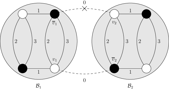
Figure 11: A contribution to the evolution of a quartic melon.

In order to write down the evolution equation of a coupling pertaining to a given bubble ${\cal B}$ in terms of all the bubbles in the chain ${\cal B}_{1},\dots,{\cal B}_{n}$, it is therefore necessary to find all such possible chains of bubbles. This is solved by the following algorithm, involving a sequence of $n$ cuts since they are the inverse of inverse operation of a contraction of a line of color 0.

1. The first cut $c_{1}$ is arbitrary and results in ${\cal B}_{c1}$, with two new vertices $v_{1}$ and $\overline{v}_{1}$. This cut determines the insertion of the derivative of the covariance $K$, materialised by a cross in Fig. 11.

2. The next cuts $c_{2},\dots,c_{n}$ must always increase the number of connected components (therefore they involve all $D$ colors) with the constraint that each new connected component contains 1 or 2 new vertices $v_{i}$ and $\overline{v}_{j}$. If the first cut has not increased the number of connected components, all the cuts have to be performed on the connected component of ${\cal B}_{c_{1}}$ containing $v_{1}$ and $\overline{v}_{1}$; otherwise they may be performed anywhere.

3. Partition the set of connected components of ${\cal B}_{c_{1}\dots c_{n}}$ into $n$ sets, each of which containing one of the white vertices and one of the black vertices previously constructed in such a way that joining corresponding vertices leads to a cycle of colour $0$ lines.

4. The $n$ sets of the partition define the $n$ bubbles ${\cal B}_{1},\dots,{\cal B}_{n}$

As is usual, for a given bubble there is a maximal value of $n$, if we exclude the trivial cuts involving all the $D$ edges incident to a given vertex. Except for the first cut, this kind of cut simply amounts to an insertion of a chain of dipoles which may be removed by a change in the propagator.

To search for fixed points, one usually resorts to truncations. It means that we select a few couplings, usually including the mass $m^{2}\overline{\Phi}\cdot\Phi$ and the kinetic term $(Z-1)\overline{\Phi}\cdot\Delta\Phi$, both associated to the dipole graph, as well as some interactions, encoded in the bubble couplings, expanded around zero momentum (in Abelian theories). For instance, in the model considered by Benedetti and Lahoche in [7] in $D=6$ with the group $\text{U}(1)$, only the interaction associated to the quartic melon given in Fig. 12 has been retained.

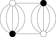
Figure 12: The quartic melon in $D=6$.

We focus now on this model and review briefly their work. In this case, the flow equations reduce to the system

$$\frac{\partial m^{2}}{\partial t}=\beta_{m^{2}}\big{(}Z,m^{2},\lambda,t\big{)},\qquad\frac{\partial Z}{\partial t}=\beta_{Z}\big{(}Z,m^{2},\lambda,t\big{)},\qquad\frac{\partial\lambda}{\partial t}=\beta\big{(}Z,m^{2},\lambda,t\big{)}.$$

The wave function renormalisation is not a coupling and one has to rescale the fields as $\Phi\rightarrow Z^{-1/2}\Phi$ and $\overline{\Phi}\rightarrow Z^{-1/2}\overline{\Phi}$ in order to have fixed points. Second, it is also necessary to rescale $m$ and $\lambda$ according to their scaling dimension for large $t$,

$${\lambda}=\text{e}^{t(6-D)}Z^{2}\overline{\lambda},\qquad{m}^{2}=\text{e}^{2t}Z\overline{m}^{2}.$$

Note that $6-D$ is the scaling dimension of the bubble found in equation (3.14), with $\Lambda\propto\text{e}^{t}$. Finally, determining $Z$ in terms of $\overline{m}$ and $\overline{\lambda}$ leads to a system of equations

$$\frac{\partial\overline{m}^{2}}{\partial t}=\overline{\beta}_{\overline{m}^{2}}\big{(}\overline{m}^{2},\overline{\lambda},t\big{)},\qquad\frac{\partial\overline{\lambda}}{\partial t}=\overline{\beta}\big{(}\overline{m}^{2},\overline{\lambda},t\big{)}.$$

Although nonautonomous (i.e., still involving $t$) because of the finite size of the group, there are fixed points in the limit $t\rightarrow\infty$. Besides the Gaußian one with $\overline{m}=0$ and $\overline{\lambda}=0$, there are two others fixed points. One of them cannot be connected to the Gaußian one by a trajectory because of the presence of a singularity. The other one has one relevant and one irrelevant direction. It corresponds to a negative value of $\overline{m}^{2}$, possibly indicating a phase transition. Similar results have been obtained by the other authors mentioned at the beginning of this section.

4 Loop equations

4.1 Reparametrisation invariance in quantum field theory

To begin with, let us consider again a general quantum field theory whose fields are collectively denoted by $\phi^{i}$. The basic object of interest is the generating function for correlation functions, which we write symbolically as

$$Z[J]=\int[D\phi]\exp\{-S[\phi]+J\phi\}.$$

In this section, we consider formal algebraic relations satisfied by the generating function, treating the field as a finite-dimensional variable for simplicity. This is enough for the heuristic purpose of this following presentation.

Because it is an integral over all fields, the generating functional $Z[J]$ must be invariant under any change of variables in the space of fields, a property known as reparametrisation invariance. Consider an infinitesimal change of variable, which we write as

$$\phi^{i}\rightarrow\phi^{i}+\epsilon X^{i}[\phi].$$

Invariance of $Z[J]$ under such a change of variable translates into the equation

$$\int[D\phi]\sum_{i}\bigg{(}\frac{\partial X^{i}}{\partial\phi^{i}}-X^{i}\frac{\partial S}{\partial\phi^{i}}+X^{i}J_{i}\bigg{)}\exp\{-S[\phi]+J\phi\}=0.$$

The first term is the Jacobian of the change of variable and the two others arise from the variation of the argument of the exponential. Since every function of the field can be obtained as a derivative acting on the source, we arrive at

$$\sum_{i}\left\{\frac{\partial X^{i}}{\partial\phi^{i}}\left(\frac{\partial}{\partial J}\Big{)}-X^{i}\Big{(}\frac{\partial}{\partial J}\right)\frac{\partial S}{\partial\phi^{i}}\left(\frac{\partial}{\partial J}\right)+J_{i}X^{i}\left(\frac{\partial}{\partial J}\right)\right\}Z[J]=0.$$ (4.1)

Introducing the differential operator

$${\cal L}_{X}=\sum_{i}\left\{\frac{\partial X^{i}}{\partial\phi^{i}}\left(\frac{\partial}{\partial J}\right)-X^{i}\left(\frac{\partial}{\partial J}\right)\frac{\partial S}{\partial\phi^{i}}\left(\frac{\partial}{\partial J}\right)+J_{i}X^{i}\left(\frac{\partial}{\partial J}\right)\right\}.$$

Invariance under reparametrisation takes the following simple form

$${\cal L}_{X}Z[J]=0.$$

Although relatively complicated, these differential operators obey a simple commutation relation

$$[{\cal L}_{X},{\cal L}_{Y}]={\cal L}_{[X,Y]}$$

with $[X,Y]$ the commutator between the two vectors fields $X$ and $Y$ defined on the space of fields

$$[X,Y]^{i}=\sum_{j}X^{j}\frac{\partial Y^{i}}{\partial\phi^{j}}-Y^{j}\frac{\partial X^{i}}{\partial\phi^{j}}.$$

$[X,Y]$ is nothing but the infinitesimal part of the commutator between the change of variables associated to $X$ and $Y$. Therefore, the operators ${\cal L}$ define a representation of the Lie algebra of infinitesimal change of variables.

When the vector field $X$ is independent of $\phi$, the associated change of variables is simply a translation in the space of fields, $\phi^{i}\rightarrow\phi^{i}+\epsilon^{i}$. Then, (4.1) takes the form

$$\left\{\frac{\partial S}{\partial\phi^{i}}\left(\frac{\partial}{\partial J}\right)+J_{i}\right\}Z[J]=0.$$

These are the Schwinger–Dyson equations. which are the quantum analogue of the equations of motion. They provide enough information to reconstruct $Z[J]$ in perturbation theory, see [43].

4.2 Loop equations for tensor models

Let us apply the general framework depicted in the previous section to unitarily invariant random tensor models. These equations where first derived by Gurau in [24] at leading order and at all orders in [26]. We follow the presentation given in [30].

We start with an interaction of the form given in (2.2), except that we do not include the combinatorial factor,

$$V(T,\overline{T})=\sum_{{\cal B}}\lambda_{\cal B}\operatorname{Tr}_{\cal B}(\overline{T},T).$$

The inclusion of the combinatorial factor $C_{T}$ is immaterial since it amounts to trading $\lambda_{\cal B}$ for $\frac{\lambda_{B}}{C_{\cal B}}$. Here, we have included all bubbles, even nonconnected ones and the empty one. The latter is simply a constant $\lambda_{\varnothing}$ that does not couple to the tensors. Then, solving the theory amounts to computing the partition function as a function of all the bubble couplings,

$$Z(\{\lambda_{\cal B}\})=\int d\mu_{C}(T,\overline{T})\exp\{-V(T,\overline{T})\},$$ (4.2)

with a diagonal covariance $C=t\,\delta_{i_{1}\overline{i}_{1}}\cdots\delta_{i_{D}\overline{i}_{D}}$. This has to be considered as a formal power series in the variables $\lambda_{\cal B}$, ordered by the number of vertices of the bubbles, in such a way that at a given order there is only a finite number of terms. The expectation value of a bubble is then obtained by

$$\big{\langle}\operatorname{Tr}_{\cal B}(\overline{T},T)\big{\rangle}=-\frac{\partial}{\partial\lambda_{\cal B}}(\log Z).$$

If only a subset of bubble couplings are present in the actual potential, all couplings not present in the potential have to be set to 0 after the derivation.

For unitarily invariant models, there is a preferred set of change of variables parametrised by bubbles with a vertex removed. Indeed, if $\overline{v}$ is a black vertex, then we define $\operatorname{Tr}_{{\cal B}\backslash\overline{v}}(\overline{T},T)$ as $\operatorname{Tr}_{{\cal B}}(\overline{T},T)$ with the tensor $\overline{T}$ at $\overline{v}$ removed. Treating $T$ and $\overline{T}$ as independent variables, the change of variables associated with ${{\cal B}\backslash\overline{v}}$ is

$$T\rightarrow T+\epsilon_{{\cal B}\backslash\overline{v}}\operatorname{Tr}_{{\cal B}\backslash\overline{v}}(\overline{T},T),\qquad\overline{T}\rightarrow\overline{T},$$ (4.3)

with $\epsilon_{{\cal B}\backslash\overline{v}}$ an infinitesimal parameter. Performing this change of variables in (4.2) leads to the identity

$$\int d\mu_{C}(T,\overline{T})\Bigg{\{}{-}t^{-1}\operatorname{Tr}_{{\cal B}}(\overline{T},T)+\sum_{v\in{\cal B}\atop\text{white vertex}}N^{l({\cal B},\overline{v},v)}\operatorname{Tr}_{{\cal B}/\overline{v}v}(\overline{T},T)$$

$$\qquad{}-\sum_{{\cal B}^{\prime}\atop v^{\prime}\in{\cal B^{\prime}}\,\text{white vertex}}\lambda_{{\cal B^{\prime}}}\operatorname{Tr}_{({\cal B}^{\prime}\cup{\cal B})/\overline{v}v^{\prime}}(\overline{T},T)\Bigg{\}}\exp\{-V(T,\overline{T})\}=0.$$

For any bubble ${\cal B}$, recall that ${\cal B}/v\overline{v}$ is the bubble with the pair of vertices $v\overline{v}$ contracted (see Fig. 2) and $l({\cal B},v,\overline{v})$ is the number of edges in ${\cal B}$ that connect $v$ and $\overline{v}$. The first two terms arise from the change of the Gaußian measure, the second one being the Jacobian. The third term comes from the change of the potential. Note that the contribution of the covariance is of the same form as that of the dipole, considered as a bubble coupling.

Writing this equation in terms of bubble expectation values, it reads

$$\big{\langle}\operatorname{Tr}_{\cal B}(T,\overline{T})\big{\rangle}=t\!\!\!\sum_{v\in{\cal B}\atop\text{white vertex}}\!\!\!\!\!N^{l({\cal B},\overline{v},v)}\big{\langle}\operatorname{Tr}_{{\cal B}/\overline{v}v}(\overline{T},T)\big{\rangle}-t\!\!\!\sum_{{\cal B}^{\prime}\,v^{\prime}\in{\cal B^{\prime}}\atop\text{white vertex}}\!\!\!\!\!\lambda_{{\cal B^{\prime}}}\big{\langle}\operatorname{Tr}_{({\cal B}^{\prime}\cup{\cal B})/\overline{v}v^{\prime}}(\overline{T},T)\big{\rangle}.$$ (4.4)

Consider a bubble in the potential as a triangulation of a space of dimension $D-1$. Then, (4.4) has the following interpretation. On a boundary triangulation, consider the simplex of dimension $D-1$ labelled by vertex $v$. Then, the expectation of an observable constructed using such a boundary triangulation is a combination of the expectation values for which this triangle is connected to another triangle on the same boundary triangulation or in a different one, see Fig. 13. The power of $N$ counts the number of simplices of dimension $D-2$ that are shared by the two simplices that we identify, see Fig. 14. Low powers of $N$ correspond to topology changes, so that the latter are expected to be subdominant.

$$\left\langle\parbox{142.26378pt}{\includegraphics[width=142.26378pt]{Krajewski-Fig13a}}\right\rangle$$

$$\qquad{}=t\sum_{v\in{\cal B}\atop\text{white vertex}}N^{l({\cal B},\overline{v},v)}\Bigg{\langle}\parbox{142.26378pt}{\includegraphics[width=142.26378pt]{Krajewski-Fig13b}}\Bigg{\rangle}$$

$$\qquad\quad{}-t\sum_{{\cal B}^{\prime}\atop v^{\prime}\in{\cal B^{\prime}}\,\text{white vertex}}\lambda_{{\cal B^{\prime}}}\Bigg{\langle}\parbox{170.71652pt}{ \includegraphics[width=170.71652pt]{Krajewski-Fig13c}}\Bigg{\rangle}$$

Figure 13: Geometrical interpretation of equation (4.4).

(a) Triangle not sharing an edge.

$\rightarrow$ $N$

(b) Triangle sharing an edge.

Figure 14: Contraction of a pair of triangles.

Since a bubble expectation can be generated by derivation with respect to a bubble coupling, the previous equation can be written as a differential operator acting on the partition function

$${\cal L}_{{\cal B}\backslash\overline{v}}Z=0$$

with

$${\cal L}_{{\cal B}\backslash\overline{v}}=t^{-1}\frac{\partial}{\partial\lambda_{\cal B}}-\sum_{v\in{\cal B}\atop\text{white vertex}}N^{l({\cal B},\overline{v},v)}\frac{\partial}{\partial\lambda_{{\cal B}/\overline{v}v}}+\sum_{{\cal B}^{\prime}\atop v^{\prime}\in{\cal B^{\prime}}\,\text{white vertex}}\lambda_{{\cal B^{\prime}}}\frac{\partial}{\partial\lambda_{({\cal B}^{\prime}\cup{\cal B})/\overline{v}v^{\prime}}}.$$ (4.5)

These equations are constraints on the partition function expressed as differential operators with respect to the couplings. They are tensor analogues of the loop equations for matrix models, which are recovered when $D=2$, see Section 4.3.

The commutation relation between two such differential operators reads

$$\big{[}{\cal L}_{{\cal B}_{1}\backslash\overline{v}_{1}},{\cal L}_{{\cal B}_{2}\backslash\overline{v}_{2}}\big{]}=\sum_{v^{\prime}_{1}\neq v_{1}\atop\text{white vertex in ${\cal B}_{1}$}}{\cal L}_{({\cal B}_{1}\cup{\cal B}_{2})/v^{\prime}_{1}\overline{v}_{2}}-\sum_{v^{\prime}_{2}\neq v_{2}\atop\text{white vertex in ${\cal B}_{2}$}}{\cal L}_{({\cal B}_{1}\cup{\cal B}_{2})/v^{\prime}_{2}\overline{v}_{1}}$$ (4.6)

and simply reproduces the commutation relation between two changes of variables of the form (4.3). These operators generate a Lie algebra whose structure is related to a Connes–Kreimer algebra, see [18].

By the same token, removing a white vertex on a bubble defines a change of variables for the conjugate tensor

$$T\rightarrow T,\qquad\overline{T}\rightarrow\overline{T}++\overline{\epsilon}_{{\cal B}\backslash{v}}\operatorname{Tr}_{{\cal B}\backslash{v}}(\overline{T},T).$$

It leads to an analogous equation $\overline{{\cal L}}_{{\cal B}\backslash{v}}\,Z=0$. The operators $\overline{{\cal L}}_{{\cal B}\backslash{v}}$ obey similar commutations relations and commute with ${{\cal L}}_{{\cal B}\backslash\overline{v}}$,

$$\big{[}\overline{{\cal L}}_{{\cal B}\backslash{v}},{{\cal L}}_{{\cal B}^{\prime}\backslash\overline{v}^{\prime}}\big{]}=0,$$

because we treat $T$ and $\overline{T}$ as independent variables.

In our derivation of the constraints, we have included all possible bubble couplings in the action, even for nonconnected bubbles and for the empty one. However, most of the authors do not consider such couplings. The empty bubble can only appear as ${\cal B}/v\overline{v}$ when ${\cal B}$ is a dipole. If the empty bubble is not present in the action, we assume that $\frac{\partial}{\partial\lambda_{\varnothing}}$ is the identity. If we start with only connected bubble couplings, nonconnected ones can appear only in the Jacobian. The latter can be generated by higher order derivations on the connected ones. Indeed, let us denote by $({\cal B}/v\overline{v})_{c}$ the connected components of ${\cal B}/v\overline{v}$. Then, we simply have to replace the differential operators by

$${\cal L}_{{\cal B}\backslash\overline{v}}=t^{-1}\frac{\partial}{\partial\lambda_{\cal B}}-\sum_{v\in{\cal B}\atop\text{white vertex}}N^{l({\cal B},\overline{v},v)}\prod_{c\text{ connected}\atop\text{component of ${\cal B}/v\overline{v}$}}\!\!\left(-\frac{\partial}{\partial\lambda_{({\cal B}/\overline{v}v)_{c}}}\right)+\sum_{{\cal B}^{\prime}\atop v^{\prime}\in{\cal B^{\prime}}\,\text{white vertex}}\lambda_{{\cal B^{\prime}}}\frac{\partial}{\partial\lambda_{({\cal B}^{\prime}\cup{\cal B})/\overline{v}v^{\prime}}}.$$

This is in general a differential operator of order $>1$. Nevertheless, the form of the loop equations and all commutation relations remain unchanged.

4.3 The case of matrix models

When $D=2$, coloured tensor models reduce to a theory of complex nonhermitian matrices of size $N$. In this case, connected bubble are just indexed by a integer $n$ which is the equal number of black and white vertices. Then, connected bubble invariants are just traces of the $n^{\text{th}}$ power of $M^{\dagger}M$ and the potential is

$$V(M,M^{\dagger})=\lambda_{0}+\sum_{n=1}^{\infty}\lambda_{n}\operatorname{Tr}\big{(}M^{\dagger}M\big{)}^{n},$$

where we have included the empty bubble with $n=0$. The change of variable associated to a bubble with a black vertex removed (see (4.3)) is

$$M\rightarrow M+\epsilon_{n}\,M\big{(}M^{\dagger}M\big{)}^{n-1},\qquad M^{\dagger}\rightarrow M^{\dagger},$$

for $n>1$.

To find the explicit form of the differential operators ${\cal L}_{{\cal B}\backslash\overline{v}}$ (4.5), first consider the case of a dipole, $n=1$. Then, ${\cal B}/v\overline{v}$ is empty and we get

$${\cal L}_{1}=t^{-1}\frac{\partial}{\partial\lambda_{1}}-N^{2}\frac{\partial}{\partial\lambda_{0}}+\sum_{k\geq 1}k\lambda_{k}\frac{\partial}{\partial\lambda_{k}}.$$

For $n>1$, ${\cal B}/v\overline{v}$ has either one connected component and a free loop (if $v$ and $\overline{v}$ are adjacent), or two connected components (if $v$ and $\overline{v}$ are not adjacent). This leads to

$${\cal L}_{n}=t^{-1}\frac{\partial}{\partial\lambda_{n}}-2N\frac{\partial}{\partial\lambda_{n-1}}-\sum_{2\leq k\leq n-1}\frac{\partial^{2}}{\partial\lambda_{k-1}\partial\lambda_{n-k}}+\sum_{k\geq 1}k\lambda_{k}\frac{\partial}{\partial\lambda_{n+k-1}}.$$

In order to compare with the standard form of the loop equations in the literature, it is convenient to define

$$\lambda_{0}=N^{2}t_{0},\qquad\lambda_{1}=N\big{(}t_{1}-t^{-1}\big{)},\qquad\lambda_{n}=Nt_{n}\quad\text{for $n>1$},$$

so that the potential reads

$$V(M,M^{\dagger})=N\sum_{n=0}^{\infty}t_{n}\operatorname{Tr}\big{(}M^{\dagger}M\big{)}^{n}.$$

Then, using $\frac{\partial Z}{\partial t_{0}}=-N^{2}Z$, the differential operators take the form

$${\cal L}_{n}=\frac{1}{N^{2}}\sum_{1\leq k\leq n}\frac{\partial^{2}}{\partial t_{k-1}\partial t_{n-k}}+\sum_{k\geq 1}kt_{k}\frac{\partial}{\partial t_{n+k-1}}.$$

These operators obey the commutation relation

$$\big{[}{\cal L}_{m},{\cal L}_{n}\big{]}=(m-n){\cal L}_{m+n-1}.$$ (4.7)

This is nothing but the commutation relation of the operators $x^{n}\frac{\partial}{\partial x}$, known as the Witt algebra. After a shift $n\rightarrow n+1$ and introducing an extra operator ${\cal L}_{-1}$, these are the Virasoro constraints, see [2].

Finally, it may be interesting to note that the Witt algebra also appears as a subalgebra of the constraint algebra of the tensor models. Indeed, if we define

$${\cal L}_{n}=\sum_{{\cal B},\,n({\cal B})=n\atop\text{$\overline{v}\in{\cal B}$ black vertex}}{\cal L}_{{\cal B}\backslash\overline{v}},$$

with $n({\cal B})$ the number of white vertices of ${\cal B}$, then the commutation relation (4.6) implies those of the Witt algebra (4.7).

4.4 An application to melonic dominance

In Section 3.4, we have shown that only melonic couplings contribute at leading order to the partition function, provided each bubble coupling is written as $\lambda_{\cal B}=N^{D-1}u_{\cal B}$, considering only connected bubbles for simplicity. Then, Schwinger–Dyson equations can be used to evaluate the expectation value of such a bubble, see [8]. Indeed, with only melonic bubbles ${\cal M}$, (4.4) reduces to

$$\big{\langle}\operatorname{Tr}_{\cal M}(T,\overline{T})\big{\rangle}=t\!\!\!\!\sum_{v\in{\cal M}\atop\text{white vertex}}\!\!\!\!\!\!N^{l({\cal B},\overline{v},v)}\big{\langle}\operatorname{Tr}_{{\cal M}/\overline{v}v}(\overline{T},T)\big{\rangle}-t\!\!\!\!\sum_{{\cal M}^{\prime},\,v^{\prime}\in{\cal B^{\prime}}\atop\text{white vertex}}\!\!\!\!\!\!u_{{\cal M^{\prime}}}\big{\langle}\operatorname{Tr}_{({\cal M}^{\prime}\cup{\cal M})/\overline{v}v^{\prime}}(\overline{T},T)\big{\rangle}.\!\!\!$$ (4.8)

Let us make the Ansatz that the expectation value is of Gaußian type with a yet to be determined covariance $G(t,\left\{u_{\cal M^{\prime}}\right\})$ depending on all melonic couplings in $V$,

$$\big{\langle}\operatorname{Tr}_{\cal M}(T,\overline{T})\big{\rangle}=NG^{n({\cal M})}$$

with $n({\cal M})$ the equal number of black or white vertices of ${\cal M}$. We also assume that the integral for a product of melonic bubbles factorizes in the large $N$ limit. Then (4.8) reduces, for $D>2$, to

$$-t^{-1}G^{n({\cal M})}+G^{n({\cal M})-1}-\sum_{{\cal M}^{\prime}}n({\cal M}^{\prime})u_{\cal M}G^{n({\cal M}^{\prime})+n({\cal M})-1}=0.$$

The assumption $D>2$ is crucial here since in this case there is a single $v$ such that the contribution of the second term in (4.8) is dominant, with all others subdominant.

This equation is solved if

$$G=t+t\sum_{{\cal M}^{\prime}}n({\cal M}^{\prime})u_{{\cal M}^{\prime}}G^{n({\cal M}^{\prime})}=0.$$

If a finite number of bubbles are present in the action, an explicit perturbative expansion of $G$ in terms of the couplings can be obtained by a recursive solution, starting with $G=t$ at lowest order.

5 Conclusion and outlook

In this survey, we have presented the exact renormalisation group equations and the loop equations for random tensors and group field theories. Exact renormalisation group equations are powerful devices that allow to classify the interactions according to their degree of relevancy in a specified limit. For unitarily invariant tensor models, the most relevant interactions are the melonic ones. In the group field theory case in the limit of large cut-off, the theory is governed by renormalisable interactions. On the other side, loop equations are constraints on the partition function arising from reparametrisation invariance.

It is fair to say that the applications of these equations to tensor models and group field theories have not yet been completely explored. Recent works by various groups suggest the following research directions.

• The group field theories we have presented are based on abelian groups. However, powerful techniques based on the heat kernel have been developed by Carrozza, Oriti and Rivasseau in [12, 13, 17] in the context of multiscale analysis. It would certainly be very useful to adapt these techniques to flow equations. This would also be particularly useful in the renormalisation of $D=4$ group field theories related to general relativity.

• Most of the works presented here is of perturbative nature. However, exact renormalisation group equations, especially Wetterich’s one, can be used in the nonperturbative regime. Ben Geloun, Benedetti, Carrozza, Lahoche and Oriti have already investigated the existence of fixed points using truncations, see [4, 6, 7, 14] and the review [15].

• Melonic interactions turn out to be the most relevant ones. Nevertheless, the effects of nonmelonic ones have not yet been understood. This is particularly true in group field theories where some models exhibit nonmelonic interaction of scaling dimension 0.

• Loop equations play a fundamental role in the theory of random matrices, establishing the relation with conformal field theory and integrable hierarchies. It would be of high interest to establish similar connections in the case of random tensors.

Appendix A ERGE for low order bubble couplings

In this appendix, a few example of evolutions equation for rescaled couplings are given.

A.1 Couplings in rank $\boldsymbol{D=3}$ tensor models

$${\partial\over\partial t}u_{\includegraphics[width=19.91684pt]{Krajewski-Fig-A1-01}}=\big{[}u_{{\includegraphics[width=19.91684pt]{Krajewski-Fig-A1-01}}\;{\includegraphics[width=19.91684pt]{Krajewski-Fig-A1-01}}}\big{]}\big{|}_{0\,{\rm{cut}}}+\big{[}3u_{\includegraphics[width=19.91684pt]{Krajewski-Fig-A1-02}}\big{]}\big{|}_{1\,{\rm{cut}}}-\big{[}u^{2}_{\includegraphics[width=19.91684pt]{Krajewski-Fig-A1-01}}\big{]}\big{|}_{3\,{\rm{cuts}}}$$

$$\hphantom{{\partial\over\partial t}u_{\includegraphics[width=19.91684pt]{Krajewski-Fig-A1-01}}=}{}+{1\over N}\big{[}3\,u_{\includegraphics[width=19.91684pt]{Krajewski-Fig-A1-02}}\big{]}\big{|}_{2\,{\rm{cuts}}}+{1\over N^{3}}\big{[}u_{{\includegraphics[width=19.91684pt]{Krajewski-Fig-A1-01}}\;{\includegraphics[width=19.91684pt]{Krajewski-Fig-A1-01}}}\big{]}\big{|}_{3\,{\rm{cuts}}},$$

$${\partial\over\partial t}u_{\includegraphics[width=19.91684pt]{Krajewski-Fig-A1-03}}=\big{[}u_{\includegraphics[width=39.83368pt]{Krajewski-Fig-A1-04}}\big{]}\big{|}_{0\,{\rm{cut}}}+\big{[}4u_{\includegraphics[width=19.91684pt]{Krajewski-Fig-A1-05}}+2u_{\includegraphics[width=19.91684pt]{Krajewski-Fig-A1-06}}\big{]}\big{|}_{1\,{\rm{cut}}}-\big{[}4u_{\includegraphics[width=19.91684pt]{Krajewski-Fig-A1-01}}u_{\includegraphics[width=19.91684pt]{Krajewski-Fig-A1-03}}\big{]}\big{|}_{3\,{\rm{cuts}}}$$

$$\hphantom{{\partial\over\partial t}u_{\includegraphics[width=19.91684pt]{Krajewski-Fig-A1-03}}=}{}+{1\over N}\big{[}8u_{\includegraphics[width=19.91684pt]{Krajewski-Fig-A1-05}}+2u_{\includegraphics[width=19.91684pt]{Krajewski-Fig-A1-06}}+2u_{\includegraphics[width=19.91684pt]{Krajewski-Fig-A1-07}}\big{]}\big{|}_{2\,{\rm{cuts}}}$$

$$\hphantom{{\partial\over\partial t}u_{\includegraphics[width=19.91684pt]{Krajewski-Fig-A1-03}}=}{}+{1\over N^{2}}\big{[}4u_{\includegraphics[width=19.91684pt]{Krajewski-Fig-A1-08}}\big{]}\big{|}_{3\,{\rm{cuts}}}+{1\over N^{3}}\big{[}4u_{\includegraphics[width=39.83368pt]{Krajewski-Fig-A1-04}}\big{]}\big{|}_{3\,{\rm{cuts}}},$$

$${\partial\over\partial t}u_{{\includegraphics[width=19.91684pt]{Krajewski-Fig-A1-01}}\;{\includegraphics[width=19.91684pt]{Krajewski-Fig-A1-01}}}=\big{[}u_{{\includegraphics[width=19.91684pt]{Krajewski-Fig-A1-01}}\;{\includegraphics[width=19.91684pt]{Krajewski-Fig-A1-01}}\;{\includegraphics[width=19.91684pt]{Krajewski-Fig-A1-01}}}\big{]}\big{|}_{0\,{\rm{cut}}}+\big{[}6u_{\includegraphics[width=39.83368pt]{Krajewski-Fig-A1-04}}\big{]}\big{|}_{1\,{\rm{cut}}}+\big{[}6u_{\includegraphics[width=19.91684pt]{Krajewski-Fig-A1-05}}\big{]}\big{|}_{2\,{\rm{cuts}}}$$

$$\hphantom{{\partial\over\partial t}u_{{\includegraphics[width=19.91684pt]{Krajewski-Fig-A1-01}}\;{\includegraphics[width=19.91684pt]{Krajewski-Fig-A1-01}}}=}{}-\big{[}4u_{{\includegraphics[width=19.91684pt]{Krajewski-Fig-A1-01}}\;{\includegraphics[width=19.91684pt]{Krajewski-Fig-A1-01}}}u_{\includegraphics[width=19.91684pt]{Krajewski-Fig-A1-01}}\big{]}\big{|}_{3\,{\rm{cuts}}}+{1\over N}\Big{\{}\big{[}6u_{\includegraphics[width=39.83368pt]{Krajewski-Fig-A1-04}}\big{]}\big{|}_{2\,{\rm{cuts}}}+\big{[}6u_{\includegraphics[width=19.91684pt]{Krajewski-Fig-A1-06}}\big{]}\big{|}_{3\,{\rm{cuts}}}\Big{\}}$$

$$\hphantom{{\partial\over\partial t}u_{{\includegraphics[width=19.91684pt]{Krajewski-Fig-A1-01}}\;{\includegraphics[width=19.91684pt]{Krajewski-Fig-A1-01}}}=}{}+{1\over N^{3}}\big{[}2\;u_{{\includegraphics[width=19.91684pt]{Krajewski-Fig-A1-01}}\;{\includegraphics[width=19.91684pt]{Krajewski-Fig-A1-01}}\;{\includegraphics[width=19.91684pt]{Krajewski-Fig-A1-01}}}\big{]}\big{|}_{3\,{\rm{cuts}}},$$

$${\partial\over\partial t}u_{\includegraphics[width=19.91684pt]{Krajewski-Fig-A1-06}}=\big{[}u_{\includegraphics[width=39.83368pt]{Krajewski-Fig-A1-09}}\big{]}\big{|}_{0\,{\rm{cut}}}+\big{[}6u_{\includegraphics[width=31.2982pt]{Krajewski-Fig-A1-10}}+3u_{\includegraphics[width=19.91684pt]{Krajewski-Fig-A1-11}}\big{]}\big{|}_{1\,{\rm{cut}}}-\big{[}6u_{\includegraphics[width=19.91684pt]{Krajewski-Fig-A1-12}}u_{\includegraphics[width=19.91684pt]{Krajewski-Fig-A1-05}}+3u^{2}_{\includegraphics[width=19.91684pt]{Krajewski-Fig-A1-03}}\big{]}\big{|}_{3\,{\rm{cuts}}}$$

$$\hphantom{{\partial\over\partial t}u_{\includegraphics[width=19.91684pt]{Krajewski-Fig-A1-06}}=}{}+{1\over N}\big{[}3u_{\includegraphics[width=19.91684pt]{Krajewski-Fig-A1-11}}+6u_{\includegraphics[width=28.45274pt]{Krajewski-Fig-A1-13}}+12u_{\includegraphics[width=31.2982pt]{Krajewski-Fig-A1-10}}+6u_{\includegraphics[width=28.45274pt]{Krajewski-Fig-A1-14}}\big{]}\big{|}_{2\,{\rm{cuts}}}$$

$$\hphantom{{\partial\over\partial t}u_{\includegraphics[width=19.91684pt]{Krajewski-Fig-A1-06}}=}{}+{1\over N^{2}}\big{[}12u_{\includegraphics[width=28.45274pt]{Krajewski-Fig-A1-14}}+6u_{\includegraphics[width=19.91684pt]{Krajewski-Fig-A1-15}}\big{]}\big{|}_{3\,{\rm{cuts}}}+{1\over N^{3}}\big{[}6u_{\includegraphics[width=39.83368pt]{Krajewski-Fig-A1-09}}+3u_{\includegraphics[width=39.83368pt]{Krajewski-Fig-A1-16}}\big{]}\big{|}_{3\,{\rm{cuts}}},$$

$${\partial\over\partial t}u_{\includegraphics[width=25.6073pt]{Krajewski-Fig-A1-05}}=\big{[}u_{\includegraphics[width=45.52458pt]{Krajewski-Fig-A1-17}}\big{]}\big{|}_{0\,{\rm{cut}}}+\big{[}4u_{\includegraphics[width=28.45274pt]{Krajewski-Fig-A1-18}}+u_{\includegraphics[width=19.91684pt]{Krajewski-Fig-A1-19}}+4u_{\includegraphics[width=28.45274pt]{Krajewski-Fig-A1-20}}\big{]}\big{|}_{1\,{\rm{cut}}}$$

$$\hphantom{{\partial\over\partial t}u_{\includegraphics[width=25.6073pt]{Krajewski-Fig-A1-05}}=}{}-\big{[}6u_{\includegraphics[width=19.91684pt]{Krajewski-Fig-A1-22}}\;u_{\includegraphics[width=19.91684pt]{Krajewski-Fig-A1-05}}+2u^{2}_{\includegraphics[width=19.91684pt]{Krajewski-Fig-A1-21}}\big{]}\big{|}_{3\,{\rm{cuts}}}$$

$$\hphantom{{\partial\over\partial t}u_{\includegraphics[width=25.6073pt]{Krajewski-Fig-A1-05}}=}{}+{1\over N}\big{[}6u_{\includegraphics[width=28.45274pt]{Krajewski-Fig-A1-20}}+6u_{\includegraphics[width=28.45274pt]{Krajewski-Fig-A1-13}}+3u_{\includegraphics[width=25.6073pt]{Krajewski-Fig-A1-23}}+10u_{\includegraphics[width=28.45274pt]{Krajewski-Fig-A1-18}}+2u_{\includegraphics[width=22.76228pt]{Krajewski-Fig-A1-19}}\big{]}\big{|}_{2\,{\rm{cuts}}}$$

$$\hphantom{{\partial\over\partial t}u_{\includegraphics[width=25.6073pt]{Krajewski-Fig-A1-05}}=}{}+{1\over N^{2}}\big{[}6u_{\includegraphics[width=28.45274pt]{Krajewski-Fig-A1-18}}+u_{\includegraphics[width=25.6073pt]{Krajewski-Fig-A1-23}}+8u_{\includegraphics[width=28.45274pt]{Krajewski-Fig-A1-20}}\big{]}\big{|}_{3\,{\rm{cuts}}}$$

$$\hphantom{{\partial\over\partial t}u_{\includegraphics[width=25.6073pt]{Krajewski-Fig-A1-05}}=}{}+{1\over N^{3}}\big{[}6u_{\includegraphics[width=45.52458pt]{Krajewski-Fig-A1-17}}+2u_{\includegraphics[width=39.83368pt]{Krajewski-Fig-A1-24}}\big{]}\big{|}_{3\,{\rm{cuts}}},$$

$${\partial\over\partial t}u_{{\includegraphics[width=19.91684pt]{Krajewski-Fig-A1-01}}\;{\includegraphics[width=19.91684pt]{Krajewski-Fig-A1-01}}\;{\includegraphics[width=19.91684pt]{Krajewski-Fig-A1-01}}}=\big{[}u_{{\includegraphics[width=19.91684pt]{Krajewski-Fig-A1-01}}\;{\includegraphics[width=19.91684pt]{Krajewski-Fig-A1-01}}\;{\includegraphics[width=19.91684pt]{Krajewski-Fig-A1-01}}\;{\includegraphics[width=19.91684pt]{Krajewski-Fig-A1-01}}}\big{]}\big{|}_{0\,{\rm{cut}}}$$

$$\hphantom{{\partial\over\partial t}u_{{\includegraphics[width=19.91684pt]{Krajewski-Fig-A1-01}}\;{\includegraphics[width=19.91684pt]{Krajewski-Fig-A1-01}}\;{\includegraphics[width=19.91684pt]{Krajewski-Fig-A1-01}}}=}{}+\big{[}9u_{\includegraphics[width=59.75095pt]{Krajewski-Fig-A1-25}}\big{]}\big{|}_{1\,{\rm{cut}}}+\big{[}18u_{\includegraphics[width=45.52458pt]{Krajewski-Fig-A1-17}}\big{]}\big{|}_{2\,{\rm{cuts}}}$$

$$\hphantom{{\partial\over\partial t}u_{{\includegraphics[width=19.91684pt]{Krajewski-Fig-A1-01}}\;{\includegraphics[width=19.91684pt]{Krajewski-Fig-A1-01}}\;{\includegraphics[width=19.91684pt]{Krajewski-Fig-A1-01}}}=}{}+\big{[}6u_{\includegraphics[width=19.91684pt]{Krajewski-Fig-A1-15}}-6u_{{\includegraphics[width=19.91684pt]{Krajewski-Fig-A1-01}}\;{\includegraphics[width=19.91684pt]{Krajewski-Fig-A1-01}}\;{\includegraphics[width=19.91684pt]{Krajewski-Fig-A1-01}}}u_{{\includegraphics[width=19.91684pt]{Krajewski-Fig-A1-01}}}-6u^{2}_{{\includegraphics[width=19.91684pt]{Krajewski-Fig-A1-01}}\;{\includegraphics[width=19.91684pt]{Krajewski-Fig-A1-01}}}\big{]}\big{|}_{3\,{\rm{cuts}}}$$

$$\hphantom{{\partial\over\partial t}u_{{\includegraphics[width=19.91684pt]{Krajewski-Fig-A1-01}}\;{\includegraphics[width=19.91684pt]{Krajewski-Fig-A1-01}}\;{\includegraphics[width=19.91684pt]{Krajewski-Fig-A1-01}}}=}{}+{1\over N}\Big{\{}\big{[}9u_{\includegraphics[width=59.75095pt]{Krajewski-Fig-A1-25}}\big{]}\big{|}_{2\,{\rm{cuts}}}+\big{[}18u_{\includegraphics[width=39.83368pt]{Krajewski-Fig-A1-09}}\big{]}\big{|}_{3\;{\rm{cuts}}}\Big{\}}$$

$$\hphantom{{\partial\over\partial t}u_{{\includegraphics[width=19.91684pt]{Krajewski-Fig-A1-01}}\;{\includegraphics[width=19.91684pt]{Krajewski-Fig-A1-01}}\;{\includegraphics[width=19.91684pt]{Krajewski-Fig-A1-01}}}=}{}+{1\over N^{3}}\big{[}3u_{{\includegraphics[width=19.91684pt]{Krajewski-Fig-A1-01}}\;{\includegraphics[width=19.91684pt]{Krajewski-Fig-A1-01}}\;{\includegraphics[width=19.91684pt]{Krajewski-Fig-A1-01}}\;{\includegraphics[width=19.91684pt]{Krajewski-Fig-A1-01}}}\big{]}\big{|}_{3\,{\rm{cuts}}},$$

$${\partial\over\partial t}u_{\includegraphics[width=39.83368pt]{Krajewski-Fig-A1-04}}=\big{[}u_{\includegraphics[width=59.75095pt]{Krajewski-Fig-A1-25}}\big{]}\big{|}_{0\,{\rm{cut}}}+\big{[}3u_{\includegraphics[width=39.83368pt]{Krajewski-Fig-A1-16}}+4u_{\includegraphics[width=39.83368pt]{Krajewski-Fig-A1-17}}+2u_{\includegraphics[width=39.83368pt]{Krajewski-Fig-A1-09}}\big{]}\big{|}_{1\,{\rm{cut}}}$$

$$\hphantom{{\partial\over\partial t}u_{\includegraphics[width=39.83368pt]{Krajewski-Fig-A1-04}}=}{}+\big{[}8u_{\includegraphics[width=28.45274pt]{Krajewski-Fig-A1-14}}+4u_{\includegraphics[width=28.45274pt]{Krajewski-Fig-A1-10}}\big{]}\big{|}_{2\,{\rm{cuts}}}$$

$$\hphantom{{\partial\over\partial t}u_{\includegraphics[width=39.83368pt]{Krajewski-Fig-A1-04}}=}{}-\big{[}6u_{\includegraphics[width=39.83368pt]{Krajewski-Fig-A1-04}}\;u_{\includegraphics[width=19.91684pt]{Krajewski-Fig-A1-01}}+4u_{{\includegraphics[width=19.91684pt]{Krajewski-Fig-A1-01}}\;{\includegraphics[width=19.91684pt]{Krajewski-Fig-A1-01}}}\;u_{\includegraphics[width=19.91684pt]{Krajewski-Fig-A1-03}}\big{]}\big{|}_{3\,{\rm{cuts}}}$$

$$\hphantom{{\partial\over\partial t}u_{\includegraphics[width=39.83368pt]{Krajewski-Fig-A1-04}}=}{}+{1\over N}\Big{\{}\big{[}3u_{\includegraphics[width=39.83368pt]{Krajewski-Fig-A1-16}}+8u_{\includegraphics[width=39.83368pt]{Krajewski-Fig-A1-17}}+2u_{\includegraphics[width=39.83368pt]{Krajewski-Fig-A1-09}}+2u_{\includegraphics[width=39.83368pt]{Krajewski-Fig-A1-26}}\big{]}\big{|}_{2\,{\rm{cuts}}}$$

$$\hphantom{{\partial\over\partial t}u_{\includegraphics[width=39.83368pt]{Krajewski-Fig-A1-04}}=}{}+\big{[}2u_{\includegraphics[width=28.45274pt]{Krajewski-Fig-A1-13}}+8u_{\includegraphics[width=19.91684pt]{Krajewski-Fig-A1-11}}+14u_{\includegraphics[width=28.45274pt]{Krajewski-Fig-A1-10}}\big{]}\big{|}_{3\,{\rm{cuts}}}\Big{\}}$$

$$\hphantom{{\partial\over\partial t}u_{\includegraphics[width=39.83368pt]{Krajewski-Fig-A1-04}}=}{}+{1\over N^{2}}\big{[}4u_{\includegraphics[width=39.83368pt]{Krajewski-Fig-A1-17}}\big{]}\big{|}_{3\,{\rm{cuts}}}+{1\over N^{3}}\big{[}5u_{\includegraphics[width=59.75095pt]{Krajewski-Fig-A1-25}}\big{]}\big{|}_{3\,{\rm{cuts}}}.$$

A.2 Couplings in rank $\boldsymbol{D=4}$ tensor models

$${\partial\over\partial t}u_{\includegraphics[width=22.76228pt]{Krajewski-Fig04a}}=\big{[}u_{{\includegraphics[width=22.76228pt]{Krajewski-Fig04a}}\;{\includegraphics[width=22.76228pt]{Krajewski-Fig04a}}}\big{]}\big{|}_{0\,{\rm{cut}}}+\big{[}4u_{\includegraphics[width=22.76228pt]{Krajewski-Fig-A1-27}}\big{]}\big{|}_{1\,{\rm{cut}}}-\big{[}u^{2}_{\includegraphics[width=22.76228pt]{Krajewski-Fig04a}}\big{]}\big{|}_{3\,{\rm{cuts}}}$$

$$\hphantom{{\partial\over\partial t}u_{\includegraphics[width=22.76228pt]{Krajewski-Fig04a}}=}{}+{1\over N}\big{[}6u_{\includegraphics[width=22.76228pt]{Krajewski-Fig-A1-28}}\big{]}\big{|}_{2\,{\rm{cuts}}}+{1\over N^{2}}\big{[}4u_{\includegraphics[width=22.76228pt]{Krajewski-Fig-A1-27}}\big{]}\big{|}_{3\,{\rm{cuts}}}+{1\over N^{4}}\big{[}u_{{\includegraphics[width=22.76228pt]{Krajewski-Fig04a}}\;{\includegraphics[width=22.76228pt]{Krajewski-Fig04a}}}\big{]}\big{|}_{4\,{\rm{cuts}}},$$

$${\partial\over\partial t}u_{\includegraphics[width=22.76228pt]{Krajewski-Fig-A1-27}}=\big{[}u_{\includegraphics[width=45.52458pt]{Krajewski-Fig-A1-29}}\big{]}\big{|}_{0\;{\rm{cut}}}+\big{[}2u_{\includegraphics[width=22.76228pt]{Krajewski-Fig-A1-30}}\big{]}\big{|}_{1\,{\rm{cut}}}-\big{[}4u_{\includegraphics[width=22.76228pt]{Krajewski-Fig04a}}u_{\includegraphics[width=22.76228pt]{Krajewski-Fig-A1-27}}\big{]}\big{|}_{4\,{\rm{cuts}}}$$

$$\hphantom{{\partial\over\partial t}u_{\includegraphics[width=22.76228pt]{Krajewski-Fig-A1-27}}=}{}+{1\over N}\Big{\{}\big{[}6u_{\includegraphics[width=22.76228pt]{Krajewski-Fig-A1-31}}\big{]}\big{|}_{1\,{\rm{cut}}}+\big{[}18u_{\includegraphics[width=22.76228pt]{Krajewski-Fig-A1-32}}+6u_{\includegraphics[width=22.76228pt]{Krajewski-Fig-A1-33}}\big{]}\big{|}_{2\,{\rm{cuts}}}\Big{\}}$$

$$\hphantom{{\partial\over\partial t}u_{\includegraphics[width=22.76228pt]{Krajewski-Fig-A1-27}}=}{}+{1\over N^{2}}\big{[}2u_{\includegraphics[width=22.76228pt]{Krajewski-Fig-A1-30}}+12u_{\includegraphics[width=22.76228pt]{Krajewski-Fig-A1-31}}+12u_{\includegraphics[width=22.76228pt]{Krajewski-Fig-A1-34}}+6u_{\includegraphics[width=22.76228pt]{Krajewski-Fig-A1-33}}\big{]}\big{|}_{3\,{\rm{cuts}}}$$

$$\hphantom{{\partial\over\partial t}u_{\includegraphics[width=22.76228pt]{Krajewski-Fig-A1-27}}=}{}+{1\over N^{3}}\big{[}12u_{\includegraphics[width=22.76228pt]{Krajewski-Fig-A1-32}}\big{]}\big{|}_{4\,{\rm{cuts}}}+{1\over N^{4}}\big{[}4\;u_{\includegraphics[width=45.52458pt]{Krajewski-Fig-A1-29}}\big{]}\big{|}_{4\,{\rm{cuts}}},$$

$${\partial\over\partial t}u_{\includegraphics[width=22.76228pt]{Krajewski-Fig-A1-28}}=\big{[}u_{\includegraphics[width=45.52458pt]{Krajewski-Fig-A1-35}}\big{]}\big{|}_{0\,{\rm{cut}}}+\big{[}8u_{\includegraphics[width=22.76228pt]{Krajewski-Fig-A1-32}}\big{]}\big{|}_{1\,{\rm{cut}}}-\big{[}4u_{\includegraphics[width=22.76228pt]{Krajewski-Fig04a}}u_{\includegraphics[width=22.76228pt]{Krajewski-Fig-A1-28}}\big{]}\big{|}_{4\,{\rm{cuts}}}$$

$$\hphantom{{\partial\over\partial t}u_{\includegraphics[width=22.76228pt]{Krajewski-Fig-A1-28}}=}{}+{1\over N}\big{[}4u_{\includegraphics[width=22.76228pt]{Krajewski-Fig-A1-36}}+16u_{\includegraphics[width=22.76228pt]{Krajewski-Fig-A1-34}}+4u_{\includegraphics[width=22.76228pt]{Krajewski-Fig-A1-33}}\big{]}\big{|}_{2\,{\rm{cuts}}}+{1\over N^{2}}\big{[}16u_{\includegraphics[width=22.76228pt]{Krajewski-Fig-A1-32}}+16u_{\includegraphics[width=22.76228pt]{Krajewski-Fig-A1-33}}\big{]}\big{|}_{3\,{\rm{cuts}}}$$

$$\hphantom{{\partial\over\partial t}u_{\includegraphics[width=22.76228pt]{Krajewski-Fig-A1-28}}=}{}+{1\over N^{3}}\big{[}8u_{\includegraphics[width=22.76228pt]{Krajewski-Fig-A1-31}}+4u_{\includegraphics[width=22.76228pt]{Krajewski-Fig-A1-34}}\big{]}\big{|}_{4\,{\rm{cuts}}}+{1\over N^{4}}\big{[}4u_{\includegraphics[width=45.52458pt]{Krajewski-Fig-A1-35}}\big{]}\big{|}_{4\,{\rm{cuts}}},$$

$${\partial\over\partial t}u_{{\includegraphics[width=22.76228pt]{Krajewski-Fig04a}}\;{\includegraphics[width=22.76228pt]{Krajewski-Fig04a}}}=\big{[}u_{{\includegraphics[width=22.76228pt]{Krajewski-Fig04a}}\;{\includegraphics[width=22.76228pt]{Krajewski-Fig04a}}\;{\includegraphics[width=22.76228pt]{Krajewski-Fig04a}}}\big{]}\big{|}_{0\,{\rm{cut}}}+\big{[}8u_{\includegraphics[width=45.52458pt]{Krajewski-Fig-A1-29}}\big{]}\big{|}_{1\,{\rm{cut}}}+\big{[}12u_{\includegraphics[width=22.76228pt]{Krajewski-Fig-A1-31}}\big{]}\big{|}_{2\,{\rm{cuts}}}$$

$$\hphantom{{\partial\over\partial t}u_{{\includegraphics[width=22.76228pt]{Krajewski-Fig04a}}\;{\includegraphics[width=22.76228pt]{Krajewski-Fig04a}}}=}{}-\big{[}4u_{{\includegraphics[width=22.76228pt]{Krajewski-Fig04a}}\;{\includegraphics[width=22.76228pt]{Krajewski-Fig04a}}}u_{\includegraphics[width=22.76228pt]{Krajewski-Fig04a}}\big{]}\big{|}_{4\,{\rm{cuts}}}$$

$$\hphantom{{\partial\over\partial t}u_{{\includegraphics[width=22.76228pt]{Krajewski-Fig04a}}\;{\includegraphics[width=22.76228pt]{Krajewski-Fig04a}}}=}{}+{1\over N}\Big{\{}\big{[}12u_{\includegraphics[width=45.52458pt]{Krajewski-Fig-A1-35}}\big{]}\big{|}_{2\,{\rm{cuts}}}+\big{[}24u_{\includegraphics[width=22.76228pt]{Krajewski-Fig-A1-32}}\big{]}\big{|}_{3\,{\rm{cuts}}}\Big{\}}$$

$$\hphantom{{\partial\over\partial t}u_{{\includegraphics[width=22.76228pt]{Krajewski-Fig04a}}\;{\includegraphics[width=22.76228pt]{Krajewski-Fig04a}}}=}{}+{1\over N^{2}}\Big{\{}\big{[}8u_{\includegraphics[width=45.52458pt]{Krajewski-Fig-A1-29}}\big{]}\big{|}_{3\,{\rm{cuts}}}+\big{[}8u_{\includegraphics[width=22.76228pt]{Krajewski-Fig-A1-30}}+6u_{\includegraphics[width=22.76228pt]{Krajewski-Fig-A1-36}}\big{]}\big{|}_{4\,{\rm{cuts}}}\Big{\}}$$

$$\hphantom{{\partial\over\partial t}u_{{\includegraphics[width=22.76228pt]{Krajewski-Fig04a}}\;{\includegraphics[width=22.76228pt]{Krajewski-Fig04a}}}=}{}+{1\over N^{4}}\big{[}2u_{{\includegraphics[width=22.76228pt]{Krajewski-Fig04a}}\;{\includegraphics[width=22.76228pt]{Krajewski-Fig04a}}\;{\includegraphics[width=22.76228pt]{Krajewski-Fig04a}}}\big{]}\big{|}_{4\,{\rm{cuts}}}.$$

Acknowledgements

T.K. is partially supported by the grant “ANR JCJC CombPhysMat2Tens”.

References

• [1] Ambjørn J., Durhuus B., Jónsson T., Three-dimensional simplicial quantum gravity and generalized matrix models, Modern Phys. Lett. A 6 (1991), 1133–1146.
• [2] Ambjørn J., Jurkiewicz J., Makeenko Y.M., Multiloop correlators for two-dimensional quantum gravity, Phys. Lett. B 251 (1990), 517–524.
• [3] Bagnuls C., Bervillier C., Exact renormalization group equations: an introductory review, Phys. Rep. 348 (2001), 91–157, hep-th/0002034.
• [4] Ben Geloun J., Martini R., Oriti D., Functional renormalisation group analysis of tensorial group field theories on $\mathbb{R}^{d}$, arXiv:1601.08211.
• [5] Ben Geloun J., Rivasseau V., A renormalizable 4-dimensional tensor field theory, Comm. Math. Phys. 318 (2013), 69–109, arXiv:1111.4997.
• [6] Benedetti D., Ben Geloun J., Oriti D., Functional renormalisation group approach for tensorial group field theory: a rank-3 model, J. High Energy Phys. 2015 (2015), no. 3, 084, 40 pages, arXiv:1411.3180.
• [7] Benedetti D., Lahoche V., Functional renormalization group approach for tensorial group field theory: a rank-6 model with closure constraint, Classical Quantum Gravity 33 (2016), 095003, 35 pages, arXiv:1508.06384.
• [8] Bonzom V., Revisiting random tensor models at large $N$ via the Schwinger–Dyson equations, J. High Energy Phys. 2013 (2013), no. 3, 160, 25 pages, arXiv:1208.6216.
• [9] Bonzom V., Delepouve T., Rivasseau V., Enhancing non-melonic triangulations: a tensor model mixing melonic and planar maps, Nuclear Phys. B 895 (2015), 161–191, arXiv:1502.01365.
• [10] Bonzom V., Gurau R., Ryan J.P., Tanasa A., The double scaling limit of random tensor models, J. High Energy Phys. 2014 (2014), no. 9, 051, 49 pages, arXiv:1404.7517.
• [11] Braun J., Gies H., Scherer D.D., Asymptotic safety: a simple example, Phys. Rev. D 83 (2011), 085012, 15 pages, arXiv:1011.1456.
• [12] Carrozza S., Tensorial methods and renormalization in group field theories, Springer Theses, Springer, Cham, 2014, arXiv:1310.3736.
• [13] Carrozza S., Discrete renormalization group for ${\rm SU}(2)$ tensorial group field theory, Ann. Inst. Henri Poincaré D 2 (2015), 49–112, arXiv:1407.4615.
• [14] Carrozza S., Group field theory in dimension $4-\varepsilon$, Phys. Rev. D 91 (2015), 065023, 10 pages, arXiv:1411.5385.
• [15] Carrozza S., Flowing in group field theory space: a review, arXiv:1603.01902.
• [16] Carrozza S., Oriti D., Rivasseau V., Renormalization of a ${\rm SU}(2)$ tensorial group field theory in three dimensions, Comm. Math. Phys. 330 (2014), 581–637, arXiv:1303.6772.
• [17] Carrozza S., Oriti D., Rivasseau V., Renormalization of tensorial group field theories: Abelian ${\rm U}(1)$ models in four dimensions, Comm. Math. Phys. 327 (2014), 603–641, arXiv:1207.6734.
• [18] Connes A., Kreimer D., Renormalization in quantum field theory and the Riemann–Hilbert problem. I. The Hopf algebra structure of graphs and the main theorem, Comm. Math. Phys. 210 (2000), 249–273, hep-th/9912092.
• [19] Dartois S., Gurau R., Rivasseau V., Double scaling in tensor models with a quartic interaction, J. High Energy Phys. 2013 (2013), no. 9, 088, 33 pages, arXiv:1307.5281.
• [20] Eichhorn A., Koslowski T., Continuum limit in matrix models for quantum gravity from the functional renormalization group, Phys. Rev. D 88 (2013), 084016, 15 pages, arXiv:1309.1690.
• [21] Eichhorn A., Koslowski T., Towards phase transitions between discrete and continuum quantum spacetime from the renormalization group, Phys. Rev. D 90 (2014), 104039, 14 pages, arXiv:1408.4127.
• [22] Gurau R., A diagrammatic equation for oriented planar graphs, Nuclear Phys. B 839 (2010), 580–603, arXiv:1003.2187.
• [23] Gurau R., Colored group field theory, Comm. Math. Phys. 304 (2011), 69–93, arXiv:0907.2582.
• [24] Gurau R., A generalization of the Virasoro algebra to arbitrary dimensions, Nuclear Phys. B 852 (2011), 592–614, arXiv:1105.6072.
• [25] Gurau R., The complete $1/N$ expansion of colored tensor models in arbitrary dimension, Ann. Henri Poincaré 13 (2012), 399–423, arXiv:1102.5759.
• [26] Gurau R., The Schwinger Dyson equations and the algebra of constraints of random tensor models at all orders, Nuclear Phys. B 865 (2012), 133–147, arXiv:1203.4965.
• [27] Gurau R., The $1/N$ expansion of tensor models beyond perturbation theory, Comm. Math. Phys. 330 (2014), 973–1019, arXiv:1304.2666.
• [28] Gurau R., Universality for random tensors, Ann. Inst. Henri Poincaré Probab. Stat. 50 (2014), 1474–1525, arXiv:1111.0519.
• [29] Gurau R., Rivasseau V., Sfondrini A., Renormalization: an advanced overview, arXiv:1401.5003.
• [30] Krajewski T., Schwinger–Dyson equations in group field theories of quantum gravity, in Symmetries and Groups in Contemporary Physics, Nankai Ser. Pure Appl. Math. Theoret. Phys., Vol. 11, World Sci. Publ., Hackensack, NJ, 2013, 373–378, arXiv:1211.1244.
• [31] Krajewski T., Toriumi R., Polchinski’s equation for group field theory, Fortschr. Phys. 62 (2014), 855–862.
• [32] Krajewski T., Toriumi R., Polchinski’s exact renormalisation group for tensorial theories: Gaussian universality and power counting, arXiv:1511.09084.
• [33] Lahoche V., Oriti D., Rivasseau V., Renormalization of an Abelian tensor group field theory: solution at leading order, J. High Energy Phys. 2015 (2015), no. 4, 095, 41 pages, arXiv:1501.02086.
• [34] Oriti D., Group field theory and loop quantum gravity, arXiv:1408.7112.
• [35] Polchinski J., Renormalization and effective Lagrangians, Nuclear Phys. B 231 (1984), 269–295.
• [36] Polonyi J., Lectures on the functional renormalization group method, Cent. Eur. J. Phys. 1 (2003), 1–71, hep-th/0110026.
• [37] Rivasseau V., From perturbative to constructive renormalization, Princeton Series in Physics, Princeton University Press, Princeton, NJ, 1991.
• [38] Rivasseau V., The tensor track, III, Fortschr. Phys. 62 (2014), 81–107, arXiv:1311.1461.
• [39] Rosten O.J., Fundamentals of the exact renormalization group, Phys. Rep. 511 (2012), 177–272, arXiv:1003.1366.
• [40] Rovelli C., Quantum gravity, Cambridge Monographs on Mathematical Physics, Cambridge University Press, Cambridge, 2004.
• [41] Samary D.O., Vignes-Tourneret F., Just renormalizable TGFT’s on ${\rm U}(1)^{d}$ with gauge invariance, Comm. Math. Phys. 329 (2014), 545–578, arXiv:1211.2618.
• [42] Thiemann T., Modern canonical quantum general relativity, Cambridge Monographs on Mathematical Physics, Cambridge University Press, Cambridge, 2007.
• [43] Zinn-Justin J., Quantum field theory and critical phenomena, Int. Ser. Monogr. Phys., Vol. 113, Oxford University Press, 2002.
\LastPageEnding