Design and Analysis Framework for Sparse FIR Channel Shortening

Abstract

A major performance and complexity limitation in broadband communications is the long channel delay spread which results in a highly-frequency-selective channel frequency response. Channel shortening equalizers (CSEs) are used to ensure that the cascade of a long channel impulse response (CIR) and the CSE is approximately equivalent to a target impulse response (TIR) with much shorter delay spread. In this paper, we propose a general framework that transforms the problems of design of sparse CSE and TIR finite impulse response (FIR) filters into the problem of sparsest-approximation of a vector in different dictionaries. In addition, we compare several choices of sparsifying dictionaries under this framework. Furthermore, the worst-case coherence of these dictionaries, which determines their sparsifying effectiveness, are analytically and/or numerically evaluated. Finally, the usefulness of the proposed framework for the design of sparse CSE and TIR filters is validated through numerical experiments.

I Introduction

In many applications, the channel delay spread, defined as the duration in time, or samples, over which the channel impulse response (CIR) has significant energy, is too long and results in performance and complexity limitations for communications transceivers. For instance, a large delay spread exceeding the cyclic prefix (CP) length causes inter-symbol interference (ISI) and inter-carrier interference (ICI) in multi-carrier modulation (MCM) systems [1] and increases the complexity of sequence estimators such as the Viterbi algorithm [2] whose computational complexity increases exponentially with the number of CIR taps. In MCM, ISI and ICI are prevented by inserting a CP whose length must be greater than or equal to the CIR length, which results in a data rate reduction [3].

The aim of the channel shortening equalizers (CSEs) is to ensure that the combined impulse response of the channel and the CSE is approximately equivalent to a short target impulse response (TIR). Several CSE design approaches have been investigated in the literature. In [4], a unified framework for computing the optimum settings of a TIR is proposed under the unit-tap constraint (UTC) and the unit-energy constraint (UEC). This framework is extended in [5] to accommodate multiple-input multiple-output (MIMO) systems. A CSE is designed in [6] to maximize the output signal-to-interference ratio, also known as the channel-shortening SNR. In [7], the mean-square error (MSE) between the CIR-CSE cascade and the TIR is minimized subject to a UEC on the TIR. However, none of these designs impose a sparsity constraint on the CSE to reduce its implementation complexity. One possible approach to design a sparse filter is the exhaustive search method [8]. However, it is applicable only to the design of low-order sparse finite impulse response (FIR) filters since its computational cost increases exponentially with the filter order. Channel shortening in [9] is performed blindly in which the CSE coefficients can be inferred directly from the received data without the channel knowledge. In [10], a framework for designing sparse CSE and TIR is proposed. Using greedy algorithms, the proposed framework achieved better performance by designing the TIR taps to be non-contiguous compared to the approach in [4], where the TIR taps are assumed to be contiguous. However, this approach involves inversion of large matrices and Cholesky factorization, whose computational cost could be large for channels with large delay spreads. In addition, no theoretical sparse approximation guarantees are provided.

In this paper, we develop a general framework for the design of sparse CSE and TIR FIR filters that transforms the original problem into one of sparse approximation of a vector using different dictionaries. The developed framework can then be used to find the sparsifying dictionary that leads to the sparsest FIR filter subject to an approximation constraint. Moreover, we investigate the coherence of the sparsifying dictionaries that we propose as part of our analysis and identify one dictionary that has the smallest coherence. Then, we use simulations to validate that the dictionary with the smallest coherence results in the sparsest FIR design. Finally, the numerical results demonstrate the significance of our approach compared to conventional sparse TIR designs, e.g., in [12], in terms of both performance and computational complexity.

Notations: We use the following standard notation in this paper: $\mbox{$\boldsymbol{I}$}_{N}$ denotes the identity matrix of size $N$. Upper- and lower-case bold letters denote matrices and vectors, respectively. Underlined upper-case bold letters, e.g., $\boldsymbol{\underline{X}}$, denote frequency-domain vectors. The notations $(.)^{-1},\,(.)^{*},\,(.)^{T}\mbox{ and }\,(.)^{H}$ denote the matrix inverse, the matrix (or element) complex conjugate, the matrix transpose and the complex-conjugate transpose operations, respectively. $E\left[.\right]$ denotes the expected value operator. $\left\|.\right\|_{\ell}$ and $\left\|.\right\|_{F}$ denote the $\ell$-norm and Frobenius norm, respectively. $\otimes$ denotes the Kronecker product of matrices. The components of a vector starting from $k_{1}$ and ending at $k_{2}$ are given as subscripts to the vector separated by a colon, i.e., $\boldsymbol{x}_{k_{1}:k_{2}}.$

II System Model And Assumptions

A schematic of the system model studied in this paper is shown in Figure 1. We assume a linear, time-invariant, dispersive and noisy communication channel. The standard complex-valued equivalent baseband signal model is assumed. At time $k$, the received sample $y_{k}$ is given by

$$y_{k}=\sum_{l=0}^{v}h_{l}\,x_{k-l}\,+n_{k},$$ (1)

where $h_{l}$ is the CIR whose memory is $v$, $n_{k}$ is the additive noise symbol and $x_{k-l}$ is the transmitted symbol at time ($k-l$). We assume a symbol-spaced CSE but our proposed design framework can be easily extended to the general fractionally-spaced case. Over a block of $N_{f}$ output samples, the input-output relation in (1) can be written in a compact form as

$$\boldsymbol{y}_{k:k-N_{f}+1}=\boldsymbol{H}\,\boldsymbol{x}_{k:k-N_{f}-v+1}+\boldsymbol{n}_{k:k-N_{f}+1}\,,$$ (2)

where $\boldsymbol{y}_{k:k-N_{f}+1},\,\boldsymbol{x}_{k:k-N_{f}-v+1}$ and $\boldsymbol{n}_{k:k-N_{f}+1}$ are column vectors grouping the received, transmitted and noise samples. Furthermore, $\boldsymbol{H}$ is an $N_{f}\times(N_{f}+v)$ Toeplitz matrix whose first row is formed by $\{\boldsymbol{h}_{l}\}_{l=0}^{l=v}$ followed by zero entries. It is useful, as will be shown in the sequel, to define the output auto-correlation and the input-output cross-correlation matrices based on the block of length $N_{f}$. Using (2), the input correlation and the noise correlation matrices are, respectively, defined by $\boldsymbol{R}_{xx}\triangleq E\left[\boldsymbol{x}_{k:k-N_{f}-v+1}\boldsymbol{x}_{k:k-N_{f}-v+1}^{H}\right]\mbox{ and }\boldsymbol{R}_{nn}\triangleq E\left[\boldsymbol{n}_{k:k-N_{f}+1}\boldsymbol{n}_{k:k-N_{f}-1}^{H}\right]$. Both the input and noise processes are assumed to be white; hence, their auto-correlation matrices are assumed to be (multiples of) the identity matrix, i.e., $\boldsymbol{R}_{xx}=\boldsymbol{I}_{N_{f}+v}$ and $\boldsymbol{R}_{nn}=\frac{1}{SNR}\boldsymbol{I}_{N_{f}}$. Moreover, the output-input cross-correlation and the output auto-correlation matrices are, respectively, defined as

$$\boldsymbol{R}_{yx} \!\!\triangleq \!\!E\left[\boldsymbol{y}_{k:k-N_{f}+1}\boldsymbol{x}_{k:k-N_{f}-v+1}^{H}\right]=\boldsymbol{H}\boldsymbol{R}_{xx}\,,\,\mbox{and}$$ (3)

$$\boldsymbol{R}_{yy} \!\!\triangleq \!\!E\left[\boldsymbol{y}_{k:k-N_{f}+1}\boldsymbol{y}_{k:k-N_{f}+1}^{H}\right]\!\!=\boldsymbol{H}\boldsymbol{R}_{xx}\boldsymbol{H}^{H}+\boldsymbol{R}_{nn}.$$ (4)

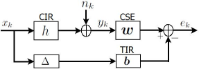
Figure 1: A schematic of the system model.

III Sparse Channel Shortening and Equalization

III-A Problem Formulation

As shown in Figure 1, in minimum-mean-square-error (MMSE) shortening [4], the objective is to design the CSE, $\boldsymbol{w}$, and the TIR, $\boldsymbol{b}$, filters such that the overall impulse response which is the convolution of the CIR and the CSE vectors best approximates, in the MSE sense, a TIR with few taps. We denote the span (the filter length) of the CSE by $N_{f}$ and the span of the TIR by $N_{b}$. The $k^{th}$ channel shortening error sample $e_{k}$ is defined as follows (see Figure 1):

$$e_{k} = \sum_{m=0}^{N_{f}-1}w_{n}^{*}\boldsymbol{y}_{k-m}-\sum_{n=0}^{N_{b}}b_{n}^{*}\boldsymbol{x}_{k-\Delta-n}$$ (8)

$$= \underbrace{\left[\begin{array}[]{cccc}w_{0}^{*}&w_{1}^{*}&\ldots&w_{N_{f}-1}^{*}\end{array}\right]}_{\boldsymbol{w}^{H}}\boldsymbol{y}_{k:k+N_{f}+1}-$$

$$\underbrace{\left[\begin{array}[]{cccccc}\boldsymbol{0}_{1\times\Delta}&b_{0}^{*}&b_{1}^{*}&\ldots&b_{N_{b}}^{*}&\boldsymbol{0}_{1\times s}\end{array}\right]}_{\boldsymbol{b}^{H}}\boldsymbol{x}_{k:k-N_{f}-v+1}$$

$$= \boldsymbol{w}^{H}\boldsymbol{y}_{k:k+N_{f}+1}-\boldsymbol{b}^{H}\boldsymbol{x}_{k:k-N_{f}-v+1}\,,$$ (9)

where $\Delta$ represents the decision delay and $s=N_{f}+v-\Delta-N_{b}-1$. Hence, the MSE, denoted as $\xi\left(\boldsymbol{w,b}\right)$ is given by

$$\!\!\!\!\!\!\!\xi\left(\boldsymbol{w,b}\right) \triangleq E\left[\left|e_{k}^{2}\right|\right]$$ (10)

$$= \!\!\boldsymbol{w}^{H}\boldsymbol{R}_{yy}\boldsymbol{w}-\boldsymbol{w}^{H}\boldsymbol{R}_{yx}\boldsymbol{b}-\boldsymbol{b}\boldsymbol{R}_{yx}^{H}\boldsymbol{w}^{H}+\boldsymbol{b}^{H}\boldsymbol{R}_{xx}\boldsymbol{b}.$$

Using the well-known orthogonality principle for MMSE, i.e., the error sequence is uncorrelated with the observed data, $E\left[e_{k}\boldsymbol{y}_{k:k+N_{f}+1}\right]=0$, we get

$$\boldsymbol{w}^{H}\boldsymbol{R}_{yy}=\boldsymbol{b}^{H}\boldsymbol{R}_{yx}.$$ (11)

Combining (10) and (11), we derive the MSE as

$$\xi\left(\boldsymbol{b}\right) = \boldsymbol{b}^{H}\underbrace{\left(\boldsymbol{R}_{xx}-\boldsymbol{R}_{xy}\boldsymbol{R}_{yy}^{-1}\boldsymbol{R}_{yx}\right)}_{\boldsymbol{R}_{\delta}}\boldsymbol{b}.$$ (12)

Minimizing $\xi\left(\boldsymbol{b}\right)$ over $\boldsymbol{b}$, gives the trivial solution $\boldsymbol{b}=0$. Thus, to preclude this trivial case, we minimize $\xi\left(\boldsymbol{b}\right)$ subject to the UTC where one of the $\left(N_{b}+1\right)$ nonzero taps is set to unity. The index of this unit tap $i$ $\left(0<i\leq N_{f}+v-1\right)$ is chosen such that the MSE $\xi\left(\boldsymbol{b}\right)$ is minimized. To minimize the MSE subject to the UTC, $\boldsymbol{b}^{H}\boldsymbol{e}_{i}=1$ (where $\boldsymbol{e}_{i}$ is the $i^{th}$ unit vector), we express $\boldsymbol{R}_{\delta}$ in (12) as $\boldsymbol{A}^{H}\boldsymbol{A}$ where $\boldsymbol{A}$ is the square root matrix of $\boldsymbol{R}_{\delta}$ in the spectral-norm sense, which results from Cholesky or eigen decomposition [14]. Then, (12) can be written as

$$\xi\left(\boldsymbol{b},i\right) = \boldsymbol{b}^{H}\boldsymbol{A}^{H}\boldsymbol{A}\boldsymbol{b}=\left\|\boldsymbol{A}\boldsymbol{b}\right\|_{2}^{2}$$ (13)

$$= \left\|\boldsymbol{\widetilde{A}}\,\widetilde{\boldsymbol{b}}+\boldsymbol{a}_{i}\right\|_{2}^{2}\,,$$

where $\boldsymbol{a}_{i}$ is the $i^{th}$ column of $\boldsymbol{A}$, $\boldsymbol{\widetilde{A}}$ is composed of all columns of $\boldsymbol{A}$ except $\boldsymbol{a}_{i}$, and $\widetilde{\boldsymbol{b}}$ is formed by all elements of $\boldsymbol{b}$ except the $i^{th}$ entry with unit value. Since only $\left(N_{b}+1\right)$ taps out of the total $\left(N_{f}+v\right)$ TIR taps are nonzero, the locations and weights of these taps need to be estimated such that $\xi\left(\boldsymbol{b}\right)$ is minimized. Towards this goal, we need first to optimize the location of the unit tap index $i$. By formulating the Lagrangian function: $\boldsymbol{\mathcal{L}}^{UTC}\left(\boldsymbol{b},\lambda\right)=\xi\left(\boldsymbol{b}\right)+\lambda\left(\boldsymbol{b}^{H}\boldsymbol{e}_{i}-1\right)$, where $\lambda$ is the Lagrangian multiplier, and then performing the minimization with respect to $\boldsymbol{b}$, we get [4]

$$\boldsymbol{b}_{opt}=\frac{\boldsymbol{R}_{\delta}^{-1}e_{i_{opt}}}{\boldsymbol{R}_{\delta}^{-1}\left(i_{opt},i_{opt}\right)}\,\,,\,\mbox{and}\,\,\,\,\,\mbox{MMSE}=\frac{1}{\boldsymbol{R}_{\delta}^{-1}\left(i_{opt},i_{opt}\right)}\,.$$ (14)

Note that $i_{opt}$ is the index that achieves the MMSE and is given by

$$i_{opt}\triangleq\underset{0<i\leq N_{f}+v-1}{\mbox{arg}\mbox{max}}\boldsymbol{R}_{\delta}^{-1}\left(i,i\right).$$ (15)

After computing $i_{opt}$, we formulate the following problem for the design of a sparse TIR filter:

$$\!\!\!\widetilde{\boldsymbol{b}}_{s} \triangleq \underset{\boldsymbol{b}\in\mathbb{C}^{N_{f}+v}}{\mbox{arg}\mbox{min}}\,\,\left\|\boldsymbol{b}\right\|_{0}\,\,\,\,\mbox{subject to}\,\,\,\,\,\xi\left(\boldsymbol{b},i_{opt}\right)\leq\delta_{cs}\,,$$ (16)

where $\left\|\boldsymbol{b}\right\|_{0}$ is the number of nonzero elements in its argument and the threshold $\delta_{cs}$ can be used as a design parameter to control the performance-complexity tradeoff. Although one can attempt to use convex-optimization-based approaches (after replacing $\left\|.\right\|_{0}$ with its convex approximation $\left\|.\right\|_{1}$ in (16) to reduce the search space [15]) for the sparse approximation vector, $\widetilde{\boldsymbol{b}}_{s}$, a number of greedy algorithms can be used to solve this problem efficiently with low complexity, especially in the situations where a specific number of $N_{b}$ taps is desired.

Once $\widetilde{\boldsymbol{b}}_{s}$ is calculated, we insert the unit tap in the $i^{th}$ location to construct the sparse TIR, $\boldsymbol{b}_{s}$. Then, the optimum CSE taps (in the MMSE sense) are determined from (11) to be

$$\boldsymbol{w}_{opt}=\boldsymbol{R}_{yy}^{-1}\overbrace{\boldsymbol{R}_{yx}\boldsymbol{b}_{s}}^{\boldsymbol{t}}.$$ (17)

Notice that the MMSE CSE, $\boldsymbol{w}_{opt}$, is not sparse and, hence, its design complexity still increases proportional to $(N_{f})^{2}$, which can be computationally expensive [16]. In contrast, any choice for $\boldsymbol{w}$ other than $\boldsymbol{w}_{opt}$ leads to performance loss, especially for channels with large delay spreads. Therefore, we also propose a sparse implementation for the FIR CSE, $\boldsymbol{w}$, as follows. After computing the TIR coefficients, $\boldsymbol{b}_{s}$, the MSE will be a function only of $\boldsymbol{w}$ and can be expressed as

$$\xi(\boldsymbol{w}) = \boldsymbol{w}^{H}\boldsymbol{R}_{yy}\boldsymbol{w}-\boldsymbol{w}^{H}\boldsymbol{R}_{yx}\boldsymbol{b}_{s}-\boldsymbol{b}_{s}\boldsymbol{R}_{yx}^{H}\boldsymbol{w}^{H}+\boldsymbol{b}_{s}^{H}\boldsymbol{R}_{xx}\boldsymbol{b}_{s}$$ (18)

$$= \!\underbrace{\boldsymbol{b}_{s}^{H}\boldsymbol{R}_{\delta}\boldsymbol{b}_{s}}_{\xi_{min}}+\underbrace{(\boldsymbol{w}-\boldsymbol{R}_{yy}^{-1}\boldsymbol{t})^{H}\boldsymbol{R}_{yy}(\boldsymbol{w}-\boldsymbol{R}_{yy}^{-1}\boldsymbol{t})}_{\xi_{ex}\left(\boldsymbol{w}\right)}\,.$$

The MSE $\xi\left(\boldsymbol{w}\right)$ is minimized by minimizing the term $\xi_{ex}(\boldsymbol{w})$ since $\xi_{min}$ does not depend on $\boldsymbol{w}$. Hence, the optimum choice for $\boldsymbol{w}$, in the MMSE sense, is the one given in (17). However, its computation and implementation complexity are high. Alternatively, to design a sprase CSE, we propose to use the excess MSE term, $\xi_{ex}\left(\boldsymbol{w}\right)$, as a design constraint to once again achieve a desirable performance-complexity tradeoff. In particular, we formulate the following problem for the design of sparse FIR CSE, $\boldsymbol{w}$:

$$\widehat{\boldsymbol{w}}_{s} \triangleq \underset{\boldsymbol{w}\in\mathbb{C}^{N_{f}}}{\mbox{arg}\mbox{min}}\,\,\left\|\boldsymbol{w}\right\|_{0}\,\,\,\,\mbox{subject to}\,\,\,\,\,\xi_{ex}\left(\boldsymbol{w}\right)\leq\delta_{eq}\,,$$ (19)

where $\delta_{eq}$ is a parameter selected by the designer to control the performance loss from the non-sparse highly-complex conventional CSE design based on the MMSE criterion. To solve (19), we can use either convex optimization or greedy algorithms with the latter being more desirable due to their low complexity. We are now ready to discuss a general framework for designing sparse CSE and TIR FIR filters such that the performance loss does not exceed an acceptable predefined limit.

III-B Proposed Sparse Approximation Framework

Unlike earlier works, including the one by one of the co-authors [10], we provide a general framework for designing both sparse CSE and TIR FIR filters that can be considered as the problem of sparse approximation using different dictionaries. Mathematically, this framework poses the design problem as follows:

$$\widehat{\boldsymbol{z}}_{s}\triangleq\underset{\boldsymbol{z}}{\mbox{\mbox{arg}\mbox{min}}}\,\left\|\boldsymbol{z}\right\|_{0}\,\,\,\mbox{subject to}\,\,\,\left\|\boldsymbol{K}\left(\boldsymbol{\varPhi}\boldsymbol{z}-\boldsymbol{d}\right)\right\|_{2}^{2}\leq\epsilon\,,$$ (20)

where $\boldsymbol{\varPhi}$ is the dictionary that will be used to sparsely approximate $\boldsymbol{d}$, while $\boldsymbol{K}$ is a known matrix and $\boldsymbol{d}$ is a known data vector, both of which change depending upon the sparsifying dictionary $\boldsymbol{\varPhi}$. Notice that $\widehat{\boldsymbol{z}}_{s}\in\left\{\widehat{\boldsymbol{w}}_{s},\,\widetilde{\boldsymbol{b}}_{s}\right\}$ and $\epsilon\in\left\{\delta_{cs},\,\delta_{eq}\right\}$. Notice that also by completing the square in (19) the problem reduces to the one shown in (20). Hence, one can use any factorization for $\boldsymbol{R}_{\delta}$ in (12) or $\boldsymbol{R}_{yy}$ in (18) to formulate a sparse approximation problem. Using the Cholesky or eigen decomposition for $\boldsymbol{R}_{\delta}$ or $\boldsymbol{R}_{yy}$, we will have different choices for $\boldsymbol{K}$, $\boldsymbol{\varPhi}$ and $\boldsymbol{d}$. For instance, by defining the Cholesky factorization [14] of $\boldsymbol{R}_{\delta}$ as $\boldsymbol{R}_{\delta}\triangleq\boldsymbol{L}_{\delta}\boldsymbol{L}_{\delta}^{H}$, or in the equivalent form $\boldsymbol{R}_{\delta}\triangleq\boldsymbol{P}_{\delta}\boldsymbol{\Sigma}_{\delta}\boldsymbol{P}_{\delta}^{H}=\boldsymbol{\varOmega}_{\delta}\boldsymbol{\varOmega}_{\delta}^{H}$ (where $\boldsymbol{L}_{\delta}$ is a lower-triangular matrix, $\boldsymbol{P}_{\delta}$ is a lower-unit-triangular (unitriangular) matrix and $\boldsymbol{\Sigma}_{\delta}$ is a diagonal matrix), the problem in (20) can, respectively, take one of the forms shown below:

$$\underset{\boldsymbol{b}\in\mathbb{C}^{N_{f}+v}}{\mbox{min}}\,\,\left\|\boldsymbol{b}\right\|_{0}\mbox{\,\,\,\,\mbox{s.t. }\,\,\,\,$\left\|\left(\widetilde{\boldsymbol{L}}_{\delta}^{H}\,\widetilde{\boldsymbol{b}}+\boldsymbol{l}_{i}\right)\right\|_{2}^{2}\leq\delta_{cs}\,$,}\,\mbox{and}$$ (21)

$$\underset{\boldsymbol{b}\in\mathbb{C}^{N_{f}+v}}{\mbox{min}}\,\,\left\|\boldsymbol{b}\right\|_{0}\mbox{\,\,\,\,\mbox{s.t. }\,\,\,\,$\left\|\left(\widetilde{\boldsymbol{\varOmega}}_{\delta}^{H}\,\widetilde{\boldsymbol{b}}+\boldsymbol{p}_{i}\right)\right\|_{2}^{2}\leq\delta_{cs}\,$.}$$ (22)

Recall that $\widetilde{\boldsymbol{\varOmega}}_{\delta}^{H}$ is formed by all columns of $\boldsymbol{\varOmega}_{\delta}^{H}$ except the $i^{th}$ column, $\boldsymbol{p}_{i}$ is the $i^{th}$ column of $\boldsymbol{\varOmega}_{\delta}^{H}$, and $\widetilde{\boldsymbol{b}}$ is formed by all entries of $\boldsymbol{b}$ except the $i^{th}$ unity entry. Similarly, by writing the Cholesky factorization of $\boldsymbol{R}_{yy}$ as $\boldsymbol{R}_{yy}\triangleq\boldsymbol{L}_{y}\boldsymbol{L}_{y}^{H}$ or the eigen decomposition of $\boldsymbol{R}_{yy}$ as $\boldsymbol{R}_{yy}\triangleq\boldsymbol{U}_{y}\boldsymbol{D}_{y}\boldsymbol{U}_{y}^{H}$, we can formulate the problem in (20) as follows:

$$\!\!\!\!\underset{\boldsymbol{w}\in\mathbb{C}^{N_{f}}}{\mbox{min}}\left\|\boldsymbol{w}\right\|_{0}\mbox{\,\,\,\,\mbox{s.t. }\,\,\,\,$\left\|\left(\boldsymbol{L}_{y}^{H}\boldsymbol{w}-\boldsymbol{L}_{y}^{-1}\boldsymbol{t}\right)\right\|_{2}^{2}\leq\delta_{eq}\,$,}$$ (23)

$$\!\!\!\!\!\!\!\!\!\!\!\,\underset{\boldsymbol{w}\in\mathbb{C}^{N_{f}}}{\mbox{min}}\left\|\boldsymbol{w}\right\|_{0}\mbox{\,\,\mbox{s.t. }\,\,$\left\|\left(\boldsymbol{D}_{y}^{\frac{1}{2}}\boldsymbol{U}_{y}^{H}\boldsymbol{w}-\boldsymbol{D}_{y}^{-\frac{1}{2}}\boldsymbol{U}_{y}^{H}\boldsymbol{t}\right)\right\|_{2}^{2}\leq\delta_{eq},\,\mbox{and}$}$$ (24)

$$\!\!\!\!\!\!\underset{\boldsymbol{w}\in\mathbb{C}^{N_{f}}}{\mbox{min}}\left\|\boldsymbol{w}\right\|_{0}\mbox{\,\,\,\,\mbox{s.t. }\,\,\,\,$\left\|\boldsymbol{L}_{y}^{-1}\left(\boldsymbol{R}_{yy}\boldsymbol{w}-\boldsymbol{t}\right)\right\|_{2}^{2}\leq\delta_{eq}$\,}.$$ (25)

Note that the sparsifying dictionaries in (23), (24) and (25) are $\boldsymbol{L}_{y}^{H}$, $\boldsymbol{D}_{y}^{\frac{1}{2}}\boldsymbol{U}_{y}^{H}$ and $\boldsymbol{R}_{yy}$, respectively. Furthermore, the matrix $\boldsymbol{K}$ is an identity matrix in all cases except in (25), where it is equal to $\boldsymbol{L}_{y}^{-1}$.

We conclude this section by pointing out that several other sparsifying dictionaries can be used to sparsely design the CSE and TIR FIR filters. Due to lack of space, we presented above some of those possible choices and the other choices can be derived by applying suitable transformations to (12) and (18).

III-C Reduced-Complexity Design

In this section, we propose reduced-complexity designs for the CSE and TIR FIR filters. The proposed designs in Section III-B involve Cholesky factorization and/or eigen decomposition, whose computational costs could be large for channels with large delay spreads. For a Toeplitz matrix, the most efficient algorithms for Cholesky factorization are Levinson or Schur algorithms [17], which involve $\mathcal{O}(M^{2})$ computations, where $M$ is the matrix dimension. In contrast, since a circulant matrix is asymptotically equivalent to a Toeplitz matrix, for reasonably large dimension [18], the eigen decomposition of a circulant matrix can be computed efficiently using the fast Fourier transform (FFT) and its inverse with only $\mathcal{O}\left(M\,\mbox{log}(M)\right)$ operations. By using this asymptotic equivalence between Toeplitz and circulant matrices, all computations needed for $\boldsymbol{R}_{yy}$ and $\boldsymbol{R}_{\delta}$ factorization can be done efficiently with the FFT and inverse FFT. In addition, direct matrix inversion can be avoided.

It is well known that a circulant matrix, $\boldsymbol{C}$, has the discrete Fourier transform (DFT) basis vectors as its eigenvectors and the DFT of its first column as its eigenvalues. An $M\times M$ circulant matrix $\boldsymbol{C}$ can be decomposed as $\boldsymbol{C}$ =$\frac{1}{M}\boldsymbol{F}_{M}^{H}\boldsymbol{\varLambda}_{\boldsymbol{c}}\boldsymbol{F}_{M}$, where $\boldsymbol{F}_{M}$ is the discrete Fourier transform (DFT) matrix with $f_{k,l}=e^{-j2\pi kl/M}$, $0\leq k,\,l\leq M-1$, and $\boldsymbol{\varLambda}_{\boldsymbol{c}}$ is an $M$ by $M$ diagonal matrix whose diagonal elements are the $M$-point DFT of $\boldsymbol{c}=\left\{c\right\}_{i=0}^{i=M-1}$, the first column of the circulant matrix. We denote by $\overline{\boldsymbol{R}}_{yy},\,\overline{\boldsymbol{R}}_{yx}$ and $\overline{\boldsymbol{R}}_{\delta}$ the circulant approximation to the matrices $\boldsymbol{R}_{yy},\,\boldsymbol{R}_{yx}\mbox{ and }\boldsymbol{R}_{\delta}$, respectively. In addition, we denote the noiseless channel output vector as $\widetilde{\boldsymbol{y}},$ i.e., $\widetilde{\boldsymbol{y}}=\boldsymbol{Hx}$. Hence, the autocorrelation matrix $\boldsymbol{\overline{R}}_{yy}$ is computed as

$$\boldsymbol{\overline{R}}_{yy}=\underbrace{E\left[\widetilde{\boldsymbol{y}}_{k}\widetilde{\boldsymbol{y}}_{k}\right]}_{\overline{\boldsymbol{R}}_{\widetilde{y}\widetilde{y}}}+\underbrace{\frac{1}{SNR}}_{\sigma_{n}^{2}}\boldsymbol{I}_{N_{f}}.$$ (26)

To approximate $\boldsymbol{R}_{yy}$ as a circulant matrix, we assume that $\left\{\widetilde{\boldsymbol{y}}_{k}\right\}$ is cyclic. Hence, $E\left[\widetilde{\boldsymbol{y}}_{k}\widetilde{\boldsymbol{y}}_{k}\right]$ can be approximated as a time-averaged autocorrelation function as follows:

$$\overline{\boldsymbol{R}}_{\widetilde{y}\widetilde{y}} = \frac{1}{N_{f}}\sum_{k=0}^{N_{f}-1}\widetilde{\boldsymbol{y}}_{k}\widetilde{\boldsymbol{y}}_{k}^{H}=\frac{1}{N_{f}}\boldsymbol{C}_{y}\boldsymbol{C}_{y}^{H}$$ (27)

$$= \frac{1}{N_{f}}\left(\frac{1}{N_{f}}\boldsymbol{F}_{N_{f}}^{H}\boldsymbol{\varLambda}_{\underline{\widetilde{\boldsymbol{Y}}}}\boldsymbol{F}_{N_{f}}\right)\left(\frac{1}{N_{f}}\boldsymbol{F}_{N_{f}}^{H}\boldsymbol{\varLambda}_{\underline{\widetilde{\boldsymbol{Y}}}}^{H}\boldsymbol{F}_{N_{f}}\right)$$

$$= \frac{1}{N_{f}^{2}}\boldsymbol{F}_{N_{f}}^{H}\boldsymbol{\varLambda}_{\underline{\widetilde{\boldsymbol{Y}}}}\varLambda_{\underline{\widetilde{\boldsymbol{Y}}}}^{H}\boldsymbol{F}_{N_{f}}$$

$$= \frac{1}{N_{f}^{2}}\left(\boldsymbol{F}_{N_{f}}^{H}\boldsymbol{\varLambda}_{\left|\underline{\widetilde{\boldsymbol{Y}}}\right|^{2}}\boldsymbol{F}_{N_{f}}\right)\,,$$

where $\underline{\widetilde{\boldsymbol{Y}}}$ is the $N_{f}$-point DFT of $\boldsymbol{c}_{1}=\left[\begin{array}[]{cccc}\widetilde{y}_{N_{f}-1}&\widetilde{y}_{N_{f}-2}&\ldots&\widetilde{y}_{0}\end{array}\right]$, $\boldsymbol{F}_{N_{f}}$ is an $N_{f}\times N_{f}$ DFT matrix. $\left|.\right|$ denotes element-wise norm square, and $\boldsymbol{C}_{y}=\mbox{{circ}}\left(\boldsymbol{c}_{1}\right)$ where circ denotes a circulant matrix whose first column is $\boldsymbol{c}_{1}$. Note that $\boldsymbol{F}_{N_{f}}^{H}\boldsymbol{F}_{N_{f}}=\boldsymbol{F}_{N_{f}}\boldsymbol{F}_{N_{f}}^{H}=N_{f}\boldsymbol{I}_{N_{f}}$.

Without loss of generality, we can write the noiseless channel output sequence $\widetilde{\boldsymbol{y}}_{k}$ in the discrete frequency domain as a column vector form as

$$\widetilde{\boldsymbol{\underline{Y}}} = \boldsymbol{\underline{H}}^{H}\odot\boldsymbol{\underline{P}}_{\Delta}\odot\boldsymbol{\underline{X}}\,,$$ (28)

where $\boldsymbol{\underline{H}}$ is the $N_{f}$-point DFT of the CIR $\boldsymbol{h}$, $\boldsymbol{\underline{P}}_{\Delta}=\left[\begin{array}[]{cccc}1&e^{-j2\pi\Delta/N_{f}}&\ldots&e^{-j2\pi\left(N_{f}-1\right)\Delta/N_{f}}\end{array}\right]^{T}$, and $\odot$ denotes element-wise multiplication. Note that $\left|\widetilde{\boldsymbol{\underline{Y}}}\right|^{2}=N_{f}\left|\boldsymbol{\underline{H}}\right|^{2}$. Then,

$$\boldsymbol{\overline{R}}_{yy} = \overline{\boldsymbol{R}}_{\widetilde{y}\widetilde{y}}+\sigma_{n}^{2}\boldsymbol{I}_{N_{f}}$$ (29)

$$= \frac{1}{N_{f}^{2}}\boldsymbol{F}_{N_{f}}^{H}\left(\boldsymbol{\varLambda}_{N_{f}\left|\boldsymbol{\underline{H}}\right|^{2}+N_{f}\sigma_{n}^{2}\boldsymbol{1}_{N_{f}}}\right)\boldsymbol{F}_{N_{f}}$$

$$= \boldsymbol{F}_{N_{f}}^{H}\left(\frac{1}{N_{f}}\boldsymbol{\varLambda}_{\underbrace{\left|\underline{\boldsymbol{H}}\right|^{2}+\sigma_{n}^{2}\boldsymbol{1}_{N_{f}}}_{\varrho}}\right)\boldsymbol{F}_{N_{f}}$$

$$= \boldsymbol{F}_{N_{f}}^{H}\left(\frac{1}{N_{f}}\boldsymbol{\varLambda}_{\varrho}\right)\boldsymbol{F}_{N_{f}}=\boldsymbol{Q}\boldsymbol{Q}^{H}.$$

Using the matrix inversion lemma [14], the inverse of $\boldsymbol{\overline{R}}_{yy}$ is then

$$\boldsymbol{\overline{R}}_{yy}^{-1} \!\!\!\!= \!\!\!\left\{\boldsymbol{F}_{N_{f}}^{H}\left(\frac{1}{N_{f}}\boldsymbol{\varLambda}_{\varrho}\right)\boldsymbol{F}_{N_{f}}\right\}^{-1}$$ (30)

$$\!\!\!\!\!= \!\!\!\!\boldsymbol{F}_{N_{f}}^{H}\!\left[\!\frac{1}{N_{f}\sigma_{n}^{2}}\!\left(\!\boldsymbol{I}_{N_{f}}-\frac{1}{N_{f}\sigma_{n}^{2}}\boldsymbol{\varLambda}_{\underline{\widetilde{\boldsymbol{Y}}}}\!\left(\!\boldsymbol{\varLambda}_{\underline{\widetilde{\boldsymbol{Y}}}}^{H}\varLambda_{\underline{\widetilde{\boldsymbol{Y}}}}+\boldsymbol{I}_{N_{f}}\!\right)^{-1}\!\!\boldsymbol{F}_{N_{f}}\!\right)\!\right]$$

$$\!\!\!\!= \!\!\!\frac{1}{N_{f}\sigma_{n}^{2}}\boldsymbol{F}_{N_{f}}^{H}\left(\boldsymbol{I}_{N_{f}}-\frac{1}{N_{f}}\boldsymbol{\varLambda}_{\underline{\widetilde{\boldsymbol{Y}}}}\boldsymbol{\varLambda}_{\varrho}^{-1}\boldsymbol{\varLambda}_{\underline{\widetilde{\boldsymbol{Y}}}}^{H}\right)\boldsymbol{F}_{N_{f}}.$$

Similarly, $\boldsymbol{R}_{\delta}$ can be expressed as

$$\overline{\boldsymbol{R}}_{\delta} = \boldsymbol{R}_{xx}-\boldsymbol{\overline{R}}_{yx}^{H}\boldsymbol{\overline{R}}_{yy}^{-1}\boldsymbol{\overline{R}}_{yx}$$ (31)

$$= \boldsymbol{R}_{xx}-\boldsymbol{\overline{R}}_{yx}^{H}\boldsymbol{\overline{R}}_{yy}^{-1}\left\{\frac{1}{N^{2}}\widetilde{\boldsymbol{F}}_{N_{f}}^{H}\left(\boldsymbol{\varLambda}_{\underline{\widetilde{\boldsymbol{Y}}}}\boldsymbol{\varLambda}_{\boldsymbol{\underline{X}}}^{H}\right)\boldsymbol{F}_{N}\right\}$$

$$= \boldsymbol{I}_{N}-\boldsymbol{\overline{R}}_{yx}^{H}\times$$

$$\left\{\frac{1}{N^{2}\sigma_{n}^{2}}\widetilde{\boldsymbol{F}}_{N_{f}}^{H}\left(\boldsymbol{\varLambda}_{\underline{\boldsymbol{Y}}}\boldsymbol{\varLambda}_{\boldsymbol{\underline{X}}}^{H}-\boldsymbol{\varLambda}_{\boldsymbol{\underline{Y}}}\boldsymbol{\varLambda}_{\overline{\theta}\varoslash\theta}\boldsymbol{\varLambda}_{\boldsymbol{\underline{X}}}^{H}\right)\boldsymbol{F}_{N}\right\}$$

$$= \boldsymbol{I}_{N}-\boldsymbol{\overline{R}}_{xy}\left\{\frac{1}{N\sigma_{n}^{2}}\boldsymbol{F}_{N}^{H}\left(\boldsymbol{\varLambda}_{\underline{\widetilde{\boldsymbol{Y}}}}\boldsymbol{\varLambda}_{1\varoslash\theta}\boldsymbol{\varLambda}_{\underline{\widetilde{\boldsymbol{Y}}}}^{H}\right)\boldsymbol{F}_{N}\right\}$$

$$= \boldsymbol{I}_{N}-\left\{\frac{1}{N^{2}}\boldsymbol{F}_{N}^{H}\left(\boldsymbol{\varLambda}_{\boldsymbol{\underline{X}}}\boldsymbol{\varLambda}_{\underline{\widetilde{\boldsymbol{Y}}}}^{H}\boldsymbol{\varLambda}_{\underline{\widetilde{\boldsymbol{Y}}}}\boldsymbol{\varLambda}_{1\varoslash\theta}\boldsymbol{\varLambda}_{\boldsymbol{\underline{X}}}^{H}\right)\boldsymbol{F}_{N}\right\}$$

$$= \frac{1}{N^{2}}\boldsymbol{F}_{N}^{H}\left(N\,\boldsymbol{I}_{N}-\boldsymbol{\varLambda}_{\boldsymbol{\underline{X}}}\boldsymbol{\varLambda}_{\overline{\theta}\varoslash\theta}\boldsymbol{\varLambda}_{\boldsymbol{\underline{X}}}^{H}\right)\boldsymbol{F}_{N}$$

$$= \frac{1}{N}\boldsymbol{F}_{N}^{H}\left(\boldsymbol{I}_{N}-\boldsymbol{\varLambda}_{\overline{\theta}\varoslash\theta}\right)\boldsymbol{F}_{N}$$

$$= \boldsymbol{\varGamma}\boldsymbol{\varGamma}^{H},$$

where $\varoslash$ denotes element-wise division, $N=N_{f}+v$, $\widetilde{\boldsymbol{F}}_{N_{f}}^{H}$ is an $N\times N_{f}$ DFT matrix, $\theta=\overline{\theta}+N\sigma_{n}^{2}\boldsymbol{1}_{N}$, and $\overline{\theta}=\left|\widetilde{\boldsymbol{\underline{Y}}}\right|^{2}$. Substituting (29) and (31) into (18) and (12), respectively, we can design the CSE and TIR FIR filters in a reduced-complexity manner where neither a Choleskey nor an eigen factorization is needed.

We have now shown that the problem of designing sparse CSE and TIR FIR filters can be cast into one of sparse approximation of a vector by a fixed dictionary. Furthermore, this dictionary can be obtained in an efficient manner using only the FFT and its inverse. The general form of this problem is given by (20). To solve this problem, we use the well-known Orthogonal Matching Pursuit (OMP) greedy algorithm [19] that estimates $\widehat{\boldsymbol{z}}_{s}$ by iteratively selecting a set $S$ of the sparsifying dictionary columns (i.e., atoms $\boldsymbol{\phi}_{i}$’s) of $\boldsymbol{\varPhi}$ that are most correlated with the data vector $\boldsymbol{d}$ and then solving a restricted least-squares problem using the selected atoms. The OMP stopping criterion ($\rho$) is traditionally either a predefined sparsity level (number of nonzero entries) of $\boldsymbol{z_{s}}$ or an upper-bound on the norm of the residual error. In our problem, $\rho$ in the latter case is changed from an upper-bound on the residual error norm to an upper-bound on the norm of the Projected Residual Error (PRE), i.e., “$\boldsymbol{K}\times\mbox{Residual Error}$”. The computations involved in the OMP algorithm are well documented in the sparse approximation literature (e.g., [19]) and are omitted here due to page limitations.

Note that unlike conventional compressive sensing techniques [20], where the measurement matrix is a fat matrix, the sparsifying dictionary in our framework is either a tall matrix (fewer columns than rows) with full column rank as in (21) and (22) or a square one with full rank as in (23)–(25). However, OMP and similar methods can still be used if $\boldsymbol{R}_{yy}$ and $\boldsymbol{R}_{\delta}$ can be decomposed into $\boldsymbol{\Psi}\boldsymbol{\Psi}^{H}$ and the data vector $\boldsymbol{d}$ is compressible [21, 22].

Our next challenge is to determine the best sparsifying dictionary for use in our framework. We know from the sparse approximation literature that the sparsity of the OMP solution tends to be inversely proportional to the worst-case coherence $\mu\left(\boldsymbol{\varPhi}\right)$, $\mu\left(\boldsymbol{\varPhi}\right)\triangleq\underset{i\neq j}{\mbox{max}}\frac{\left|\left\langle\phi_{i},\,\phi_{j}\right\rangle\right|\,}{\left\|\phi_{i}\right\|_{2}\left\|\phi_{j}\right\|_{2}}$ [23, 24]. Notice that $\mu\left(\boldsymbol{\varPhi}\right)\in\left[0,1\right]$. Next, we investigate the coherence of the dictionaries involved in our analysis.

III-D Worst-Case Coherence Analysis

We perform a coherence metric analysis to gain some insight into the performance of the proposed sparsifying dictionaries and the behavior of the resulting sparse CSE and TIR FIR filters. First and foremost, we are concerned with analyzing $\mu\left(\boldsymbol{\varPhi}\right)$ to ensure that it does not approach $1$ for any of the proposed sparsifying dictionaries. In addition, we are interested in identifying which $\boldsymbol{\varPhi}$ has the smallest coherence and, hence, gives the sparsest design. We have two kinds of sparsifying dictionaries. The first kind is the dictionaries resulting from $\boldsymbol{R}_{\delta}$ factorization while the second kind is either $\boldsymbol{R}_{yy}$ itself or any of its factors. We proceed as follows to characterize upper-bounds on each kind of dictionary. We estimate upper bounds on the worst-case coherence of both $\boldsymbol{R}_{\delta}$ and $\boldsymbol{R}_{yy}$ separately and evaluate their closeness to $1$. Then, through simulation, we demonstrate that the coherence of the $\boldsymbol{R}_{\delta}$ and $\boldsymbol{R}_{yy}$ factors will be less than that of $\mu(\boldsymbol{R}_{\delta})$ and $\mu(\boldsymbol{R}_{yy})$, respectively. It is important to note here that the other dictionaries, which result from decomposing $\boldsymbol{R}_{\delta}$ and $\boldsymbol{R}_{yy}$, can be considered as square roots of them in the spectral-norm sense. For example, $\left\|\boldsymbol{R}_{yy}\vphantom{\boldsymbol{L}^{H}}\right\|_{2}=\left\|\boldsymbol{L}_{y}\boldsymbol{L}_{y}^{H}\right\|_{2}\leq\left\|\boldsymbol{L}_{y}^{H}\boldsymbol{\vphantom{\boldsymbol{L}^{H}}}\right\|_{2}^{2}$ and $\left\|\boldsymbol{R}_{\delta}\vphantom{\boldsymbol{\boldsymbol{U}}_{\delta}^{H}}\right\|_{2}=\left\|\boldsymbol{\boldsymbol{U}}_{\delta}\boldsymbol{D}_{\delta}\boldsymbol{\boldsymbol{U}}_{\delta}^{H}\right\|_{2}\leq\left\|\boldsymbol{D}_{\delta}^{1/2}\boldsymbol{\boldsymbol{U}}_{\delta}^{H}\right\|_{2}^{2}$.

Even though the matrix $\boldsymbol{R}_{\delta}$ is comprised of Toeplitz matrices, it is generally non-Toeplitz. We use its factors in our framework to compute $\widetilde{\boldsymbol{b}}$ that best approximates $\boldsymbol{\widetilde{A}}\,\widetilde{\boldsymbol{b}}$ to $\boldsymbol{a}_{i}$ as shown in (13). The formula of $\boldsymbol{R}_{\delta}$ in (12) can be written in terms of the SNR and CIR coefficients as $\boldsymbol{R}_{\delta}=\left[\boldsymbol{R}_{xx}^{-1}+\boldsymbol{H}^{H}\boldsymbol{R}_{nn}^{-1}\boldsymbol{H}\right]^{-1}=\left[\boldsymbol{I}+\frac{1}{\sigma_{n}^{2}}\boldsymbol{H}^{H}\boldsymbol{H}\right]^{-1}$. Hence, at low SNR, the noise effect dominates, i.e., $\boldsymbol{R}_{\delta}\approx\boldsymbol{I}$, and, consequently, $\mu\left(\boldsymbol{R}_{\delta}\right)\rightarrow 0$. As the SNR increases, the noise effect decreases and the effect of the channel taps starts to appear which makes $\mu\left(\boldsymbol{R}_{\delta}\right)$ converge to a constant. Through simulation, we show that this constant does not approach $1$ and, accordingly, the other dictionaries generated from $\boldsymbol{R}_{\delta}$ have a coherence that is also less than that of $\mu\left(\boldsymbol{R}_{\delta}\right)$.

On the other hand, $\boldsymbol{R}_{yy}$ has a well-structured (Hermitian Toeplitz) closed-form in terms of the CIR coefficients, filter time span $N_{f}$ and SNR, i.e., $\boldsymbol{R}_{yy}=\boldsymbol{H}\boldsymbol{H}^{H}+\mbox{$\frac{\mbox{1}}{SNR}$}\boldsymbol{I}$. It can be expressed in matrix form as

$$\boldsymbol{R}_{yy}=\mbox{Toeplitz}\overbrace{\left(\left[\begin{array}[]{ccccccc}r_{0}&r_{1}&\ldots&r_{v}&0&\ldots&0\end{array}\right]\right)}^{\boldsymbol{\phi}_{1}^{H}}\,,$$ (32)

where $r_{0}={\displaystyle\sum_{i=0}^{v}\left|h_{i}\right|^{2}+\left(\mbox{SNR}\right)^{-1}}$, $r_{j}=\sum_{i=j}^{v}h_{i}h_{i-j}^{*},\,\forall j\neq 0$. In [11], we showed that an upper-bound on $\mu(\boldsymbol{R}_{yy})$ in the high SNR setting can be derived by solving the following optimization problem

$$\underset{\boldsymbol{h}}{\mbox{\mbox{max}}}\,\,\,\left|\boldsymbol{h}^{H}\boldsymbol{R}\boldsymbol{h}\right|\,\,\,\,\,\,\,\mbox{s.t.}\,\,\,\,\,\,\,\boldsymbol{h}^{H}\boldsymbol{h}=1\,,$$ (33)

where $\boldsymbol{h}=\left[\begin{array}[]{cccc}h_{0}&h_{1}&\ldots&h_{v}\end{array}\right]^{H}$ is the length-$(v+1)$ CIR vector and $\boldsymbol{R}$ is a matrix that has ones along the super and sub-diagonals. It is also shown that the solution of (33) is the eigenvector corresponding to the maximum eigenvalue of $\boldsymbol{R}$. The eigenvalues $\lambda_{s}$ and eigenvectors $h_{j}^{(s)}$ of the matrix $\boldsymbol{R}$ have the following simple closed-forms [25]:

$$\lambda_{s} = 2\,\mbox{cos}(\frac{\pi s}{v+2})\,\,\,\,,\,\,\,\,h_{j}^{(s)}=\sqrt{\frac{2}{v+2}}\mbox{sin$(\frac{j\pi s}{v+2})\,,\,$}$$ (34)

where $s,j=1,\ldots,v+1.$ Finally, by numerically evaluating $h_{j}^{(s)}$ for the maximum $\lambda_{s}$, we find that the worst-case coherence of $\boldsymbol{R}_{yy}$ (for any $v$) is sufficiently less than 1. This observation points to the likely success of OMP in providing the sparsest solution $\widehat{\boldsymbol{w}}_{s}$ which corresponds to the dictionary that has the smallest coherence. Next, we will report the results of our numerical experiments to evaluate the performance of our proposed framework under different sparsifying dictionaries.

IV Simulation Results

The CIRs used in our numerical results are unit-energy symbol-spaced FIR filters with $v$ taps generated as zero-mean uncorrelated complex Gaussian random variables. The CIR taps are assumed to have a uniform power-delay-profile (UPDP). The performance results are calculated by averaging over 5000 channel realizations. We use the notation $\boldsymbol{D}(\boldsymbol{\chi}_{t},\,\boldsymbol{\chi}_{e})$ to refer to a TIR designed based on the sparsifying dictionary $\boldsymbol{\chi}_{t}$ and a CSE designed based on the sparsifying dictionary $\boldsymbol{\chi}_{e}$.

To quantify the accuracy of approximating the matrices $\boldsymbol{R}_{yy},\,\boldsymbol{R}_{\delta}$ by their equivalent circulant matrices $\boldsymbol{\overline{R}}_{yy}$ and $\overline{\boldsymbol{R}}_{\delta}$, respectively, we plot the optimal shortening SNR and the shortening SNR obtained from the circulant approximation versus the number of CSE taps ($N_{f}$) in Figure 2. The gap between the optimal shortening SNR and the shortening SNR from the circulant approximation approaches zero as the number of the CSE taps increases, as expected. A good choice for $N_{f}$, to obtain an accurate approximation, would be $N_{f}\geq 5v$.

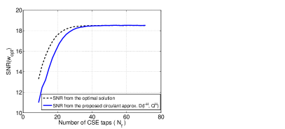
Figure 2: Performance of circulant approximation based approach for UPDP channel with $v=5$ and input $\mbox{SNR}=20\,\mbox{dB}$.

   

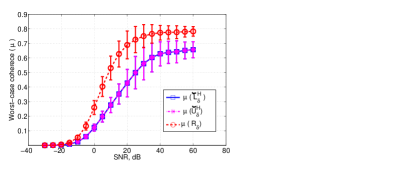
Figure 3: Worst-case coherence for the sparsifying dictionaries $\widetilde{\boldsymbol{L}}_{\delta}$ and $\widetilde{\boldsymbol{U}}_{\delta}$ versus input SNR for UPDP with $v=8$ and $N_{f}=80$. Note that we estimate $\mu(\boldsymbol{\varPhi})$ after removing the column corresponding to the $i^{th}$ unit tap as discussed in (13). Moreover, changing the location of the $i^{th}$ column has insignificant effect on $\mu(\boldsymbol{\varPhi})$.

      

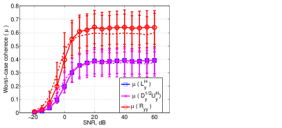
Figure 4: Worst-case coherence for the sparsifying dictionaries $\boldsymbol{L}_{y}^{H}$, $\boldsymbol{D}_{y}^{\frac{1}{2}}\boldsymbol{U}_{y}^{H}$ and $\boldsymbol{R}_{yy}$ versus input SNR for UPDP with $v=8$ and $N_{f}=80$. Dashed lines represent the coherence of the corresponding circulant approximation for $\boldsymbol{D}_{y}^{\frac{1}{2}}\boldsymbol{U}_{y}^{H}$ (i.e., $\boldsymbol{Q}^{H}$) and $\boldsymbol{R}_{yy}$ (i.e., $\boldsymbol{\overline{R}}_{yy}=$$\boldsymbol{Q}$$\boldsymbol{Q}^{H}$).

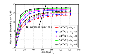
Figure 5: Maximum shortening SNR versus CSE taps for UPDP CIR with $v=5$, SNR = $20$ dB. Solid lines represent the $\boldsymbol{D}(\boldsymbol{\varGamma}^{H},\boldsymbol{Q}^{H})$ approach while the dashed lines represent the “significant-taps” approach proposed in [12].

To investigate the performance of the sparsifying dictionaries used in our analysis in terms of coherence, we plot the worst-case coherence versus the input SNR in Figure 3 for sparsifying dictionaries $\widetilde{\boldsymbol{L}}_{\delta}$ and $\widetilde{\boldsymbol{U}}_{\delta}$ (which is formed by all columns of $\boldsymbol{D}_{\delta}^{\frac{1}{2}}\boldsymbol{U}_{\delta}^{H}$ except the $i^{th}$ column) generated from $\boldsymbol{R}_{\delta}$. Note that a smaller value of $\mu(\boldsymbol{\Phi})$ indicates that a reliable sparse approximation is more likely. Both sparsifying dictionaries have the same $\mu\left(\boldsymbol{\varPhi}\right)$, which is strictly less than $1$. Similarly, in Figure 4, we plot the worst-case coherence of the proposed sparsifying dictionaries which we used to design the sparse CSE. At high SNR levels, the noise effects are negligible and, hence, the sparsifying dictionaries (e.g., $\boldsymbol{R}_{yy}\approx\boldsymbol{H}\boldsymbol{H}^{H}$) do not depend on the SNR. As a result, the coherence converges to a constant. On the contrary, at low SNR, the noise effects dominate the channel effects. Hence, the channel can be approximated as a memoryless (i.e., 1 tap) channel. As such the dictionaries (e.g., $\boldsymbol{R}_{yy}\approx\frac{1}{SNR}\boldsymbol{I}$) can be approximated as a multiple of the identity matrix, i.e., $\mu\left(\boldsymbol{\varPhi}\right)\rightarrow 0$.

In Figure 5, we compare our proposed sparse TIR design with that in [12], which we refer to it as the “significant-taps” approach, in terms of shortening SNR where we plot the shortening SNR versus CSE taps $N_{f}$ for the UPDP channel. We vary $N_{b}$, the number of TIR taps, from $1$ (lower curve) to $5$ (upper curve). The shortening SNR increases as $N_{b}$ increases for all TIR designs, as expected, and our sparse TIR outperforms, for all scenarios, the proposed approach in [12]. Notice that as $N_{b}$ increases, the sparse TIR becomes more accurate in approximating the actual CIR.

Next, we compare the sparse TIR designs to study the effect of $\mu\left(\boldsymbol{\varPhi}\right)$ on their performance. The OMP algorithm is used to compute the sparse approximations. The OMP stopping criterion is set to be either a predefined number of nonzero taps $N_{b}$ or a function of the PRE such that: Performance Loss ($\eta$)$=10\,\mbox{Log}_{10}\left(\frac{SNR(\boldsymbol{w}_{s})}{SNR(\boldsymbol{w}_{opt})}\right)\leq 10\,\mbox{Log}_{10}\left(1+\frac{{}_{\delta_{eq}}}{\xi_{m}}\right)\triangleq\eta_{max}$. Here, $\delta_{eq}$ is computed based on an acceptable $\eta_{max}$ and, then, the coefficients of $\widehat{\boldsymbol{w}}_{s}$ are computed using (20). The percentage of the active taps is calculated as the ratio between the number of nonzero taps to the total number of filter taps, i.e., $N_{f}$. For the optimal CSE, where none of the coefficients is zero, the number of active filter taps is equal to the filter span. The decision delay $\Delta$ and the unit-tap index $i$ should be optimized to avoid performance degradation. However, a near optimum performance is achieved by choosing these parameters to be around $(N_{f}+v)/2$ [4].

          

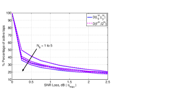
Figure 6: Percentage of active CSE taps versus the performance loss ($\eta_{max}$) for sparse TIR designs with SNR = 20 dB, $v=5$ and $N_{f}=40$.

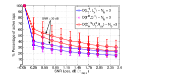
Figure 7: Percentage of active CSE taps versus the performance loss ($\eta_{max}$) for a sparse TIR with $N_{b}=3$, SNR = 20 dB, 30 dB, $v=8$ and $N_{f}=80$.

The effect of our sparse CSE and TIR FIR filter designs on the performance is shown in Figure 6. We plot the number of active (non-zero) CSE taps as a percentage of the total CSE span $N_{f}$ versus the maximum loss in the shortening SNR. Allowing a higher loss in the shortening SNR yields a bigger reduction in the number of CSE taps. Moreover, the active CSE taps percentage increases as $N_{b}$ decreases because the equalizer needs more taps to shorten the CIR to a shorter TIR. We also observe that allowing a maximum of only 0.25 dB in SNR loss with $N_{b}=2$ results in a substantial $60\%$ reduction in the number of CSE active taps (the equalizer can shorten the channel using only 16 out of 40 taps).

In Figure 7, we plot the percentage of the active CSE taps versus $\eta_{max}$ for different sparsifying dictionaries assuming $N_{b}=3$. We notice that a lower active taps percentage is obtained when the coherence of the sparsifying dictionary is smaller. For instance, allowing for $0.25$ dB SNR loss results in a significant reduction in the number of active CSE taps. Almost $60\%$ of the taps are eliminated when using $\boldsymbol{D}(\boldsymbol{\varGamma}^{H},\boldsymbol{Q}^{H})$ and $\boldsymbol{D}(\boldsymbol{L}_{\delta}^{H},\,\boldsymbol{L}_{y}^{H})$ at SNR equals to 30 dB. $\boldsymbol{D}(\boldsymbol{D}_{\delta}^{\frac{1}{2}}\boldsymbol{U}_{\delta}^{H},\,\boldsymbol{R}_{yy})$ needs more active taps to achieve the same SNR loss as that of the other dictionaries due to its higher coherence for a given constraint on TIR taps $N_{b}$. This suggests that the smaller the worst-case coherence is, the sparser the CSE will be. Moreover, a lower sparsity level (active taps percentage) is achieved at higher SNR levels which is consistent with the previous findings (e.g., in [28]). Moreover, reducing the number of active taps decreases the design complexity and, consequently, the power consumption since a smaller number of complex multiply-and-add operations are required.

V Conclusions

In this paper, we proposed a general framework for sparse CSE and TIR FIR designs based on a sparse approximation formulation using different dictionaries. Based on the asymptotic equivalence of Toeplitz and circulant matrices, we proposed reduced-complexity designs, for both CSE and TIR FIR filters, where matrix factorizations can be carried out efficiently using the FFT and inverse FFT with negligible performance loss as the number of filter taps increases. In addition, we analyzed the coherence of the proposed dictionaries involved in our design and showed that the dictionary with the smallest coherence gives the sparsest filter design. The significance of our approach was also quantified through simulations.

References

• [1] J.ย A. Bingham, โ€œMulticarrier modulation for data transmission: An idea whose time has come,โ€ IEEE Commun. Magazine, vol.ย 28, no.ย 5, pp. 5โ€“14, 1990.
• [2] N.ย C. McGinty, R.ย A. Kennedy, and P.ย Hoeher, โ€œParallel trellis Viterbi algorithm for sparse channels,โ€ IEEE Commun. Letters, vol.ย 2, no.ย 5, pp. 143โ€“145, 1998.
• [3] A.ย M. Tonello, S.ย Dโ€™Alessandro, and L.ย Lampe, โ€œCyclic prefix design and allocation in bit-loaded OFDM over power line communication channels,โ€ IEEE Trans. on Commun., vol.ย 58, no.ย 11, pp. 3265โ€“3276, 2010.
• [4] N.ย Al-Dhahir and J.ย M. Cioffi, โ€œEfficiently computed reduced-parameter input-aided MMSE equalizers for ML detection: A unified approach,โ€ IEEE Trans. on Info. Theory, vol.ย 42, no.ย 3, pp. 903โ€“915, 1996.
• [5] N.ย Al-Dhahir, โ€œFIR channel-shortening equalizers for MIMO ISI channels,โ€ IEEE Trans. on Commun., vol.ย 49, no.ย 2, pp. 213โ€“218, 2001.
• [6] P.ย Melsa, R.ย Younce, and C.ย Rohrs, โ€œImpulse response shortening for discrete multitone transceivers,โ€ IEEE Trans. on Commun., vol.ย 44, no.ย 12, pp. 1662โ€“1672, Dec 1996.
• [7] D.ย Falconer and F.ย Magee, โ€œAdaptive channel memory truncation for maximum likelihood sequence estimation,โ€ Bell System Technical Journal, vol.ย 52, no.ย 9, pp. 1541โ€“1562, 1973.
• [8] A.ย Chopra and B.ย L. Evans, โ€œDesign of sparse filters for channel shortening,โ€ Journal of Signal Processing Systems, vol.ย 66, no.ย 3, pp. 259โ€“272, 2012.
• [9] J.ย Balakrishnan, R.ย K. Martin, and C.ย R. Johnsonย Jr, โ€œBlind, adaptive channel shortening by sum-squared auto-correlation minimization (SAM),โ€ IEEE Trans. on Sig. Processing, vol.ย 51, no.ย 12, pp. 3086โ€“3093, 2003.
• [10] A.ย Gomaa and N.ย Al-Dhahir, โ€œA new design framework for sparse FIR MIMO equalizers,โ€ IEEE Trans. on Commun., vol.ย 59, no.ย 8, pp. 2132โ€“2140, 2011.
• [11] A.ย O. Al-Abbasi, R.ย Hamila, W.ย U. Bajwa, and N.ย Al-Dhahir, โ€œA General Framework for the Design and Analysis of Sparse FIR Linear Equalizers.โ€ย ย ย in IEEE GlobalSIP Conference, 2015, pp. 1โ€“5.
• [12] S.ย Roy, T.ย M. Duman, and V.ย K. McDonald, โ€œError rate improvement in underwater MIMO communications using sparse partial response equalization,โ€ IEEE Journal of Oceanic Engineering, vol.ย 34, no.ย 2, pp. 181โ€“201, 2009.
• [13] S.ย Haykin, Adaptive Filter Theory (3rd Ed.).ย ย ย Upper Saddle River, NJ, USA: Prentice-Hall, Inc., 1996.
• [14] R.ย A. Horn and C.ย R. Johnson, Eds., Matrix Analysis.ย ย ย New York, NY, USA: Cambridge University Press, 1986.
• [15] J.ย A. Tropp, โ€œJust relax: Convex programming methods for identifying sparse signals in noise,โ€ IEEE Trans. on Info. Theory, vol.ย 52, no.ย 3, pp. 1030โ€“1051, 2006.
• [16] J.ย Proakis and M.ย Salehi, Digital Communications, 5th Edition.ย ย ย New York, NY, USA: McGraw-Hill, 2007.
• [17] M.ย H. Hayes, Statistical Digital Signal Processing and Modeling, 1stย ed.ย ย ย New York, NY, USA: John Wiley & Sons, Inc., 1996.
• [18] J.ย Pearl, โ€œOn coding and filtering stationary signals by discrete Fourier transforms (Corresp.),โ€ IEEE Trans. on Info. Theory, vol.ย 19, no.ย 2, pp. 229โ€“232, 1973.
• [19] J.ย Tropp and A.ย Gilbert, โ€œSignal recovery from random measurements via orthogonal matching pursuit,โ€ IEEE Trans. on Info. Theory, vol.ย 53, no.ย 12, pp. 4655โ€“4666, 2007.
• [20] D.ย L. Donoho, โ€œCompressed sensing,โ€ IEEE Trans. on Info. Theory, vol.ย 52, no.ย 4, pp. 1289โ€“1306, 2006.
• [21] X.ย Feng, โ€œSparse equalizer filter design for multi-path channels,โ€ Masterโ€™s thesis, Massachusetts Institute of Technology, 2012.
• [22] D.ย Wei, C.ย Sestok, and A.ย Oppenheim, โ€œSparse filter design under a quadratic constraint: Low-complexity algorithms,โ€ IEEE Trans. on Sig. Processing, vol.ย 61, no.ย 4, pp. 857โ€“870, 2013.
• [23] W.ย U. Bajwa and A.ย Pezeshki, โ€œFinite frames for sparse signal processing,โ€ in Finite Frames.ย ย ย Springer, 2013.
• [24] J.ย Tropp, โ€œGreed is good: algorithmic results for sparse approximation,โ€ IEEE Trans. on Info. Theory,, vol.ย 50, no.ย 10, pp. 2231โ€“2242, 2004.
• [25] G.ย H. Golub, โ€œCME 302: Eigenvalues of Tridiagonal Toeplitz Matrices,โ€ Stanford University, USA.
• [26] โ€œGuidelines for The Evaluation of Radio Transmission Technologies for IMT-2000 [Available online]: .โ€ Recommendation ITU-R M.1225, 1997.
• [27] IEEE-P802.15, โ€œTG3C Channel Modeling Sub-committee Final Report,โ€ 2009.
• [28] G.ย Kutz and D.ย Raphaeli, โ€œDetermination of tap positions for sparse equalizers,โ€ IEEE Trans. on Commun., vol.ย 55, no.ย 9, pp. 1712โ€“1724, 2007.