Broadcast Repair for Wireless Distributed Storage Systems

Abstract

In wireless distributed storage systems, storage nodes are connected by wireless channels, which are broadcast in nature. This paper exploits this unique feature to design an efficient repair mechanism, called broadcast repair, for wireless distributed storage systems with multiple-node failures. Since wireless channels are typically bandwidth limited, we advocate a new measure on repair performance called repair-transmission bandwidth, which measures the average number of packets transmitted by helper nodes per failed node. The fundamental tradeoff between storage amount and repair-transmission bandwidth is obtained. It is shown that broadcast repair outperforms cooperative repair, which is the basic repair method for wired distributed storage systems with multiple-node failures, in terms of storage efficiency and repair-transmission bandwidth, thus yielding a better tradeoff curve.

I Introduction

In distributed storage systems (DSS), repairability is an important design issue. Since storage node failures are common, it is important that failed nodes can be repaired in an efficient manner. Traditional erasure codes have high storage efficiency, but require a large amount of data exchange (called repair bandwidth) for node repair. Dimakis et al. show that there is a fundamental tradeoff between storage efficiency and repair bandwidth [1]. By using information flow graph, the repair dynamics of a DSS is modeled as a multicast network. The storage capacity of a DSS is shown to be equal to the min-cut of the information flow graph [2]. Furthermore, the optimal storage-repair bandwidth tradeoff can be achieved by linear network codes with finite alphabet size even though the information flow graph is unbounded [3]. These fundamental results are re-examined in [4].

The seminal work [1] has stimulated a lot of study on efficient repair of failed nodes in DSS. Most of these works focus on single-node repair, meaning that nodes are assumed to be failed one by one and the repair process is triggered immediately when a node failure occurs. In [5], it was observed that repair bandwidth per failed node can be reduced if the repair is triggered only when the number of failed nodes reaches a predetermined threshold. This mechanism is termed cooperative repair. In [6], results on cooperative repair are further extended to a more general scenario, and the fundamental tradeoff between storage amount and repair bandwidth for DSS with cooperative repair is derived.

Due to the increasing use of wireless devices and popularity of wireless sensor networks, wireless distributed storage systems (WDSS) has become an emerging new area. In [7] [8], more effective file retrieval methods are considered. Concerning the repair problem, while designs for DSS can also be applied to WDSS, it is important to understand the fundamental difference between DSS and WDSS. In [9], the transmissions between storage nodes during repair are assumed to experience erasures, and the fundamental storage-bandwidth tradeoff for single-node repair in DSS with erasure channels are established, which addresses the issue that wireless channels are inherently unreliable. Another basic characteristic of the wireless medium, which distinguishes it from wired transmission, is its broadcast nature. In [10], the authors studied the repair problem when parts of stored packets in nodes are lost. They focused on one repair round and obtained the minimum transmitted packets for repair. For a special parameter setting, an exact repair code construction is proposed. Repair under multiple repair rounds is unclear for general parameter settings. In this paper, this broadcast nature of the communication channel in WDSS is investigated for multiple repair rounds. To design an efficient WDSS, the broadcast nature of the wireless medium can be exploited during the repair process when there are more than one failed nodes. To reap the potential gain, we propose broadcast repair for WDSS with multiple node failures. A graph representation for WDSS is constructed. By analyzing the min-cut of the graph, a bound on storage capacity is derived. Tightness of the bound is also shown. To quantify the benefit of broadcast repair, we compare our method with cooperative repair with unicast transmissions and show its superiority.

II System Model and Broadcast Repair

The system model is designed to capture the broadcast characteristic under the wireless scenario. It includes one source node, multiple storage nodes, and multiple data collectors. Each storage node can store $\alpha$ packets at most. Storage nodes are not directly connected by wires. Instead, they are fully connected by a wireless broadcast medium.

At the initial stage, the source node stores a file into $n$ storage nodes such that the data collectors can retrieve the file from any $k$ nodes. We index these storage nodes by the set $\mathcal{N}\triangleq\{1,2,\dots,n\}$. These $n$ storage nodes are not reliable and can fail at times becoming inactive. When the number of failed nodes is accumulated up to a threshold $r$, the repair process is triggered. We call this process one round of repair. During each repair round, $r$ new nodes, called newcomers, will join the system. Then $d\geq k$ active storage nodes will broadcast packets to the newcomers. Each of these $d$ nodes, called helper node, will broadcast $\beta$ packets. We assume that $r\leq n-d$ so that there are always $d$ active nodes in the system for repair. When a helper node broadcasts a packet, we assume that each newcomer receives the packet successfully without error. Besides, we also assume the helper nodes use orthogonal channels to transmit their packets so that there is no interference between their transmissions. We consider $T$ rounds of repair in total. After each repair round, there are $r$ newcomers, which replace the $r$ failed nodes in this round. We index the newcomers after the $s$-th repair round by $\mathcal{R}_{s}\triangleq\{n+(s-1)r+1,\dots,n+sr\}$. The set of helper nodes for these newcomers are denoted by $\mathcal{H}_{s}$.

Any data collector can join the system after the initialization stage or after any repair round. It can connect to any $k$ active nodes to retrieve all data stored in the node. Denote the data collector which joins after the $s$-th round of repair and connects to a set $\mathcal{K}$ of $k$ active nodes by $\mathsf{DC}_{s,\mathcal{K}}$. Since we have to ensure that the file can always be retrieved, we consider all possible arrivals (in terms of $s$) and connections (in terms of $\mathcal{K}$) of a data collector. We denote the collection of all possible data collectors by $\Omega$.

The above system is called a WDSS with parameters $(n,k,d,r,\alpha,\beta,T)$. The repair process described above is called broadcast repair. An instance of a WDSS is determined by the failure patterns, newcomers, and the collection of helper sets.

In the literature of DSS, the total number of packets downloaded by a newcomer so as to repair a failed node is called repair bandwidth [1]. It is one of the key performance metrics in DSS, since it reflects the amount of network traffic required in the repair process. The same concept can also be applied to multiple node failures with cooperative repair processes [5]. In a wireless environment, however, repair bandwidth is not an accurate measure on network traffic, especially when there are multiple node failures. To see this, consider the double-failure case where two newcomers receive the same packet from the wireless broadcast of a helper node. While this broadcast packet would be counted twice in calculating repair bandwidth, this packet was broadcasted only once. To better reflect the use of frequency spectrum in a wireless environment, we introduce a new performance metric named repair-transmission bandwidth:

Definition 1.

The repair-transmission bandwidth, $\tau$, is defined as the average number of packets the helper nodes transmitted per newcomer.

If all the packet transmissions are in unicast mode, then repair-transmission bandwidth is equal to repair bandwidth, since the total number of packets transmitted by helper nodes is equal to the total number of packets received by newcomers. They are different, however, when broadcast transmissions are allowed. For the WDSS model described above, we have

$$\tau=\frac{d\beta}{r}.$$

Given a requirement on storage capacity $C_{\text{storage}}$, there is a trade-off between the per-node storage capacity, $\alpha$, and the repair-transmission bandwidth, $\tau$.

III Graph Representation

The network of WDSS is represented by a directed acyclic graph $G=(\mathcal{V},\mathcal{E})$, where $\mathcal{V}$ is the vertex set and $\mathcal{E}$ is the edge set. Each edge $e(i,j)\in\mathcal{E}$ is associated with a parameter $u_{ij}$, which is the capacity of the edge.

The graph includes one source vertex $\mathsf{S}$, multiple storage nodes (including failed ones and newcomers), and multiple data collectors $\mathsf{DC}_{s,\mathcal{K}}$’s. Each storage node $j$ is represented by two vertices, in-vertex $\mathsf{In}_{j}$, out-vertex $\mathsf{Out}_{j}$, and a directed edge $\mathsf{In}_{j}\to\mathsf{Out}_{j}$ with parameter $\alpha$. In this paper, the terms “node” and “vertex” have different meanings. A node refers to a storage device in the WDSS while a vertex is an abstract entity of the graph.

In the initialization stage where data is first stored at the storage nodes, the source vertex $\mathsf{S}$ transmits packets to the storage nodes and then becomes inactive. This is modeled by adding the edges $\mathsf{S}\to\mathsf{In}_{j}$, for all $j\in\mathcal{N}$, with capacity $\infty$.

In the first repair round (i.e., $s=1$), node $i\in\mathcal{H}_{1}$ broadcasts $\beta$ packets to newcomer node $j\in\mathcal{R}_{1}$, which is again modeled by two vertices $\mathsf{In}_{j}$, $\mathsf{Out}_{j}$, and a directed edge $\mathsf{In}_{j}\to\mathsf{Out}_{j}$ with parameter $\alpha$. Note that $\mathcal{R}_{1}$ and $\mathcal{N}$ are disjoint, meaning that a newcomer has a new index, which is different from the index of the failed node being replaced by that newcomer. For helper node $i\in\mathcal{H}_{1}$, we add an auxiliary vertex, say $\mathsf{h}_{i}^{1}$, to which $\mathsf{Out}_{i}$ is connected by an edge with capacity $\beta$. Edges with capacity $\infty$ are added from vertex $\mathsf{h}_{i}^{1}$ to $\mathsf{In}_{j}$ of every newcomer $j\in\mathcal{R}_{1}$. The vertex $\mathsf{h}_{i}^{1}$ is used to model the broadcast feature of the wireless channel. Subsequent repair rounds are modeled in the same way. Consider the example shown in Fig. 1. The corresponding WDSS has parameters $n=8,k=3,d=4,$ $r=2$ and $T=2$. In this example, nodes $5$ and $6$ failed in the first repair round, and we have $\mathcal{R}_{1}=\{9,10\}$ and $\mathcal{H}_{1}=\{1,2,3,4\}$. Nodes $8$ and $10$ failed in the second repair round, and we have $\mathcal{R}_{2}=\{11,12\}$ and $\mathcal{H}_{2}=\{9,3,4,7\}$.

To model the file retrieval process, after each repair round $s$ and for each possible choice of $\mathcal{K}$, we add a data collector $\mathsf{DC}_{s,\mathcal{K}}$. Furthermore, a directed edge from each out-vertex of a node in $\mathcal{K}$ to $\mathsf{DC}_{s,\mathcal{K}}$ with capacity $\infty$ is added. In Fig. 1, we show only one data collector, namely, $\mathsf{DC}_{2,\{9,11,12\}}$, for simplicity.

An $\mathsf{S}$-$\mathsf{DC}$ cut $\mathcal{X}$ is a subset of $\mathcal{V}$ such that $\mathsf{S}\in\mathcal{X}$, $\mathsf{DC}\in\mathcal{Y}\triangleq\mathcal{V}\setminus\mathcal{X}$ and there is at least one edge from $\mathcal{X}$ to $\mathcal{Y}$. The cut-set of a cut $\mathcal{X}$ is $\{(i,j)\in\mathcal{E}:i\in\mathcal{X},j\in\mathcal{Y}\}$. The cut-capacity of $\mathcal{X}$ is defined as:

$$C(\mathcal{X})\triangleq\sum_{(i,j)\in\mathcal{E},i\in\mathcal{X},j\in\mathcal{Y}}u_{ij}.$$ (1)

Two examples of $\mathsf{S}$-$\mathsf{DC}_{2,\{9,11,12\}}$ cuts are denoted in Fig. 1 by left sides of dashed lines. For line $1$, the cut-capacity is $7\beta$, while for line $2$, the cut-capacity is $\alpha+3\beta.$

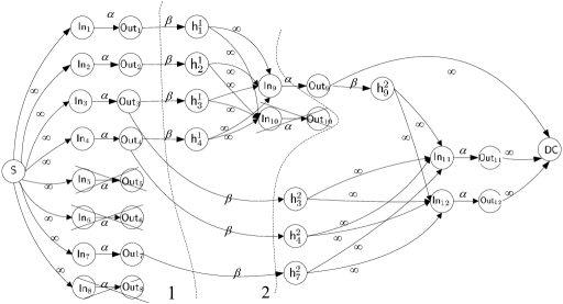
Figure 1: An example for cut-capacity in broadcast repair.

IV Storage Capacity

According to [2], the capacity of the single source multicast network is given by the minimum value of the cut-capacity between the source node and any of the destinations. Therefore, the storage capacity of a particular WDSS instance $I$ is given by

$$C^{\prime}(I)=\min_{\mathsf{DC}}\min_{\mathcal{X}:\mathsf{S}-\mathsf{DC}\text{~{}cut}}C(\mathcal{X}),$$ (2)

where the first minimum is taken over all legitimate choices of $\mathsf{DC}$ under the instance $I$. The storage capacity, $C_{\text{storage}}$, of a WDSS can be obtained by minimizing $C^{\prime}(I)$ over all its possible instances, i.e.,

$$C_{\text{storage}}=\min_{I}C^{\prime}(I).$$ (3)

Consider an arbitrary instance of the WDSS. Regard the initialization stage as round 0 and let $\mathcal{V}_{0}\triangleq\mathcal{N}$. For rounds $s\in\mathcal{T}\triangleq\{1,2,\ldots,T\}$, let $\mathcal{A}_{s}\triangleq\{\mathsf{h}_{i}^{s}:i\in\mathcal{H}_{s}\}$ be the set of auxiliary vertices in round $s$, and $\mathcal{V}_{s}\triangleq\mathcal{A}_{s}\cup\{\mathsf{In}_{j},\mathsf{Out}_{j}:j\in\mathcal{R}_{s}\}$ be the set of all vertices in round $s$. Then $\mathcal{V}_{0}\cup\mathcal{V}_{1}\cup\cdots\cup\mathcal{V}_{T}$ contains all the vertices except the source and the destinations in the graph.

To obtain the cut-capacity of an arbitrary $\mathsf{S}-\mathsf{DC}$ cut $\mathcal{X}^{\prime}$, we examine the in-edges of all the vertices in $\mathcal{V}_{0}\cup\mathcal{V}_{1}\cup\cdots\cup\mathcal{V}_{T}$, and express the cut-capacity as a sum of $T+1$ terms:

$$C(\mathcal{X}^{\prime})=\sum_{0\leq s\leq T}C_{\vartriangle,s}(\mathcal{X}^{\prime}),$$ (4)

where

$$C_{\vartriangle,s}(\mathcal{X}^{\prime})\triangleq\sum_{i\in\mathcal{X}^{\prime},j\in\mathcal{V}_{s}\cap\overline{\mathcal{X}^{\prime}}}u_{ij}$$

is called the cut-capacity contribution of the vertices in $\mathcal{V}_{s}$. When there is no ambiguity, we may simply write it as $C_{\vartriangle,s}$. For example, in Fig. 1, the cut denoted by left side of line 2 has cut-capacity equal to $C_{\vartriangle,0}+C_{\vartriangle,1}+C_{\vartriangle,2}=0+\alpha+3\beta$.

Now we investigate $C_{\vartriangle,s}(\mathcal{X}^{\prime})$ for $0\leq s\leq T$. First, consider the case where $s=0$. Since there is no auxiliary vertex in repair round 0, we have $C_{\vartriangle,0}=x_{0}\alpha,$ where $x_{0}$ is the number of storage nodes in round 0 such that its in-vertex is in $\mathcal{X}^{\prime}$ and out-vertex is in $\overline{\mathcal{X}^{\prime}}$.

Second, consider the case where $s\in\mathcal{T}_{1}^{\prime}$, where $\mathcal{T}_{1}^{\prime}\triangleq\{s\in\mathcal{T}:\mathcal{A}_{s}\cap\mathcal{X}^{\prime}\neq\emptyset\}$. In other words, $s\in\mathcal{T}_{1}^{\prime}$ if there exists at least one $\mathsf{h}_{i}^{s}$ in $\mathcal{X}^{\prime}$. We investigate the three classes of vertices in $\mathcal{V}_{s}$, i.e., auxiliary vertices, in-vertices, and out-vertices, one by one. For the auxiliary vertices, denote the number of $\mathsf{h}_{i}^{s}$’s such that it is in $\overline{\mathcal{X}^{\prime}}$ and its parent vertex $\mathsf{Out}_{i}$ is in $\mathcal{X}^{\prime}$ by $z_{s}$. For the in-vertices, we only need to consider the case where all of them are in $\mathcal{X}^{\prime}$, for otherwise, the cut-capacity contribution would be infinite as all its in-edges have infinite capacity and at least one of its parent vertex is in $\mathcal{X}^{\prime}$. For the out-vertices, denote the number of them in $\overline{\mathcal{X}^{\prime}}$ by $x_{s}$. Then we have $C_{\vartriangle,s}=x_{s}\alpha+z_{s}\beta.$ An illustration of this case is shown in Fig. 2

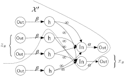
Figure 2: An illustration of case where $s\in\mathcal{T}_{1}^{\prime}$.

Third, consider the case where $s\in\mathcal{T}_{2}^{\prime}\triangleq\mathcal{T}\setminus\mathcal{T}_{1}^{\prime}$. By definition of $\mathcal{T}_{2}^{\prime}$, all $\mathsf{h}_{i}^{s}$’s are in $\overline{\mathcal{X}^{\prime}}$. For the auxiliary vertices, denote the number of $\mathsf{h}_{i}^{s}$’s such that its parent vertex $\mathsf{Out}_{i}$ is in $\mathcal{X}^{\prime}$ by $y_{s}$. For all the in-vertices, since their parent vertices are all in $\overline{\mathcal{X}^{\prime}}$, their cut-capacity contribution is zero, no matter they are in $\mathcal{X}^{\prime}$ or $\overline{\mathcal{X}^{\prime}}$. The cut-capacity contribution of all the in-vertices is 0. For the out-vertices, denote the number of them such that $\mathsf{Out}_{j}\in\overline{\mathcal{X}^{\prime}}$ and its parent vertex $\mathsf{In}_{j}\in\mathcal{X}^{\prime}$ by $v_{s}$. we have $C_{\vartriangle,s}=v_{s}\alpha+y_{s}\beta.$ An illustration of this case is shown in Fig. 3

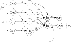
Figure 3: An illustration of case where $s\in\mathcal{T}_{2}^{\prime}$.

Combining the above three cases and according to (4), we have

$$C(\mathcal{X}^{\prime})=x_{0}\alpha+\sum_{s\in\mathcal{T}_{1}^{\prime}}\left(x_{s}\alpha+z_{s}\beta\right)+\sum_{s\in\mathcal{T}_{2}^{\prime}}(v_{s}\alpha+y_{s}\beta).$$

Now consider a special cut $\mathcal{X}$, which is constructed from $\mathcal{X}^{\prime}$ as follows. Initially, let $\mathcal{X}$ be the same as $\mathcal{X}^{\prime}$. For $s\in\mathcal{T}_{1}^{\prime}$, move all $\mathsf{h}_{i}^{s}$’s into $\mathcal{X}$, and then $z_{s}$ becomes zero. Furthermore, since $\mathsf{h}_{i}^{s}$’s child vertices are all in round $s$, moving all $\mathsf{h}_{i}$’s into $\mathcal{X}$ will not affect the cut-capacity contribution of other rounds. For $s\in\mathcal{T}_{2}^{\prime}$, move all $\mathsf{In}_{j}$’s into $\overline{\mathcal{X}}$, and $v_{s}$ becomes zero. Again, since $\mathsf{In}_{j}$’s child vertex $\mathsf{Out}_{j}$ is in the same round, moving $\mathsf{In}_{j}$ will not affect the cut-capacity contribution of other rounds. We have

$$C(\mathcal{X}^{\prime})\geq C(\mathcal{X})=x_{0}\alpha+\sum_{s\in\mathcal{T}_{1}}x_{s}\alpha+\sum_{s\in\mathcal{T}_{2}}y_{s}\beta,$$ (5)

where $\mathcal{T}_{1}$ is the index set of repair rounds whose auxiliary vertices are all in $\mathcal{X}$, and $\mathcal{T}_{2}$ is the index set of repair rounds whose auxiliary vertices are all in $\overline{\mathcal{X}}$. Note that $\mathcal{T}_{1}\cup\mathcal{T}_{2}=\mathcal{T}$. Since $x_{s}$ is the number of vertices such that it is in $\overline{\mathcal{X}}$ and its parent vertex is in $\mathcal{X}$, let $x_{s}=0$ for $s\in\mathcal{T}_{2}$.

For any round $s$, let the number of out-vertices in $\overline{\mathcal{X}}$ be $m_{s}$. By definition, we have $m_{s}=x_{s},\;\;\text{if }s\in\mathcal{T}_{1}\cup\{0\}$ and

$$0\leq m_{s}\leq r,\;\;\text{if }s\in\mathcal{T}_{2}.$$ (6)

Furthermore, we define

$$m_{s}^{*}=\left\{\begin{array}[]{ll}x_{s},&s\in\mathcal{T}_{1}\cup\{0\}\\ r,&s\in\mathcal{T}_{2}.\end{array}\right.$$ (7)

The following result is established by finding bounds for $x_{s}$ and $y_{s}$.

Theorem 1.

The storage capacity of WDSS$(n,k,d,r,\alpha,\beta,T)$ $C_{\text{storage}}$ is lower bounded by $C_{LB}(T)\triangleq$

$$\min_{\boldsymbol{x},\mathcal{T}_{1}}\left\{x_{0}\alpha+\sum_{s\in\mathcal{T}_{1}}x_{s}\alpha+\sum_{s\in\mathcal{T}\setminus\mathcal{T}_{1}}\max(0,d-\sum_{i=0}^{s-1}m_{i}^{*})\beta\right\},$$ (8)

where the minimization is taken over $\mathcal{T}_{1}\subseteq\mathcal{T}=\{1,2,\ldots,T\}$ and

$$0\leq x_{0}\leq n,$$ (9)

$$0\leq x_{s}\leq r,\text{ for }s\in\mathcal{T}_{1},$$ (10)

$$k\leq\sum_{s\in\mathcal{T}_{1}\cup\{0\}}x_{s} +(|\mathcal{T}|-|\mathcal{T}_{1}|)r\leq k+r.$$ (11)

Proof.

Since any arbitrary data collector $\mathsf{DC}_{s,\mathcal{K}}$ is able to connect to $k$ out-vertices through links with infinite capacity, for any cut with finite cut-capacity, we must have

$$\sum_{s\in\mathcal{T}_{1}\cup\{0\}}x_{s}+\sum_{s\in\mathcal{T}_{2}}m_{s}\geq k.$$ (12)

It is clear that $x_{s}$ must also satisfy (9) and (10).

There are $d$ helper nodes for newcomers in round $s$ and at most $\sum_{i=0}^{s-1}m_{i}$ of them have their out-vertices in $\overline{\mathcal{X}}$. Therefore, we have

$$y_{s}\geq\max(0,d-\sum_{i=0}^{s-1}m_{i}),\text{ for }s\in\mathcal{T}_{2}.$$

By (5), the cut-capacity of a given cut is bounded below by

$$x_{0}\alpha+\sum_{s\in\mathcal{T}_{1}}x_{s}\alpha+\sum_{s\in\mathcal{T}_{2}}\max(0,d-\sum_{i=0}^{s-1}m_{i})\beta.$$

Note that the above expression is a monotonic decreasing function of each $m_{i}$. If (12) is originally satisfied, increasing the value of each $m_{i}$ will not violate it. By (6), the above expression is minimized when $m_{s}^{*}=r$ for $s\in\mathcal{T}_{2}$. Then (12) becomes

$$\sum_{s\in\mathcal{T}_{1}\cup\{0\}}x_{s}+\sum_{s\in\mathcal{T}_{2}}r\geq k.$$ (13)

Let $(\boldsymbol{x}^{*},\mathcal{T}_{1}^{*})$ achieves the minimum of (8), where $\boldsymbol{x}^{*}\triangleq(x_{0}^{*},x_{1}^{*},\ldots,x_{T}^{*})$. The minimum value of (8) is thus equal to

$$\sum_{s\in\mathcal{T}_{1}\cup\{0\}}x_{s}^{*}\alpha+\sum_{s\in\mathcal{T}_{2}}\max(0,d-\sum_{i\in\mathcal{T}_{1}\cup\{0\},\atop i<s}x_{i}^{*}-\sum_{i\in\mathcal{T}_{2},i<s}r)\beta.$$ (14)

Suppose to the contrary that

$$\sum_{s\in\mathcal{T}_{1}\cup\{0\}}x_{s}^{*}+\sum_{s\in\mathcal{T}_{2}}r>k+r.$$ (15)

We claim that we can always find another feasible solution which achieves a lower objective function value than (14). To see this, consider the last repair round $s^{\prime}\in\mathcal{T}$ which has strictly positive value of $m_{s^{\prime}}^{*}$. If $m^{*}_{T}>0$, then $s^{\prime}=T$. Otherwise, we have $m_{s^{\prime}}^{*}>0$ and $m_{s}^{*}=0$ for all $s>s^{\prime}$. By definition of $m^{*}_{s}$, we have $s\in\mathcal{T}_{1}$ for all $s>s^{\prime}$. If $s^{\prime}\in\mathcal{T}_{1}$, we can set $x_{s^{\prime}}^{*}=0$ to strictly reduce the value of the expression in (14). Since $x_{s^{\prime}}^{*}\leq r$, the new setting will not violate constraint (13). Therefore, (15) cannot hold. If $s^{\prime}\in\mathcal{T}_{2}$, we move $s^{\prime}$ from $\mathcal{T}_{2}$ to $\mathcal{T}_{1}$, and set $m_{s^{\prime}}^{*}=0$. The value in (14) will not be increased while constraint (13) will still be satisfied due to the assumption in (15). We then repeat the above argument and find another new index $s^{\prime}$. Due to constraint (13), $\boldsymbol{x}^{*}$ cannot be the zero vector, which leads to a contradiction. Hence, (15) does not hold and we must have (11). ∎

In the following theorem, we show the tightness of the lower bound when $T$ is finite.

Theorem 2.

When $T$ is finite, the lower bound in Theorem 1 is tight when $n\geq k+2r$.

Proof.

Let $(\boldsymbol{x}^{*},\mathcal{T}_{1}^{*})$ be an optimal solution to the minimization in Theorem 1. We prove that the bound is tight by constructing an instance $I^{*}$ with a $\mathsf{DC}^{*}$ and a cut $\mathcal{X}^{*}$ such that the cut-capacity $C(\mathcal{X}^{*})$ is exactly $C_{LB}(T)$.

The instance $I^{*}$ is constructed as follows. First, in stage 0, choose any $r$ nodes in $\mathcal{N}$ and let them fail. For stage $s\in\mathcal{T}_{1}^{*}$, choose any $r-x_{s}^{*}$ nodes in $\mathcal{R}_{s}$ and any $x_{s}^{*}$ active nodes in $\mathcal{N}$ and let them fail right before stage $s+1$. For stage $s\in\mathcal{T}_{2}^{*}$, choose any $r$ active nodes in $\mathcal{N}$ and let them fail right before stage $s+1$. We can always find such a failure pattern since there are $r$ nodes in $\mathcal{R}_{s}$ for every $s$, and the accumulated number of failed nodes in $\mathcal{N}$ is

$$r+\sum_{s\in\mathcal{T}^{*}_{1}}x_{s}^{*}+\sum_{s\in\mathcal{T}_{2}^{*}}r\leq k+2r\leq n,$$

where the first inequality follows from (11) and the second inequality follows our assumption in Theorem 2. Select any $x_{0}^{*}$ active nodes from $\mathcal{N}$ and denote them by $\mathcal{M}_{0}$. Denote the active nodes in $\mathcal{R}_{s}$ by $\mathcal{M}_{s}$. In other words, for $s\in\mathcal{T}_{1}^{*}\cup\{0\}$, $\mathcal{M}_{s}\subseteq\mathcal{R}_{s}$ and $|\mathcal{M}_{s}|=x_{s}^{*}$; for $s\in\mathcal{T}_{2}^{*}$, $\mathcal{M}_{s}=\mathcal{R}_{s}$.

Next, we specify the helper nodes for each repair round. The helper nodes for repair round $i$, for $i=1,2,\ldots,s$, are chosen first from $\mathcal{M}_{0}$, then from $\mathcal{M}_{1}$, and so on, until $d$ helper nodes are chosen. If $\sum_{i=0}^{s-1}|\mathcal{M}_{i}|<d$, the remaining helper nodes are chosen arbitrarily from the active nodes in $\mathcal{N}$. The existence of such a helper pattern is validated by

$$n-r-|\mathcal{M}_{1}|-\dots-|\mathcal{M}_{s-1}|\geq d-|\mathcal{M}_{0}|-\dots-|\mathcal{M}_{s-1}|,$$

where the left side is the number of active nodes in $\mathcal{N}$ after stage $s-1$, and the right side is the number of required helper nodes in $\mathcal{N}$. The inequality holds because $n-r\geq d$.

Finally, consider $\mathsf{DC}_{T,\mathcal{K}^{*}}$, which comes after the repair round $T$ and connects to $\mathcal{K}^{*}\subseteq\mathcal{M}_{0}\cup\mathcal{M}_{1}\cup\dots\cup\mathcal{M}_{T}$. Note that there is such a DC, since according to (11), $|\mathcal{M}_{0}\cup\mathcal{M}_{1}\cup\dots\cup\mathcal{M}_{T}|\geq k$.

The cut $\mathcal{X}^{*}$ is constructed as follows: For $s\in\{0\}\cup\mathcal{T}_{1}^{*}$, put $\mathsf{Out}_{i}$, for $i\in\mathcal{M}_{s}$, into $\overline{\mathcal{X}^{*}}$, and all the remaining vertices in round $s$ into $\mathcal{X}^{*}$. Vertices in these repair rounds contribute $x_{0}^{*}\alpha+\sum_{s\in\mathcal{T}_{1}^{*}}x_{s}^{*}\alpha$ to the cut-capacity. For $s\in\mathcal{T}_{2}^{*}$, put all vertices in round $s$ into $\overline{\mathcal{X}^{*}}$. Vertices in these repair rounds contribute $\sum_{s\in\mathcal{T}_{2}^{*}}\max\Big{\{}0,d-x_{0}^{*}-\sum_{i\in\mathcal{T}_{1}^{*},i<s}x_{i}^{*}-\sum_{i\in\mathcal{T}_{2}^{*},i<s}r\Big{\}}\beta$ to the cut-capacity. Summing up the cut-capacity contribution of all the vertices, we get $C_{LB}(T)$, showing that the bound in Theorem 1 is tight. ∎

Furthermore, the following result significantly reduces the dimension of the minimization problem. The proof is omitted due to space limitation.

Theorem 3.

When $T\geq k+r$, we have $C_{LB}(T)=C_{LB}(k+r)$.

V Comparison with Cooperative Repair

We compare broadcast repair with cooperative repair when $T\geq k+r$ and $k=ur$, where $u$ is an integer larger than 1. Both repair process is triggered after the number of failed storage nodes accumulate to $r$. Consider the two points, minimum storage (MS) point, which corresponds to the best storage efficiency, and the minimum repair-transmission bandwidth (MT) point, which corresponds to the minimum repair-transmission bandwidth on the trade-off curve between repair-transmission bandwidth and storage (see Fig.4 shown in next page for example). In cooperative repair, the repair-transmission bandwidth is equal to the repair bandwidth. According to [6], the MS point and the MT point are $(\tau_{\text{MSC}},\alpha_{\text{MSC}})=(\frac{d+r-1}{k(d+r-k)},\frac{1}{k}),\text{ and }(\tau_{\text{MTC}},\alpha_{\text{MTC}})=\frac{2d+r-1}{k(2d+r-k)}(1,1),$ respectively. We can also derive the MS point and the MT point in broadcast repair, which are: $(\tau_{\text{MSB}},\alpha_{\text{MSB}})=\big{(}\frac{d}{k(d+r-k)},\frac{1}{k}\big{)},\text{ and }(\tau_{\text{MTB}},\alpha_{\text{MTB}})=\frac{2d}{k(2d+r-k)}(1,1),$ respectively. Since $r>1$, broadcast repair outperforms cooperative repair at these two points.

In Fig.4 (shown in next page), we plot the tradeoff curves of the two repair schemes with parameters $C_{\text{Storage}}=1,d=9$, $k=4$ and $r=2$. As a benchmark, we also plot the single-node repair, in which the repair is triggered whenever there is a single node failure. As reported in [6], cooperative repair performs better than single-node repair due to the benefit of node cooperation. However, it performs worse than broadcast repair, since it does not exploit the broadcast nature of the wireless medium.

References

- [1] A. G. Dimakis, P. B. Godfrey, Y. Wu, M. J. Wainwright, and K. Ramchandran, “Network coding for distributed storage systems,” IEEE Trans. Inf. Theory, vol. 56, no. 9, pp. 4539–4551, Sep. 2010.
- [2] R. Ahlswede, N. Cai, S.-Y. R. Li, and R. W. Yeung, “Network information flow,” IEEE Trans. Inf. Theory, vol. 46, no. 4, pp. 1204–1216, Jul. 2000.
- [3] Y. Wu, “Existence and construction of capacity-achieving network codes for distributed storage,” IEEE J. on Selected Areas in Commun., vol. 28, no. 2, pp. 277–288, Feb. 2010.
- [4] P. Hu, K. W. Shum, and C. W. Sung, “The fundamental theorem of distributed storage systems revisited,” Hobart, Australia, Nov. 2014, pp. 65–69.
- [5] Y. Hu, Y. Xu, X. Wang, C. Zhan, and P. Li, “Cooperative recovery of distributed storage systems from multiple losses with network coding,” IEEE J. on Selected Areas in Commun., vol. 28, no. 2, pp. 268–276, Feb. 2010.
- [6] K. W. Shum and Y. Hu, “Cooperative regenrerating codes,” IEEE Trans. Inf. Theory, vol. 59, no. 11, pp. 7229–7258, Nov. 2013.
- [7] A. G. Dimakis and K. Ramchandran, “Network coding for distributed storage in wireless networks,” in Networked Sensing Information and Control. Springer US, Apr. 2008, pp. 115–134.
- [8] C. Gong and X. Wang, “On partial downloading for wireless distributed storage networks,” IEEE Trans. on Signal Processing, vol. 60, no. 6, pp. 3278–3288, Jun. 2012.
- [9] M. Gerami, M. Xiao, J. Li, C. Fischione, and Z. Lin, “Repair for distributed storage systems in packet erasure networks,” http://arxiv.org/abs/1405.3188, May 2014.
- [10] M. Gerami, M. Xiao, and M. Skoglund, “Partial repair for wireless caching networks with broadcast channels,” IEEE Wireless Communications Letters, vol. 4, no. 2, pp. 145–148, Apr. 2015.