Storm Detection by Visual Learning Using Satellite Images

Abstract

Computers are widely utilized in today’s weather forecasting as a powerful tool to leverage an enormous amount of data. Yet, despite the availability of such data, current techniques often fall short of producing reliable detailed storm forecasts. Each year severe thunderstorms cause significant damage and loss of life, some of which could be avoided if better forecasts were available. We propose a computer algorithm that analyzes satellite images from historical archives to locate visual signatures of severe thunderstorms for short-term predictions. While computers are involved in weather forecasts to solve numerical models based on sensory data, they are less competent in forecasting based on visual patterns from satellite images. In our system, we extract and summarize important visual storm evidence from satellite image sequences in the way that meteorologists interpret the images. In particular, the algorithm extracts and fits local cloud motion from image sequences to model the storm-related cloud patches. Image data from the year 2008 have been adopted to train the model, and historical thunderstorm reports in continental US from 2000 through 2013 have been used as the ground-truth and priors in the modeling process. Experiments demonstrate the usefulness and potential of the algorithm for producing more accurate thunderstorm forecasts.

I Introduction

I-A Background

The numerical weather prediction (NWP) approach has been applied to weather forecasting since the 1950s [1], when the first computer ENIAC was invented [2]. John von Neumann, a pioneering computer scientist and meteorologist, first applied the primitive equation models [3] on ENIAC. Since then meteorologists have produced reliable weather forecasts, and they have continued to refine the numerical models, thereby improving the NWP in recent decades. Today, the model of the European Centre for Medium-range Weather Forecasts (ECMWF) and the United States’ Global Forecast System (GFS) are two of the most accurate NWP models. At the 500 hPa geopotential height (HGT) level of the atmosphere, both models are reported to have annual mean correlation coefficients of nearly 0.9 for 5-day forecasts [4]. Other models, such as UK Met Office Unified model [5], Météo-France ARPEGE-Climat model [6], and Canada Meteorological Centre model [7], are developed and play important roles in global and regional weather predictions.

Even though NWP can effectively produce accurate weather forecasts of the general weather pattern, it is not always reliable in the prediction of extreme weather events, such as severe thunderstorms, hail storms, hurricanes, and tornadoes, which cause a significant amount of damage and loss of life every year worldwide. Unreliable predictions, either miss or false alarm ones, could cause massive amounts of loss to the society. The most well-known failed prediction is the Great Storm of 1987 in UK [8]. The Met Office was criticized for not predicting the storm timely. More recently, the landfall of 2012 Hurricane Sandy in the northeastern US was not correctly predicted by the National Hurricane Center until two days before it came ashore [9]. In January 2015, the impact of winter storm Juno was overestimated by the US National Weather Service [10]. Several cities in US East Coast suffered from unnecessary travel bans and public transportation closures. Much of the loss of life and property due to improper precautions to severe weather events could be avoided with more accurate (for both severity and location) weather forecasts.

The numerical methods used in NWP can efficiently process large amounts of meteorological measurements. However, a major drawback of such methods is that they are sensitive to noise and initial inputs due to the complexity of the models [11, 12]. As a result, although nowadays we have powerful computers to run complex numerical models, it is difficult to get accurate predictions computationally, especially in the forecasts of severe weather. To some extent, they do not interpret the data from a global point of view at a high cognitive level. For instance, meteorologists can make good judgments of the future weather conditions by looking at the general cloud patterns and developing trends from a sequence of satellite images by using geographical knowledge and their experience of past weather events [13, 14]; numerical methods do not capture such high-level clues. Additionally, historical weather records provide valuable references for making weather forecasts, but numerical methods do not make best use of them.

To address this weakness of numerical models, we develop a computational weather forecast method that takes advantage of both the global visual clues of satellite data and the historical records. In particular, we try to find synoptic scale features of mid-latitude thunderstorms (to be specified later in Section I-C) by computer vision and machine learning approaches. It is worth mentioning that the purpose of this work is not to replace numerical models in forecasting. Instead, by tackling the problem using different data sources and modeling methodologies, we aspire to develop a method that can potentially be used side-by-side with and complement numerical models.

We analyze the satellite imagery because it provides important clues as meteorologists view evolving global weather systems. Unlike conventional meteorological measures such as temperature, humidity, air pressure, and wind speed, which directly reflect the physical conditions at the sensors’ locations, the visual information in satellite images is captured remotely from the orbit, which means a larger geographic coverage with good resolution. The brightness in an infrared satellite image indicates the temperature of the cloud tops [15] and therefore reveals information about the top-level structure of the cloud systems. Manually interpreting such visual information, we can trace the evidence that corresponds to certain weather patterns, particularly those related to severe thunderstorms. Moreover, certain cloud patterns can be evident in the early stage of storm development. As a result, the satellite imagery are very helpful to meteorologists in their work.

Human eyes can effectively capture the visual patterns related to different types of weather events. The interpretation requires a high level understanding of meteorological knowledge, which has been difficult for computers. However, because the broad spatial and temporal coverage of the satellite images produces too much information to be fully processed, there is an emerging need for a computerized way to analyze the satellite images automatically. Therefore researchers are seeking computer vision algorithms to automatically process and interpret the visual features from the satellite images, aiming to help meteorologists better analyze and predict weather events. Traditional satellite image analysis techniques include cloud detection with complex backgrounds [16], cloud type classification [17, 18, 19], detection of cloud overshooting top [20, 21], and tracking of cyclone movement [22]. These approaches, however, only capture local visual features without utilizing many high-level global visual patterns, and overlook their development over time, which provides more clues for weather forecasts. With the development of advanced computer vision algorithms, some recent techniques put more focus on the analysis of cloud motion and deformation [23, 24, 25, 26]. In these approaches, cloud motions are estimated to match and compare cloud patches between adjacent images in a sequence. In this paper, the proposed algorithm also uses cloud motion estimation in image sequences. It is different from existing work in that it extracts and models certain patterns of cloud motion, in addition to capturing the cloud displacement.

Historical satellite data archives as well as meteorological observations are readily available for recent years. By analyzing large amounts of past satellite images and inspecting the historical weather records, our system takes advantage of big data to produce storm alerts given a certain query image sequence. The result provides an alternative prediction that can validate and correct the conventional forecasts. It can be embedded into an integrative or information fusion system, as suggested in [27], to work with data and decisions from other sources and produce more improved storm forecasts.

I-B The Dataset

For our research, we acquired all of the GOES-M [28] satellite imagery for the year of 2008, which was an active year containing abundant severe thunderstorm cases for us to analyze. The GOES-M satellite moves on a geostationary orbit and was continually facing the North America area during that year. In addition to the imagery data, each record contains navigation information, which helps us map each image pixel to its real geo-location. The data is multi-spectral and contains five channels covering different ranges of wavelengths, among which we adopted channel 3 (6.5-7.0$\mu$m) and channel 4 (10.2-11.2$\mu$m) in our analysis because these two infrared channels are available both day and night. Both channels are of 4 km resolution and the observation frequency is four records per hour, i.e., about 15 minutes between the adjacent images. To make sure two adjacent images in a sequence have a noticeable difference, we sampled the original sequence and used a sub-sequence with a 2-frames-per-hour frame rate. We select the 30-minute sampling interval because the algorithm is based on the optical flow analysis between to adjacent image frames. We need both evident enough visual difference and relatively good temporal resolution. The 30-minute interval is a empirical selection that considers both factors. In the rest of the paper, every two adjacent images in a sequence we refer to are 30 minutes away without specifying.

Using the imagery and navigation data blocks in each raw data entry, we reconstruct satellite images by an equirectangular projection [29]. The pixel mapping from the raw imagery data to the map coordinate is computed by the navigation data with transformation defined by [28]. The map resolution is set to be 4 km (per pixel), which best utilizes the information of the raw data. We reconstruct the aligned images within the range of 60°W to 124°W in longitude and 20°N to 52°N in latitude, which covers the Continental US (CONUS) area. Hereafter all the image related computations in our approach are performed on the reconstructed images, on which the geo-location of each pixel is directly accessible.

We studied the relationship between satellite images and severe thunderstorms, which may include hailstorms and tornados. To relate the satellite data with severe thunderstorms, we retrieved the storm report data from the NOAA National Weather Service, where all the time and locations of storms inside the United States since the year of 2000 are archived. The records act as ground-truth data in the training and provide geographic and temporal priors for the system to make decisions.

I-C Synoptic-scale Visual Storm Signatures

Being evidently visible on the satellite imagery, synoptic-scale (spanning several hundred kilometers) storm features are studied in this paper. Particularly, we are interested in the synoptic-scale features of the mid-latitude ($30^{\circ}$-$60^{\circ}$ in latitude) thunderstorms located outside of the Hadley cell [30] of the atmospheric circulation because storms cooccurring with these features are one of the major components of storms in the CONUS and other densely populated areas around the world.

Synoptically, one important atmospheric feature helpful for locating thunderstorms is the subtropical jet stream, which is the high-altitude (10-16 km) westerly wind near the boundary between the Hadley cell and the Ferrel cell; in other words, the cold and warm air masses. Jet streams move in a meandering path from west to east, a direction of movement caused by the Coriolis effect [31]. In the northern hemisphere, elongated cold air masses with low pressure, namely “troughs”, will have a dip in the jet stream extending southward at various longitudes around the earth while in other locations a ridge of higher pressure with warm air will send the jet stream bulging northward. The east side of a trough, which has a southwest to northeast oriented jet stream, is a region of active atmospheric storminess [32], where cold and warm air masses collide. Though jet streams themselves are invisible, they can be revealed by thick cumulus clouds gathering in the unsettled trough regions and areas of clouds spreading northeastward along the east side of a trough. As a result, an elongated cloud-covered area along a southwest to northeast direction is a useful large-scale clue for us to locate storms. Fig. 1 shows a GOES-M channel-4 image taken on February 5, 2008. Clearly in the mid-latitude region the southern boundary of the cloud band goes along a smooth curve, which indicates the jet stream (sketched in dashed line). Usually the cloud-covered areas to the northwest side of such an easily-perceivable jet stream are susceptible to storms. In this case, severe thunderstorms developed two hours after the time of the image in the boxed area of the figure. Based on our observation, a large proportion of storms in the CONUS area have similar cloud appearances as in this example. As a result, finding jet streams in the satellite image is important for storm prediction [33].

A jet stream travels along a large-scale meandering path, whose wavelength is about 60^∘ to 120^∘ of longitude long, as wide as a whole continent. The full wavelength is therefore usually referred to as a long wave. The trough within a long wave only tells us a general large region that is vulnerable to storms. To locate individual storm cells more precisely, meteorologists look for more detailed smaller scale cloud patterns caused by short waves traveling through the long wave. Short waves are synoptic scale features with the wavelength of the order of 1,000 km, and indicate the disturbance of the mid or upper part of the atmosphere. Horizontally seen from a satellite image, they appear as smaller waves in the long wave trough. In many cases, we can observe clouds in “comma shapes” [34, 35] in short waves, i.e., such a cloud has a round shape due to the circular wind in its vicinity and a short tail towards the opposite direction of its translation. A comma-shaped cloud patch indicates a turbulent area of rising air often leading to convection (thunderstorms), especially if it lies on the boundary between cold and warm air masses. Fig. 1 shows an example of a comma-shaped cloud. A storm area is marked by an square in the tail of the comma shape in the figure. Because of its distinctive pattern, the comma shape has been one of the most utilized signature when meteorologists review satellite images for thunderstorms.

It is necessary to mention that the comma shape is still a signature in the synoptic scale and therefore used for generally locating a storm system rather than individual storms. In other words, groupings of thunderstorms tend to have a comma shape and the shape is used as a first approximation of where severe weather is most likely to occur.

The visual cloud patterns introduced above can often be detected from a single satellite image. However, a single image is not sufficient to provide all the crucial information about the dynamic of a storm system. The cloud shapes are not always clear due to the irregular nature of clouds. In addition, the evolution of storm systems, including cloud areas emerging, disappearing, and deforming, cannot be revealed unless different satellite images in a sequence are compared.

In practice, an important step in producing weather forecasts is to review satellite images, during which process meteorologists typically review a series of images, rather than a single one, to capture critical patterns. They use the differences between the key visual clues (e.g., key points, edges, etc.) to track the development of storm systems and better locate the jet streams and comma shapes, among other features. As mentioned in [36], human heuristics are helpful in improving weather forecasts. Following such guideline, our algorithm attempts to simulate meteorologists’ cognitive processes in analyzing temporally adjacent satellite image frames. In particular, two types of motions are regarded crucial to the storm visual patterns: the global cloud translation with the jet stream and the local cloud rotations producing the comma shapes. We consider both types of motions for extracting synoptic storm signatures.

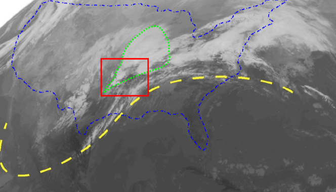
Figure 1: A sample GOES-M satellite channel 4 image taken at 16:02 (GMT) on February 5, 2008. The boxed area underwent a severe thunderstorm later on that day. The jet stream (marked in dashed curve) can be implied from the distribution of clouds. The storm area is covered by a comma-shaped cloud patch (surrounded by dashed boundary) in the trough region.

I-D Objectives

The algorithm proposed in this paper aims at assisting the prediction of severe thunderstorms from a different perspective from the NWP. As an initial attempt in this direction, we focus on short-term severe thunderstorm prediction. Synoptical scale features abstracted from known visual storm patterns as aforementioned are extracted from satellite images and used as clues to locate regions where thunderstorms tend to happen in the near future. Machine learning is involved in the classification of candidate storm regions by inspecting historical thunderstorm data. The regions, as extracted from synoptical scale features, are not necessarily associated one-to-one with storms, i.e., a region may contain several storms and each storm needs to be more precisely located by other techniques. The algorithm in fact simulates meteorologists’ cognition process when reviewing satellite images as a part of the weather prediction process. It could be a helpful tool in automating and refining the current weather prediction. It can also be used to provide assistance to meteorologists so that they can be more efficient and less exhausting.

I-E Outline

The rest of the paper is organized as follows. Section II introduces the approach to extract storm signatures and construct storm features. Section III reports the approach and results of the machine learning module that accepts or rejects the extracted storm features. In particular, quantitative benchmarks of the classifier and qualitative case studies that applies the whole workflow are given to demonstrate the effectiveness of the proposed algorithm. Finally, we present the future work and conclude the paper in Section IV.

II Storm Feature Extraction

Our algorithm extracts synoptic-scale visual thunderstorm features from satellite images. The cloud motion observed from image sequences is analyzed in depth. In order to simulate human cognition and let computers perceive comma shapes introduced earlier, the visual signatures are further abstracted into basic cloud motion components: translation and rotation. Several properties and measurements related to these two components are extracted from cloud motions and analyzed in the following steps.

Fig. 2 illustrates the workflow of the whole system. We employ the optical flow between every two adjacent satellite images to capture the cloud motion and discover vortex areas that could potentially trigger storms. Using the historical storm records, vortex features are constructed and a storm classifier is trained. Given an arbitrary query image sequence, vortexes are extracted in the same way and then categorized by the classifier.

In particular, for the feature extraction operations, which will be applied both to the training data and the query data, two steps are carried out. The system first estimates a dense optical flow field describing the cloud motion between adjacent image frames. Second, local vortexes are identified with the optical flow and vortex descriptors are constructed. The vortex descriptors combine information from both the visual features and the historical storm records. The following subsections describe details of these steps.

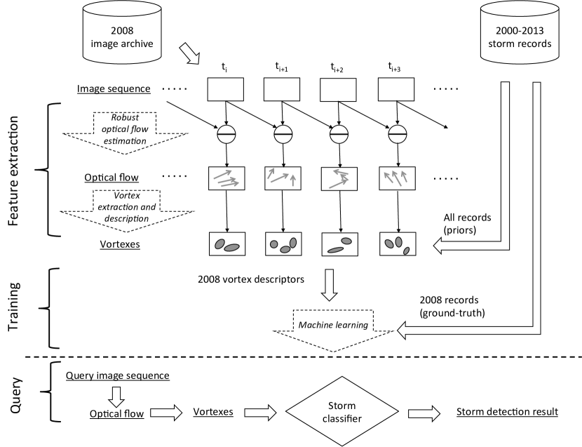
Figure 2: Workflow of the storm detection system. Optical flows between adjacent image frames are estimated and vortexes are extracted base on the flows. Vortex descriptors are then constructed using both the visual information and historical storm records. Machine learning is performed on the vortex descriptors for the storm detection.

II-A Robust Optical Flow Estimation

Optical flow is a basic technique for motion estimation in image sequences. Given two images $I_{t}(x,y)$ and $I_{t+1}(x,y)$, the optical flow $\vec{F}_{t}(x,y)=\{U_{t}(x,y),V_{t}(x,y)\}$ defines a mapping for each pixel $g:(x,y)\mapsto(x+U_{t}(x,y),y+V_{t}(x,y))$, so that $I_{t}(g(x,y))\approx I_{t+1}(x,y)$. The vector field $\vec{F}_{t}(x,y)$ can be therefore regarded as the pixel-wise motions from image $I_{t}(x,y)$ to $I_{t+1}(x,y)$. Several approaches for optical flow estimation have been proposed based on different optimization criteria [37, 38, 39]. In this work we adopt the pyramid Lucas-Kanade algorithm [40] to estimate a dense optical flow field between every two neighboring image frames.

The GOES-M satellite is in a geostationary orbit and thus remains over the same point on the earth at all times. As a result, the only objects moving along a satellite image sequence are the clouds and the optical flow between two images indicates the cloud motion. However, the non-rigid and dynamic nature of clouds makes the optical flow estimation noisy and inaccurate. Fig. 3(a) shows the optical flow estimation result of a satellite image in respect to its previous frame in the sequence. Though the result correctly reflects the general cloud motion, flows in local areas are usually noisy and do not precisely describe the local motions. As to be introduced later, the optical flow properties adopted in this work involve the gradient operation of the flow field. Thus it is important to get reliable and smooth optical flow estimation. To achieve this goal, we both pre-process the images and post-process the estimation results. Before calculating the optical flow between two images, we first enhance both of them using the histogram equalization technique [41]. As a result, more fine details on the images are enhanced for better optical flow estimation.

After the initial optical flow estimation, we smooth the optical flow by applying an iterative update operation based on the Navier-Stokes equation [42] for modeling fluid motions. Given a flow field $\vec{F}(x,y)$, the equation describes the evolving of the flow over time $t$:

$$\frac{\partial\vec{F}}{\partial t}=(-\vec{F}\cdot\nabla)\vec{F}+\nu\nabla^{2}\vec{F}+\vec{f}\;,$$ (1)

where $\nabla=(\frac{\partial}{\partial x},\frac{\partial}{\partial y})$ is the gradient operator, $\nu$ is the viscosity of the fluid, and $\vec{f}(x,y)$ is the external force applied at the location $(x,y)$.

The three terms in Eq. (1) correspond to the advection, diffusion, and outer force of the flow field respectively. In the method introduced in [43], an initial flow field is updated to a stable status by iteratively applying these three transformations one by one. Compared with a regular low-pass filtering to the flow field, this approach takes into account the physical model of fluid dynamics, and therefore better approximates the real movement of a flow field. We adopt a similar strategy to smooth the optical flow in our case. The initial optical flow field $\vec{F_{t}}(x,y)$ is iteratively updated. Within each iteration the time is incremented by a small interval $\Delta t$, and there are three steps to get $\vec{F}_{t+\Delta t}(x,y)$ from $\vec{F}_{t}(x,y)$:

1. add force: $\vec{F}_{t+\Delta t}^{(1)}=\vec{F}_{t}+\vec{f}\Delta t$ ;

2. advect: $\vec{F}_{t+\Delta t}^{(2)}=adv(\vec{F}_{t+\Delta t}^{(1)},-\Delta t)$ ;

3. diffuse: $\vec{F}_{t+\Delta t}=FFT^{-1}(FFT(\vec{F}_{t+\Delta t}^{(2)})e^{-\nu k^{2}\Delta t})$ .

The first step is simply a linear increment of the flow vectors based on the external force. In the second step, the advection operator $adv(\cdot)$ uses the flow $\vec{F}_{t+\Delta t}^{1}(x,y)$ at each pixel $(x,y)$ to predict its location $(x_{t-\Delta t},y_{t-\Delta t})$ $\Delta t$ time ago, and updates $\vec{F}_{t+\Delta t}^{(2)}(x,y)$ by $\vec{F}_{t+\Delta t}^{(1)}(x_{t-\Delta t},y_{t-\Delta t})$. In the last step, the diffusion operation is a low-pass filter applied in the frequency domain, where $k$ is the distance from a point to the origin, and the bandwidth of the filter is determined by the pre-defined fluid viscosity $\nu$ and $\Delta t$ (to be specified later). We do not enforce the mass conservation like the approach in [43] because the two-dimensional flow field corresponding to the cloud movement is not necessarily divergence free. In fact, we use the divergence as a feature for storm detection in the following procedures.

After several iterations of the update, the flow field converges to a stable status and becomes smoother. The iteration number is typically not large, and we find that the final result is not very sensitive to the parameters $\nu$ and $\Delta t$. In our system we set the iteration number to 5, the fluid viscosity $\nu$ to 0.001, and time interval $\Delta t$ to 1. The noisy optical flow estimation from the previous stage is treated as the external force field $\vec{f}$, and initially $\vec{F}_{t}=0$. Fig. 3(b) shows the smoothed flow field (i.e., $\vec{F}_{t+5\Delta t}$) from the noisy estimation (Fig. 3(a)). Clearly the major motion information is kept and the flow field is smooth for further analysis.

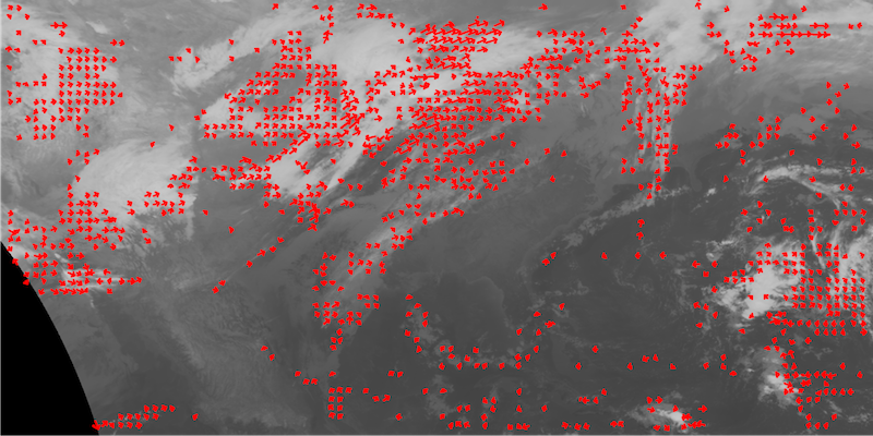
(a) Noisy optical flow estimation

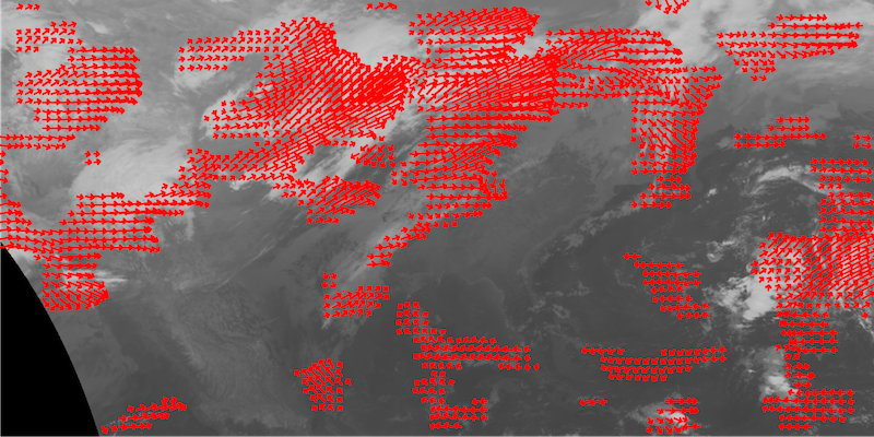
(b) Smoothed optical flow

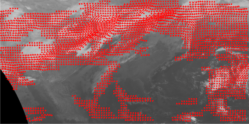
(c) Divergence-free component of the smoothed flow

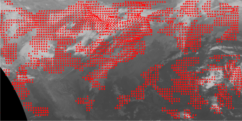
(d) Vorticity-free component of the smoothed flow

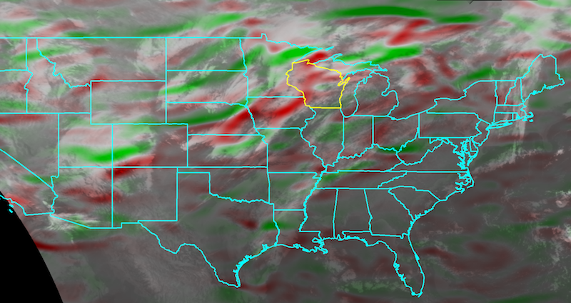
(e) Magnitude of vorticity

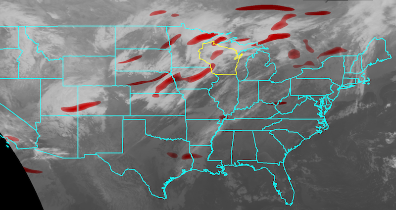
(f) Vortex cores and their expansions

Figure 3: Sample results of the optical flow analysis. GOES-M satellite images covering the continental US area are analyzed (to avoid showing too many missing pixels on the southwest corner, a small stripe of US west coast is not shown on the figures, though these pixels are included in our analysis). Between two adjacent frames (with 30 minutes’ interval) in a satellite image sequence, the optical flow from the former frame to the latter one is estimated and processed. The results are plotted on the second frame. Only large enough flow vectors are drawn on figure (a-d). (a) The optical flow estimated by the Lucas-Kanade algorithm. (b) The smoothed optical flow by applying an iterative update based on the Navier-Stokes equation. (c) The divergence-free component of the smoothed flow field. (d) The vorticity-free component of the smoothed flow field. (e) Visualization of the vorticity. Vorticity vectors of the 2D flow field are perpendicular to the image plane. Pixels with vorticity vectors toward the viewer (counter-clockwise rotations) are tinted in green color; and the pixels with vorticity away from the viewer (clockwise rotations) are tinted in red color. The saturation of color means the magnitude of the corresponding vorticity vector. (f) Vortex regions detected by the $Q$-criterion. For visualization purpose (to avoid displaying too a large missing corner at the lower-left, not all areas in CONUS are shown on the above images.

II-B Flow Field Vortex Extraction

As introduced in Section I, the rotating and diverging of local cloud patches are two key signatures for storm detection. In the flow field, these two kinds of evidence are embodied by the vorticity and divergence. The vorticity of a vector field $\vec{F}(x,y)=\{U(x,y),V(x,y)\}$ is defined as:

$$\vec{\omega}(x,y) =\nabla\times\vec{F}(x,y)$$ (2)

$$=\left(\frac{\partial}{\partial x},\frac{\partial}{\partial y},\frac{\partial}{\partial z}\right)\times(U(x,y),V(x,y),0)$$

$$=\left(\frac{\partial V(x,y)}{\partial x}-\frac{\partial U(x,y)}{\partial y}\right)\vec{z}\;;$$

and the divergence is defined as:

$$\text{div}\vec{F}(x,y) =\nabla\cdot\vec{F}(x,y)$$ (3)

$$=\left(\frac{\partial}{\partial x},\frac{\partial}{\partial y}\right)\cdot(U(x,y),V(x,y))$$

$$=\frac{\partial U(x,y)}{\partial x}+\frac{\partial V(x,y)}{\partial y}\;.$$

It has been proven that for a rigid body, the magnitude of vorticity at any point is twice the angular velocity of its self rotation [44] (the direction of the vorticity vector indicates the rotation’s direction). In our case, even though the cloud is non-rigid, we can regard the vorticity at a certain point as a description of the local rotation.

To better reveal the rotation and divergence, we apply the Helmholtz-Hodge Decomposition [45] to decompose the flow field to a solenoidal (divergence-free) component and a irrotational (vorticity-free) component. Fig. 3(c) and Fig. 3(d) visualize these two components respectively. In both figures, areas with densely overlapped vectors plotted are the places with high vorticity or divergence.

The divergence-free component of the flow field is useful for detecting vortexes. On this component, we inspect the local deformation tensor

$$\nabla\vec{F}=\left[\begin{matrix}{\partial U}/{\partial x}&{\partial V}/{\partial x}\\ {\partial U}/{\partial y}&{\partial V}/{\partial y}\end{matrix}\right]\;,$$

which can be decomposed to the symmetric (strain) part $S=\frac{1}{2}({\nabla\vec{F}+\nabla\vec{F}^{T}})$ and the asymmetric (rotation) part $\Omega=\frac{1}{2}({\nabla\vec{F}-\nabla\vec{F}^{T}})$. The $Q$-criterion introduced by [46] takes the difference of their norms:

$$Q=\frac{1}{2}(\|\Omega\|^{2}-\|S\|^{2})=\frac{1}{4}\|\vec{\omega}\|^{2}-\frac{1}{2}\|S\|^{2}\;,$$ (4)

where $\|\cdot\|$ is the Frobenius matrix norm. The $Q$-criterion measures the dominance of the vorticity. When $Q>0$, i.e., the vorticity component dominates the local flow, the corresponding location is regarded to be in a vortex region. Fig. 3(e) and Fig. 3(f) visualize the vorticity and $Q$-criterion of the flow field in Fig. 3(c). In Fig. 3(e), pixels are tinted by the corresponding magnitude of vorticity, and different colors mean different rotating directions. In Fig. 3(f), the vortex regions are highlighted in red. Clearly only pixels with a dominant vorticity component are selected as vortexes by the $Q$-criterion. It is apparent that these vortexes are more prone to be located inside the storm area (highlighted by yellow boundaries) than the removed high-vorticity pixels. It is also observed that the vortexes are typically in narrow bending comma shapes as described in Section I-C. Therefore, they are properly to be regarded as the potential storm elements.

II-C Vortex Descriptor

Not all the vortex regions in Fig. 3(f) are related to storms. As a result we built a descriptor for each extracted vortex and apply it to a machine learning module (to be introduced later). We introduce the vortex descriptor in this subsection.

Denoting a certain vortex region in a satellite image as $\Phi$ and the area of $\Phi$ as $\Pi(\Phi)$, the following visual clues, both static ones from a single image and dynamic ones from the optical flow with respect to the previous image frame, are considered in our approach.

1. Mean channel 3 brightness:

   $$w_{1}(\Phi)=\frac{\sum_{(x,y)\in\Phi}I^{(3)}(x,y)}{\Pi(\Phi)}\;,$$

   where $I^{(3)}(x,y)$ is the brightness of pixel $(x,y)$ in the channel 3 image.

2. Mean channel 4 brightness:

   $$w_{2}(\Phi)=\frac{\sum_{(x,y)\in\Phi}I^{(4)}(x,y)}{\Pi(\Phi)}\;,$$

   where $I^{(4)}(x,y)$ is the brightness of pixel $(x,y)$ in the channel 3 image.

3. Mean optical flow intensity:

   $$w_{3}(\Phi)=\frac{\sum_{(x,y)\in\Phi}\|\vec{F}(x,y)\|}{\Pi(\Phi)}\;,$$

   where $\vec{F}(x,y)=(U(x,y),V(x,y))$ is the optical flow at pixel $(x,y)$ computed between the previous and current image frames.

4. Mean optical flow direction:

   $$w_{4}(\Phi)=\frac{\sum_{(x,y)\in\Phi}\|\theta(x,y)\|}{\Pi(\Phi)}\;,$$

   where $\theta(x,y)=\tan^{-1}\left(\frac{V(x,y)}{U(x,y)}\right)$ is optical flow $\vec{F}(x,y)$’s direction.

5. Mean vorticity on the solenoidal optical flow component:

   $$w_{5}(\Phi)=\frac{\sum_{(x,y)\in\Phi}\omega(x,y)}{\Pi(\Phi)}\;,$$

   where $\omega(x,y)$ is the vorticity value of the solenoidal component of optical flow $\vec{F}(x,y)$ (sign of the value indicates the vorticity’s direction).

6. Mean divergence on the irrotational optical flow component:

   $$w_{6}(\Phi)=\frac{\sum_{(x,y)\in\Phi}\text{div}\vec{F}(x,y)}{\Pi(\Phi)}\;,$$

   where $\vec{F}(x,y)$ is the divergence of the irrotational component of optical flow $\vec{F}(x,y)$.

7. Maximal $Q$-value of the vortex:

   $$w_{7}(\Phi)=\max_{(x,y)\in\Phi}{Q(x,y)}\;,$$

   where $Q(x,y)$ is defined in Eq. (4).

We also considered the spatial and temporal distributions of the storms that occurred in the CONUS from 2000 to 2013 using all the historical storm records through these years. This is shown in Fig. 4. We divided the CONUS area into $4^{\circ}\times 4^{\circ}$ grids. Inside each grid, we count the occurrence of storms around each given date (e.g., July 4th) in the history. Storms that occurred from 5 days before to 5 days after the queried date in each year are counted (e.g., for July 4, storms from June 29 to July 9 in every year, a total of 154 days, are included). Denoting the total storm count in grid $(i,j)$ (the grid counted $i$-th from the left and $j$-th from the top) for date $d$ is $N_{d}(i,j)$ , the average storm density in the grid is $\rho_{d}(i,j)=\tfrac{N_{d}(i,j)}{154}$.

To describe the storm prior for vortex $\Phi$ (extracted from date $d$), we took the average storm densities of the pixels it covers:

$$w_{8}(\Phi)=\frac{\sum_{(x,y)\in\Phi}\phi_{d}(T(x,y))}{\Pi(\Phi)}\;,$$

where $T:(x,y)\mapsto(i,j)$ is a mapping from the pixel $(x,y)$ to the grid index $(i,j)$ it belongs to.

With all the features introduced above, for vortex $\Phi$ we constructed a vortex descriptor $X(\Phi)=(w_{1},w_{2},w_{3},w_{4},w_{5},w_{6},w_{7},w_{8})$. Descriptors of training data are fed into a machine learning algorithm, and eventually we obtain a classifier $C(\cdot)$. For an arbitrary vortex $\Phi$, $Y(\Phi)=C(X(\Phi))$ is the predicted status calculated by the classifier. We introduce the machine learning approach in the next section.

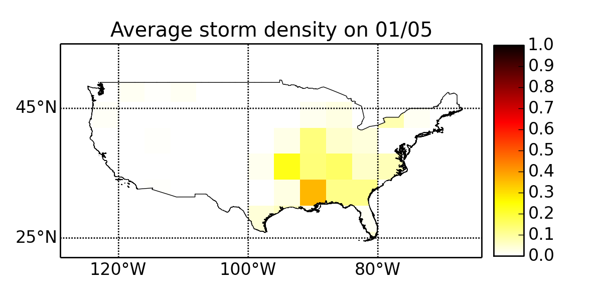
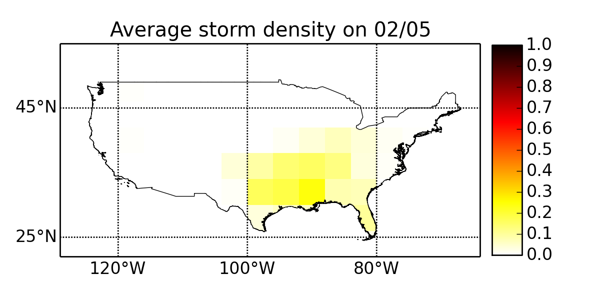
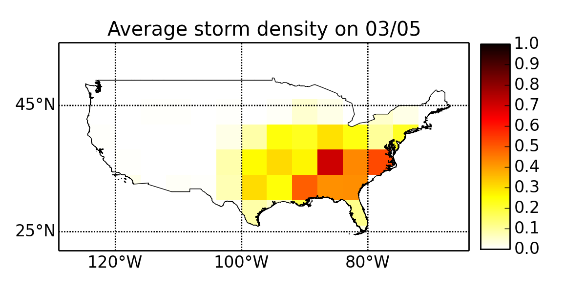
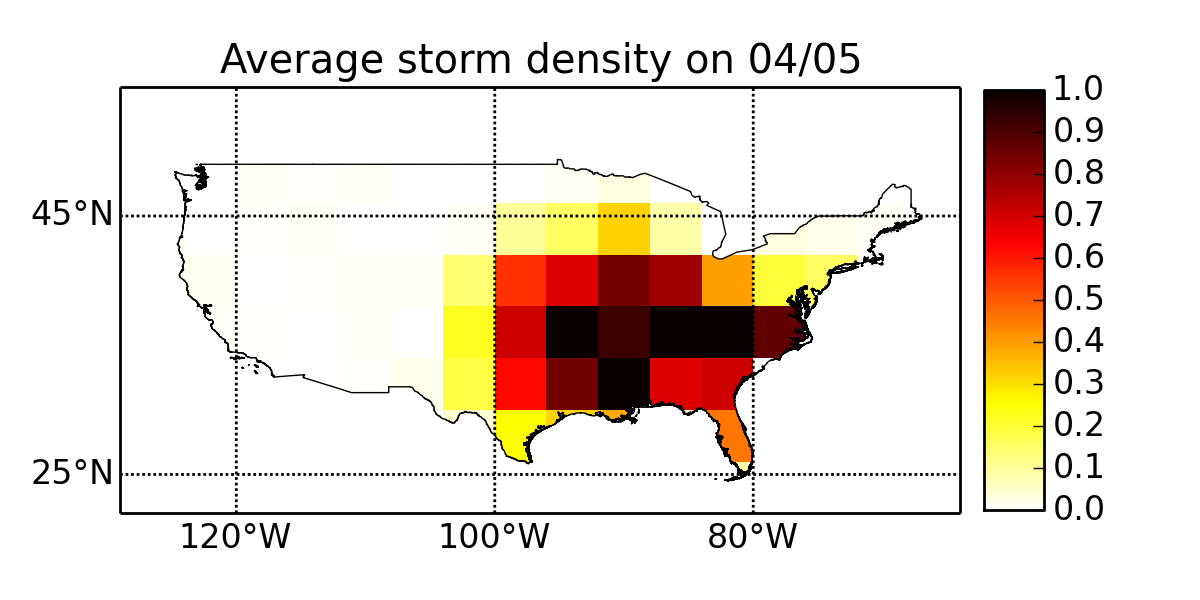
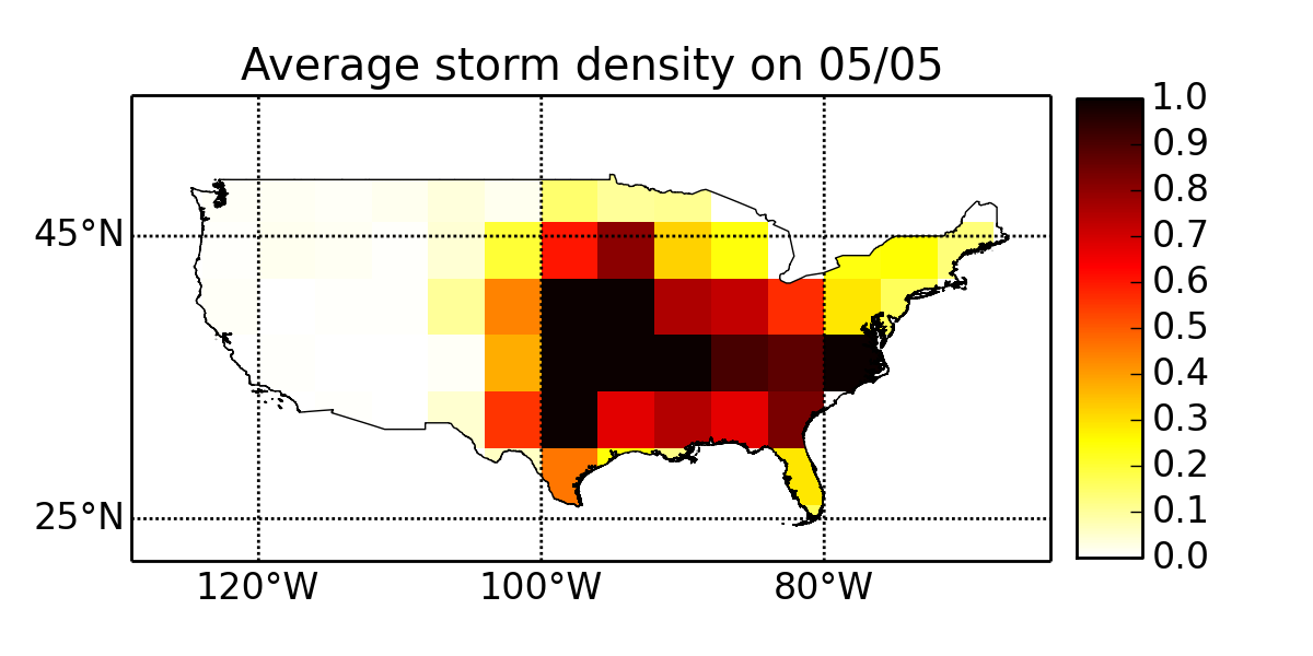
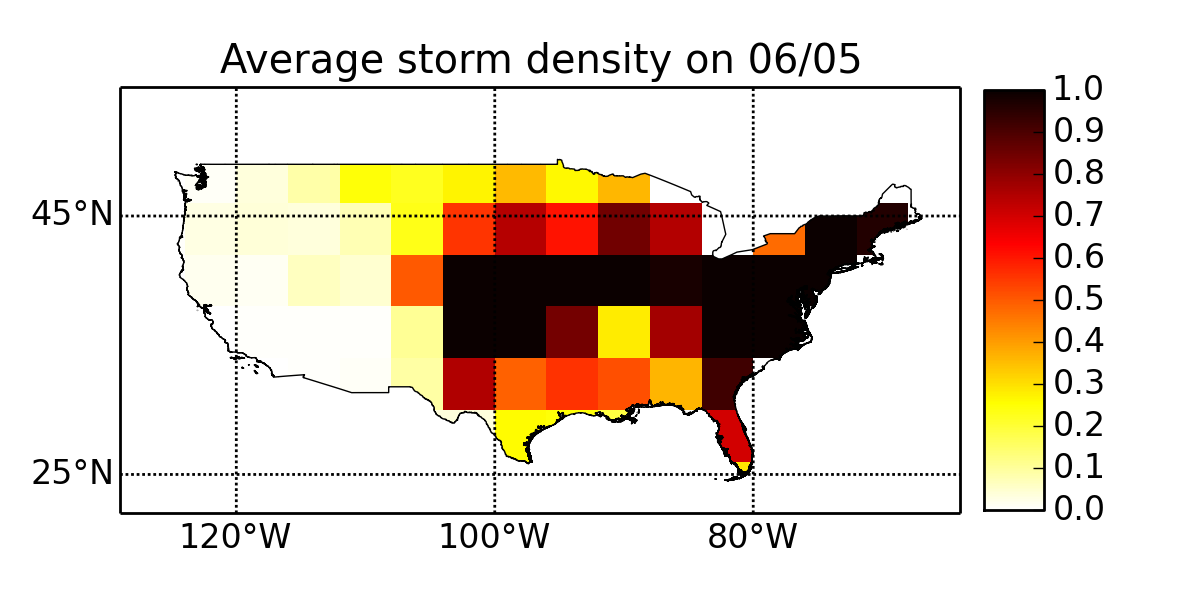
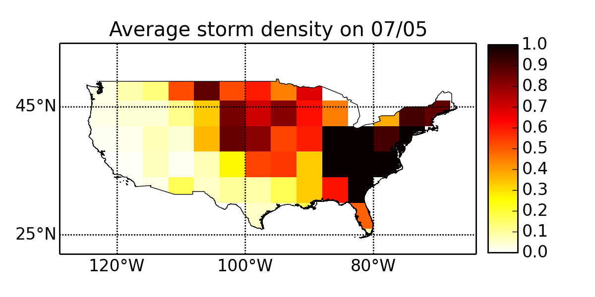
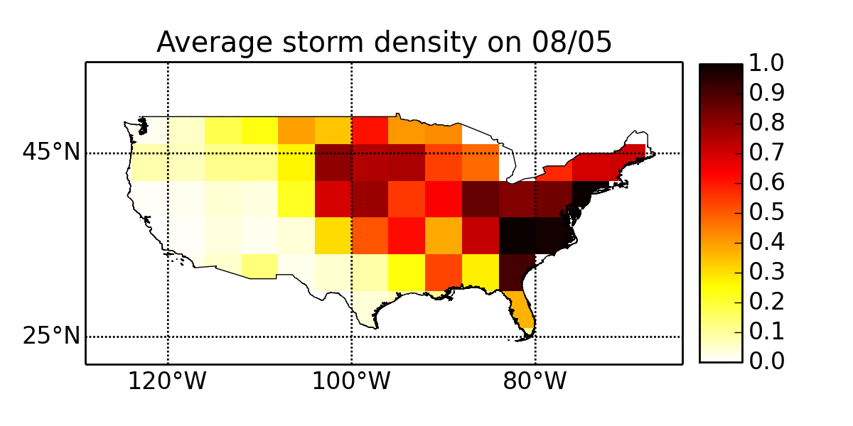
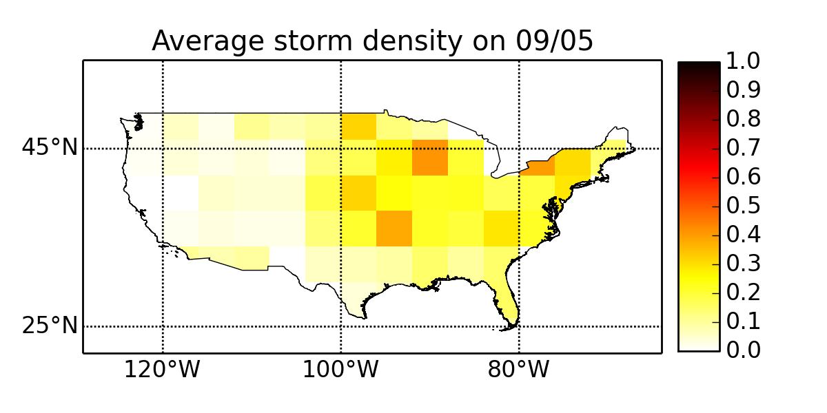
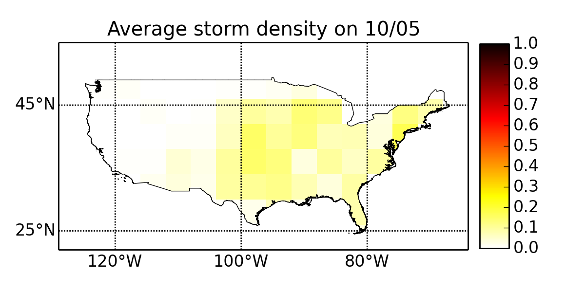
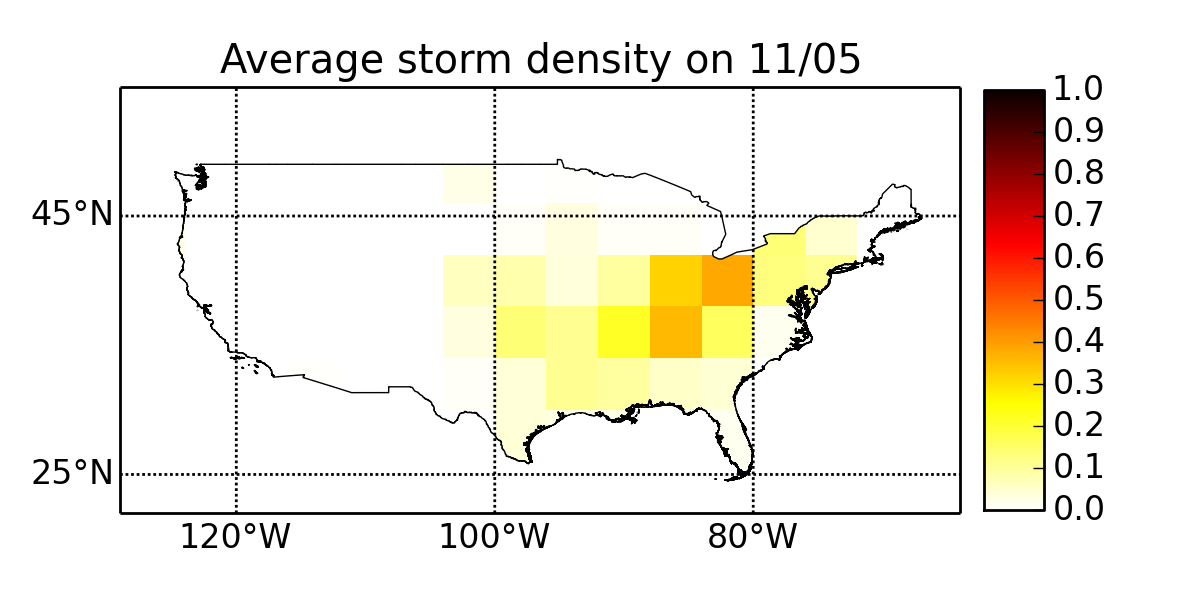
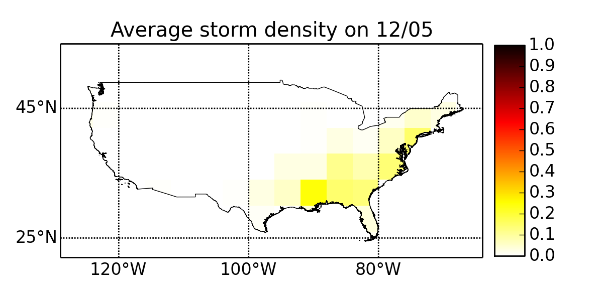
Figure 4: Average storm densities (number of storms per 30,000 $\text{km}^{2}$) for the fifth day of each month in US continent. Darker color means higher storm density. The statistics are based on the historical records from 2000 to 2013. Around each given date (+/-5 days), we count the total number of storms reported in each state across the past 14 years. The numbers are then divided by the total number of days and the areas of corresponding states to calculate the average densities.

III Storm System Classification and Detection

The vortex regions with large $Q$ values correspond to regions with strong cloud rotations and our approach extracts them as vortexes. However, they are not necessarily related to the storms because the cloud rotation is only one aspect of a weather system. In order to create reliable storm detection, we embedded these vortexes and their descriptors into a machine learning framework. Using the descriptors and ground-truth labels of the extracted candidate vortex regions, a classifier was trained to distinguish storm-related vortexes from other vortexes.

III-A Training Vortexes and Ground-truth Labels

We extracted vortexes from 2008 GOES-M satellite images and used the storm reports in the same year to assign a ground-truth label for each vortex in the CONUS. A classifier is trained to associate the vortex features with the storm labels. Image sequences in the first ten days of each month are used for training and those from the 18th to the 22nd days of each month are used for testing (so that the weather systems in the training and testing data are relatively far apart and independent). In order to get enough difference yet not to lose too much detail, we choose the sampling interval between every two images in a sequence to be 30 minutes.

We used the historical storms to assign ground-truth labels to detected vortexes. We denote the historical storm database as $\mathscr{D}$ and each storm entry as $(u_{i},v_{i},t_{i})$ where $(u_{i},v_{i})$ is the location (latitude and longitude values in degrees) and $t_{i}$ is the starting time of the storm. Assuming a vortex is detected at location $(u,v)$ and time $t$, if at least one record $(u_{i},v_{i},t_{i})\in\mathscr{D}$ within $3^{\circ}$ of latitude and longitude exists between the moments $t-0.5hr$ and $t+2hr$ (i.e. $\|u_{i}-u\|<3^{\circ}\text{ and }\|v_{i}-v\|<3^{\circ}\text{ and }t-0.5hr\leq t_{i}\leq t+2hr$), the vortex is assigned with a positive (storm-related) label; otherwise it is assigned with a negative (no-storm) label. We only assigned labels for vortexes inside the CONUS. For vortexes outside of the CONUS, we had no historical data indicating whether or not they are storm-related, so we did not use them for training and testing.

On the 120 selected days (10 for each month), a total of 8,527 storm-related vortexes were discovered by the above method. We randomly selected the same number of vortexes in the CONUS that were not storm-related from these days. A binary classifier is then trained on the 17,054 training vortex samples.

III-B Random Forest Classifier

We trained a random forest classifier [47] using the training data to distinguish storm-related vortexes from vortexes not affiliated with a storm. The features for each vortex are described in Section II-C and the ground-truth is defined in Section III-A.

Using the training data, the random forest learns rules to determine whether a vortex of certain descriptor causes storms. The random forest is essentially an ensemble learning algorithm that makes predictions by combining the results of multiple individual decision trees trained from random subsets of the training data. We chose this approach because it has been found to outperform a single classifier (e.g., SVM). In fact, this strategy resembles the ensemble forecasting [48] approach in numerical weather prediction, where multiple numerical results with different initial conditions are combined to make a more reliable weather forecast. For both numerical and statistical weather forecasting approaches, the ensemble approaches help to improve the prediction qualities.

III-C Testing Vortex Samples and Testing Methods

To develop a benchmark for the performance of the vortex classifier, we used image sequences from the 18th to the 22nd days of each month in 2008 as the testing data. On each selected day, the image sequence (with a 30-minute interval) from 10:00 GMT to 18:00 GMT is used to extract dynamic cloud vortexes. The test dataset contains a total of 48,698 vortexes, among which 781 are labeled as positive, and the rest 47,917 samples are negative. The descriptors of these vortexes are classified by the classifier. We then evaluate the classification results in two ways.

Firstly, we assigned the testing vortexes with ground-truth labels in the same way as how the training ground-truth labels are assigned. The predicted storm status for each test vortex is compared with the ground-truth. In this way the classification accuracy for single vortexes are evaluated. Table I presents the classification performance of both the training data (by cross validation) and the testing data. The classifier shows consistent performances on both the training set and the test set. To demonstrate the effect of including geographic storm priors in the classification, we also trained and tested the random forest classifiers only on the visual features and the storm density separately. Clearly none of the visual features and the historical storm density standalone performs well alone. Combining visual features with the storm density significantly enhances the classification performance.

TABLE I: Classification Performance and Contributions of Visual Features and Historical Priors

		All features	Visual only	Prior only
Training set (cross validation)	Overall	83.3%	68.8%	76.1%
	Sensitivity	89.6%	67.4%	74.8%
	Specificity	76.9%	70.3%	77.3%
Testing set	Overall	80.3%	67.4%	77.3%
	Sensitivity	82.1%	47.2%	77.4%
	Specificity	80.2%	67.7%	71.2%

Note: Training set contains 5,876 storm-related and 5,876 no-storm vortex regions from 120 days in 2008. 10-fold cross validation is performed in the evaluation. Testing set contains 2,706 storm-related cells and 7,773 no-storm cells from 60 days far away from the training data. The feature vector for each vortex is composed by both visual features and storm priors (see Section II-C). Beside the merged features (results shown in the first column), we test the two types of features separately (results shown in the second and third columns).

Secondly, we evaluated the classifier’s ability to predict the future locations of storms. Instead of comparing each vortex’s classification result with its ground-truth label, which reflects its status within the period of $(t-0.5hr,t+2hr)$ ($t$ is the timestamp of the vortex), we observed how much time in advance a storm can be detected by our algorithm. Given a testing vortex extracted at the location $(u,v)$ and time $t$, we find the earliest time $t^{\prime}=T(u,v,t)$ that a neighboring storm $(u^{\prime},v^{\prime},t^{\prime})\in\mathscr{D}$ developed since two hours before $t$, i.e.,

$$t^{\prime}=\min_{t_{i}}{\left\{(u_{i},v_{i},t_{i})\in\mathscr{D}\text{ and }\|u_{i}-u\|<3^{\circ}\text{ and }\|v_{i}-v\|<3^{\circ}\text{ and }t_{i}>t-2hr\right\}}\;.$$

The value $\Delta t=T(u,v,t)-t$ indicates the time difference between an observed vortex and the first storm to form nearby storm. For a vortex with $\Delta t>0$, a future storm is predicted if the classifier can label a vortex as storm-related. The percentages of storms predicted for vortexes with different $\Delta t>0$ are shown in Fig. 5. The results show that the proposed algorithm can effectively predict future storms within several hours of the detection of vortexes and the prediction reliability increases as $\Delta t$ decreases. Particularly, it shows a reasonable prediction rate for the development of nearby storms within a period of 4 hours after the observation of visual vortexes in satellite images.

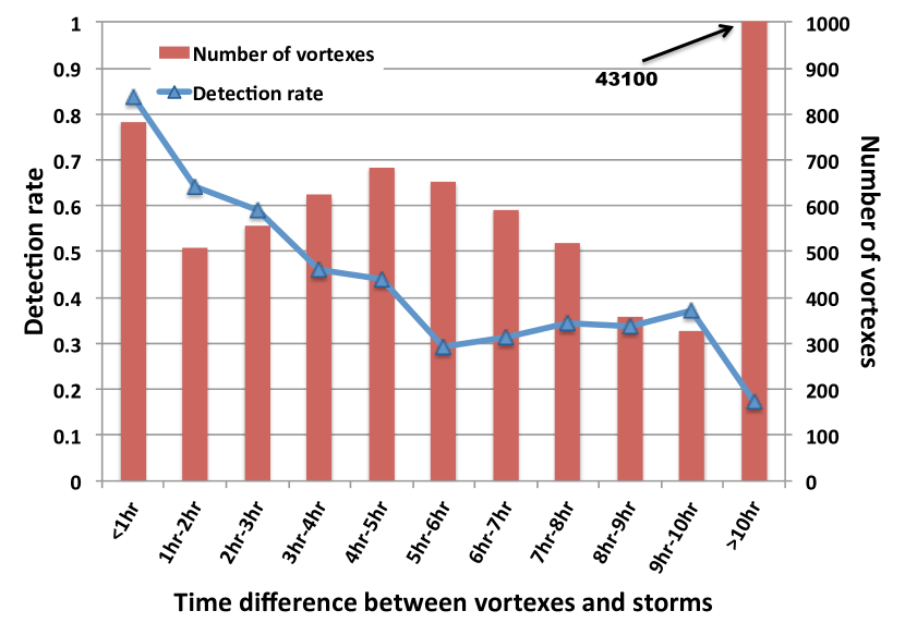
Figure 5: Storm detection rate with different amounts of time in advance. The distribution of the time differences ($\Delta t$) between the testing vortex samples and storms are plotted in red bars (the last bar is not fully shown because it is much higher than others). And the percentages of vortexes categorized as storms with different $\Delta t$ are plotted in a blue curve. The figure shows that the predictivity of the classifier is generally reliable within few hours of time in advance. The storm detection rate decreases as the time difference becomes longer.

It is necessary to emphasize that the classification is performed on already extracted candidate vortex regions where local clouds are rotating. Most of the cloud-covered regions on the satellite images without obvious rotational motions have been already eliminated before the algorithm proceeds to the classification stage. Therefore in practice the system achieves a good overall precision for detecting the storms. In addition, the classification results for individual vortex regions can be further corrected and validated based on their spatial and temporal neighboring relationships.

III-D Case Study

To demonstrate the usefulness of the proposed vortex detection and classification algorithm in real scenarios, we present several case studies where our algorithm is applied for automatic storm detection from satellite images.

Three different cases are presented and the results are visualized in Fig. 6 (one row for each case). An active storm reporting day , a clear storm-free day, and a cloudy storm-free day are selected to demonstrate the adaptiveness of our algorithm. These three image sequences are not included in the training process of the storm classifier. In Fig. 6, automatically detected vortexes are filled with colors on each image. Vortexes classified as storms are colored in red, and the green vortexes are categorized as storm-free cases by the machine learning module. The US state boundaries are drawn on each image to show the alignment between the satellite images and the geo-coordinate system. In particular, boundaries of states affected by storms are highlighted by warm colors from red to yellow. The highlighting color indicates how long after the observation storms were reported in the corresponding states. As the color turns to yellow, the highlighted states are affected by storms further in the future. Specifically, the red color means an ongoing storm and the yellow color means a storm 6 hours after the observation time. Fig. 6 only shows the results on the first three image frames of each case due to space limitation. Each test image sequence in fact contains more than three frames, and the storm detection results are consistent in the subsequent frames for each case.

The first case is from May 25, 2008, which was an active storm day, when several severe storms hit the Midwest US. An obvious cloud vortex system is visible on the satellite images and it is related to storms reported in nearby states. Our algorithm captures all the major vortexes from the satellite image sequence, and correctly categories most of them as storms. The result also shows the capability of the proposed algorithm to assist in short-term storm forecasting. In most cases there will be storms detected around regions where storms were reported shortly thereafter.

Different from the first case, the second case is strongly negative in that little clouds and vortexes can be perceived from the images. Results on the second row of Fig. 6 shows that no storm is predicted because few clouds and vortexes can be captured by the feature extraction stage of our algorithm. In this case, it is easy for the algorithm to make correct decisions.

In the third case, several cloud systems can be observed above the CONUS, and several vortexes are detected by the optical flow analysis. In reality, even though some cloud vortex systems look dominant on the image sequence, there is no severe storm reported on that day. Results shown on the third row of Fig. 6 demonstrate that the machine learning module successfully avoids labeling the detected cloud vortexes as storms. This shows that the system does not over-predict the occurrence of storms. This benefit is also validated by the standalone test for the classifier showing that specificity of the classifier is as high as its sensitivity.

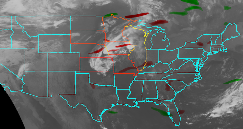
(a) 2008/05/25 12:15 GMT

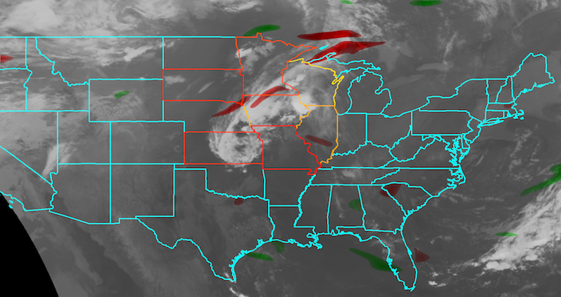
(b) 2008/05/25 12:45 GMT

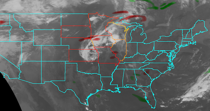
(c) 2008/05/25 13:15 GMT

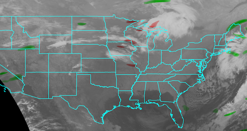
(d) 2008/09/18 12:15 GMT

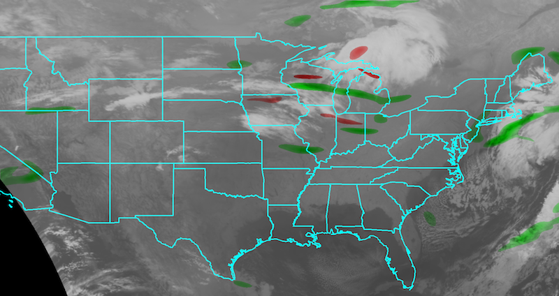
(e) 2008/09/18 12:45 GMT

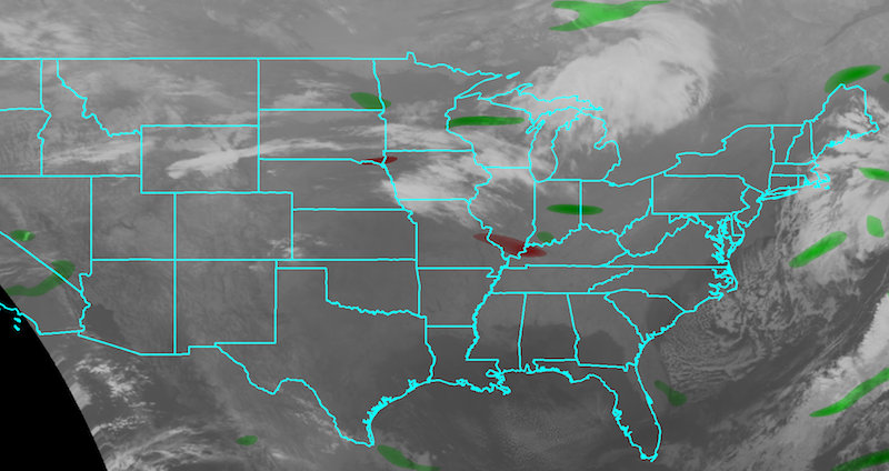
(f) 2008/09/18 13:15 GMT

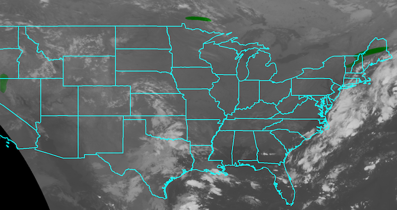
(g) 2008/03/25 12:15 GMT

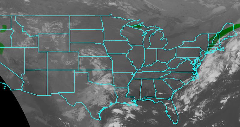
(h) 2008/03/25 12:45 GMT

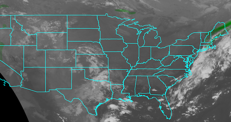
(i) 2008/03/25 13:15 GMT

Figure 6: Three example cases of applying the proposed algorithm to analyze satellite image sequences. Detected storm vortexes are colored in red and rejected vortexes are colored in green. States hit by storms are highlighted in warm colors. A red state boundary indicates the state is hit by an ongoing storm based on the historical report. As the highlighting color turns to yellow, the corresponding state is affected by more future storms as far as 6 hours away from the observation. (a-c) Three frames on May 25, 2008. Major storms occurred in the central, eastern, and southeastern states of US. Multiple vortexes are detected and classified as storm systems in each frame and the locations of the vortexes well match the ground-truth. (d-f) Image frames on September 18, 2008. The US continent area is mostly clear on the day and no vortex is detected. (g-i) Image frames on March 25, 2008. No storm is reported on the day. Though clouds and their rotational motions are perceived on the image sequence, most of them are categorized as hazardless cloud systems by the classifier.

IV Conclusions and Future Work

In this paper, we present a thunderstorm detection algorithm that locates storm visual signatures from satellite images. The algorithm automatically analyzes the visual features from satellite images and incorporates the historical meteorological records to make storm predictions. As opposed to traditional ways of weather forecasting, our approach primarily relies on the visual information from images and tries to extract high-level storm signatures as meteorologists usually do manually. Without using any sensory measurement (e.g., temperature, air pressure, etc.) as numerical weather forecasting does, the algorithm captures global cloud patterns solely from the satellite images, which is helpful in the synoptic-scale storm prediction. Additionally, the algorithm takes advantage of big data, using historical storm reports in the past years together with the satellite image archives to learn the correspondence between visual image signatures and the occurrences of current and future storms. Experiments and case studies show that the algorithm is effective and robust.

Properties of optical flows between every two images in a sequence are the basic visual clues adopted in the work. The algorithm can estimate robust and smooth optical flows between two images and determine the rotations in the flow field. Unlike numerical weather forecasting methods that are sensitive to noise and initial conditions, our approach can consistently detect reliable visual storm clues hours before the occurrence of a storm. Therefore, the results are useful for weather forecasts, especially storm forecasts.

The application of historical storm records and machine learning boosts the performance of the storm extraction algorithm. Standalone vortex detection from the optical flow is not sufficient to make reliable predictions. The statistical model trained from historical meteorological data together with the satellite image visual features further selects the extracted vortexes and removes vortexes not related to storms. In our current algorithm, storm detection is based on individual vortex regions. In reality, multiple vortexes tend to appear near each other in storm systems both temporally and geographically. Therefore, taking into account nearby vortexes within a frame and tracking storm systems across a sequence can improve the overall reliability of the system. In particular, tracking the development of a storm system will be helpful for analyzing the future trend of the storm. This problem is nontrivial because the storm systems (clouds) are non-rigid and highly variant, and the same vortexes in a storm system are not always detectable over time. Future work needs to tackle the problem of non-rigid object tracking to better make use of the temporal information in the satellite image sequences.

Lastly it should be emphasized that weather systems are highly complex and chaotic, so it is always a challenging task to make accurate weather forecasts. The proposed algorithm based on the satellite image visual features is not completely accurate and needs to be further validated. We expect the algorithm or similar approaches to play a part in producing weather forecasts rather than making the forecasts alone. It could be incorporated with other existing weather prediction techniques (e.g. NWP) and used as an automatic tool to refine the current forecasts. It is useful and valuable because it provides forecasts in a different aspect from the numerical approaches. The purpose for developing the new algorithm is not to replace the current weather forecasting models, but to produce additional independent predictions to be combined with other approaches. As a result, we will focus the future study on how to integrate information from multiple data sources and predictions from different models to produce more reliable and timely storm forecasts.

References

- [1] P. Lynch, “The origins of computer weather prediction and climate modeling,” Journal of Computational Physics, vol. 227, no. 7, pp. 3431–3444, 2008.
- [2] G. W. Platzman, “The eniac computations of 1950-gateway to numerical weather prediction,” Bulletin of the American Meteorological Society, vol. 60, no. 4, pp. 302–312, 1979.
- [3] J. Charney, “The use of the primitive equations of motion in numerical prediction,” Tellus, vol. 7, no. 1, pp. 22–26, 1955.
- [4] F. Yang, “Review of gfs forecast skills in 2013,” National Centers for Environmental Prediction, 2013.
- [5] H. W. Lean, P. A. Clark, M. Dixon, N. M. Roberts, A. Fitch, R. Forbes, and C. Halliwell, “Characteristics of high-resolution versions of the met office unified model for forecasting convection over the united kingdom,” Monthly Weather Review, vol. 136, no. 9, pp. 3408–3424, 2008.
- [6] M. Déqué et al., “Documentation arpege-climat,” CNRM (Available from Centre National de Recherches Meteorologiques, Météo-France, Toulouse, France), 1999.
- [7] P. Gauthier, C. Charette, L. Fillion, P. Koclas, and S. Laroche, “Implementation of a 3d variational data assimilation system at the canadian meteorological centre. part i: The global analysis,” Atmosphere-Ocean, vol. 37, no. 2, pp. 103–156, 1999.
- [8] S. D. Burt and D. A. Mansfield, “The great storm of 15–16 october 1987,” Weather, vol. 43, no. 3, pp. 90–110, 1988.
- [9] E. S. Blake, T. B. Kimberlain, R. J. Berg, J. Cangialosi, and J. L. Beven II, “Tropical cyclone report: Hurricane sandy,” National Hurricane Center, vol. 12, pp. 1–10, 2013.
- [10] R. L. Winkler, “The importance of communicating uncertainties in forecasts: Overestimating the risks from winter storm juno,” Risk Analysis, vol. 35, no. 3, pp. 349–353, 2015.
- [11] A. C. Lorenc and T. Payne, “4d-var and the butterfly effect: Statistical four-dimensional data assimilation for a wide range of scales,” Quarterly Journal of the Royal Meteorological Society, vol. 133, no. 624, pp. 607–614, 2007.
- [12] J. D. Doyle, C. Amerault, C. A. Reynolds, and P. A. Reinecke, “Initial condition sensitivity and predictability of a severe extratropical cyclone using a moist adjoint,” Monthly Weather Review, vol. 142, no. 1, pp. 320–342, 2014.
- [13] V. F. Dvorak, “Tropical cyclone intensity analysis and forecasting from satellite imagery,” Monthly Weather Review, vol. 103, no. 5, pp. 420–430, 1975.
- [14] R. A. Scofield, “The nesdis operational convective precipitation-estimation technique,” Monthly Weather Review, vol. 115, no. 8, pp. 1773–1793, 1987.
- [15] G. Liu, “Satellite microwave remote sensing of clouds and precipitation,” Observation, Theory and Modeling of Atmospheric Variability: Selected Papers of Nanjing Institute of Meteorology Alumni in Commemoration of Professor Jijia Zhang, vol. 3, p. 397, 2004.
- [16] A. N. Srivastava and J. Stroeve, “Onboard detection of snow, ice, clouds and other geophysical processes using kernel methods,” in Proceedings of the ICML 2003 Workshop on Machine Learning Technologies for Autonomous Space Applications, 2003.
- [17] Y. Hong, “Precipitation estimation from remotely sensed imagery using an artificial neural network cloud classification system,” Journal of Applied Meteorology, vol. 43, pp. 1834–1852, 2004.
- [18] A. Behrangi, K. Hsu, B. Imam, and S. Sorooshian, “Daytime precipitation estimation using bispectral cloud classification system,” Journal of Applied Meteorology and Climatology, vol. 49, pp. 1015–1031, 2010.
- [19] J. C. Price, “Using spatial context in satellite data to infer regional scale evapotranspiration,” IEEE Transactions on Geoscience and Remote Sensing, vol. 28, no. 5, pp. 940–948, 1990.
- [20] K. Bedka, J. Brunner, R. Dworak, W. Feltz, J. Otkin, and T. Greenwald, “Objective satellite-based detection of overshooting tops using infrared window channel brightness temperature gradients,” Journal of Applied Meteorology and Climatology, vol. 49, no. 2, pp. 181–202, 2010.
- [21] K. M. Bedka, “Overshooting cloud top detections using msg seviri infrared brightness temperatures and their relationship to severe weather over europe,” Atmospheric Research, vol. 99, no. 2, pp. 175–189, 2011.
- [22] S.-S. Ho and A. Talukder, “Automated cyclone discovery and tracking using knowledge sharing in multiple heterogeneous satellite data,” in Proceedings of the 14th ACM SIGKDD International Conference on Knowledge Discovery and Data Mining, 2008, pp. 928–936.
- [23] T. Zinner, H. Mannstein, and A. Tafferner, “Cb-tram: Tracking and monitoring severe convection from onset over rapid development to mature phase using multi-channel meteosat-8 seviri data,” Meteorology and Atmospheric Physics, vol. 101, no. 3-4, pp. 191–210, 2008.
- [24] C. Keil and G. C. Craig, “A displacement and amplitude score employing an optical flow technique,” Weather and Forecasting, vol. 24, no. 5, pp. 1297–1308, 2009.
- [25] D. Merk and T. Zinner, “Detection of convective initiation using meteosat seviri: implementation in and verification with the tracking and nowcasting algorithm cb-tram,” Atmospheric Measurement Techniques Discussions, vol. 6, pp. 1771–1813, 2013.
- [26] A. N. Evans, “Cloud motion analysis using multichannel correlation-relaxation labeling,” IEEE Geoscience and Remote Sensing Letters, vol. 3, no. 3, pp. 392–396, 2006.
- [27] A. McGovern, A. Kruger, D. Rosendahl, and K. Droegemeier, “Open problem: dynamic relational models for improved hazardous weather prediction,” in Proceedings of ICML Workshop on Open Problems in Statistical Relational Learning, vol. 29, 2006.
- [28] NOAA, “Earth location user’s guide (elug). rev. 1, noss/osd3-1998-015r1ud0,” no. NOAA/NESDIS DRL 504-11, 1998.
- [29] J. P. Snyder, Map projections–A working manual. USGPO, 1987, no. 1395.
- [30] J. Marshall and R. A. Plumb, Atmosphere, ocean and climate dynamics: an introductory text. Academic Press, 1965, vol. 8.
- [31] R. G. Barry and R. J. Chorley, Atmosphere, weather and climate. Routledge, 2009.
- [32] A. J. Clark, C. J. Schaffer, W. A. Gallus Jr, and K. Johnson-O’Mara, “Climatology of storm reports relative to upper-level jet streaks,” Weather and Forecasting, vol. 24, no. 4, pp. 1032–1051, 2009.
- [33] J. G. Charney, “The dynamics of long waves in a baroclinic westerly current,” Journal of Meteorology, vol. 4, no. 5, pp. 136–162, 1947.
- [34] T. N. Carlson, “Airflow through midlatitude cyclones and the comma cloud pattern,” Monthly Weather Review, vol. 108, no. 10, pp. 1498–1509, 1980.
- [35] J. M. Wallace and P. V. Hobbs, Atmospheric science: an introductory survey, vol. 92.
- [36] C. A. Doswell III, “Weather forecasting by humans-heuristics and decision making,” Weather and Forecasting, vol. 19, no. 6, pp. 1115–1126, 2004.
- [37] B. K. Horn and B. G. Schunck, “Determining optical flow,” in 1981 Technical Symposium East, 1981, pp. 319–331.
- [38] B. D. Lucas and T. Kanade, “An iterative image registration technique with an application to stereo vision.” in IJCAI, vol. 81, 1981, pp. 674–679.
- [39] J. S. Pérez, E. Meinhardt-Llopis, and G. Facciolo, “Tv-l1 optical flow estimation,” Image Processing On Line, vol. 2013, pp. 137–150, 2013.
- [40] J. Bouguet, “Pyramidal implementation of the affine lucas kanade feature tracker description of the algorithm,” Intel Corporation, vol. 5, 2001.
- [41] T. Acharya and A. K. Ray, Image processing: principles and applications, 2005.
- [42] R. Temam, Navier–Stokes Equations. American Mathematical Soc., 1984.
- [43] J. Stam, “Stable fluids,” in Proceedings of the 26th annual conference on Computer graphics and interactive techniques, 1999, pp. 121–128.
- [44] S. I. Green, Fluid Vortices: Fluid Mechanics and Its Applications. Springer, 1995, vol. 30.
- [45] G. B. Arfken and H. J. Weber, Mathematical Methods for Physicists, 4th ed. Academic Press: San Diego, 1995.
- [46] J. C. Hunt, A. Wray, and P. Moin, “Eddies, streams, and convergence zones in turbulent flows,” in Studying Turbulence Using Numerical Simulation Databases, 2, vol. 1, 1988, pp. 193–208.
- [47] L. Breiman, “Random forests,” Machine learning, vol. 45, no. 1, pp. 5–32, 2001.
- [48] F. Molteni, R. Buizza, T. N. Palmer, and T. Petroliagis, “The ecmwf ensemble prediction system: Methodology and validation,” Quarterly Journal of the Royal Meteorological Society, vol. 122, no. 529, pp. 73–119, 1996.