APPLICATION OF THE MAXIMUM RELATIVE ENTROPY METHOD TO THE PHYSICS OF FERROMAGNETIC MATERIALS

Abstract

It is known that the Maximum relative Entropy (MrE) method can be used to both update and approximate probability distributions functions in statistical inference problems. In this manuscript, we apply the MrE method to infer magnetic properties of ferromagnetic materials. In addition to comparing our approach to more traditional methodologies based upon the Ising model and Mean Field Theory, we also test the effectiveness of the MrE method on conventionally unexplored ferromagnetic materials with defects.

I Introduction

In 1957, Jaynes Jaynes ; Jaynes2 showed that maximizing statistical mechanic entropy for the purpose of revealing how gas molecules were distributed was simply the maximizing of the Shannon information entropy Shannon1948 with statistical mechanical information. This idea lead to MaxEnt or his use of the Method of Maximum Entropy for assigning probabilities. This method has recently evolved to a more general method, the method of Maximum relative Entropy (MrE) CatichaGiffin which has the advantage of not only assigning probabilities but updating them when new information is given in the form of constraints on the family of allowed posteriors. One of the drawbacks of the MaxEnt method was the inability to include data. When data was present, one used Bayesian methods. The methods were combined in such a way that MaxEnt was used for assigning a prior for Bayesian methods, as Bayesian methods could not deal with information in the form of constraints, such as expected values. Previously it has been shown that one can use the MrE method to reproduce a mean field solution for a simple fluid Tseng . The purpose of this was to illustrate that in addition to updating probabilities, MrE can also be used for approximating probability distributions as an approximation tool.

In a simple ferromagnetic material (that is, a ferromagnetic material with a single domain), the electronic spins of the individual atoms are strong enough to affect one and other, and give rise to the so called exchange interaction Reif . This effect, however, is temperature dependent. When the temperature is below a certain point (the Curie or critical temperature) the spins tend to all point in the same direction due to their influence on each other. This establishes a permanent magnet as the individual atoms produce a net dipole effect. Above this temperature, the atoms cease to have a significant effect on each other and the material behaves more like a paramagnetic substance. Determining this net dipole effect can be difficult. First, the interactions are due to complicated quantum effects. Second, since a given material has a very large number of atoms, computing the net dipole effect can be difficult in two dimensions and completely intractable in three dimensions. Therefore, approximations such as using an Ising Model lieb64 ; brush67 ; cipra00 and/or the mean field approximation huang ; mermin ; Schroeder are made to facilitate computation.

Applications of the MrE (updating) method together with information geometric methods used to characterize the complexity of dynamical systems described in terms of probabilistic tools are quite extensive carlo1 ; carlo2 ; carlo3 ; carlo4 ; carlo5 ; carlo6 ; carlo7 ; carlo8 ; carlo9 . In Ref. carlo2 ; carlo3 , using the MrE method together with differential geometric techniques, we proposed an information-geometric characterization of chaotic energy level statistics of a quantum antiferromagnetic Ising spin chain in a tilted magnetic field. In Ref. carlo9 , employing the very same aforementioned techniques, we were able to establish a connection between the behavior of the information-geometric complexity of a trivariate Gaussian statistical model and the geometric frustration phenomena that appears in triangular Ising models sadoc06 . However, the purpose of our article is to illustrate the use of the MrE (approximating) method as a tool for attaining approximations for ferromagnetic materials that lie outside the ability of traditional methods. In doing so, we further the previous work done and show the versatility of the method.

The layout of the remaining part of this manuscript is as follows. In Section II, we briefly outline the essential steps of the MrE method in updating and approximating probability distributions. In Section III, we describe the basics of the Ising model and Mean Field Theory as approximate mathematical descriptions of ferromagnetic materials. In Section IV, we compare magnetization properties of ferromagnets inferred by means of MrE with those obtained via the Ising model together with Mean Field Theory. In Section V, we further test the effectiveness of the MrE methodology by considering ferromagnetic material in the presence of defects. Our final remarks appear in Section VI.

II The Maximum relative Entropy method

In this Section, we outline the essential elements of the MrE method as a technique for updating and/or approximating probability distributions.

II.1 Updating probability distributions

The MrE method is a technique for updating probabilities when new information is provided in the form of a constraint on the family of the allowed posteriors. The main feature of the MrE method is the possibility of updating probabilities in the presence of both data and expected value constraints. This feature was first formally presented in CatichaGiffin where, in particular, it was shown that Bayes updating can be regarded as a special case of the MrE method. A first semi-quantitative analysis of the effective advantages of this powerful feature of the MrE method appeared in giffin-caticha . Finally, the first fully quantitative investigation of the advantages of the MrE method was carried out in giffin where two toy problems were solved in detail. Following these lines of investigation, we present here a novel application of the MrE method to a real-world ferromagnetic problem.

We use the MrE method to update from a prior to a posterior probability distribution. Specifically, we want to make inferences on some quantity $\theta\in\Theta$ given:

i)

the prior information about $\theta$ (the prior);

ii)

the known relationship between $D\in\mathcal{D}$ and $\theta\in\Theta$ (the model);

iii)

the observed values of the variables (data) $D\in\mathcal{D}$.

The search space for the posterior probability distribution occurs in the product space $\mathcal{D\times}\Theta$, and the joint distribution is denoted as $P\left(D\text{, }\theta\right)$. The key idea is going from the old prior $P_{\text{old}}\left(\theta\right)$ to the updated prior $P_{\text{new}}\left(\theta\right)$,

$$P_{\text{new}}\left(\theta\right)\overset{\text{def}}{=}\int dDP_{\text{new}}\left(D\text{, }\theta\right)\text{.}$$ (1)

The joint probability $P_{\text{new}}\left(D\text{, }\theta\right)$ maximizes the relative entropy functional $S\left[P\left|P_{\text{old}}\right.\right]$,

$$S\left[P\left|P_{\text{old}}\right.\right]\overset{\text{def}}{=}-\int dDd\theta P\left(D\text{, }\theta\right)\log\left[\frac{P\left(D\text{, }\theta\right)}{P_{\text{old}}\left(D\text{, }\theta\right)}\right]\text{,}$$ (2)

subject to the given information constraints. Note that $P_{\text{old}}\left(D\text{, }\theta\right)$,

$$P_{\text{old}}\left(D\text{, }\theta\right)=P_{\text{old}}\left(D\left|\theta\right.\right)P_{\text{old}}\left(\theta\right)\text{,}$$ (3)

is called here the joint prior, while $P_{\text{old}}\left(\theta\right)$ and $P_{\text{old}}\left(D\left|\theta\right.\right)$ denote the standard Bayesian prior and the likelihood, respectively. We emphasize that both the joint prior and the standard Bayesian prior encode prior information about $\theta\in\Theta$. Furthermore, despite the fact that the likelihood is not regarded as prior information in the conventional sense, it will be considered here as prior information since it represents the a priori established relation between $\theta\in\Theta$ and $D\in\mathcal{D}$. Let us specify now the relevant information constraints. First, we impose the standard normalization constraint,

$$\int dDd\theta P\left(D\text{, }\theta\right)=1\text{.}$$ (4)

Second, we consider an information constraint in the form of expected value of some smooth function $g\left(\theta\right)$,

$$\int dDd\theta g\left(\theta\right)P\left(D\text{, }\theta\right)\overset{\text{def}}{=}\left\langle g\left(\theta\right)\right\rangle\equiv G\text{.}$$ (5)

Finally, we consider the observed data $D^{\prime}$. Within the MrE method, knowledge of this information leads to an infinite number of constraints,

$$\int d\theta P\left(D\text{, }\theta\right)\equiv P\left(D\right)=\delta\left(D-D^{\prime}\right)\text{,}$$ (6)

for any $D\in\mathcal{D}$ where $\delta$ denotes the Dirac delta function. Using the Lagrange multipliers technique, we maximize the logarithmic relative entropy functional in Eq. (2) subject to the constraints in Eqs. (4), (5), and (6). We impose that the variation with respect to $P$ of the entropy functional $S\left[P\left|P_{\text{old}}\right.\right]$ is equal to zero,

$$\delta\left\{\begin{array}[c]{c}S\left[P\left|P_{\text{old}}\right.\right]+\alpha\left[\int dDd\theta P\left(D\text{, }\theta\right)-1\right]\\ +\beta\left[\int dDd\theta g\left(\theta\right)P\left(D\text{, }\theta\right)-G\right]\\ +\int dD\gamma\left(D\right)\left[\int d\theta P\left(D\text{, }\theta\right)-\delta\left(D-D^{\prime}\right)\right]\end{array}\right\}=0\text{.}$$ (7)

We note that Eq. (6) describes the information in the data and represents an infinite number of constraints on the family $P\left(D\text{, }\theta\right)$. For this reason, there exist one constraint and one Lagrange multiplier $\gamma\left(D\right)$ for each value of $D$. After some simple algebra of variations, Eq. (7) becomes

$$\int dDd\theta\left[-\log P\left(D\text{, }\theta\right)-1+\log P_{\text{old}}\left(D\text{, }\theta\right)+\alpha+\beta g\left(\theta\right)+\gamma\left(D\right)\right]\delta P\left(D\text{, }\theta\right)=0\text{,}$$ (8)

for any $\delta P\left(D\text{, }\theta\right)$. Therefore, from Eq. (8) we find

$$P_{\text{new}}\left(D\text{, }\theta\right)=P_{\text{old}}\left(D\text{, }\theta\right)e^{-1+\alpha+\beta g\left(\theta\right)+\gamma\left(D\right)}\text{,}$$ (9)

where the Lagrange multipliers $\alpha$, $\beta$, and $\gamma\left(D\right)$ can be formally determined by substituting Eq. (9) into Eqs. (4), (5) and (6), respectively. After some algebra, we obtain

$$P_{\text{new}}\left(D\text{, }\theta\right)=\frac{e^{\beta g\left(\theta\right)}P_{\text{old}}\left(D\text{, }\theta\right)\delta\left(D-D^{\prime}\right)}{\int d\theta e^{\beta g\left(\theta\right)}P_{\text{old}}\left(D\text{, }\theta\right)}\text{.}$$ (10)

Observe that the Lagrange multiplier $\beta$ in Eq. (10) can only be implicitly determined and depends on the observed data $D^{\prime}$. Finally, marginalizing $P_{\text{new}}\left(D\text{, }\theta\right)$ over the variable $D$, we obtain the updated prior probability distribution

$$P_{\text{new}}\left(\theta\right)\overset{\text{def}}{=}\int dDP_{\text{new}}\left(D\text{, }\theta\right)=\frac{e^{\beta g\left(\theta\right)}P_{\text{old}}\left(D^{\prime}\text{, }\theta\right)}{\int d\theta e^{\beta g\left(\theta\right)}P_{\text{old}}\left(D^{\prime}\text{, }\theta\right)}\text{.}$$ (11)

For the sake of notational simplicity, define

$$\xi\left(D^{\prime}\text{, }\beta\right)\overset{\text{def}}{=}\int d\theta e^{\beta g\left(\theta\right)}P_{\text{old}}\left(D^{\prime}\text{, }\theta\right)\text{.}$$ (12)

Finally, Eq. (11) becomes

$$P_{\text{new}}\left(\theta\right)=P_{\text{old}}\left(\theta\right)P_{\text{old}}\left(D^{\prime}\left|\theta\right.\right)\frac{e^{\beta g\left(\theta\right)}}{\xi\left(D^{\prime}\text{, }\beta\right)}\text{.}$$ (13)

Note that in the absence of constraints in the form of expected values, $\beta=0$ and Eq. (13) reduces to the standard Bayes updating relation

$$P_{\text{new}}\left(\theta\right)=\frac{P_{\text{old}}\left(\theta\right)P_{\text{old}}\left(D^{\prime}\left|\theta\right.\right)}{P_{\text{old}}\left(D^{\prime}\right)}\text{.}$$ (14)

For the sake of completeness, we point out that Eq. (14) can be obtained by combining Bayes theorem,

$$P_{\text{old}}\left(\theta\left|D\right.\right)=\frac{P_{\text{old}}\left(\theta\right)P_{\text{old}}\left(D\left|\theta\right.\right)}{P_{\text{old}}\left(D\right)}\text{,}$$ (15)

and Bayes rule,

$$P_{\text{new}}\left(\theta\right)=P_{\text{old}}\left(\theta\left|D^{\prime}\right.\right)\text{.}$$ (16)

In what follows, we shall regard the MrE method as a tool for approximating probability distributions.

II.2 Approximating probability distributions

For the sake of reasoning, assume that the microstates of a system are labeled by coordinates $x$. Furthermore, assume that the probability that the system is in a microstate within a given range $dx$ is described by the canonical distribution tseng2008 ,

$$P\left(x\right)dx=\frac{e^{-\beta\mathcal{H}\left(x\right)}}{\mathcal{Z}}dx\text{,}$$ (17)

where the function $Z$ is defined as,

$$\mathcal{Z}=\int dxe^{-\beta\mathcal{H}\left(x\right)}\overset{\text{def}}{=}e^{-\beta F}\text{.}$$ (18)

In statistical mechanical terms, the quantity $F$ in Eq. (18) denotes the Helmholtz free energy. In general, to describe a system in terms of its observables, one needs to compute expected values in terms of integrals over $P$ which, in turn, depends on the Hamiltonian $\mathcal{H}\left(x\right)$. Calculating these integrals can be quite challenging especially when the Hamiltonian exhibits nonlinear interaction terms. To make things more tractable, one can think of replacing the exact expression of $P$ with an approximate expression $P_{0}$ provided that the latter preserves the relevant information content essential for our specific inferences. More specifically, $P_{0}$ can be identified in two steps. First, identify a suitable family of trial distributions $\mathcal{F}_{P_{A}}=\left\{P_{A}\right\}$ relevant for our specific problem at hand. Second, select $P_{0}$ from $\mathcal{F}_{P_{A}}$. There is no recipe for the first step. The second step is mechanical. The distribution to be selected is the one that maximizes the entropy of $P_{A}$ relative to $P$,

$$S\left[P_{A}\left|P\right.\right]=-\int dxP_{A}\left(x\right)\log\left[\frac{P_{A}\left(x\right)}{P\left(x\right)}\right]\text{.}$$ (19)

A very convenient family of trial distributions is given by the canonical distributions with a modified Hamiltonian $\mathcal{H}_{0}\left(x\text{; }\xi\right)$ where $\xi$ are parameters that label each distribution within a family,

$$P_{0}\left(x\text{; }\xi\right)dx=\frac{e^{-\beta\mathcal{H}_{0}\left(x\text{; }\xi\right)}}{\mathcal{Z}_{0}}dx\text{,}$$ (20)

where the $\mathcal{Z}_{0}$ function is given by,

$$\mathcal{Z}_{0}\overset{\text{def}}{=}e^{-\beta F_{0}\left(\xi\right)}=\int dxe^{-\beta\mathcal{H}_{0}\left(x\text{; }\xi\right)}\text{.}$$ (21)

We underline that in Sec. II, the symbol $\theta$ is used to denote one parameter or many parameters about which one wishes to make inferences. Here, as mentioned earlier, the parameters $\xi$ are used to label a family of trial distributions that are canonical with the Hamiltonian $\mathcal{H}_{0}\left(x\text{; }\xi\right)$. Substituting Eqs. (17), (18), (20), and (21) into Eq. (19), we get

$$S\left[P_{0}\left|P\right.\right]=\beta\left(F-F_{0}\right)+\beta\left\langle\mathcal{H}_{0}-\mathcal{H}\right\rangle_{0}\text{,}$$ (22)

where,

$$\left\langle\mathcal{H}_{0}-\mathcal{H}\right\rangle_{0}\overset{\text{def}}{=}\int dxP_{0}\left(x\text{; }\xi\right)\left(\mathcal{H}_{0}-\mathcal{H}\right)\text{.}$$ (23)

Note that the symbol $\left\langle\mathcal{\cdot}\right\rangle_{0}$ in Eq. (22) denotes the average over the trial distribution $P_{0}\left(x\text{; }\xi\right)$ and the subscript $0$ is simply used to recall that $P_{0}\left(x\text{; }\xi\right)$ is canonical with the modified Hamiltonian $\mathcal{H}_{0}\left(x\text{; }\xi\right)$. Since $S\left[P_{0}\left|P\right.\right]\leq 0$, Eq. (22) implies

$$F\leq F_{0}+\left\langle\mathcal{H}_{0}-\mathcal{H}\right\rangle_{0}\text{.}$$ (24)

Loosely speaking, maximizing $S$ is equivalent to minimizing $F_{0}+\left\langle\mathcal{H}_{0}-\mathcal{H}\right\rangle_{0}$. This latter minimization procedure is also known as the Bogoliubov Variational Principle kuzemsky which, as shown here, can be regarded as a special case of the MrE method.

FERROMAGNET	SYMBOL	CRITICAL TEMPERATURE
iron	Fe	1043
cobalt	Co	1388
nickel	Ni	627
gadolinium	Gd	293
dysprosium	Dy	85

Table 1: A few ferromagnetic materials with corresponding critical temperatures in degrees Kelvin.

III Ferromagnetic materials

One of the most interesting phenomena in solid state physics is represented by ferromagnetism huang ; mermin ; Schroeder . In spite of the extensive oversimplifications required to construct a tractable mathematical model describing such a phenomena, calculations concerning ferromagnetism are among the most impressive exhibition of brute force computation achieved by theoretical physicists onsager ; yang . In what follows, we shall outline the basics of the so-called Ising model of ferromagnetic materials ising . A few ferromagnetic materials together with their corresponding critical temperatures are listed in Table I.

III.1 The Ising Model

One of the simplest systems that exhibits a transition from ordered to disordered states is that of a lattice composed of two different types of objects, $A$ and $B$. Assume that the objects interact with only their nearest neighbors. If one raises the temperature $T$ of the system at some critical point $T_{c}$, the system will melt and become completely disordered. A relatively simple mathematical model of such a system was developed by Ernst Ising to describe ferromagnetism ising . The general expression for the Ising Hamiltonian is given by huang ,

$$\mathcal{H}\left\{s_{i}\right\}\overset{\text{def}}{=}-\sum_{\left\langle ij\right\rangle}J_{ij}s_{i}s_{j}-B\sum_{i=1}^{N}s_{i}\text{,}$$ (25)

where $s_{i}\in\left\{+1\text{, }-1\right\}$ is the spin variable, $N$ is the cardinality of the spin variables, $\left\{s_{i}\right\}$ determines the spin configuration of the whole system, the symbol $\left\langle ij\right\rangle$ with $\left\langle ij\right\rangle=\left\langle ji\right\rangle$ denotes a pair of next neighbor spins, $J_{ij}$ are the exchange coupling constants, and $B$ is the $z$-component of a uniform external magnetic field. Ferromagnetic and antiferromagnetic materials are characterized by exchange coupling coefficients with $J_{ij}>0$ and $J_{ij}<0$, respectively, for all pairs $i$, $j$. For instance, iron (Fe) and iron oxide (FeO) are examples of ferromagnetic and antiferromagnetic materials, respectively. Their critical temperature is given by $T_{c}^{\left(Fe\right)}=1043K$ and $T_{c}^{\left(FeO\right)}=198K$ mermin , respectively.

For the sake of reasoning, we shall assume in what follows that $B=0$ (zero external magnetic field) and $J_{ij}=J>0$ for all pairs $i$, $j$ (isotropic interaction strength). The Hamiltonian in Eq. (25) becomes,

$$\mathcal{H}\left\{s_{i}\right\}\overset{\text{def}}{=}-J\sum_{\left\langle ij\right\rangle}s_{i}s_{j}\text{.}$$ (26)

The sum over $\left\langle ij\right\rangle$ in Eq. (26) contains $\gamma N/2$ terms where $\gamma$ is the number of next nearest neighbors of each lattice site and depends on the specific type of lattice structure being considered. For instance, for a two-dimensional square lattice, $\gamma=4$. The partition function $\mathcal{Z}\left(T\right)$ corresponding to the Hamiltonian in Eq. (26) is the sum of $2^{N}$ terms and is given by huang ,

$$\mathcal{Z}\left(T\right)\overset{\text{def}}{=}\sum_{s_{1}}\sum_{s_{2}}\text{...}\sum_{s_{N}}e^{-\beta\mathcal{H}\left\{s_{i}\right\}}\text{,}$$ (27)

where $\beta=\beta\left(k_{B}\text{, }T\right)\overset{\text{def}}{=}\left(k_{B}T\right)^{-1}$, with $k_{B}\approx 1.38\times 10^{-23}JK^{-1}$ denoting the Boltzmann constant. As a side remark, we recall that the thermodynamic functions (internal energy and thermal capacity, for instance) can be obtained in the usual manner from the Helmholtz free energy $F\left(T\right)$ huang ,

$$F\left(T\right)\overset{\text{def}}{=}-k_{B}T\log\mathcal{Z}\left(T\right)\text{.}$$ (28)

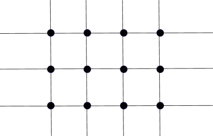
Figure 1: Schematic illustration of a rectangular two-dimensional Ising model.

In the two-dimensional case with only nearest neighbor interactions and simple lattice configurations (square and triangular, for instance), the exact free energy is known in the hypothesis of zero magnetic field onsager ; yang . For the one dimensional case, the partition function $\mathcal{Z}\left(T\right)$ can easily be calculated,

$$\mathcal{Z}\left(T\right)=2^{N}\left[\cosh\left(\beta J\right)\right]^{N-1}\overset{N\gg 1}{\approx}\left[2\cosh\left(\beta J\right)\right]^{N}\text{.}$$ (29)

Furthermore, the resulting average energy $\mathcal{\bar{H}}$ for $N\gg 1$ would then be,

$$\mathcal{\bar{H}}=-\frac{\partial\log Z}{\partial\beta}=-NJ\tanh\left(\beta J\right)~{}\text{,}$$ (30)

where $\tanh\left(\cdot\right)$ denotes the hyperbolic tangent function. For the sake of clarity, a rectangular two-dimensional Ising model is depicted in FIG. 1.

III.2 The mean field approximation

One of the most important starting points for more sophisticated calculations concerning ferromagnetic transitions is furnished by the so-called mean field theory (or, molecular field theory weiss ). The mean field approximation for the Ising model assumes that each and every spin is subject to a mean field generated by its next nearest neighbors only huang . Such an approximation turns out to be especially important for three dimensional materials where each atom may have $6$, $8$ or even $12$ close neighbors depending on the crystal geometry Reif ; Schroeder .

We start with the same energy function as given in Eq. (26) but now examine only one atom (sometimes called the central atom),

$$\mathcal{H}_{i}=-Js_{i}\sum_{j=1}^{n}s_{j}~{}\text{,}$$ (31)

where $\mathcal{H}_{i}$ is the energy ascribed to one atom and $n$ is the number of nearest neighbors (for instance, a face-centered cubic lattice would have $n=12$) with atoms at the edge of the material neglected. Assuming that each neighbor contributes equally and averaging over the neighbor spins around this one atom, we obtain

$$\mathcal{\bar{H}}_{i}=-Js_{i}n\bar{s}_{j}\text{,}$$ (32)

where,

$$\bar{s}_{j}\overset{\text{def}}{=}\frac{1}{n}\sum_{j=1}^{n}s_{j}\text{,}$$ (33)

with $j\in\left\{1\text{,..., }n\right\}$. The Boltzmann probability $p_{i}$ of finding this atom in the $s_{i}$ state is given by,

$$p_{i}=\frac{1}{\mathcal{Z}_{i}}e^{-\beta\mathcal{\bar{H}}_{i}}\text{, }$$ (34)

and the partition function $\mathcal{Z}_{i}$ becomes,

$$\mathcal{Z}_{i}=2\cosh\left(\beta Jn\bar{s}_{j}\right)\text{.}$$ (35)

Taking the average of $s_{i}$ for this one atom over its two possible states, using Eqs. (34) and (35), the mean magnetization becomes

$$\left\langle s_{i}\right\rangle\overset{\text{def}}{=}\sum_{s_{i}}s_{i}~{}p_{i}=\frac{1}{\mathcal{Z}_{i}}\left[(1)e^{\beta\mathcal{\bar{H}}_{i}}+(-1)e^{-\beta\mathcal{\bar{H}}_{i}}\right]=\frac{2\sinh\left(\beta Jn\bar{s}_{j}\right)}{2\cosh\left(\beta Jn\bar{s}_{j}\right)}=\tanh\left(\beta Jn\bar{s}_{j}\right)~{}\text{.}$$ (36)

Furthermore, assuming that all atoms will behave like this one labeled with the $i$ index and assuming that the average spin $\bar{s}$ for the entire ferromagnetic material is formally defined as,

$$\bar{s}\overset{\text{def}}{=}\left\langle\left\langle s_{i}\right\rangle\right\rangle=\left\langle\bar{s}_{j}\right\rangle\text{,}$$ (37)

from Eqs. (36) and (37), we find

$$\bar{s}=\tanh\left(\beta Jn\bar{s}\right)\text{.}$$ (38)

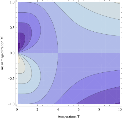
Figure 2: Contour plot exhibiting the numerical solution of the mean magnetization $M$ vs. temperature $T$ in case of the mean field approximation applied to the Ising model. We set $k_{B}=1$ and assume $n=4$, $J=1$, and the level curves $f\left(M\text{, }T\right)=c$ with $c\in\left\{-0.8\text{, }-0.6\text{,..., }0\text{, }0.2\text{,..., }0.6\right\}.$

Observe that the inner and outer expectation values in the nested expectation value in Eq. (37) used to define the average spin $\bar{s}$ for the entire ferromagnetic material represent the averages over all possible states of an atom and over all atoms of the material, respectively. If one considers Eq. (25) instead of Eq. (26), Eq. (38) can be generalized and becomes mac ,

$$\bar{s}=\tanh\left[\beta\left(nJ\bar{s}+B\right)\right]\text{,}$$ (39)

where $B$ denotes the intensity of the applied external magnetic field. Eq. (39) can be solved numerically in order to uncover the mean magnetization $M\overset{\text{def}}{=}\bar{s}$ as a function of the temperature $T$ of the system. A contour plot of $f\left(M\text{, }T\right)$ defined as,

$$f\left(M\text{, }T\right)\overset{\text{def}}{=}M-\tanh\left[\frac{1}{k_{B}T}\left(nJM+B\right)\right]\text{,}$$ (40)

as a function of $M$ and $T$ appears in FIG. 2. When an external magnetic field with strength $B$ is applied, the effective Hamiltonian $\left(\mathcal{\bar{H}}_{i}\right)_{\text{eff}}$ for the $i$-th atom becomes,

$$\left(\mathcal{\bar{H}}_{i}\right)_{\text{eff}}=-Js_{i}n\bar{s}_{j}~{}-\mu Bs_{i}=-\epsilon s_{i}\text{,}$$ (41)

where $\mu\overset{\text{def}}{=}\frac{\epsilon}{B}$ is the magnetic moment and $\epsilon\overset{\text{def}}{=}\mu B$ is the net effective energy on the $i$-th atom. As a final remark, we also point out that if one were to write the full Hamiltonian with the external field instead of $\mathcal{H}\left\{s_{i}\right\}$ as given in Eq. (26), then one will not have as simple of a solution for $\mathcal{Z}$ as in Eq. (29), i.e. $\mathcal{Z}_{\text{eff}}\neq\left[2\cosh\left(\beta\epsilon\right)\right]^{N}$.

IV Maximum relative Entropy method and ferromagnetic materials

As we have seen in the previous Section, the Ising model and mean field theory require various assumptions to be fulfilled. Part of the strength of using the MrE is that one does not need to justify some of the assumptions. Stated otherwise, one simply supplies the information constraints that one has available and then allow the method to turn out the least biased solution based on the information given. This can be demonstrated by using the MrE method to find an appropriate approximate description of a ferromagnetic material.

Following the procedure outlined in Section II, we begin by determining the full posterior solution for a ferromagnetic atomic system where we have both an expectation value constraint as well as observed data. For this example, the data observed will be the effect of the external magnetic field, $B_{i}$ on each atom. The appropriate entropy to consider becomes,

$$S[p|p_{\text{old}}]=-\int d^{N}B\sum_{\left\{s\right\}}p\left\{s,B\right\}\log\left[\frac{p\left\{s,B\right\}}{p_{\text{old}}\left\{s,B\right\}}\right]$$ (42)

where $p\left\{s,B\right\}=p(s_{1},B_{1},$…$,s_{N},B_{N})$, $p_{\text{old}}\left\{s,B\right\}$ will be a flat prior (constant in $s$ and uniform in $B$), $N$ denotes the number of atoms, and

$$\int d^{N}B\sum_{\left\{s\right\}}=\int dB_{1}\ldots dB_{N}\sum_{s_{1}}\sum_{s_{2}}\text{...}\sum_{s_{N}}\text{.}$$ (43)

Second, we consider the energy constraint in the form of the expectation value of the Hamiltonian,

$$\int d^{N}B\sum_{\left\{s\right\}}\mathcal{H}\left\{s\right\}p\left\{s,B\right\}\equiv\left\langle\mathcal{H}\left\{s\right\}\right\rangle\text{ ,}$$ (44)

where $\mathcal{H}\left\{s\right\}$ denotes some general Hamiltonian. For illustrative purposes, we adopt as our starting point the Ising model so as to show how one can use the MrE to arrive at a similar approximation as the one produced by mean field theory. Let $\mathcal{H}\left\{s\right\}$ in Eq. (44) be defined as,

$$\mathcal{H}\left\{s\right\}\overset{\text{def}}{=}\mathcal{H}_{int}+\mathcal{H}_{ext}=-J\sum_{\left\langle ij\right\rangle}s_{i}s_{j}-\sum_{i=1}^{N}\mu B_{i}s_{i}\text{.}$$ (45)

where $\mathcal{H}_{int}$ equals $\mathcal{H}$ in Eq. (26) and $\mathcal{H}_{ext}$ is the energy attributed to the observed external magnetic field $B_{i}$ acting on the individual atoms. Next is to apply the data constraints. As mentioned in Section II, there are an infinite number of data constraints associated with a single data point. Therefore, here we have $N$ sets of them, one set for each data point. For illustrative purposes, we will assume that the field is uniform and therefore the value $B_{i}=B_{j}=B$ for all $i$, $j\in\left\{1\text{,..., }N\right\}$. We can then simply write the data constraint as,

$$\int dB\sum_{\left\{s\right\}}p\left\{s,B\right\}\equiv p\left\{B\right\}=\delta\left(B-B^{\prime}\right)\text{.}$$ (46)

Along with the normalization constraint, maximizing the logarithmic relative entropy with respect to the constraints yields the canonical distribution,

$$p\left\{s\right\}=\frac{1}{\mathcal{Z}^{\prime}}e^{-\beta\mathcal{H}^{\prime}\left\{s\right\}}\text{,}$$ (47)

where $p\left\{s\right\}=p(s_{1}$…$s_{N})$, $\mathcal{Z}^{\prime}$ is similar to the partition function from Eq. (27) with the exception of the data in the Hamiltonian $\mathcal{H}^{\prime}\left\{s\right\}$ which is now,

$$\mathcal{H}^{\prime}\left\{s\right\}\overset{\text{def}}{=}\mathcal{H}_{int}+\mathcal{H}_{ext}^{\prime}=-J\sum_{\left\langle ij\right\rangle}s_{i}s_{j}-\sum_{i=1}^{N}\mu B^{\prime}s_{i}\text{.}$$ (48)

However, in order to determine the values of quantities such as the critical temperature, the total magnetic moment and the magnetic susceptibility, we are faced with the same dilemma as above: we cannot compute the solutions explicitly. Therefore, we must try to find an approximation that is computationally tractable. We now wish to use MrE to find an approximation that is tractable. We accomplish this by first writing down the appropriate entropy functional $S[p_{\text{A}}|p]$,

$$S[p_{\text{A}}|p]=-\sum_{\left\{s\right\}}p_{\text{A}}\log\left[\frac{p_{\text{A}}}{p}\right]\text{,}$$ (49)

where $p$ is the canonical probability distribution as in Eq. (47) with $\mathcal{H}^{\prime}\left\{s\right\}$ as given in Eq. (48) and $p_{\text{A}}$ is the approximation that we seek. We proceed by rewriting the entropy functional $S[p_{\text{A}}|p]$ as,

$$S[p_{\text{A}}|p]=-\sum_{\left\{s\right\}}p_{\text{A}}\log p_{\text{A}}+\sum_{\left\{s\right\}}p_{\text{A}}\log p\text{.}$$ (50)

Using Eqs. (47) and (48), Eq. (50) becomes

$$S[p_{\text{A}}|p]=\frac{1}{k_{B}}S_{\text{A}}-\sum_{\left\{s\right\}}p_{\text{A}}\beta\mathcal{H}^{\prime}\left\{s\right\}+\beta F\text{,}$$ (51)

where we have used the fact that the partition function $\mathcal{Z}^{\prime}$ can also be written in terms of the free energy $F$ as $\mathcal{Z}^{\prime}=e^{-\beta F}$. Eq. (51) can further be reduced to

$$S[p_{\text{A}}|p]=\frac{1}{k_{B}}S_{\text{A}}+\beta\left(F-\left\langle\mathcal{H}^{\prime}\left\{s\right\}\right\rangle_{\text{A}}\right)\text{,}$$ (52)

where $\left\langle\mathcal{H}^{\prime}\left\{s\right\}\right\rangle_{\text{A}}$ can be regarded as the energy $E_{\text{A}}$ of the system and is formally defined as,

$$E_{\text{A}}=\left\langle\mathcal{H}^{\prime}\left\{s\right\}\right\rangle_{\text{A}}\overset{\text{def}}{=}\sum_{\left\{s\right\}}p_{\text{A}}\mathcal{H}^{\prime}\left\{s\right\}\text{.}$$ (53)

Since by definition $S[p_{\text{A}}|p]\leq 0$, using Eqs. (52) and (53) leads to

$$F\leq E_{\text{A}}-TS_{\text{A}}\text{.}$$ (54)

When using the MrE method, we maximize the entropy functional in order to find the best posterior given the information provided. For this specific case, we have rewritten the entropy in terms of an inequality that compares the free energy of the system $F$ with the approximate values for the average energy $E_{\text{A}}$ and the entropy $S_{\text{A}}$. The free energy is minimized to determine the best approximation for $p_{\text{A}}$. This minimization problem is also known as the Bogoliubov Variational Principle Tseng . Therefore, from our discussion, we conclude that this Variational Principle is simply a special case of the MrE method. To be more general, we proceed with using the MrE method to find the best approximation. As stated earlier, when using the MrE method, the goal is to search the family of possible posteriors in order to find the one that maximizes the entropy given the constraints. In addition to this, we need a solution that is tractable. Therefore, we seek a posterior $p_{\text{A}}$ that has a form

$$p_{\text{A}}=\frac{1}{\mathcal{Z}_{\text{A}}}e^{-\beta\mathcal{H}_{\text{A}}}~{}\text{,}$$ (55)

where $\mathcal{H}_{\text{A}}$ is defined as,

$$\mathcal{H}_{\text{A}}\overset{\text{def}}{=}-\sum_{i}\epsilon_{i\text{A}}s_{i}\text{,}$$ (56)

and $\epsilon_{i\text{A}}$ is some effective energy similar to $\left(\mathcal{\bar{H}}_{i}\right)_{\text{eff}}$ given in Eq. (41). For illustrative purposes, we assume that all atoms poses the same effective energy so that $\epsilon_{i\text{A}}=\epsilon_{\text{A}}$ for any $i\in\left\{1\text{,..., }N\right\}$. The difference is that we do not yet know the form of $\epsilon_{\text{A}}$. We continue by following a similar route to Eq. (36) by writing the expectation value for $s_{i}$ with respect to $p_{\text{A}}$,

$$\left\langle s_{i}\right\rangle_{\text{A}}=\sum_{\left\{s_{i}\right\}}s_{i}~{}p_{\text{A}}=\tanh\left(\beta\epsilon_{i\text{A}}\right)=\tanh\left(\beta\epsilon_{\text{A}}\right)~{}\text{,}$$ (57)

except that here we are marginalizing over all atoms except the $i$-th. Notice that because the effective energy $\epsilon_{\text{A}}$ is constant, the solution is independent of the index $i$. Next we maximize $S[p_{\text{A}}|p]$ in Eq. (49) or, in keeping with the current case, we minimize the free energy $F$. From Eq. (52), we have

$$\beta F_{\min}=-\frac{1}{k_{B}}S_{\text{A}}+\beta\left\langle\mathcal{H}^{\prime}\left\{s\right\}\right\rangle_{\text{A}}\text{.}$$ (58)

Substituting Eq. (55) into Eq. (58), after some algebra we get

$$F_{\min}=\left(\frac{1}{\beta}\sum_{\left\{s\right\}}p_{\text{A}}\log e^{-\beta\mathcal{H}_{\text{A}}}-\frac{1}{\beta}\sum_{\left\{s\right\}}p_{\text{A}}\log\mathcal{Z}_{\text{A}}\right)+\sum_{\left\{s\right\}}p_{\text{A}}\mathcal{H}^{\prime}\left\{s\right\}~{}\text{.}$$ (59)

Note that $\mathcal{Z}_{\text{A}}$ is a constant and can be extracted from the summation in Eq. (59). Furthermore, since $\sum_{\left\{s\right\}}p_{\text{A}}=1$, Eq. (59) becomes

$$F_{\min}=\left(-\frac{1}{\beta}\sum_{\left\{s\right\}}p_{\text{A}}\beta\mathcal{H}_{\text{A}}-\frac{1}{\beta}\log\mathcal{Z}_{\text{A}}\right)+\sum_{\left\{s\right\}}p_{\text{A}}\mathcal{H}^{\prime}\left\{s\right\}\text{,}$$ (60)

or expressed otherwise,

$$F_{\min}=-\left\langle\mathcal{H}_{\text{A}}\right\rangle_{\text{A}}-\frac{1}{\beta}\log\mathcal{Z}_{\text{A}}+\left\langle\mathcal{H}^{\prime}\left\{s\right\}\right\rangle_{\text{A}}~{}\text{.}$$ (61)

We now substitute the explicit expressions for the Hamiltonians $\mathcal{H}^{\prime}\left\{s\right\}$ in Eq. (48) and $\mathcal{H}_{\text{A}}$ in Eq. (56) into the function $F_{\min}$ in Eq. (61). After some algebra,  we find

$$F_{\min}=-\left\langle-\epsilon_{\text{A}}\sum_{i}s_{i}\right\rangle_{\text{A}}-\frac{1}{\beta}\log\mathcal{Z}_{\text{A}}+\left\langle-J\sum_{i,j}^{N,n}s_{i}s_{j}-\sum_{i}^{N}\mu B^{\prime}s_{i}\right\rangle_{\text{A}}~{}\text{.}$$ (62)

Noting that,

$$\left\langle\sum_{i}s_{i}\right\rangle_{\text{A}}=\sum_{i}\left\langle s_{i}\right\rangle_{\text{A}}=N\left\langle s_{i}\right\rangle_{\text{A}}=N\tanh\left(\beta\epsilon_{\text{A}}\right)\text{,}$$ (63)

$F_{\min}$  becomes,

$$F_{\min}=\epsilon_{\text{A}}N\tanh\left(\beta\epsilon_{\text{A}}\right)-\frac{1}{\beta}\log\mathcal{Z}_{\text{A}}-J\sum_{i,j}^{N,n}\left\langle s_{i}s_{j}\right\rangle_{\text{A}}-\mu B^{\prime}N\tanh\left(\beta\epsilon_{\text{A}}\right)~{}\text{.}$$ (64)

Substituting $\mathcal{Z}_{\text{A}}\overset{N\gg 1}{\approx}\left[2\cosh\left(\beta\epsilon_{\text{A}}\right)\right]^{N}$ into Eq. (64) yields,

$$F_{\min}=\epsilon_{\text{A}}N\tanh\left(\beta\epsilon_{\text{A}}\right)-\frac{1}{\beta}\log\left[2\cosh\left(\beta\epsilon_{\text{A}}\right)\right]^{N}-J\sum_{i,j}^{N,n}\left\langle s_{i}s_{j}\right\rangle_{\text{A}}-\mu B^{\prime}N\tanh\left(\beta\epsilon_{\text{A}}\right)\text{.}$$ (65)

From Eq. (57), $\left\langle s_{i}\right\rangle_{\text{A}}=\tanh\left(\beta\epsilon_{\text{A}}\right)$ and does not depend on the index $i$, so that

$$\left\langle s_{i}\right\rangle_{\text{A}}=\left\langle s_{j}\right\rangle_{\text{A}}\text{, and }\left\langle s_{i}s_{j}\right\rangle_{\text{A}}=\left\langle s_{i}\right\rangle_{\text{A}}\left\langle s_{j}\right\rangle_{\text{A}}\text{.}$$ (66)

Therefore, $F_{\min}$ can be rewritten as

$$F_{\min}=\epsilon_{\text{A}}N\tanh\left(\beta\epsilon_{\text{A}}\right)-\frac{1}{\beta}N\log\left[2\cosh\left(\beta\epsilon_{\text{A}}\right)\right]-J\sum_{i,j}^{N,n}\left\langle s_{i}\right\rangle_{\text{A}}\left\langle s_{j}\right\rangle_{\text{A}}-\mu B^{\prime}N\tanh\left(\beta\epsilon_{\text{A}}\right)~{}\text{.}$$ (67)

Substituting Eq. (57) into Eq. (67) yields,

$$F_{\min}=\epsilon_{\text{A}}N\tanh\left(\beta\epsilon_{\text{A}}\right)-\frac{N}{\beta}\log\left[2\cosh\left(\beta\epsilon_{\text{A}}\right)\right]-J\frac{1}{2}Nn\left[\tanh\left(\beta\epsilon_{\text{A}}\right)\right]^{2}-\mu B^{\prime}N\tanh\left(\beta\epsilon_{\text{A~{}}}\right)\text{,}$$ (68)

where the factor $n$ specifies the number of nearest neighbors, the factor $N$ is from the total number of atoms and the $1/2$ appears in order to take into account double counting. We now minimize $F_{\min}$ in Eq. (68) with respect to $\epsilon_{\text{A}}$,

$$\frac{\partial F_{\min}}{\partial\epsilon_{\text{A}}} =0=N\tanh\left(\beta\epsilon_{\text{A}}\right)+N\epsilon_{\text{A}}\frac{\beta}{\cosh^{2}\left(\beta\epsilon_{\text{A}}\right)}-\frac{N}{\beta}\frac{\beta\sinh\left(\beta\epsilon_{\text{A}}\right)}{\cosh\left(\beta\epsilon_{\text{A}}\right)}+$$

$$-J\frac{1}{2}Nn2\tanh\left(\beta\epsilon_{\text{A}}\right)\frac{\beta}{\cosh^{2}\left(\beta\epsilon_{\text{A}}\right)}-\mu B^{\prime}N\frac{\beta}{\cosh^{2}\left(\beta\epsilon_{\text{A}}\right)}~{}\text{,}$$ (69)

that is,

$$0 =N\tanh\left(\beta\epsilon_{\text{A}}\right)+N\epsilon_{\text{A}}\frac{\beta}{\cosh^{2}\left(\beta\epsilon_{\text{A}}\right)}-N\tanh\left(\beta\epsilon_{\text{A}}\right)+$$

$$-JNn\tanh\left(\beta\epsilon_{\text{A}}\right)\frac{\beta}{\cosh^{2}\left(\beta\epsilon_{\text{A}}\right)}-\mu B^{\prime}N\frac{\beta}{\cosh^{2}\left(\beta\epsilon_{\text{A}}\right)}~{}\text{.}$$ (70)

After canceling terms in Eq. (70), we have

$$0=\epsilon_{\text{A}}-\mu B^{\prime}-Jn\tanh\beta\epsilon_{\text{A}}$$ (71)

that is,

$$\epsilon_{\text{A}}-\mu B^{\prime}=Jn\tanh\left(\beta\epsilon_{\text{A}}\right)~{}\text{.}$$ (72)

Eq. (72) is our final result for this Section. In FIG. 2, the numerical solution of the mean magnetization vs. temperature is reported. We note that for $T=T_{c}=4$ and $h=0$,

$$\lim_{T\rightarrow T_{c}}\left|\frac{dM\left(T\right)}{dT}\right|=\infty\text{.}$$ (73)

The critical temperature $T_{c}$ is the temperature at which spontaneous magnetization in a lattice of magnetic material begins to appear, and this is where a phase transition occurs stanleybook . Roughly speaking, a phase transition in a lattice is a singularity in the limit of $\frac{\log Z\left(T\right)}{D}$ as $D$, the size of the lattice, approaches infinity. For the sake of completeness, we remark here that while Onsager was the first to obtain a closed-form solution to the Ising two-dimensional ferromagnetic model in the absence of an external magnetic field onsager , Yang was the first to publish the exact calculation of the spontaneous magnetization for a two-dimensional Ising model yang . Returning to FIG. 2, we note that for $T>T_{c}$, there is only one approximating probability distribution that is uniform over all states. For $T<T_{c}$, there are two minima that correspond to approximating distributions that are symmetry-broken, with all spins more likely to be down, or all spins more likely to be up. Furthermore, notice that if $B^{\prime}=0$ in Eq. (72), we recover our solution using the mean field approximation above. As a matter of fact, letting $\epsilon_{\text{A}}=Jn\bar{s}$, we rewrite Eq. (72) as,

$$Jn\bar{s}=Jn\tanh\left(\beta Jn\bar{s}\right)~{}\text{,}$$ (74)

that is, we reattain Eq. (38),

$$\bar{s}=\tanh\left(\beta Jn\bar{s}\right)~{}\text{.}$$ (75)

However, from Eq. (72) alone we can formally solve for the critical temperature, the total magnetic moment and the magnetic susceptibility (that is, the ratio between the magnetization of the material and the strength of the magnetic field applied to the material) in the usual way Caticha . This is true even though we still do not know the explicit form for $\epsilon_{\text{A}}$. Using this MrE approach, we did not need to assume that all atoms behave like a central atom and we did not need to know the explicit form of the effective energy $\epsilon_{\text{A}}$, only that there was one. Following the MrE method we simply processed all of the information that we had available. Notice that we also no longer need to assume Ising conditions. We further explore such considerations in the next Section.

V Example toy applications

In this Section, we employ MrE techniques to infer the numerical estimates of effective energy levels of atoms in two cases: i) atoms with three possible states; ii) defective atoms in a crystal lattice.

V.1 Atoms with three possible states

To illustrate the use of MrE in determining critical temperatures, we look at the Ising model with three possible states: spin up, spin down, and no spin. In this example, we will let $s\in\{+1,0,-1\}$ where an atom in the $0$-state would contribute no energy. We follow the same line of reasoning outlined in the previous Section up until Eq. (57) where the new expected value for the $i$-th spin variable $\left\langle s_{i}\right\rangle_{\text{A}}$ is now given by,

$$\left\langle s_{i}\right\rangle_{\text{A}}\overset{\text{def}}{=}\sum_{\left\{s_{i}\right\}}s_{i}~{}p_{\text{A}}=\frac{2\sinh\left(\beta\epsilon_{\text{A}}\right)}{2\cosh\left(\beta\epsilon_{\text{A}}\right)+1}\text{~{}.}$$ (76)

After some tedious algebra, the new expression for $F_{\min}$ becomes

$$F_{\min}=\epsilon_{\text{A}}N\frac{2\sinh\left(\beta\epsilon_{\text{A}}\right)}{2\cosh\left(\beta\epsilon_{\text{A}}\right)+1}-\frac{N}{\beta}\log\left[2\cosh\left(\beta\epsilon_{\text{A}}\right)+1\right]-J\frac{1}{2}Nn\left[\frac{2\sinh\left(\beta\epsilon_{\text{A}}\right)}{2\cosh\left(\beta\epsilon_{\text{A}}\right)+1}\right]^{2}-\mu B^{\prime}N\frac{2\sinh\left(\beta\epsilon_{\text{A}}\right)}{2\cosh\left(\beta\epsilon_{\text{A}}\right)+1}~{}\text{.}$$ (77)

Minimizing this function $F_{\min}$ once again with respect to $\epsilon_{\text{A}}$ yields,

$$\left.\frac{\partial F_{\min}}{\partial\epsilon_{\text{A}}}\right|_{\epsilon_{\text{A}}=~{}\epsilon_{\text{A}\min}} =0=N\frac{2\sinh\left(\beta\epsilon_{\text{A}}\right)}{2\cosh\left(\beta\epsilon_{\text{A}}\right)+1}+N\epsilon_{\text{A}}\left(\frac{2\beta\cosh\left(\beta\epsilon_{\text{A}}\right)}{2\cosh\left(\beta\epsilon_{\text{A}}\right)+1}-\frac{4\beta\sinh^{2}\left(\beta\epsilon_{\text{A}}\right)}{\left[2\cosh\left(\beta\epsilon_{\text{A}}\right)+1\right]^{2}}\right)+$$

$$-\frac{N}{\beta}\frac{2\beta\sinh\left(\beta\epsilon_{\text{A}}\right)}{2\cosh\left(\beta\epsilon_{\text{A}}\right)+1}-J\frac{1}{2}Nn2\left(\frac{2\sinh\left(\beta\epsilon_{\text{A}}\right)}{2\cosh\left(\beta\epsilon_{\text{A}}\right)+1}\right)\left(\frac{2\beta\cosh\left(\beta\epsilon_{\text{A}}\right)}{2\cosh\left(\beta\epsilon_{\text{A}}\right)+1}-\frac{4\beta\sinh^{2}\left(\beta\epsilon_{\text{A}}\right)}{\left[2\cosh\left(\beta\epsilon_{\text{A}}\right)+1\right]^{2}}\right)+$$

$$-\mu B^{\prime}N\left(\frac{2\beta\cosh\left(\beta\epsilon_{\text{A}}\right)}{2\cosh\left(\beta\epsilon_{\text{A}}\right)+1}-\frac{4\beta\sinh^{2}\left(\beta\epsilon_{\text{A}}\right)}{\left[2\cosh\left(\beta\epsilon_{\text{A}}\right)+1\right]^{2}}\right)~{}\text{.}$$ (78)

After canceling terms in Eq. (78), we arrive at

$$\epsilon_{\text{A}}-\mu B^{\prime}=Jn\left(\frac{2\sinh\left(\beta\epsilon_{\text{A}}\right)}{2\cosh\left(\beta\epsilon_{\text{A}}\right)+1}\right)\text{.}$$ (79)

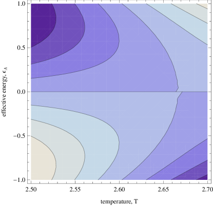
Figure 3: Contour plot exhibiting the numerical solution of the effective energy $\epsilon_{A}$ vs. temperature $T$. We set $k_{B}=1$ and assume $n=4$, $J=1$, $\mu=1$, $B^{\prime}=1$ and the level curves $f\left(\epsilon_{A}\text{, }T\right)=c$ with $c\in\left\{-1.03\text{, }-1.02\text{, }-1.01\text{, }-1\text{, }-0.99\text{, }-0.98\text{, }-0.97\right\}$.

Eq. (79) is our final result. A contour plot of $f\left(\epsilon_{\text{A}}\text{, }T\right)$ defined as,

$$f\left(\epsilon_{\text{A}}\text{, }T\right)\overset{\text{def}}{=}\epsilon_{\text{A}}-\mu B^{\prime}-Jn\left(\frac{2\sinh\left(\frac{\epsilon_{\text{A}}}{k_{B}T}\right)}{2\cosh\left(\frac{\epsilon_{\text{A}}}{k_{B}T}\right)+1}\right)\text{,}$$ (80)

as a function of $\epsilon_{\text{A}}$ and $T$ appears in FIG. 3. As stated earlier, this equation can then be used as above to solve for the critical temperature, the total magnetic moment and the magnetic susceptibility for this specific ferromagnetic material. As a side remark, we note that to make this result a little more general we can also write,

$$\epsilon_{\text{A}}-\mu B^{\prime}=Jn_{\text{G}}\left(-\frac{\partial\ln\mathcal{Z}_{\text{A}}}{\partial\epsilon_{\text{A}}}\right)=Jn_{\text{G}}\beta\left(\frac{\partial F_{\text{A}}}{\partial\epsilon_{\text{A}}}\right)=Jn_{\text{G}}\left(\left\langle s_{i}\right\rangle_{\text{A}}\right)~{}\text{,}$$ (81)

where $\mathcal{Z}_{\text{A}}$ is once again the approximate partition function, $n_{\text{G}}$ is the number of nearest neighbors and $F_{\text{A}}$ is the approximate free energy. Despite its lack of elegance, our entropic analysis leading to Eq. (79) together with FIG. 3 seems to support the idea that the introduction of additional (allowed) states in the atomic ferromagnetic structure is consistent with both space shifts and nonhomogeneities of the critical temperature jean00 ; kallin08 . A deeper understanding of these specific aspects require a deeper analysis that we leave to future investigations.

As a side remark, although unnecessary and perhaps impractical, it should be noted that the spin state $0$ could be introduced as an observable quantity in a way that is analogous to how $B$ in Eq. (46) was implemented.

V.2 Defects in a crystal lattice

In ashkin1943 , Onsager’s method was used to study the physical properties of a two-dimensional square lattice containing four kinds of atoms under the assumption that only the interaction of nearest neighbors was important and that only two distinct energies of interaction were permitted. Here, following this line of investigation, we examine the case where one of the atoms is actually a missing one. In real cases, it would be very difficult to know how many atoms there are of each type. Indeed, the point of the central atom idea is that we cannot know the states of all the atoms in a lattice, so we must assume they are all the same. However, it can be that when a crystal is scanned, the scan can indicate where there might be impurities or defects. In solid state physics, a point defect (or, vacancy) in a monatomic Bravais lattice occurs whenever a lattice site that would usually be occupied by an ion in the perfect crystal has not any ion associated with it. For the sake of clarity, a vacancy is illustrated in FIG. 4. In the previous application, we examined a three state atom. In this next example, we shall examine a material that has a known defect or defects. In this case, we need to use two effective energy terms. One for the atoms that are surrounded by non-defective atoms, $\epsilon_{\text{ND}}$ and another for the ones affected by the defect, $\epsilon_{\text{D}}$. For illustrative purposes, we will examine the case where we only have one defective atom. This means that there are $N-n-1$ atoms that are surrounded by non-defective atoms, $n$ atoms that have one defective atom next to it and $1$ atom which is the defective atom. For our purposes, let us think of the defect as an empty slot. Given these conditions, the actual Hamiltonian $\mathcal{H}\left\{s\right\}$ of the system is given by,

$$\mathcal{H}\left\{s\right\}=\mathcal{H}_{int}+\mathcal{H}_{ext}=-J\sum_{i,j}^{N-n-1,n}s_{i}s_{j}-J\sum_{k,l}^{n,n-1}s_{k}s_{l}-Js_{0}-\sum_{i}^{N-n-1}\mu B_{i}s_{i}-\sum_{k}^{n}\mu B_{i}s_{k}-\mu B_{i}s_{0}~{}\text{,}$$ (82)

where $i$ labels the non-defective atoms, $j$ labels the neighbors ($n$) for these atoms, $k$ are the atoms affected by the defect, $l$ are the neighbors ($n-1)$ of the affected atoms and $s_{0}$ is the spin variable of the defective atom. Since we are looking at this defect as an empty slot, we let $s_{0}=0$. Now we write our estimated Hamiltonian $\mathcal{H}_{\text{A}}$ for this case as,

$$\mathcal{H}_{\text{A}}=-\epsilon_{\text{ND}}\sum_{i}s_{i}-\epsilon_{\text{D}}\sum_{k}s_{k}~{}\text{.}$$ (83)

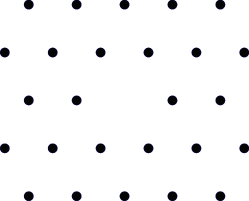
Figure 4: Schematic illustration of a point defect (vacancy) in a monatomic Bravais lattice.

Following the same procedures outlined above, we attain two expected values for the spin variables, one for each effective energy,

$$\left\langle s_{i}\right\rangle_{\text{A}}\overset{\text{def}}{=}\sum_{\left\{s_{i}\right\}}s_{i}~{}p_{\text{A}}=\tanh\left(\beta\epsilon_{\text{ND}}\right)\text{,}~{}$$ (84)

and,

$$\left\langle s_{k}\right\rangle_{\text{A}}\overset{\text{def}}{=}\sum_{\left\{s_{i}\right\}}s_{k}~{}p_{\text{A}}=\tanh\left(\beta\epsilon_{\text{D}}\right)~{}\text{.}$$ (85)

Once again, we write down the function $F_{\min}$ we wish to minimize as

$$F_{\min}=-\left\langle\mathcal{H}_{\text{A}}\right\rangle_{\text{A}}-\frac{1}{\beta}\log\mathcal{Z}_{\text{A}}+\left\langle\mathcal{H}^{\prime}\left\{s\right\}\right\rangle_{\text{A}}~{}\text{.}$$ (86)

where $\mathcal{H}^{\prime}\left\{s\right\}$ is arrived at in a similar way to Eq. (48). Substituting Eqs. (82) and (83) into Eq. (86) for $F_{\min}$ yields,

$$F_{\min} =-\left\langle-\epsilon_{\text{ND}}\sum_{i}^{N-n-1}s_{i}-\epsilon_{\text{D}}\sum_{k}^{n}s_{k}\right\rangle_{\text{A}}-\frac{1}{\beta}\log\mathcal{Z}_{\text{A}}+$$

$$+\left\langle-J\sum_{i,j}^{N-n-1,n}s_{i}s_{j}-J\sum_{k,l}^{n,n-1}s_{k}s_{l}-\sum_{i}^{N-n-1}\mu B^{\prime}s_{i}-\sum_{k}^{n}\mu B^{\prime}s_{k}\right\rangle_{\text{A}}~{}\text{.}$$ (87)

Observe that,

$$\left\langle\sum_{i}s_{i}\right\rangle_{\text{A}}=\sum_{i}\left\langle s_{i}\right\rangle_{\text{A}}=\left(N-n-1\right)\left\langle s_{i}\right\rangle_{\text{A}}=\left(N-n-1\right)\tanh\left(\beta\epsilon_{\text{ND}}\right)\text{,}$$ (88)

and,

$$\left\langle\sum_{k}s_{k}\right\rangle_{\text{A}}=\sum_{k}\left\langle s_{k}\right\rangle_{\text{A}}=n\left\langle s_{k}\right\rangle_{\text{A}}=n\tanh\left(\beta\epsilon_{\text{D}}\right)\text{.}$$ (89)

Substituting Eqs. (88) and (89) into Eq. (87), after some algebra, we obtain

$$F_{\min} =\epsilon_{\text{ND}}\left(N-n-1\right)\tanh\left(\beta\epsilon_{\text{ND}}\right)+\epsilon_{\text{D}}n\tanh\left(\beta\epsilon_{\text{D}}\right)-\frac{1}{\beta}\log\left(\mathcal{Z}_{\text{ND}}\mathcal{Z}_{\text{D}}\right)+$$

$$-J\sum_{i,j}^{N-n-1,n}\left\langle s_{i}s_{j}\right\rangle_{\text{ND}}-J\sum_{k,l}^{n,n-1}\left\langle s_{k}s_{l}\right\rangle_{\text{D}}-\mu B^{\prime}\left[\epsilon_{\text{ND}}\left(N-n-1\right)\tanh\left(\beta\epsilon_{\text{ND}}\right)+\epsilon_{\text{D}}n\tanh\left(\beta\epsilon_{\text{D}}\right)\right]~{}\text{,}$$ (90)

where $\mathcal{Z}_{\text{A}}\overset{\text{def}}{=}\mathcal{Z}_{\text{ND}}\mathcal{Z}_{\text{D}}$. Substituting $Z_{\text{ND}}\overset{N\gg 1}{\approx}\left[2\cosh\left(\beta\epsilon_{\text{ND}}\right)\right]^{\left(N-n-1\right)}$ and $Z_{\text{D}}\overset{N\gg 1}{\approx}\left[2\cosh\left(\beta\epsilon_{\text{D}}\right)\right]^{\left(n\right)}$ yields,

$$F_{\min} =\epsilon_{\text{ND}}\left(N-n-1\right)\tanh\left(\beta\epsilon_{\text{ND}}\right)+\epsilon_{\text{D}}n\tanh\left(\beta\epsilon_{\text{D}}\right)-\frac{1}{\beta}\log\left[2\cosh\left(\beta\epsilon_{\text{ND}}\right)\right]^{N-n-1}+$$

$$-\frac{1}{\beta}\log\left[2\cosh\left(\beta\epsilon_{\text{D}}\right)\right]^{n-1} -J\sum_{i,j}^{N-n-1,n}\left\langle s_{i}s_{j}\right\rangle_{\text{ND}}-J\sum_{k,l}^{n,n-1}\left\langle s_{k}s_{l}\right\rangle_{{}_{\text{D}}}-\mu B^{\prime}\left[\epsilon_{\text{ND}}\left(N-n-1\right)\tanh\left(\beta\epsilon_{\text{ND}}\right)+\epsilon_{\text{D}}n\tanh\left(\beta\epsilon_{\text{D}}\right)\right]~{}\text{.}$$ (91)

Since $\left\langle s_{i}\right\rangle_{\text{A}}$ in Eq. (84) and $\left\langle s_{k}\right\rangle_{\text{A}}$ in Eq. (85) are independent of $i$ and $k$, respectively, we have $\left\langle s_{i}\right\rangle_{\text{A}}=\left\langle s_{j}\right\rangle_{\text{A}}$ and $\left\langle s_{i}s_{j}\right\rangle_{\text{A}}=\left\langle s_{i}\right\rangle_{\text{A}}\left\langle s_{j}\right\rangle_{\text{A}}$. Therefore, we can write

$$F_{\min} =\epsilon_{\text{ND}}\left(N-n-1\right)\tanh\left(\beta\epsilon_{\text{ND}}\right)+\epsilon_{\text{D}}\left(n\right)\tanh\left(\beta\epsilon_{\text{D}}\right)-\frac{1}{\beta}\log\left[2\cosh\left(\beta\epsilon_{\text{ND}}\right)\right]^{N-n-1}-\frac{1}{\beta}\log\left[2\cosh\left(\beta\epsilon_{\text{D}}\right)\right]^{n-1}+$$

$$-J\sum_{i,j}^{N-n-1,n}\left\langle s_{i}\right\rangle_{\text{ND}}\left\langle s_{j}\right\rangle_{\text{ND}}-J\sum_{k,l}^{n,n-1}\left\langle s_{k}\right\rangle_{\text{D}}\left\langle s_{l}\right\rangle_{\text{D}}-\mu B^{\prime}\left[\epsilon_{\text{ND}}\left(N-n-1\right)\tanh\left(\beta\epsilon_{\text{ND}}\right)+\epsilon_{\text{D}}\left(n\right)\tanh\left(\beta\epsilon_{\text{D}}\right)\right]~{}\text{.}$$ (92)

Substituting Eqs. (84) and (85) into Eq. (92) yields,

$$F_{\min} =\epsilon_{\text{ND}}\left(N-n-1\right)\tanh\left(\beta\epsilon_{\text{ND}}\right)+\epsilon_{\text{D}}\left(n\right)\tanh\left(\beta\epsilon_{\text{D}}\right)-\frac{1}{\beta}\log\left[2\cosh\beta\epsilon_{\text{ND}}\right]^{N-n-1}+$$

$$-\frac{1}{\beta}\log\left[2\cosh\beta\epsilon_{\text{D}}\right]^{n-1}-\frac{1}{2}J\left(N-n-1\right)\left(n\right)\tanh^{2}\left(\beta\epsilon_{\text{ND}}\right)-\frac{1}{2}J\left(n\right)\left(n-1\right)\tanh^{2}\left(\beta\epsilon_{\text{D}}\right)+$$

$$-\mu B^{\prime}\left[\epsilon_{\text{ND}}\left(N-n-1\right)\tanh\left(\beta\epsilon_{\text{ND}}\right)+\epsilon_{\text{D}}\left(n\right)\tanh\left(\beta\epsilon_{\text{D}}\right)\right]\text{.}$$ (93)

After collecting $\epsilon_{\text{ND}}$ and $\epsilon_{\text{D}}$ like terms, we have

$$F_{\min} =\epsilon_{\text{ND}}\left(N-n-1\right)\tanh\left(\beta\epsilon_{\text{ND}}\right)-\frac{1}{\beta}\log\left[2\cosh\left(\beta\epsilon_{\text{ND}}\right)\right]^{N-n-1}+$$

$$-\frac{1}{2}J\left(N-n-1\right)\left(n\right)\tanh^{2}\left(\beta\epsilon_{\text{ND}}\right)-\mu B^{\prime}\epsilon_{\text{ND}}\left(N-n-1\right)\tanh\left(\beta\epsilon_{\text{ND}}\right)+$$

$$+\epsilon_{\text{D}}\left(n\right)\tanh\left(\beta\epsilon_{\text{D}}\right)-\frac{1}{\beta}\log\left[2\cosh\left(\beta\epsilon_{\text{D}}\right)\right]^{n-1}-\frac{1}{2}J\left(n\right)\left(n-1\right)\tanh^{2}\left(\beta\epsilon_{\text{D}}\right)-+\mu B^{\prime}\epsilon_{\text{D}}\left(n\right)\tanh\left(\beta\epsilon_{\text{D}}\right)~{}\text{,}$$ (94)

where the factor $n$ comes from the number of nearest neighbors, the factor $N$ is from the total number of atoms and the $1/2$ is due to double counting. We now choose the form that minimizes $F_{\min}$ with respect to $\epsilon_{\text{ND}}$ and $\epsilon_{\text{D}}$. When minimizing with respect to $\epsilon_{\text{ND}}$, we obtain

$$\left.\frac{\partial F_{\min}}{\partial\epsilon_{\text{ND}}}\right|_{\epsilon_{\text{ND}}=~{}\epsilon_{\text{ND}\min}} =0=\left(N-n-1\right)\tanh\left(\beta\epsilon_{\text{ND}\min}\right)+\left(N-n-1\right)\epsilon_{\text{ND}}\frac{\beta}{\cosh^{2}\left(\beta\epsilon_{\text{ND}\min}\right)}-\frac{N-n-1}{\beta}\frac{\beta\sinh\left(\beta\epsilon_{\text{ND}\min}\right)}{\cosh\left(\beta\epsilon_{\text{ND}\min}\right)}$$

$$-J\frac{1}{2}\left(N-n-1\right)\left(n\right)2\tanh\left(\beta\epsilon_{\text{ND}\min}\right)\frac{\beta}{\cosh^{2}\left(\beta\epsilon_{\text{ND}\min}\right)}-\mu B^{\prime}\left(N-n-1\right)\frac{\beta}{\cosh^{2}\left(\beta\epsilon_{\text{ND}\min}\right)}\text{,}$$ (95)

that is, after some simple algebra,

$$\epsilon_{\text{ND}\min}-\mu B^{\prime}=Jn\tanh\left(\beta\epsilon_{\text{ND}\min}\right)\text{.}$$ (96)

Similarly, when minimizing with respect to $\epsilon_{\text{D}}$, one gets

$$\epsilon_{\text{D}\min}-\mu B^{\prime}=J\left(n-1\right)\tanh\left(\beta\epsilon_{\text{D}\min}\right)\text{.}$$ (97)

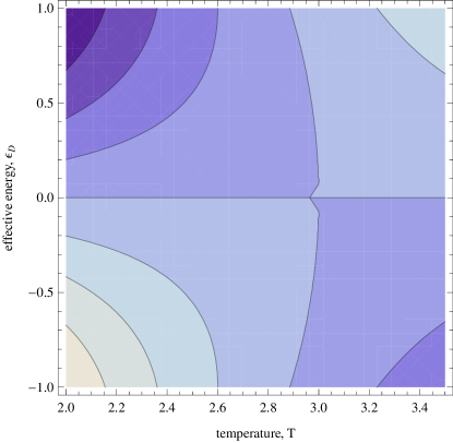
Figure 5: Contour plot exhibiting the numerical solution of the effective energy of defective atoms $\epsilon_{D}$ vs. temperature $T$. We set $k_{B}=1$ and assume $n=4$, $J=1$, $\mu=1$, $B^{\prime}=1$ and the level curves $f\left(\epsilon_{D}\text{, }T\right)=c$ with $c\in\left\{-1.3\text{, }-1.2\text{, }-1.1\text{, }-1\text{, }-0.9\right\}$.

Eqs. (96) and (97) are final results. A contour plot of $f\left(\epsilon_{\text{D}}\text{, }T\right)$ defined as,

$$f\left(\epsilon_{\text{D}}\text{, }T\right)\overset{\text{def}}{=}\epsilon_{\text{D}}-\mu B^{\prime}-J\left(n-1\right)\tanh\left(\frac{\epsilon_{\text{D}}}{k_{B}T}\right)\text{,}$$ (98)

as a function of $\epsilon_{\text{D}}$ and $T$ appears in FIG. 5. These equations can then be used as above to solve for the critical temperature, the total magnetic moment and the magnetic susceptibility for this ferromagnetic material as usual. The difference here is that we will have two of each. For example, a critical temperature that applies to most of the atoms, and one that is local to the defect. Therefore, the total magnetic moment will not simply be a result of just one temperature but a combination of each magnetic moment determined by these equations. Notice that Eq. (81) still holds in general. In the two energy case, we have for one energy the number of nearest neighbors, $n_{\text{G}}=n$ and for the second energy, $n_{\text{G}}=n-1$. As a final consideration, we point out that the outcomes of our entropic analysis in Eqs. (96) and (97) together with the numerical representation in FIG. 5 are consistent with the fact that imperfections in the lattice structure can be the cause of structural irregularities in the critical temperature $T_{c}$ jean00 ; kallin08 . However, to obtain a deeper understanding of these aspects of ferromagnetic materials from an entropic viewpoint, a more thorough analysis would be required.

Just as in the previous example, the defect could be introduced here as an observable by means of a constraint like relation,

$$\int dB\sum_{\left\{s\neq s_{0}\right\}}p\left\{s,B\right\}\equiv p\left\{s_{0}\right\}=\delta_{s_{0}\text{, }s_{0}^{\prime}}\text{ ,}$$ (99)

where $\delta_{s_{0}\text{, }s_{0}^{\prime}}$ is a Kronecker delta function. This makes much more sense here as this information may be obtained by common spectroscopic methods such as electron paramagnetic resonance, photoluminescence or cathodoluminescence. In the particular case considered here, we observed $s_{0}^{\prime}=0$.

VI Conclusive Remarks

In this article, we showed that not only can the MrE method be used for updating probability distributions with both data and expectation values, but for determining effective approximations of such probability distributions equivalent to those provided by the Bogoliubov Variational Principle and/or Mean Field Theory. Specifically, after describing the traditional Ising model of a ferromagnetic material and the mean field approximation for a multidimensional ferromagnet, we applied the MrE method to infer both magnetization and energetic features of ferromagnets characterized by simple lattice configurations. Our main results can be summarized as follows:

1. The standard mean field theory solution was recovered via MrE methods for the ferromagnetic Ising model. These findings are reported in Eq. (39) and FIG. 2. The main advantage of our analysis is the fact that we do not require the knowledge of the exact form of the effective energy $\epsilon_{\text{A}}$ and we allow for departures from the centrality of the atom.

2. Moving past traditional methods and assumptions by using MrE, we examined ferromagnets characterized by three state atoms. The outcomes of our entropic analysis are reported in Eq. (79) and FIG. 3. Based on these results, we concluded that our analysis appears to support the idea that the introduction of additional states in the atomic ferromagnetic structure is consistent with both space shifts and nonhomogeneities of the critical temperature $T_{c}$ jean00 ; kallin08 .

3. A ferromagnetic material was considered that had known defects, which is beyond the scope of the mean field methodology. These findings are presented in Eqs. (96), (97) and FIG. 5. In each case we uncovered results independent of the explicit form of the effective energy in the Hamiltonian. Relying on these results, we concluded that our research appears to be consistent with the fact that imperfections in the lattice structure can be the cause of structural irregularities in the critical temperature $T_{c}$ jean00 ; kallin08 .

4. Although it may seem trivial to introduce the observational data through an MrE constraint, as opposed to simply putting it in as would be conventionally done, it should be noted that these toy examples are mostly for pedagogical purposes in order to demonstrate how the mechanism works. The power of this methodology enters when one does not know the expectation value of the Hamiltonian, but may know how it relates to some observable, as done in giffin . For instance, a more interesting example might be a case in which the joint prior equals $p_{\text{old}}\left\{s,B\right\}=p_{\text{old}}\left\{s\right\}p_{\text{old}}\{B~{}|~{}s\}$ where $p_{\text{old}}\{B~{}|~{}s\}$ is the Bayesian likelihood that represents a model that relates some observable $B_{i}$ with $s_{i}$, like $p_{\text{old}}\{B~{}|~{}s\}\varpropto e^{-\beta\mathcal{H}_{ext}}$ with $\mathcal{H}_{ext}$ described in Eq. (45). Care must be taken when examining this scenario and such considerations will be explored in later works.

A function $f=f\left(x\right)$ can fail to be differentiable at a point $x=x_{0}$ in three scenarios: it has a vertical tangent line at $x=x_{0}$, it has a discontinuity at $x=x_{0}$, it exhibits a kink (or, corner) at $x=x_{0}$. Interestingly, we point out that Figs. $2$, $3$, and $5$ show a vertical tangent, a jump discontinuity, and a kink, respectively. Specifically, the arbitrary function $f$ is represented by the mean magnetization of the ferromagnetic material in FIG. $2$, by the effective energy of an atom in FIG. $3$, and finally, by the effective energy of a defective atom in FIG. $5$. Although numerical methods are often ineffective near points of discontinuity, our qualitative entropic analysis seems to suggest that departures from the standard Ising model (with a vertical tangent type of singularity) can lead to alternative types of non-differentiable singularities.

While the findings uncovered in this manuscript are not conclusive (about the nature of phase transitions in the presence of imperfections) by any means, this work seems to suggest that using the MrE method can be useful in inferring both thermal and electromagnetic properties of defective ferromagnetic materials in presence of available data from the substance being considered. Of course, a more detailed investigation would be required to deepen our understanding of these important phenomena in fundamental and applied science. Indeed, it is our intention to extend our study to higher order spin configurations Stanley (for example, XY spin chains, XX spin chains, Heisenberg models, or, more generally, Potts models Potts ; wu ). Finally, we point out that MrE methods employed in this article can be readily applied, in principle, to the investigation of more general dislocation, disclination, and dispiration defects in solid state physics ali07 . In particular, it would be very interesting to infer physical properties of materials exhibiting a non-uniform distribution of defects of different types. We leave these investigations to future efforts.

- (1) E. T. Jaynes, Information theory and statistical mechanics, Phys. Rev. 106, 620 (1957).
- (2) E. T. Jaynes, Information theory and statistical mechanics II, Phys. Rev. 108, 171 (1957).
- (3) C. E. Shannon, A mathematical theory of communication, Bell System Technical Journal 27, 379 (1948).
- (4) A. Caticha and A. Giffin, Updating probabilities, AIP Conf. Proc. 872, 31 (2006).
- (5) C.Y. Tseng, The Maximum Entropy Method in Statistical Physics: an Alternative Approach to the Theory of Simple Fluids, Ph. D. Thesis, SUNY at Albany, Albany-New York, USA (2004).
- (6) F. Reif, Fundamentals of Statistical and Thermal Physics, McGraw-Hill (1965).
- (7) T. D. Schultz, D. C. Mattis, and E. H. Lieb, Two-dimensional Ising model as a soluble problem of many fermions, Rev. Mod. Phys. 36, 856 (1964).
- (8) S. G. Brush, History of the Lenz-Ising model, Rev. Mod. Phys. 39, 883 (1967).
- (9) B. A. Cipra, The Ising model is NP-complete, SIAM News 33, 6 (2000).
- (10) K. Huang, Statistical Mechanics, John Wiley & Sons, Inc. (1963).
- (11) N. W. Ashcroft and N. D. Mermin, Solid State Physics, Thomson Learning, Inc. (1976).
- (12) D. V. Schroeder, An Introduction to Thermal Physics, Addison Wesley Longman (2000).
- (13) C. Cafaro and S. A. Ali, Jacobi fields on statistical manifolds of negative curvature, Physica D234, 70 (2007).
- (14) C. Cafaro, Information geometry, inference methods and chaotic energy levels statistics, Mod. Phys. Lett. B22, 1879 (2008).
- (15) C. Cafaro and S. A. Ali, Can chaotic quantum energy levels statistics be characterized using information geometry and inference methods?, Physica A387, 6876 (2008).
- (16) C. Cafaro and S. A. Ali, Geometrodynamics of information on curved statistical manifolds and its applications to chaos, EJTP 5, 139 (2008).
- (17) C. Cafaro, A. Giffin, S. A. Ali, and D.-H. Kim, Reexamination of an information geometric construction of entropic indicators of complexity, Appl. Math. Comput. 217, 2944 (2010).
- (18) C. Cafaro and S. Mancini, Quantifying the complexity of geodesic paths on curved statistical manifolds through information geometric entropies and Jacobi fields, Physica D240, 607 (2011).
- (19) D.-H. Kim, S. A. Ali, C. Cafaro, and S. Mancini, Information geometric modeling of scattering induced quantum entanglement, Phys. Lett. A375, 2868 (2011).
- (20) C. Cafaro, A. Giffin, C. Lupo, and S. Mancini, Softening the complexity of entropic motion on curved statistical manifolds, Open Systems & Information Dynamics 19, 1250001 (2012).
- (21) D. Felice, C. Cafaro, and S. Mancini, Information geometric complexity of a trivariate Gaussian statistical model, Entropy 16, 2944 (2014).
- (22) J. F. Sadoc and R. Mosseri, Geometrical Frustration, Cambridge University Press (2006).
- (23) A. Giffin and A. Caticha, Updating probabilities with data and moments, AIP Conf. Proc. 954, 74 (2007).
- (24) A. Giffin, From physics to economics: An econometric example using maximum relative entropy, Physica A388, 1610 (2009).
- (25) C.-Y. Tseng and A. Caticha, Using relative entropy to find optimal approximations: an application to simple fluids, Physica A387, 6759 (2008).
- (26) A. L. Kuzemsky, Variational principle of Bogoliubov and generalized mean fields in many-particle interacting systems, Int. J. Mod. Phys. B29, 1530010 (2015).
- (27) L. Onsager, Crystal statistics. I. A two-dimensional model with an order-disorder transition, Phys. Rev. 65, 117 (1944).
- (28) C. N. Yang, The spontaneous magnetization of a two-dimensional Ising model, Phys. Rev. 85, 808 (1952).
- (29) E. Ising, Beitrag zur theorie des ferromagnetismus, Zeitschrift fur Physik 31, 253 (1925).
- (30) P. Weiss, L’hypothese du champ moleculaire et la propriete ferromagnetique, J. Phys. Theor. Appl. 6, 661 (1907).
- (31) D. J. C. MacKay, Information Theory, Inference, and Learning Algorithms, Cambridge University Press (2003).
- (32) H. E. Stanley, Introduction to phase transitions and critical phenomena, Oxford University Press (1971).
- (33) A. Caticha, Entropic Inference and the Foundations of Physics, USP Press, Sao Paulo, Brazil (2012).
- (34) F. Jean, G. Collin, M. Andrieux, N. Blanchard, J.-F. Marucco, Oxygen nonstoichiometry, point defects and critical temperature in superconducting oxide Bi2Sr2CaCu2O8+Δ, Physica C339, 269 (2000).
- (35) D. Davidovich, A. J. Berlinsky, and C. Kallin, Superfluid density near the critical temperature in the presence of random planar defects, Phys. Rev. B78, 214508 (2008).
- (36) J. Ashkin and E. Teller, Statistics of two-dimensional lattices with four components, Phys. Rev. 64, 178 (1943).
- (37) H. E. Stanley, Dependence of critical properties upon dimensionality of spins, Phys. Rev. Lett. 20, 589 (1968).
- (38) R. B. Potts, Some Generalized Order-Disorder Transformations, Mathematical Proceedings 48, 106 (1952).
- (39) F. Y. Wu, The Potts model, Rev. Mod. Phys. 54, 235 (1982).
- (40) S. A. Ali, C. Cafaro, S. Capozziello, and Ch. Corda, A bound quantum particle in a Riemann-Cartan space with topological defects and planar potential, Phys. Lett. A366, 315 (2007).