The chirally rotated Schrödinger functional: theoretical expectations and perturbative tests

Abstract

The chirally rotated Schrödinger functional ($\chi$SF) with massless Wilson-type fermions provides an alternative lattice regularization of the Schrödinger functional (SF), with different lattice symmetries and a common continuum limit expected from universality. The explicit breaking of flavour and parity symmetries needs to be repaired by tuning the bare fermion mass and the coefficient of a dimension 3 boundary counterterm. Once this is achieved one expects the mechanism of automatic O($a$) improvement to be operational in the $\chi$SF, in contrast to the standard formulation of the SF. This is expected to significantly improve the attainable precision for step-scaling functions of some composite operators. Furthermore, the $\chi$SF offers new strategies to determine finite renormalization constants which are traditionally obtained from chiral Ward identities. In this paper we consider a complete set of fermion bilinear operators, define corresponding correlation functions and explain the relation to their standard SF counterparts. We discuss renormalization and O($a$) improvement and then use this set-up to formulate the theoretical expectations which follow from universality. Expanding the correlation functions to one-loop order of perturbation theory we then perform a number of non-trivial checks. In the process we obtain the action counterterm coefficients to one-loop order and reproduce some known perturbative results for renormalization constants of fermion bilinears. By confirming the theoretical expectations, this perturbative study lends further support to the soundness of the $\chi$SF framework and prepares the ground for non-perturbative applications.

1 Introduction

The chirally rotated Schrödinger functional ($\chi$SF) Sint:2005qz ; Sint:2010eh provides a new tool to address renormalization and O($a$) improvement problems in lattice QCD and similar lattice gauge theories with Wilson type fermions. With an even number of massless fermion flavours it is formally related to the standard Schrödinger functional (SF) Luscher:1992an ; Sint:1993un ; Sint:1995rb by a non-singlet chiral field rotation. Such chirally rotated SF boundary conditions have first appeared with staggered fermions Miyazaki:1994nu where the chiral rotation can be absorbed in the reconstruction of four-spinors from the one-component staggered fermion field Heller:1997pn ; PerezRubio:2008yd . Similarly, with Ginsparg-Wilson or domain-wall fermions such boundary conditions Taniguchi:2004gf ; Taniguchi:2006qw can be re-interpreted as standard SF boundary conditions, based on exact Ginsparg-Wilson-type lattice symmetries Sint:2007zz . With Wilson fermions the chiral field rotation does not correspond to a lattice symmetry, and the $\chi$SF can thus be seen as an alternative lattice regularization of the SF. The $\chi$SF has practical advantages when applied to non-perturbative renormalization problems. In particular, the expected property of automatic O($a$) improvement Frezzotti:2003ni ; Sint:2010eh will potentially be very helpful in reducing systematic errors in continuum extrapolations of step-scaling functions. The theoretical framework for the $\chi$SF has been defined in ref. Sint:2010eh where also some perturbative tests have been performed at tree-level. Here we would like to define the framework for systematic tests and applications of the $\chi$SF. In particular we define boundary-to-boundary correlation functions, as well as boundary-to-bulk correlation functions for a complete set of non-singlet fermion bilinear operators. We then establish a dictionary translating them to their SF counterparts. This is reminiscent of twisted mass QCD Frezzotti:2000nk , except that we will here exclusively focus on the massless theory. From universality one then expects that the same dictionary holds in terms of renormalized correlation functions up to cutoff effects. We formulate various consequences of this expectation such as flavour and parity symmetry restoration, the possibility to determine finite renormalization constants (otherwise obtainable by chiral Ward identities), and scale dependent renormalization constants in SF schemes, together with their step-scaling functions. We then use one-loop perturbation theory to perform non-trivial tests of these expectations. Some elements of the set-up together with tests in quenched QCD have already appeared in ref. Sint:2010xy , and preliminary one-loop results have been given in refs. Sint:2011gv ; Sint:2012ae ; Sint:2014wwa . For related non-perturbative applications of the $\chi$SF to quenched lattice QCD cf. refs. Lopez:2012as ; Lopez:2012mc . Preliminary results for two-flavour lattice QCD can be found in ref. Brida:2014zwa .

The paper is organized as follows: in Section 2 we use a continuum language to discuss the connection between the SF and the $\chi$SF and the respective correlation functions of interest. The transcription to the lattice regularization is described in Section 3, followed by a discussion of renormalization and Symanzik O($a$) improvement, for both the standard SF and the $\chi$SF. In Section 4 we summarize the theoretical expectations for the $\chi$SF. The remainder of this paper discusses the perturbative expansion and one-loop results for the action parameters (Section 5) and various ways to test and apply the theoretical expectations in perturbation theory (Sects. 6 and 7). Section 8 contains a discussion of a gluonic observable, the SF coupling, to one-loop order. Conclusions are drawn in Section 9, and 3 appendices collect some definitions regarding fermion bilinear fields (Appendix A), a few details on the calculation of the fermionic contribution to the SF coupling at one-loop order (Appendix B) and a comparison at weak coupling between perturbation theory and Monte-Carlo simulations (Appendix C).

2 Correlation functions and universality relations

In this section we recall the formal continuum relations between SF and $\chi$SF correlation functions, which are obtained by a change of variables in the functional integral of the formal continuum theory. We then establish a dictionary between specific SF and $\chi$SF correlation functions of non-singlet fermion bilinear operators. On the lattice with Wilson type fermions the chiral symmetry relating the SF and the $\chi$SF is broken explicitly. Therefore the relation between both formulations is expected to assume the simple form of the continuum dictionary only after appropriate renormalization and up to cutoff effects.

2.1 Chiral rotations and correlation functions

The continuum action for ${N_{\rm f}}$ massless fermions in an external gauge field $A_{\mu}(x)$,

$$S_{f}=\int{\rm d}^{4}x\,\,\bar{\psi}(x)\gamma_{\mu}D_{\mu}\psi(x),\qquad D_{\mu}=\partial_{\mu}+A_{\mu},$$ (1)

has exact flavour and chiral symmetries. The latter are broken if one imposes the standard SF boundary conditions on the fermionic fields,

$$P_{+}\psi(x)|_{x_{0}=0} =0, P_{-}\psi(x)|_{x_{0}=T} =0,$$

$$\bar{\psi}(x)P_{-}|_{x_{0}=0} =0, \bar{\psi}(x)P_{+}|_{x_{0}=T} =0,$$ (2)

with the projectors $P_{\pm}={\tfrac{1}{2}}(1\pm\gamma_{0})$. Indeed, assuming ${N_{\rm f}}=2$ flavours, a chiral non-singlet transformation,

$$\psi=R(\pi/2)\psi^{\prime},\qquad\bar{\psi}=\bar{\psi}^{\prime}R(\pi/2),$$ (3)

with $R(\alpha)=\exp(i\alpha\gamma_{5}\tau^{3}/2)$, transforms Eqs. (2) to

$$\tilde{Q}_{+}\psi^{\prime}(x)|_{x_{0}=0} =0, \tilde{Q}_{-}\psi^{\prime}(x)|_{x_{0}=T} =0,$$

$$\bar{\psi}^{\prime}(x)\tilde{Q}_{+}|_{x_{0}=0} =0, \bar{\psi}^{\prime}(x)\tilde{Q}_{-}|_{x_{0}=T} =0\,,$$ (4)

where

$$\tilde{Q}_{\pm}={\tfrac{1}{2}}(1\pm i\gamma_{0}\gamma_{5}\tau^{3}),$$ (5)

and the Pauli matrix $\tau^{3}$ acts on the flavour indices. If the field transformation is performed as a change of variables in the functional integral one obtains relations between standard SF and $\chi$SF correlation functions,

$$\left\langle O[\psi,\bar{\psi}]\right\rangle_{(\tilde{Q}_{+})} = \left\langle O[R(-\pi/2)\psi,\bar{\psi}R(-\pi/2)]\right\rangle_{(P_{+})},$$ (6)

$$\left\langle O[\psi,\bar{\psi}]\right\rangle_{(P_{+})} = \left\langle O[R(\pi/2)\psi,\bar{\psi}R(\pi/2)]\right\rangle_{(\tilde{Q}_{+})}.$$ (7)

Here, the subscript to the correlation function indicates the projector defining the Dirichlet component of the fermion field at $x_{0}=0$. This notation unambiguously specifies the boundary conditions for the integration variables in the functional integral, which we will always denote by $\psi$ and $\bar{\psi}$, thereby removing the prime from the fields in the $\chi$SF. Note also that the composite fields $O[\psi,\bar{\psi}]$ inside correlation functions may include the boundary fermion fields,

$$\zeta({\bf x}) =\psi(0_{+},{\bf x}), \bar{\zeta}({\bf x}) =\bar{\psi}(0_{+},{\bf x}),$$ (8)

$$\zeta\kern 1.0pt^{\prime}({\bf x}) =\psi(T_{-},{\bf x}), \bar{\zeta}\kern 1.0pt^{\prime}({\bf x}) =\bar{\psi}(T_{-},{\bf x}).$$ (9)

The time arguments $0_{+}$ or $T_{-}$ indicate that the fields are located infinitesimally away from the boundaries at $x_{0}=0,T$. For later convenience we have omitted the projectors $P_{\pm}$ or $\tilde{Q}_{\pm}$, in contrast to conventions used in the literature Luscher:1996sc ; Sint:2010eh . Instead we include these projectors explicitly when defining the bilinear boundary source fields for SF and $\chi$SF correlation functions (cf. Subsections 2.3,2.4).

2.2 Flavour structure and symmetries

While the standard SF can be formulated for any number of flavours, this is not straightforward for the $\chi$SF Sint:2010eh . We will restrict attention to gauge theories with an even number of fermion flavours. So far we have assumed ${N_{\rm f}}=2$, i.e. a doublet structure,

$$\psi=\begin{pmatrix}\psi_{u}\\ \psi_{d}\end{pmatrix},$$ (10)

with up and down type flavours. For the correlation functions defined below it will be convenient to introduce more than a single up or down type flavour, such that flavour non-singlet fermion bilinear fields can be formed with only up- or only down-type fermions. We are thus led to consider the case ${N_{\rm f}}=4$ which we obtain by replicating the doublet structure,

$$\psi=\begin{pmatrix}\psi_{u}\\ \psi_{d}\\ \psi_{u^{\prime}}\\ \psi_{d^{\prime}}\end{pmatrix},$$ (11)

i.e. there are two up and two down type flavours. Obviously this implies that the flavour matrix $\tau^{3}$ in Eqs. (3),(5) should be replaced by

$$\tau^{3}\rightarrow 1\kern-2.5pt{\rm l}_{2}\otimes\tau^{3}={\rm diag}(1,-1,1,-1).$$ (12)

It is often convenient to reduce the flavour structure of the projectors,

$$\left.\tilde{Q}\right|_{{N_{\rm f}}=2}={\rm diag}(Q_{+},Q_{-}),\qquad\left.\tilde{Q}\right|_{{N_{\rm f}}=4}={\rm diag}(Q_{+},Q_{-},Q_{+},Q_{-}),$$ (13)

with

$$Q_{\pm}={\tfrac{1}{2}}(1\pm i\gamma_{0}\gamma_{5}).$$ (14)

Although the $\chi$SF boundary conditions differ for up and down type flavours, this does not mean that the SU(${N_{\rm f}}$) flavour symmetry is broken. In fact, as discussed in ref. Sint:2010eh , the distinction between flavour and chiral symmetries in the absence of mass terms is conventional. We here follow the convention used in ref. Sint:2010eh and define the flavour symmetry such that the corresponding field transformations take their usual form in the standard SF basis. In this basis, a flavour transformation for ${N_{\rm f}}=2$ flavours with parameters $\omega^{a}$ ($a=1,2,3$), looks as usual,

$$\psi\rightarrow\exp\left(i\sum_{a=1}^{3}\omega^{a}\tau^{a}\right)\psi,\qquad\bar{\psi}\rightarrow\bar{\psi}\exp\left(-i\sum_{a=1}^{3}\omega^{a}\tau^{a}\right).$$ (15)

As the SF and $\chi$SF fields are related by the chiral rotation (3) the same flavour symmetry transformation on the $\chi$SF fields takes the form

$$\psi^{\prime} \rightarrow R(-\pi/2)\exp\left(i\sum_{a=1}^{3}\omega^{a}\tau^{a}\right)R(\pi/2)\psi^{\prime},$$ (16)

$$\bar{\psi}^{\prime} \rightarrow \bar{\psi}^{\prime}\,R(\pi/2)\exp\left(-i\sum_{a=1}^{3}\omega^{a}\tau^{a}\right)R(-\pi/2).$$ (17)

In particular, in the continuum the $\chi$SF shares all the symmetries with the standard SF, i.e. the full flavour symmetry, charge conjugation, spatial rotations and parity. Of particular interest is the parity symmetry, which in the SF basis is realized by

$$P:\begin{cases}\psi(x)\rightarrow\gamma_{0}\psi(\tilde{x}),\\ \bar{\psi}(x)\rightarrow\bar{\psi}(\tilde{x})\gamma_{0},\end{cases}\qquad\tilde{x}=(x_{0},-{\bf x}),$$ (18)

whereas its covariantly rotated $\chi$SF version reads,

$$P_{5}:\begin{cases}\psi^{\prime}(x)\rightarrow i\gamma_{0}\gamma_{5}\tau^{3}\psi^{\prime}(\tilde{x}),\\ \bar{\psi}^{\prime}(x)\rightarrow-\bar{\psi}^{\prime}(\tilde{x})i\gamma_{0}\gamma_{5}\tau^{3},\end{cases}\qquad\tilde{x}=(x_{0},-{\bf x}).$$ (19)

The $P_{5}$-symmetry plays an important rôle in the following, as it may be used to classify lattice correlation functions and their approach to the continuum limit. More precisely, in the lattice regularized $\chi$SF the $P_{5}$-even correlation functions are automatically O($a$) improved in the bulk, whereas their $P_{5}$-odd counterparts are pure lattice artefacts. Hence, $P_{5}$ may be taken as a substitute for the $\gamma_{5}\tau^{1}$ symmetry used in ref. Sint:2010eh ,

$$\psi^{\prime}\rightarrow\gamma_{5}\tau^{1}\psi^{\prime},\qquad\bar{\psi}^{\prime}\rightarrow-\bar{\psi}^{\prime}\gamma_{5}\tau^{1},$$ (20)

which corresponds to a discrete flavour symmetry. The advantage of $P_{5}$ is that it is flavour diagonal and therefore more suitable for $\chi$SF correlation functions with specific flavour assignments.

2.3 SF correlation functions

The SF correlation functions required for this work have previously appeared in the literature, e.g. in refs. Luscher:1996sc ; Sint:1997jx . When written in terms of fixed flavours, $f_{1},f_{2}\in\{u,d,u^{\prime},d^{\prime}\}$, with $f_{1}\neq f_{2}$, they take the form

$$f_{\rm X}(x_{0})=-{1\over 2}\langle X^{f_{1}f_{2}}(x)\mathcal{O}_{5}^{f_{2}f_{1}}\rangle_{(P_{+})},\qquad k_{\rm Y}(x_{0})=-{1\over 6}\sum_{k=1}^{3}\langle Y_{k}^{f_{1}f_{2}}(x)\mathcal{O}_{k}^{f_{2}f_{1}}\rangle_{(P_{+})}.$$ (21)

In the literature, the composite fields $X$ and $Y_{k}$ stand for the fermion bilinears $X=A_{0},P$ and $Y_{k}=V_{k},T_{k0}$. Here we also include $X=V_{0},S$ and $Y_{k}=A_{k},\widetilde{T}_{k0}$. While these additional correlation functions are odd under parity (18) and thus vanish exactly, we will need them for the dictionary with their $\chi$SF counterparts defined below. Finally, the fermion bilinear source fields at the lower time boundary are defined by

$${\cal O}_{5}^{f_{1}f_{2}} =\int{\rm d}^{3}{\bf y}{\rm d}^{3}{\bf z}\,\,\bar{\zeta}_{f_{1}}({\bf y})P_{+}\gamma_{5}\zeta_{f_{2}}({{\bf z}}),$$ (22)

$${\cal O}_{k}^{f_{1}f_{2}} =\int{\rm d}^{3}{\bf y}{\rm d}^{3}{\bf z}\,\,\bar{\zeta}_{f_{1}}({\bf y})P_{+}\gamma_{k}\zeta_{f_{2}}({{\bf z}}).$$ (23)

Note that the projector $P_{+}$ must be written explicitly as we did not include it in the definition of the fermionic boundary fields $\zeta$ and $\bar{\zeta}$, Eq. (8). Integrating over the fermion fields in the functional integral one obtains, for example,

$$f_{\rm A}(x_{0})=\frac{1}{2}\int{\rm d}^{3}{\bf y}{\rm d}^{3}{\bf z}\left\langle{\rm tr}\left\{S(x;0,{\bf y})P_{+}\gamma_{5}P_{-}S(0,{\bf z};x)\gamma_{0}\gamma_{5}\right\}\right\rangle_{G},$$ (24)

where $\langle\cdots\rangle_{G}$ denotes the gauge field average, $S(x,y)$ the propagator for a single fermion flavour, and the trace is to be taken over colour and Dirac indices. The SF boundary conditions in terms of the fermion propagator,

$$P_{+}S(x,y)|_{x_{0}=0}=0=S(x,y)P_{-}|_{y_{0}=0},$$ (25)

now imply that the correlation function vanishes if the projector in Eq. (22) is reverted, $P_{+}\rightarrow P_{-}$. In the lattice regularized theory this only holds after taking the continuum limit and may thus be used as a check. Finally, we also need the boundary-to-boundary correlators,

$$f_{1}=-\frac{1}{2}\left\langle{\cal O}_{5}^{f_{1}f_{2}}{\cal O}_{5}^{{}^{\prime}f_{2}f_{1}}\right\rangle_{(P_{+})},\qquad k_{1}=-\frac{1}{6}\sum_{k=1}^{3}\left\langle{\cal O}_{k}^{f_{1}f_{2}}{\cal O}_{k}^{{}^{\prime}f_{2}f_{1}}\right\rangle_{(P_{+})}\,,$$ (26)

where the fermion bilinear source fields at the upper time boundary are defined by

$${\cal O}_{5}^{{}^{\prime}f_{1}f_{2}} = \int{\rm d}^{3}{\bf y}{\rm d}^{3}{\bf z}\,\,\bar{\zeta}\kern 1.0pt^{\prime}_{f_{1}}({\bf y})P_{-}\gamma_{5}\zeta\kern 1.0pt^{\prime}_{f_{2}}({{\bf z}}),$$ (27)

$${\cal O}_{k}^{{}^{\prime}f_{1}f_{2}} = \int{\rm d}^{3}{\bf y}{\rm d}^{3}{\bf z}\,\,\bar{\zeta}\kern 1.0pt^{\prime}_{f_{1}}({\bf y})P_{-}\gamma_{k}\zeta\kern 1.0pt^{\prime}_{f_{2}}({{\bf z}}).$$ (28)

2.4 $\chi$SF correlation functions

To obtain correlation functions in the $\chi$SF we apply the identities (6),(7) to the standard SF correlation functions. First we define the bilinear source fields ${\cal Q}_{5}^{f_{1}f_{2}}$ and ${\cal Q}_{k}^{f_{1}f_{2}}$ such that they rotate into the standard SF sources (22),(23), i.e.

$$\langle O[R(\pi/2)\psi,\bar{\psi}R(\pi/2)]{\cal Q}_{5,k}^{f_{1}f_{2}}\rangle_{(\tilde{Q}_{+})}=\langle O[\psi,\bar{\psi}]{\cal O}_{5,k}^{f_{1}f_{2}}\rangle_{(P_{+})},$$ (29)

and the same for the primed source fields at the upper time boundary. In this way one obtains, for example,

$${\cal Q}_{5}^{uu^{\prime}} = \int{\rm d}^{3}{\bf y}{\rm d}^{3}{\bf z}\,\,\bar{\zeta}_{u}({\bf y})\gamma_{0}\gamma_{5}Q_{-}\zeta_{u^{\prime}}({{\bf z}}),$$ (30)

$${\cal Q}_{5}^{du} = \int{\rm d}^{3}{\bf y}{\rm d}^{3}{\bf z}\,\,\bar{\zeta}_{d}({\bf y})\gamma_{5}Q_{-}\zeta_{u}({{\bf z}}),$$ (31)

and the complete set of source fields can be found in Appendix A.

We now define the correlation functions for fermion bilinears $X=V_{0},A_{0},S,P$, by

$$g_{\rm X}^{f_{1}f_{2}}(x_{0})=-\frac{1}{2}\left\langle X^{f_{1}f_{2}}(x){\cal Q}_{5}^{f_{2}f_{1}}\right\rangle_{(\tilde{Q}_{+})},$$ (32)

where we label the correlation functions by the flavour indices of the fermion bilinear operator in the bulk. It is then straightforward to work out the relations (6),(7) for these particular correlation functions:

$$f_{\rm A}\, = \,g_{\rm A}^{uu^{\prime}} = \,g_{\rm A}^{dd^{\prime}} = \,-ig_{\rm V}^{ud} =\,ig_{\rm V}^{du},$$ (33)

$$f_{\rm P}\, = \,ig_{\rm S}^{uu^{\prime}} = \,-ig_{\rm S}^{dd^{\prime}} = \,g_{\rm P}^{ud} =\,\phantom{i}g_{\rm P}^{du},$$ (34)

$$f_{\rm V}\, = \,g_{\rm V}^{uu^{\prime}} = \,g_{\rm V}^{dd^{\prime}} = \,-ig_{\rm A}^{ud} =\,ig_{\rm A}^{du},$$ (35)

$$f_{\rm S}\, = \,ig_{\rm P}^{uu^{\prime}} = \,-ig_{\rm P}^{dd^{\prime}} = \,g_{\rm S}^{ud} =\,\phantom{i}g_{\rm S}^{du}.$$ (36)

Hence, by using the chirally covariant definition of the boundary source fields, Eqs. (30) and (31), the properties of the correlation functions $g_{\rm X}$ under chiral rotations are the same as for the inserted fermion bilinear operators.

Proceeding similarly for the source fields with an open spatial vector index, Eq. (23), the correlation functions of the bilinear fields $Y_{k}=A_{k},V_{k},T_{k0},\widetilde{T}_{k0}$ are defined by

$$l_{\rm Y}^{f_{1}f_{2}}(x_{0})=-\frac{1}{6}\sum_{k=1}^{3}\left\langle Y_{k}^{f_{1}f_{2}}(x){\cal Q}_{k}^{f_{2}f_{1}}\right\rangle_{(\tilde{Q}_{+})},$$ (37)

and their relations to the standard SF correlation functions are found to be,

$$k_{\rm V} = \,l_{\rm V}^{uu^{\prime}} = \,l_{\rm V}^{dd^{\prime}} = \,-il_{\rm A}^{ud} =\,il_{\rm A}^{du},$$ (38)

$$k_{\rm A} = \,l_{\rm A}^{uu^{\prime}} = \,l_{\rm A}^{dd^{\prime}} = \,-il_{\rm V}^{ud} =\,il_{\rm V}^{du},$$ (39)

$$k_{\rm T} = \,il_{\rm\widetilde{T}}^{uu^{\prime}} = \,-il_{\rm\widetilde{T}}^{dd^{\prime}} = \,l_{\rm T}^{ud} =\,\phantom{i}l_{\rm T}^{du},$$ (40)

$$k_{\rm\widetilde{T}} = \,il_{\rm T}^{uu^{\prime}} = \,-il_{\rm T}^{dd^{\prime}} = \,l_{\rm\widetilde{T}}^{ud} =\,\phantom{i}l_{\rm\widetilde{T}}^{du}\,.$$ (41)

Finally, boundary-to-boundary correlators are defined by

$$g_{1}^{f_{1}f_{2}} = -\frac{1}{2}\left\langle{\cal Q}_{5}^{f_{1}f_{2}}{\cal Q}_{5}^{{}^{\prime}f_{2}f_{1}}\right\rangle_{(\tilde{Q}_{+})},$$ (42)

$$l_{1}^{f_{1}f_{2}} = -\frac{1}{6}\sum_{k=1}^{3}\left\langle{\cal Q}_{k}^{f_{1}f_{2}}{\cal Q}_{k}^{{}^{\prime}f_{2}f_{1}}\right\rangle_{(\tilde{Q}_{+})}.$$ (43)

Again, the primed sources at the upper time boundary are chirally mapped to their standard SF counterparts, leading to rather simple entries for our dictionary,

$$f_{1} = \,g_{1}^{uu^{\prime}} = \,g_{1}^{dd^{\prime}} = \,g_{1}^{ud} =\,g_{1}^{du}\,,$$ (44)

$$k_{1} = \,l_{1}^{uu^{\prime}} = \,l_{1}^{dd^{\prime}} = \,l_{1}^{ud} =\,l_{1}^{du}.$$ (45)

Note that, in the continuum, there are only 6 independent non-zero correlation functions, namely $f_{\rm A},f_{\rm P},f_{1}$ and $k_{\rm V},k_{\rm T},k_{1}$ and the corresponding $\chi$SF correlation functions can be looked up in the dictionary. As the standard SF correlation functions are real-valued, their $\chi$SF counterparts must be either real or purely imaginary. While this dictionary is trivial in the formal continuum theory, it does however lead to non-trivial consequences once the lattice regularization with Wilson-type fermions is in place, due to the additional symmetry breaking by the Wilson term.

3 Lattice set-up, renormalization and O($a$) improvement

The lattice formulation of the standard Schrödinger functional on a lattice of spacing $a$ and size $(T/a)\times(L/a)^{3}$ is taken over from ref. Luscher:1996sc . The chirally rotated Schrödinger functional will be used in the form described in ref. Sint:2010eh . We refer to these references for unexplained notation.

3.1 Lattice actions

The lattice action,

$$S[U,\psi,\bar{\psi}]=S_{g}[U]+S_{f}[U,\psi,\bar{\psi}],$$ (46)

consists of a pure gauge and a fermionic part. For the former we choose Wilson’s plaquette action Luscher:1992an ,

$$S_{g}[U]=\dfrac{1}{g_{0}^{2}}\sum_{p}w(p){\rm tr}\{1-U(p)\},$$ (47)

where the sum is over all oriented plaquettes $p$, and $U(p)$ denotes the parallel transporter around $p$, constructed from the link variables $U_{\mu}(x)$. We choose $L$-periodic boundary conditions in all the spatial directions,

$$U_{\mu}(x+L\hat{\bf k})=U_{\mu}(x),\qquad k=1,2,3,$$ (48)

where $\hat{\bf k}$ denotes a unit vector in direction $k$. In the Euclidean time direction we choose homogeneous boundary conditions for the spatial gauge potential at $x_{0}=0,T$, i.e. the spatial link variables at the boundaries are set to unit matrices,

$$U_{k}(0,{\bf x})=1\kern-2.5pt{\rm l}=U_{k}(T,{\bf x}),\quad k=1,2,3\,.$$ (49)

With these boundary conditions, the weight factors $w(p)$ take the values

$$w(p)=\begin{cases}c_{\rm t}(g_{0})&\text{if $p$ is a time like plaquette attached to a boundary plane,}\\ 1&\text{otherwise.}\end{cases}$$ (50)

Here $c_{\rm t}$ is an O($a$) boundary counterterm coefficient. Near the continuum limit it is seen to multiply the dimension 4 operator ${\rm tr}\{F_{0k}F_{0k}\}$, where $F_{\mu\nu}$ denotes the gluonic field strength tensor. Disregarding fermion fields, this operator is the only non-vanishing boundary counterterm at order $a$ given our choice of boundary conditions. Hence, all O($a$) effects in the pure gauge theory can be cancelled by choosing $c_{\rm t}(g_{0})$ appropriately.

The fermionic fields $\psi$ and $\bar{\psi}$ are taken to be $L$-periodic in space,

$$\psi(x+L\hat{\bf k})=\psi(x),\qquad\bar{\psi}(x+L\hat{\bf k})=\bar{\psi}(x),\qquad k=1,2,3.$$ (51)

Apart from the SU($N$) gauge field, the fermions are coupled to a constant U(1) background field $\lambda_{\mu}=\exp(ia\theta_{\mu}/L)$, so that the covariant forward and backward derivatives are given by

$$\nabla_{\mu}\psi(x) = \frac{1}{a}\big{[}\lambda_{\mu}U_{\mu}(x)\psi(x+a\hat{\mu})-\psi(x)\big{]},$$ (52)

$$\nabla_{\mu}^{\ast}\psi(x) = \frac{1}{a}\big{[}\psi(x)-\lambda_{\mu}^{-1}U_{\mu}(x-a\hat{\mu})^{\dagger}\psi(x-a\hat{\mu})\big{]}.$$ (53)

We will always assume $\theta_{0}=0$ and $\theta_{k}=\theta$ ($k=1,2,3$), leaving $\theta$ as a single parameter. On a lattice with infinite Euclidean time extent the Wilson-Dirac operator can be written as a finite difference operator in time,

$$aD_{W}\psi(x)=-U_{0}(x)P_{-}\psi(x+a\hat{\bf 0})+K\psi(x)-U_{0}(x-a\hat{\bf 0})^{\dagger}P_{+}\psi(x-a\hat{\bf 0}),$$ (54)

with the time diagonal operator $K$,

$$K\psi(x) = \left(1+\frac{1}{2}\sum_{k=1}^{3}\left\{a(\nabla_{k}+\nabla^{\ast}_{k})\gamma_{k}-a^{2}\nabla^{\ast}_{k}\nabla_{k}\right\}\right)\psi(x)$$ (55)

$$\mbox{}+c_{\rm sw}\frac{i}{4}a^{2}\sum_{\mu,\nu=0}^{3}\sigma_{\mu\nu}\hat{F}_{\mu\nu}(x)\psi(x).$$

Here, the last term is the Sheikholeslami-Wohlert (SW) term Sheikholeslami:1985ij in the notation of ref. Luscher:1996sc . Using a continuum-like normalisation, the fermionic action for either the standard SF or the $\chi$SF takes the form,

$$S_{f}[U,\psi,\bar{\psi}]=a^{4}\sum_{x}\bar{\psi}(x)\left({\cal D}_{W}+\delta{\cal D}_{W}+m_{0}\right)\psi(x)\,,$$ (56)

where ${\cal D}_{W}$ is the reduction of the Wilson-Dirac operator to the finite time interval between $x_{0}=0$ and $x_{0}=T$, which incorporates the respective boundary conditions, and $\delta{\cal D}_{W}$ arises due to the fermionic boundary counterterms.

In the case of the $\chi$SF, three different versions have been proposed in ref. Sint:2010eh and we here choose

$$a{\cal D}_{W}\psi(x)=\begin{cases}-U_{0}(x)P_{-}\psi(x+a\hat{\bf 0})+(K|_{c_{\rm sw}=0}+i\gamma_{5}\tau^{3}P_{-})\psi(x)&\text{if $x_{0}=0$,}\\ aD_{W}\psi(x)&\text{if $0<x_{0}<T$,}\\ (K|_{c_{\rm sw}=0}+i\gamma_{5}\tau^{3}P_{+})\psi(x)-U_{0}(x-a\hat{\bf 0})^{\dagger}P_{+}\psi(x-a\hat{\bf 0})&\text{for $x_{0}=T$.}\\ \end{cases}$$ (57)

Note that the dynamical field variables here include the fermion fields at Euclidean times $x_{0}=0$ and $x_{0}=T$, i.e. the sum over $x_{0}$ in Eq. (56) runs from $0$ to $T$. If the Sheikholeslami-Wohlert term is included we set it to zero at the boundaries, even though the orbifold construction yields a different prescription Sint:2010eh . The difference in the action is of O($a^{2}$) and thus irrelevant. The boundary counterterms for the $\chi$SF are included by setting

$$\delta{\cal D}_{W}\psi(x) = \left(\delta_{x_{0},0}+\delta_{x_{0},T}\right)\Bigl{[}\left(z_{f}-1\right)+\left(d_{s}-1\right)a{\bf D}_{s}\Bigr{]}\psi(x),$$ (58)

$${\bf D}_{s} = \frac{1}{2}\sum_{k=1}^{3}\left\{(\nabla_{k}+\nabla^{\ast}_{k})\gamma_{k}-a\nabla^{\ast}_{k}\nabla_{k}\right\},$$ (59)

and the values for the two coefficients, $z_{f}$ and $d_{s}$ will be specified in Sect. 4. Note that this definition of ${\bf D}_{s}$ differs from Sint:2010eh in that it also includes a second order derivative term.

The Wilson-Dirac operator for the standard SF in the same notation reads

$$a{\cal D}_{W}\psi(x)=\begin{cases}-U_{0}(x)P_{-}\psi(x+a\hat{\bf 0})+K\psi(x)&\text{if $x_{0}=a$\,,}\\ aD_{W}\psi(x)&\text{if $a<x_{0}<T-a$\,,}\\ K\psi(x)-U_{0}(x-a\hat{\bf 0})^{\dagger}P_{+}\psi(x-a\hat{\bf 0})&\text{for $x_{0}=T-a$\,.}\\ \end{cases}$$ (60)

In contrast to our chosen set-up for the $\chi$SF the dynamical fermionic field variables in the standard SF are restricted to Euclidean times $0<x_{0}<T$, i.e. the sum over $x_{0}$ in Eq. (56) runs only from $a$ to $T-a$. Finally, in the standard SF, the counterterm contribution is given by

$$a\delta{\cal D}_{W}\psi(x)=(\tilde{c}_{\rm t}-1)\left(\delta_{x_{0},a}+\delta_{x_{0},T-a}\right)\psi(x).$$ (61)

3.2 Lattice correlation functions

The correlation functions introduced in Sect. 2 can now easily be transcribed to the lattice. One essentially needs to specify the boundary quark fields $\zeta$ and $\bar{\zeta}$ at time $x_{0}=0$ and $\zeta\kern 1.0pt^{\prime}$ and $\bar{\zeta}\kern 1.0pt^{\prime}$ at time $x_{0}=T$. As before we leave out the projectors here and the notation is therefore the same for both the SF and the $\chi$SF, i.e. in expectation values one performs the replacement,

$$\zeta_{f}({\bf x}) =U_{0}(0,{\bf x})\psi_{f}(a,{\bf x}), \zeta\kern 1.0pt^{\prime}_{f}({\bf x}) =U_{0}(T-a,{\bf x})^{\dagger}\psi_{f}(T-a,{\bf x}),$$ (62)

$$\bar{\zeta}_{f}({\bf x}) =\bar{\psi}_{f}(a,{\bf x})U_{0}(0,{\bf x})^{\dagger}, \bar{\zeta}\kern 1.0pt^{\prime}_{f}({\bf x}) =\bar{\psi}_{f}(T-a,{\bf x})U_{0}(T-a,{\bf x}).$$ (63)

Note that this correspondence is incomplete if the Wick contractions include two-point functions with source and sink at the same boundary Luscher:1996sc ; Sint:2010eh . Here we avoid this problem by our choice of flavour assignments in the correlation functions of Sect. 2. Moreover, in the case of the $\chi$SF we have left out the O($a$) counterterm proportional to $\bar{d}_{s}$ Sint:2010eh , which can be included by the replacement,

$$\zeta_{f}({\bf x})\rightarrow\left(1+\bar{d}_{s}a{\bf D}_{s}\right)\zeta_{f}({\bf x}),$$ (64)

and similarly for $\bar{\zeta}_{f}$ and $\zeta\kern 1.0pt^{\prime}_{f},\bar{\zeta}\kern 1.0pt^{\prime}_{f}$. As will be further explained in Section 4, these O($a$) counterterms produce $P_{5}$-odd contributions to $P_{5}$-even observables affecting the latter only at O($a^{2}$).

With these conventions the fermion-bilinear boundary sources are obtained from their continuum counterparts by replacing the integrals over space by lattice sums, e.g.

$${\cal O}_{5}^{f_{1}f_{2}}=a^{6}\tilde{c}_{\rm t}^{2}\sum_{{\bf y},{\bf z}}\bar{\zeta}_{f_{1}}({\bf y})P_{+}\gamma_{5}\zeta_{f_{2}}({{\bf z}}),\qquad{\cal Q}_{5}^{uu^{\prime}}=a^{6}\sum_{{\bf y},{\bf z}}\bar{\zeta}_{u}({\bf y})\gamma_{0}\gamma_{5}Q_{-}\zeta_{u^{\prime}}({{\bf z}}),$$ (65)

and analogously for all other boundary source fields (cf. Appendix A).

Finally we mention that one may restrict attention to the flavour combinations $ud$ and $uu^{\prime}$ for all correlation functions, without loss of information. This is due to an exact lattice symmetry, namely $P$-parity combined with up/down flavour exchange, which may be used to show that

$$g_{\rm X}^{du}=\pm g_{\rm X}^{ud},\qquad g_{\rm X}^{dd^{\prime}}=\pm g_{\rm X}^{uu^{\prime}},$$ (66)

and analogously for $l_{\rm Y}$ and the boundary-to-boundary correlation functions. Furthermore, combining this with charge conjugation, some $\chi$SF correlation functions can be shown to vanish identically, namely

$$g_{\rm S}^{ud}=g_{\rm V}^{uu^{\prime}}=0=l_{\rm A}^{uu^{\prime}}=l_{\rm\widetilde{T}}^{ud},$$ (67)

in addition to the SF correlation functions $f_{\rm V},f_{\rm S}$ and $k_{\rm A},k_{\rm\widetilde{T}}$.

3.3 Renormalization

Renormalization requires the introduction of renormalized parameters,

$$g_{\rm R}^{2}=Z_{g}(g_{0}^{2},a\mu)g_{0}^{2},\qquad m_{\rm R}=Z_{m}(g_{0}^{2},a\mu)\left(m_{0}-m_{\rm cr}(g_{0}^{2})\right),$$ (68)

and renormalized composite fields,

$$[X^{f_{1}f_{2}}]_{\rm R}=Z_{\rm X}(g_{0}^{2},a\mu)X^{f_{1}f_{2}},$$ (69)

where $\mu$ denotes the renormalization scale and $X=A_{\mu},V_{\mu},P,S,T_{\mu\nu},\widetilde{T}_{\mu\nu}$. In addition the boundary fermion fields $\zeta,\bar{\zeta}$ and $\zeta\kern 1.0pt^{\prime},\bar{\zeta}\kern 1.0pt^{\prime}$ are multiplicatively renormalized by a common, scale dependent renormalization constant, $Z_{\zeta}$ Luscher:1996sc ; Sint:2010eh . This implies that renormalized SF correlation functions are of the form

$$[f_{\rm X}]_{\rm R}(x_{0})=Z_{\zeta}^{2}Z_{\rm X}f_{\rm X}(x_{0}),\qquad[k_{\rm Y}]_{\rm R}(x_{0})=Z_{\zeta}^{2}Z_{\rm Y}k_{\rm Y}(x_{0}),$$ (70)

and, for the boundary-to-boundary correlators,

$$[f_{1}]_{\rm R}=Z_{\zeta}^{4}f_{1},\qquad[k_{1}]_{\rm R}=Z_{\zeta}^{4}k_{1}\,.$$ (71)

Provided the renormalization factors are chosen appropriately, one expects that the continuum limit can be taken at fixed $g_{\rm R}$ and $m_{\rm R}$. In this work we focus on the massless limit $m_{\rm R}=0$, which implies that the bare mass, $m_{0}$, is tuned to its critical value, $m_{\rm cr}$. As usual, this can be achieved by tuning to the point in parameter space where the non-singlet axial current is conserved (see e.g. ref. Luscher:1996sc ). In terms of the SF correlation function one requires

$$\tilde{\partial}_{0}[f_{\rm A}]_{\rm R}(x_{0})=0\quad\Leftrightarrow\quad\tilde{\partial}_{0}f_{\rm A}(x_{0})=0\,,$$ (72)

for a chosen set of kinematical parameters $x_{0}$, $T/L$ and $\theta$. Note that the chiral limit is special in that the renormalization constant of the axial current drops out in Eq. (72).

The renormalization of the $\chi$SF correlation functions is almost completely analogous, i.e. one defines renormalized $\chi$SF correlation functions,

$$\bigl{[}g_{\rm X}^{f_{1}f_{2}}\bigr{]}_{\rm R}(x_{0}) =Z_{\zeta}^{2}Z_{\rm X}g_{\rm X}^{f_{1}f_{2}}(x_{0}), \bigl{[}g_{1}^{f_{1}f_{2}}\bigr{]}_{\rm R} =Z_{\zeta}^{4}g_{1}^{f_{1}f_{2}},$$ (73)

$$\bigl{[}l_{\rm Y}^{f_{1}f_{2}}\bigr{]}_{\rm R}(x_{0}) =Z_{\zeta}^{2}Z_{\rm Y}l_{\rm Y}^{f_{1}f_{2}}(x_{0}), \bigl{[}l_{1}^{f_{1}f_{2}}\bigr{]}_{\rm R} =Z_{\zeta}^{4}l_{1}^{f_{1}f_{2}}\,,$$ (74)

and one may again determine the massless limit by requiring,

$$\tilde{\partial}_{0}g_{\rm A}^{f_{1}f_{2}}(x_{0})=0\,,$$ (75)

for some choice of flavour indices and kinematical parameters. However, with the $\chi$SF there is the additional complication that the boundary conditions are not protected against renormalization Sint:2010eh . In fact the scale-independent renormalization constant, $z_{f}(g_{0})$ in (58), is required to ensure that the $\chi$SF boundary conditions and thus parity and flavour symmetry are restored up to cutoff effects. In order to determine $z_{f}$ one thus needs to require that some parity breaking correlation function vanishes exactly already at finite lattice spacing.

From Section 2 we may choose any of the correlation functions on the RHS of Eqs. (35), (36) or Eqs. (39),(41), which does not vanish exactly. An example would be to require

$$\bigl{[}g_{\rm A}^{ud}\bigr{]}_{\rm R}(x_{0})=0\quad\Leftrightarrow\quad g_{\rm A}^{ud}(x_{0})=0,$$ (76)

again with some choice for the kinematical parameters. Choosing $g_{\rm A}^{ud}$ is in fact appealing as it can be used to tune both the bare mass $m_{0}$ and $z_{f}$: up to cutoff effects, the mass tuning renders $g_{\rm A}^{ud}(x_{0})$ independent of $x_{0}$, whereas the tuning of $z_{f}$ shifts $g_{\rm A}^{ud}(x_{0})$ by an overall constant.

3.4 Symanzik O($a$) improvement

On-shell O($a$) improvement in the chiral limit requires the inclusion of the Sheikholeslami-Wohlert term in the action, with coefficient $c_{\rm sw}$. Furthermore, there are 2 improvement coefficients, namely $c_{\rm t},\tilde{c}_{\rm t}$ in the case of the SF, and $c_{\rm t},d_{s}$ in the case of the $\chi$SF, which are required to cancel O($a$) boundary effects.

To obtain O($a$) improved correlation functions one then needs to include the counterterms that are required for the fermion bilinear operators $A_{\mu},V_{\mu}$ and $T_{\mu}$ (cf. Appendix A), with coefficients $c_{\rm A},c_{\rm V}$ and $c_{\rm T}$, respectively. Note that this affects the renormalization of the mass, as the mass determined from the improved axial current depends on $c_{\rm A}$. In terms of SF correlation functions the condition of vanishing mass changes by an O($a$) offset,

$$\tilde{\partial}_{0}f_{\rm A}(x_{0})=-c_{\rm A}a\partial_{0}^{\ast}\partial_{0}f_{\rm P}(x_{0}),$$

which directly translates to an O($a$) offset in the critical bare mass parameter. In other words, to reduce the uncertainty in the renormalized mass to O($a^{2}$), both $c_{\rm sw}$ and $c_{\rm A}$ are required. For the SF correlation functions discussed here this exhausts the list of required O($a$) improvement coefficients. For the $\chi$SF, a further O($a$) boundary counterterm with coefficient $\bar{d}_{s}$ is needed to correct the fermionic boundary fields $\zeta,\bar{\zeta}$ and $\zeta\kern 1.0pt^{\prime},\bar{\zeta}\kern 1.0pt^{\prime}$, cf. ref. Sint:2010eh and Eq. (64).

4 Theoretical expectations for the $\chi$SF

With the definitions made in the preceding sections we may now state our theoretical expectations which will then be subjected to perturbative tests. We assume that $m_{0}$ and, in the case of the $\chi$SF, also $z_{f}$ have been determined as described in the previous section.

4.1 Boundary conditions and symmetry restoration

As discussed in ref. Sint:2010eh , the projectors $\tilde{Q}_{\pm}$ in the $\chi$SF boundary conditions (4) correspond to the special case $\alpha=\pi/2$ of

$$P_{\pm}(\alpha)=\frac{1}{2}\left(1\pm\gamma_{0}{\rm e}^{i\alpha\gamma_{5}\tau^{3}}\right),\qquad P_{\pm}(\alpha=\pi/2)=\tilde{Q}_{\pm}.$$ (77)

While parity protects the value $\alpha=0$ even for the lattice regularized SF, there is no lattice symmetry protecting the value $\alpha=\pi/2$ in the case of the $\chi$SF. Hence, restoring the $P_{5}$ symmetry, Eq. (19), on the lattice up to O($a$) effects, through a condition like Eq. (76), is tantamount to implementing the correct $\chi$SF boundary conditions. The boundary conditions, on the other hand, can be more directly checked by reversing the projectors $Q_{\pm}\rightarrow Q_{\mp}$ in the boundary fermion bilinear sources (cf. Appendix A). Note that this reversal does not affect $P_{5}$-parity as the projectors $Q_{\pm}$ commute with $P_{5}$. Denoting the thus obtained but otherwise unchanged correlation functions by a subscript “$-$”, one would like to check that

$$\lim_{a\rightarrow 0}\left[g_{\rm X,-}^{f_{1}f_{2}}\right]_{\rm R}(x_{0})=0,$$ (78)

and analogously for $l_{\rm Y}$, $g_{1}$ and $l_{1}$. We focus on the $P_{5}$-even correlation functions and exclude those correlation functions which are expected to vanish for being $P_{5}$-odd. In practice it is advantageous to cancel the multiplicative renormalization constants by forming ratios, i.e.

$$R_{\rm X,-}^{g,f_{1}f_{2}}(x_{0})=\dfrac{g_{\rm X,-}^{f_{1}f_{2}}(x_{0})}{g_{\rm X}^{f_{1}f_{2}}(x_{0})},\qquad R_{\rm Y,-}^{l,f_{1}f_{2}}(x_{0})=\dfrac{l_{\rm Y,-}^{f_{1}f_{2}}(x_{0})}{l_{\rm Y}^{f_{1}f_{2}}(x_{0})}\,.$$ (79)

While we expect these ratios to vanish in the continuum limit it is not immediately obvious at which rate this should happen. We also note that the same question can be asked for the standard SF, although in this case no tuning is required to ensure the correct boundary conditions are obtained in the continuum limit.

4.2 Automatic O($a$) improvement

Symanzik O($a$) improvement applies to both the $\chi$SF and the SF as discussed in the previous section. However with massless Wilson fermions and $\chi$SF boundary conditions there is a simplification due to automatic O($a$) improvement Frezzotti:2003ni , as explained in Sint:2010eh . It is convenient to distinguish between different kinds of O($a$) effects: these may either arise from the bulk action and composite fields in the bulk, or due to the presence of the boundaries. Bulk O($a$) counterterms contribute at O($a^{2}$) to $P_{5}$-even observables, and at O($a$) to $P_{5}$-odd observables. In fact the latter are pure lattice artefacts and would vanish if parity was exactly realized on the lattice. Since it is straightforward to classify observables by $P_{5}$ one may thus avoid O($a$) effects by restricting attention to $P_{5}$-even observables. This is known as the mechanism of automatic O($a$) improvement Frezzotti:2003ni . Unfortunately, this nice pattern in the bulk is distorted by boundary O($a$) effects, which can be due to both $P_{5}$-even ($c_{\rm t},d_{s}$) and $P_{5}$-odd ($\bar{d}_{s}$) counterterm insertions. Hence, those renormalized $\chi$SF correlation functions which translate to $f_{\rm A},f_{\rm P},f_{1}$ and $k_{\rm V},k_{\rm T},k_{1}$, are expected to approach the continuum limit with bulk O($a^{2}$) and boundary O($a$) corrections; the latter can be cancelled by appropriately tuning the boundary improvement coefficients $c_{\rm t}$ and $d_{s}$. This implies the possibility of using unimproved Wilson fermions and omitting all O($a$) counterterms to the composite fields in the bulk.

Note that the tuning conditions for $m_{\rm cr}$ and $z_{f}$ generally define these parameters up to an O($a$) ambiguity, unless Symanzik O($a$) improvement is implemented. Hence, if $z_{f}$ is obtained from an alternative condition, one generally expects the difference, $\Delta z_{f}$, to asymptotically vanish at a rate of O($a$), and the same applies to the critical mass, $m_{\rm cr}$. We emphasise that these O($a$) ambiguities are not in conflict with automatic O($a$) improvement Sint:2010eh ; for, treating any such O($a$) shift of $z_{f}$ or $m_{\rm cr}$ as an insertion of the respective $P_{5}$-odd counterterms into the $P_{5}$-even correlation function of interest, the result will be of O($a$) and combine with the O($a$) coefficient to produce a total change of O($a^{2}$).

As mentioned above, $P_{5}$-odd correlation functions are expected to vanish in the continuum limit, at a rate linear in the lattice spacing. If correctly O($a$) improved à la Symanzik, this rate should change to O($a^{2}$). Conversely, this fact may be used to obtain alternative O($a$) improvement conditions. This is potentially very interesting but will be left to future work. Here we will only verify that $P_{5}$-odd observables vanish indeed at a rate proportional to $a$. This includes the bulk O($a$) counterterm contributions to the $P_{5}$-even correlation functions, $g_{\rm A}^{uu^{\prime}}$, $l_{\rm V}^{uu^{\prime}}$ and $l_{\rm T}^{ud}$, namely

$$\tilde{\partial}_{0}g_{\rm P}^{uu^{\prime}}(x_{0}),\quad\,\tilde{\partial}_{0}l_{\rm T}^{uu^{\prime}}(x_{0}),\quad\tilde{\partial}_{0}l_{\rm V}^{ud}(x_{0})\,.$$ (80)

As these come with an explicit factor $a$, their contribution amounts to an O($a^{2}$) effect.

4.3 Flavour symmetry restoration

Focussing on the boundary-to-boundary correlation functions, Eqs. (44),(45), we expect that the chain of equalities on the RHS holds for renormalized correlation functions, so that the ratios

$$R_{g}=\dfrac{g_{1}^{uu^{\prime}}}{g_{1}^{ud}},\qquad R_{l}=\dfrac{l_{1}^{uu^{\prime}}}{l_{1}^{ud}},$$ (81)

should converge to 1 in the continuum limit, thereby demonstrating the restoration of flavour symmetry. Going a step further one may also show that the continuum limit is reached with O($a^{2}$) corrections only: according to the above discussion of automatic O($a$) improvement, the only O($a$) effects can be caused by the $P_{5}$-even boundary counterterms with coefficients $c_{\rm t}$ and $d_{s}$. In a Symanzik type analysis of the cutoff effects we may account for small changes $\Delta c_{\rm t}$ and $\Delta d_{s}$ in these coefficients by insertion of the respective counterterms. Denoting these insertions by $g_{1;c_{\rm t}}$ and $g_{1;d_{s}}$, we then obtain e.g.

$$\bigl{[}g_{1}^{f_{1}f_{2}}\bigr{]}_{\rm R}=g_{1}^{f_{1}f_{2}}+a\left(\Delta c_{\rm t}g_{1;c_{\rm t}}^{f_{1}f_{2}}+\Delta d_{s}g_{1;d_{s}}^{f_{1}f_{2}}\right)+{\rm O}(a^{2})\,,$$ (82)

where the correlation functions on the RHS are calculated in Symanzik’s effective continuum theory. Expanding the first ratio, $R_{g}$, in Eq. (81), its expansion coefficient at O($a$) has 2 parts,

$$\Delta c_{\rm t}\left(\dfrac{g_{1;c_{\rm t}}^{uu^{\prime}}}{g_{1}^{uu^{\prime}}}-\dfrac{g_{1;c_{\rm t}}^{ud}}{g_{1}^{ud}}\right)+\Delta d_{s}\left(\dfrac{g_{1;d_{s}}^{uu^{\prime}}}{g_{1}^{uu^{\prime}}}-\dfrac{g_{1;d_{s}}^{ud}}{g_{1}^{ud}}\right)\,.$$ (83)

Due to $g_{1}^{uu^{\prime}}=g_{1}^{ud}$, it remains to show that

$$g^{uu^{\prime}}_{1;c_{\rm t}}=g^{ud}_{1;c_{\rm t}},\qquad g^{uu^{\prime}}_{1;d_{s}}=g^{ud}_{1;d_{s}}.$$ (84)

This is straightforward: the counterterms are both invariant under chiral and flavour transformations, which are the very symmetries of the continuum theory implying $g_{1}^{uu^{\prime}}=g_{1}^{ud}$. Hence the same relation must hold with the insertions of the counterterms.

4.4 Scale-independent renormalization constants

We now apply the same universality argument to correlation functions with fermion bilinear fields in the bulk. Equating the right hand sides of Eq. (33), in terms of the renormalized correlation functions, one obtains

$$[g_{\rm A}^{uu^{\prime}}]_{\rm R}(x_{0})=-i[g_{\rm V}^{ud}]_{\rm R}(x_{0})\,.$$ (85)

Defining the ratio of bare correlation functions,

$$R^{g}_{\rm AV}(g_{0}^{2},a/L;x_{0},\theta,T/L)=\dfrac{-ig_{\rm V}^{ud}(x_{0})}{\phantom{-i}g_{\rm A}^{uu^{\prime}}(x_{0})}\,,$$ (86)

we expect that, at fixed renormalized parameters $g_{\rm R}$ and $m_{\rm R}=0$, and with fixed kinematical parameters, for instance, $x_{0}=T/2$, $T=L$ and $\theta=0.5$,

$$R^{g}_{\rm AV}\quad\mathop{\sim}_{a/L\rightarrow 0}\quad\dfrac{Z_{\rm A}}{Z_{\rm V}}+{\rm O}(a^{2})\,.$$ (87)

Here, the renormalization constants $Z_{\rm A}$ and $Z_{\rm V}$ are as required to restore the continuum symmetries. We emphasize that these are the same continuum chiral and flavour symmetries which are encoded in the corresponding Ward identities. Therefore, we expect that, up to cutoff effects, $Z_{\rm A}$ and $Z_{\rm V}$ or their ratio must coincide with results obtained by imposing Ward identities as normalization conditions Bochicchio:1985xa ; Luscher:1996jn .

Why do we expect the cutoff effects to be of order $a^{2}$ in Eq. (87)? Firstly, automatic O($a$) improvement implies that $P_{5}$-odd O($a$) counterterms do not cause O($a$) effects in these ratios of $P_{5}$-even correlation functions. Secondly, O($a$) corrections from the $P_{5}$-even O($a$) boundary counterterms associated with $c_{\rm t}$ and $d_{s}$ drop out in the ratio for the same reason this happens in the ratios of boundary-to-boundary correlation functions, Eq. (81). This corresponds with a similar argument Luscher:1996sc regarding Ward identities: the external source fields localised outside the space-time region where the O($a$) improved Ward identity is probed need not be O($a$) improved for the Ward identity to hold up to O($a^{2}$) effects (cf. Section 6 of Luscher:1996sc ).

At this point it is useful to recall that Wilson fermions in the bulk actually enjoy exact lattice symmetries leading to the conserved vector currents,

$$\widetilde{V}^{f_{1}f_{2}}_{\mu}(x)=\dfrac{1}{2}\bigg{[}\bar{\psi}_{f_{1}}(x)(\gamma_{\mu}-1)U_{\mu}(x)\psi_{f_{2}}(x+a\hat{\mu})+\bar{\psi}_{f_{1}}(x+a\hat{\mu})(\gamma_{\mu}+1)U_{\mu}(x)^{\dagger}\psi_{f_{2}}(x)\bigg{]}\,.$$ (88)

We recall that in our conventions (i.e. the physical basis defined by standard SF boundary conditions, cf. Subsect 2.2) the symmetries associated with these vector currents are interpreted either as flavour or chiral symmetry, depending on the flavour assignments. In any case, since Noether currents associated with exact lattice symmetries are protected against renormalization, one may infer that $Z_{\rm\widetilde{V}}=1$, and, furthermore,

$$\partial_{0}^{\ast}g^{f_{1}f_{2}}_{\rm\widetilde{V}}(x_{0})=0,\qquad a<x_{0}<T,$$ (89)

exactly, i.e. not just up to finite lattice spacing effects. Therefore one expects

$$R^{g}_{\rm A\widetilde{V}}\quad\mathop{\sim}_{a/L\rightarrow 0}\quad Z_{\rm A}+{\rm O}(a^{2}),$$ (90)

where this ratio is defined as in Eq. (86) but with the conserved current, Eq. (88), replacing the local current in the vector correlation function. Here we have again assumed that the renormalized parameters and the kinematics have been chosen e.g. as discussed after Eq. (86). Having a conserved vector current also allows for the determination of $Z_{\rm V}$ for the non-conserved local current, simply by taking the ratio

$$R^{g}_{\rm V\widetilde{V}}(x_{0})=\dfrac{g_{\rm\widetilde{V}}^{ud}(x_{0})}{g_{\rm V}^{ud}(x_{0})}\quad\mathop{\sim}_{a/L\rightarrow 0}\quad Z_{\rm V}+{\rm O}(a^{2}).$$ (91)

Alternative ratios for the current normalization constants $Z_{\rm A}$ and $Z_{\rm V}$ can be formed with the $l$-correlation functions,

$$R^{l}_{\rm A\widetilde{V}}(x_{0})=\dfrac{il_{\rm\widetilde{V}}^{uu^{\prime}}(x_{0})}{\phantom{i}l_{\rm A}^{ud}(x_{0})},\qquad R^{l}_{\rm V\widetilde{V}}(x_{0})=\dfrac{l_{\rm\widetilde{V}}^{uu^{\prime}}(x_{0})}{l_{\rm V}^{uu^{\prime}}(x_{0})}\,.$$ (92)

Finally, one can also determine the finite ratios among scale-dependent renormalization constants that belong to the same chiral multiplet by considering the ratios,

$$R^{g}_{\rm PS}(x_{0})=\dfrac{ig_{\rm S}^{uu^{\prime}}(x_{0})}{\phantom{i}g_{\rm P}^{ud}(x_{0})},\qquad R^{l}_{\rm T\widetilde{T}}(x_{0})=\dfrac{il_{\rm\widetilde{T}}^{uu^{\prime}}(x_{0})}{l_{\rm T}^{ud}(x_{0})}.$$ (93)

One then expects,

$$R^{g}_{\rm PS}\quad\mathop{\sim}_{a/L\rightarrow 0}\quad\dfrac{Z_{\rm P}}{Z_{\rm S}}+{\rm O}(a^{2}),$$ (94)

where we emphasize that both renormalization constants are associated with the flavour non-singlet operators. Regarding the tensor densities we expect

$$R^{l}_{\rm T\widetilde{T}}=1+{\rm O}(a^{2}),$$ (95)

since the operators $T_{\mu\nu}$ and $\widetilde{T}_{\mu\nu}$ are related by a lattice symmetry, cf. Appendix A.

4.5 Scale-dependent renormalization constants

So far we have used the universality relations to the right hand sides of our dictionary. A more direct comparison between renormalized correlation functions calculated in the SF and in the $\chi$SF is rendered difficult by the fact that the bare boundary source fields ${\cal O}_{5}$ and ${\cal Q}_{5}$ are not simply related to each other, due to the very different structure of the lattice actions near the boundaries. This has to be contrasted with bare composite fields in the bulk which can be chosen to be the same independently of the boundary conditions. Consequently, if we define $Z_{\zeta}$ through the respective ratios

$$Z_{\zeta}^{\rm SF}=\left(f_{1}^{(0)}/f_{1}\right)^{\frac{1}{4}},\qquad Z_{\zeta}^{\chi{\rm SF}}=\left(g_{1}^{(0)}/g_{1}\right)^{\frac{1}{4}},$$ (96)

the ratio of these $Z$-factors yields a scale independent constant which only logarithmically approaches 1 in the continuum limit. Here, the numerators are the lowest order perturbative expressions, e.g.

$$f_{1}^{(0)}=f_{1}|_{g_{0}^{2}=0},$$ (97)

such that the $Z$-factors are unity at leading order of perturbation theory.

Despite this limitation, we may compare scale-dependent renormalization constants for bulk operators in SF renormalization schemes. For instance, the SF scheme for the pseudo-scalar density can be defined through Sint:1998iq ; Capitani:1998mq ; Sint:2010xy ,

$$\dfrac{[f_{\rm P}]_{\rm R}(T/2)}{\sqrt{[f_{1}]_{\rm R}}} = \left.\dfrac{f_{\rm P}(T/2)}{\sqrt{f_{1}}}\right|_{g_{0}=0},$$ (98)

$$\dfrac{\bigl{[}g_{\rm P}^{ud}\bigr{]}_{\rm R}(T/2)}{\sqrt{\bigl{[}g^{ud}_{1}\bigr{]}_{\rm R}}} = \left.\dfrac{g_{\rm P}^{ud}(T/2)}{\sqrt{g^{ud}_{1}}}\right|_{g_{0}=0},$$ (99)

where at a given renormalization scale $\mu=L^{-1}$ (defined e.g. through the value of the renormalized coupling) we require the renormalized matrix elements to be equal to their tree level values at $g_{0}=0$. The boundary-to-boundary correlators $f_{1}$ and $g_{1}^{ud}$ are used to cancel the boundary quark field renormalization factors $Z_{\zeta}$. The resulting expressions for the renormalization constant of the pseudo-scalar density are then given by,

$$Z^{\rm SF}_{\rm P}(g_{0}^{2},L/a)=c(L/a)\dfrac{\sqrt{f_{1}}}{f_{\rm P}(T/2)}\,,\quad Z^{\chi{\rm SF}}_{\rm P}(g_{0}^{2},L/a)=c^{\prime}(L/a)\dfrac{\sqrt{g_{1}^{ud}}}{g_{\rm P}^{ud}(T/2)}\,,$$ (100)

where the factors $c$ and $c^{\prime}$ are chosen such that $Z^{\rm SF,\chi SF}_{\rm P}(0,L/a)=1$. Note that the renormalization scale is fixed in terms of $L$, the physical extent of the spatial volume. This implies that all dimensionful parameters have to be scaled in a fixed proportion to $L$. Having set the mass to zero and $x_{0}=T/2$ one usually sets the aspect ratio $\rho=T/L=1$ Sint:1998iq . Finally one needs to fix any dimensionless parameters, e.g. $\theta=0.5$, in order to completely specify the SF scheme.

Similarly, one can define SF renormalization conditions for the tensor-density through,

$$Z^{\rm SF}_{\rm T}(g_{0}^{2},L/a)=b(L/a){\sqrt{k_{1}}\over k_{\rm T}(T/2)},\qquad Z^{\chi{\rm SF}}_{\rm T}(g_{0}^{2},L/a)=b^{\prime}(L/a){\sqrt{l^{ud}_{1}}\over l_{\rm T}^{ud}(T/2)},$$ (101)

where again the factors $b$ and $b^{\prime}$ are chosen such that $Z^{\rm SF,\chi SF}_{\rm T}(0,L/a)=1$ holds exactly on a finite lattice with extent $L/a$. We note that the renormalization condition for the pseudo-scalar density can be turned into a renormalization condition for the non-singlet scalar density by combining it with an estimator of the ratio $Z_{\rm P}/Z_{\rm S}$, Eq. (94). We also remark that, by applying the same SF renormalization procedure to scale-independent renormalization problems, one may define e.g. a renormalized axial current in the SF scheme with corresponding renormalization constants $Z_{\rm A}^{\rm SF}$ and $Z_{\rm A}^{\text{$\chi$SF}}$. However, we stress that such a renormalized axial current is not canonically normalized, i.e. it does not satisfy the axial Ward identities.

To conclude, we note that if O($a$) improved Wilson fermions are used in both the SF and $\chi{\rm SF}$ determinations, one expects, for ${\rm X}={\rm P,T,\ldots}$

$$R_{\rm X}={Z^{\text{$\chi$SF}}_{\rm X}\over Z^{\rm SF}_{\rm X}}=1+{\rm O}(a^{2}),$$ (102)

provided that the boundary improvement coefficients $c_{\rm t},\tilde{c}_{\rm t}$ for the SF and $c_{\rm t},d_{s}$ for the $\chi$SF have been correctly tuned. In the case of the ratio of $Z_{\rm T}$’s the SF computation also requires the necessary O($a$) bulk counterterm for $T_{\mu\nu}$, otherwise uncancelled O($a$) effects are expected in the ratio between the SF and $\chi{\rm SF}$ renormalization constants (101).

The tensor density provides a first example where automatic O($a$) improvement is advantageous in the calculation of the step-scaling function. On the lattice one defines

$$\Sigma_{\rm T}(u,a/L)=\left.\dfrac{Z_{\rm T}(g^{2}_{0},2L/a)}{Z_{\rm T}(g^{2}_{0},L/a)}\right|_{u=\bar{g}^{2}(L)},$$ (103)

with some renormalized coupling $\bar{g}^{2}(L)$ held fixed at the value $u$. Denoting the continuum step-scaling function by $\sigma_{\rm T}(u)$ and with the correct choice for the boundary O($a$) improvement coefficients $c_{\rm t}$ and $d_{s}$ or $\tilde{c}_{\rm t}$, we expect, in the case of the $\chi$SF,

$$\Sigma_{\rm T}(u,a/L)=\sigma_{\rm T}(u)+{\rm O}(a^{2}).$$ (104)

In contrast, complete O($a$) improvement with the standard SF also requires the inclusion of the bulk counterterm $\propto c_{\rm T}$ (cf. Appendix A).

5 Perturbation theory

5.1 Perturbative expansion of parameters and correlation functions

The perturbative expansion of the renormalized correlation functions in (73) follows very closely the literature Luscher:1992an ; Luscher:1996vw . In particular, the gauge action remains the same, so that the gauge fixing procedure can be taken over unchanged.

The coefficients in the action are functions of the bare coupling, and have a perturbative expansion in $g_{0}^{2}$,

$$c(g_{0})=c^{(0)}+g_{0}^{2}\,c^{(1)}+{\rm O}(g_{0}^{4}),$$ (105)

where $c$ generically refers to $m_{\rm cr},z_{f},d_{s},c_{\rm t},\tilde{c}_{\rm t}$. The tree-level values are given by Luscher:1992an ; Luscher:1996vw ; Sint:2010eh ,

$$m_{\rm cr}^{(0)}=0,\quad z_{f}^{(0)}=1,\quad d_{s}^{(0)}=1/2,\quad c_{\rm t}^{(0)}=1,\quad\tilde{c}_{\rm t}^{(0)}=1\,,$$ (106)

and the one-loop coefficients $m_{\rm cr}^{(1)}$, $z_{f}^{(1)}$ and $d_{s}^{(1)}$ and $c_{\rm t}^{(1)}$ are given below. Renormalization factors are expanded similarly,

$$Z(g_{0}^{2},L/a)=1+g_{0}^{2}\,Z^{(1)}(L/a)+{\rm O}(g_{0}^{4}),\qquad$$ (107)

where $Z$ stands for $Z_{\zeta}$ or $Z_{\rm X}$ in the case of fermion bilinear fields $X^{f_{1}f_{2}}$. We distinguish between renormalization scale-independent and scale-dependent renormalization factors. Among the former are $Z_{\rm A}$, $Z_{\rm V}$ and ratios such as $Z_{\rm P}/Z_{\rm S}$, whereas $Z_{\rm P}$, $Z_{\rm S}$ and $Z_{\rm T}$ depend on the renormalization scale $\mu=L^{-1}$ which, as before, has been identified with the inverse of $L$, the linear extent of the spatial volume. To obtain renormalized correlation functions in perturbation theory one may e.g. adopt the minimal subtraction of logarithms scheme Sint:1997jx (with $\mu=L^{-1}$). However, one must then still allow for finite renormalizations, as otherwise the continuum relations between correlation functions will not hold in general. More precisely, to renormalize consistently with the expected continuum relations derived in Section 2, one may start and renormalize a given field minimally but allow for finite parts in the renormalization of its chirally transformed counterpart.

Given these definitions, fixing the renormalized parameters $g_{\rm R}$ and $m_{\rm R}=0$ amounts to tuning the bare parameters according to

$$g_{0}^{2}=g_{\rm R}^{2}+{\rm O}(g_{\rm R}^{4}),\qquad m_{0}=m_{\rm cr}^{(1)}g_{\rm R}^{2}+{\rm O}(g_{\rm R}^{4}),$$ (108)

and, up to higher orders in the coupling, the boundary counterterm coefficients are set to

$$z_{f}=1+z_{f}^{(1)}g_{\rm R}^{2},\qquad d_{s}={\tfrac{1}{2}}+d_{s}^{(1)}g_{\rm R}^{2},\qquad\tilde{c}_{\rm t}=1+\tilde{c}_{\rm t}^{(1)}g_{\rm R}^{2},\qquad c_{\rm t}=1.$$ (109)

Note that, to the order considered, the gluonic boundary counterterm $\propto c_{\rm t}$ enters the fermionic correlation functions only at tree-level via the gluon propagator. In order to determine its one-loop value for the $\chi$SF we have also computed a gluonic observable, namely the SF coupling constant at one-loop order (cf. Section 8). Except for this calculation we stay with vanishing background gauge field and thus only require $c_{\rm sw}$ to be set at tree-level, i.e. $c_{\rm sw}=c_{\rm sw}^{(0)}=1,0$, for O($a$) improved and unimproved Wilson fermions, respectively.

We are now ready to expand the renormalized correlation functions in Eq. (73) in powers of $g_{\rm R}^{2}$. Defining the expansion coefficients of the renormalized and O($a$) improved correlation functions by

$$[g_{\rm X}]_{\rm R}(x_{0})=g_{\rm X}^{(0)}(x_{0})+g_{\rm R}^{2}\,g_{\rm X}^{(1)}(x_{0})+{\rm O}(g_{\rm R}^{4}),\qquad[g_{1}]_{\rm R}=g^{(0)}_{1}+g_{\rm R}^{2}\,g^{(1)}_{1}+{\rm O}(g_{\rm R}^{4}),$$ (110)

the one-loop coefficients take the form,

$$g_{\rm X}^{(1)}(x_{0}) = \sum_{n}g_{{\rm X},n}^{(1)}(x_{0})+m_{\rm cr}^{(1)}g_{{\rm X};m_{0}}^{(0)}(x_{0})+\left(Z_{\rm X}^{(1)}+2Z_{\zeta}^{(1)}\right)g_{\rm X}^{(0)}(x_{0})$$ (111)

$$+\,z_{f}^{(1)}g_{{\rm X};z_{f}}^{(0)}(x_{0})+d_{s}^{(1)}g_{{\rm X};d_{s}}^{(0)}(x_{0})+\bar{d}_{s}^{(1)}g_{{\rm X};\bar{d}_{s}}^{(0)}(x_{0})+a\,c_{\rm X}^{(1)}g_{\delta{\rm X}}^{(0)}(x_{0})\,,$$

$$g^{(1)}_{1} = \sum_{n}g_{1,n}^{(1)}+m_{\rm cr}^{(1)}g_{1;m_{0}}^{(0)}+4Z_{\zeta}^{(1)}g_{1}^{(0)}+z_{f}^{(1)}g_{1;z_{f}}^{(0)}+d_{s}^{(1)}g_{1;d_{s}}^{(0)}+\bar{d}_{s}^{(1)}g_{1;\bar{d}_{s}}^{(0)}\,.$$ (112)

Note that, for the sake of readability, we have left out the flavour indices on all terms of these equations, and we have defined the counterterm contributions for $g_{\rm X}$,

$$g_{{\rm X};m_{0}}^{f_{1}f_{2}(0)} = \left.\dfrac{\partial}{\partial m_{0}}g_{\rm X}^{f_{1}f_{2}(0)}\right|_{m_{0}=0}\,,$$ (113)

$$g_{{\rm X};z_{f}}^{f_{1}f_{2}(0)} = \left.\dfrac{\partial}{\partial z_{f}}g_{\rm X}^{f_{1}f_{2}(0)}\right|_{z_{f}=1}\,,$$ (114)

$$g_{{\rm X};d_{s}}^{f_{1}f_{2}(0)} = \left.\dfrac{\partial}{\partial d_{s}}g_{\rm X}^{f_{1}f_{2}(0)}\right|_{d_{s}=1/2}\,,$$ (115)

$$g_{{\rm X};\bar{d}_{s}}^{f_{1}f_{2}(0)} = \left.\dfrac{\partial}{\partial\bar{d}_{s}}g_{\rm X}^{f_{1}f_{2}(0)}\right|_{\bar{d}_{s}=0}\,,$$ (116)

and similarly for $g_{1}$. The correlation functions $g_{\delta{\rm X}}$ refer to the bulk O($a$) counterterms $\delta X$ associated with some of the fermion bilinear fields $X$ (cf. Eqs. (174)). We have assumed that their respective coefficients $c_{\rm X}$ vanish at tree-level, i.e. $c_{\rm X}^{(0)}=0$, which is known to be the case for the local bilinears (cf. Appendix A). Analogous expansions are obtained for the correlation functions $[l_{\rm Y}]_{\rm R}$ and $[l_{1}]_{\rm R}$, and also for the standard SF functions (with the obvious modifications). The sums over $n$ in (111) and (112) run over the set of all those diagrams containing a gluon line (see Figures 1, 2 and 3). For later use we give the sum of these diagrams a separate name,

$$g_{\rm X}^{(1,a)}=\sum_{n}g_{{\rm X},n}^{(1)},\qquad g_{1}^{(1,a)}=\sum_{n}g_{{1},n}^{(1)},$$ (117)

and analogously for all other correlation functions. As said, the terms with subscripts “$m_{0}$”, “$z_{f}$”, “$d_{s}$” and “$\bar{d}_{s}$”, indicate the contributions due to insertions of the counterterms proportional to these coefficients. Diagrammatically these are represented by crosses on the fermion lines. Note that we have included the counterterm $\propto\bar{d}_{s}^{(1)}$ for completeness of notation, although this counterterm has been omitted in our calculation. While the $\bar{d}_{s}$ counterterm is correctly implemented at tree level ($\bar{d}_{s}^{(0)}=0$, cf. Sint:2010eh ), in the following we omit the one-loop counterterm, effectively setting $\bar{d}_{s}^{(1)}=0$ in Eqs. (111),(112), and all other correlators. The reason this can be done consistently is that, by the mechanism of automatic O($a$) improvement, it only contributes O($a^{2}$) effects to any of the $P_{5}$-even correlation functions. Its inclusion would however be required for the study of O($a$) improvement for the $P_{5}$-odd correlation functions, which is beyond the scope of this work.

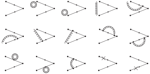
Figure 1: The set of tree-level and one-loop diagrams contributing to the boundary-to-bulk correlation functions $g_{\rm X}^{f_{1}f_{2}}$ and $l_{\rm Y}^{f_{1}f_{2}}$. Fermion propagators are represented by continuous lines, while curly lines represent the gluon propagator. Fermionic counterterms insertions are represented by a cross on a fermion line. Gluon lines not starting from a fermion line originate from the explicit time like link variables in the fermionic boundary fields $\zeta$ and $\bar{\zeta}$, Eqs. (62),(63).

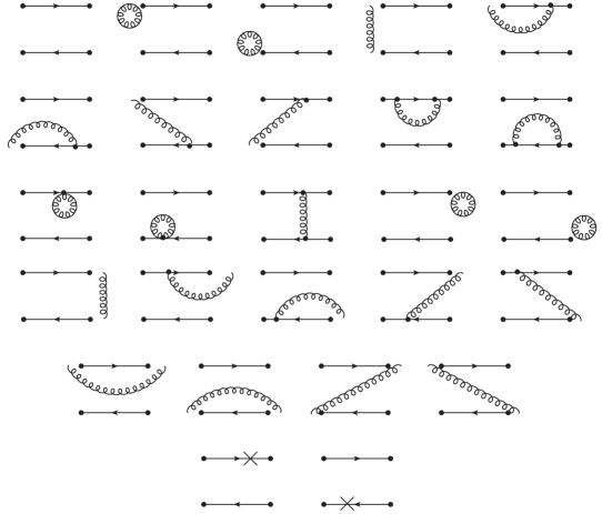
Figure 2: The set of tree-level and one-loop diagrams contributing to the boundary-to-boundary correlation functions $g_{1}^{f_{1}f_{2}}$ and $l_{1}^{f_{1}f_{2}}$.

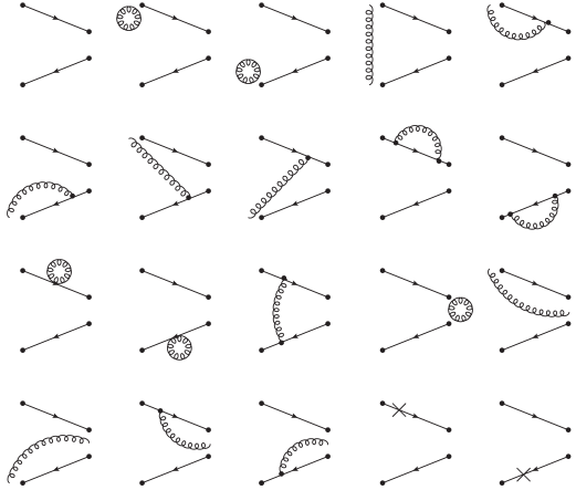
Figure 3: The set of tree-level and one-loop diagrams contributing to the boundary-to-bulk correlation functions involving the point-split vector current, i.e., $g_{\rm\widetilde{V}}^{f_{1}f_{2}}$ and $l_{\rm\widetilde{V}}^{f_{1}f_{2}}$. Note that each diagram in the figure represents the two terms forming the point-split current (88). The two fermion lines do not meet at the vertex due to the point-split nature of the current, and gluons lines may originate from the gauge links that appear in the operator.

5.2 The numerical calculation and checks performed

All terms appearing in (111) and (112) are functions of $a/L$ that can be evaluated numerically by inserting the explicit time-momentum representation of the vertices and propagators into the expressions of each diagram. To this end, we have produced a FORTRAN program for the numerical evaluation of Feynman diagrams both in the standard and chirally rotated SF. Numerical results for each diagram and counterterm have been compared against previous calculations Weisz:private in the case of the standard SF, finding agreement up to rounding errors. For the $\chi$SF we have checked all diagrams for the $g_{\rm X}$ and $l_{\rm Y}$ correlators by an independent FORTRAN program, excluding the ones involving the point-split vector current. A check for the latter has been performed by comparing ratios of correlators to Monte Carlo simulations at small values of the bare coupling, $g_{0}^{2}$, cf. Appendix C. Further confidence in the correctness of our code is gained by the perfect agreement with results in the literature for the current normalization constants (cf. Section 7). We have numerically checked gauge parameter independence for all correlators on small lattices and then performed all subsequent calculations in the Feynman gauge (setting the gauge parameter $\lambda_{0}=1$), in which the gluon propagator for the plaquette action is diagonal. This allows for a considerable speed-up in the numerical computation. A technical point worth noting is that we calculated the fermion propagator for fixed spatial momentum by numerical matrix inversion, as the available analytic result assumes $d_{s}=1$, whereas the correct tree-level value is $d_{s}^{(0)}=1/2$ Sint:2010eh . While it would have been possible to calculate an approximate fermion propagator analytically by single or double insertion of the boundary counterterm, we refrained from doing this as it would prevent a direct comparison with non-perturbative data at finite lattice spacing.

In the remainder of this section we determine the one-loop parameters of the lattice action, $m_{\rm cr}^{(1)}$, $z_{f}^{(1)}$ and $d_{s}^{(1)}$ from this data, and $c_{\rm t}^{(1)}$ is quoted from a separate calculation of the fermion determinant following the lines of ref. Sint:1995ch , as described in Section 8.

5.3 Determination of $m_{\rm cr}^{(1)}$ and $z_{f}^{(1)}$

The determination of $m_{\rm cr}$ and $z_{f}$ is done by solving simultaneously the system of equations consisting of the conditions (75) (with flavours $f_{1}f_{2}=ud$) and (76). Expanding these equations to order $g_{\rm R}^{2}$, we obtain

$$\begin{split}0=&\,\tilde{\partial}_{0}g_{\rm A}^{ud(1,a)}+m_{\rm cr}^{(1)}\tilde{\partial}_{0}g_{{\rm A};m_{0}}^{ud(0)}+z_{f}^{(1)}\tilde{\partial}_{0}g_{{\rm A};z_{f}}^{ud(0)}+d_{s}^{(1)}\tilde{\partial}_{0}g_{{\rm A};d_{s}}^{ud(0)}\\ &\,+\bar{d}_{s}^{(1)}\tilde{\partial}_{0}g_{{\rm A};\bar{d}_{s}}^{ud(0)}+ac_{\rm A}^{(1)}\partial_{0}^{\ast}\partial_{0}g_{\rm P}^{ud(0)},\end{split}$$ (118)

and

$$0=g_{\rm A}^{ud(1,a)}+m_{\rm cr}^{(1)}g_{{\rm A};m_{0}}^{ud(0)}+z_{f}^{(1)}g_{{\rm A};z_{f}}^{ud(0)}+d_{s}^{(1)}g_{{\rm A};d_{s}}^{ud(0)}+\bar{d}_{s}^{(1)}g_{{\rm A};\bar{d}_{s}}^{ud(0)}+ac_{\rm A}^{(1)}\tilde{\partial}_{0}g_{\rm P}^{ud(0)},$$ (119)

where we always assume $x_{0}=T/2$, and $T=L$. The determination of $m_{\rm cr}^{(1)}$ and $z_{f}^{(1)}$ becomes particularly simple when choosing $\theta=0$. Indeed, for this choice, the contributions of the counterterms proportional to $d_{s}$, $\bar{d}_{s}$ and $c_{\rm A}$ vanish. Moreover, for $\theta=0$, the contribution of the counterterm proportional to $z_{f}^{(1)}$ in (119) is constant in $x_{0}$, and hence the derivative $\tilde{\partial}_{0}g_{{\rm A};z_{f}}^{ud(0)}$ in (118) vanishes. The determination of $m_{\rm cr}^{(1)}$ thus becomes independent of $z_{f}^{(1)}$ in this case. For a given lattice size in the range $L/a\in[6,48]$ we then solve the 2 equations and obtain the series

$$m_{\rm cr}^{(1)}(a/L) = -\dfrac{\tilde{\partial}_{0}g_{\rm A}^{ud(1,a)}(L/2)}{\tilde{\partial}_{0}g_{{\rm A};m_{0}}^{ud(0)}(L/2)}\,,$$ (120)

$$z_{f}^{(1)}(a/L) = -\dfrac{g_{\rm A}^{ud(1,a)}(L/2)+m_{\rm cr}^{(1)}(a/L)g_{{\rm A};m_{0}}^{ud(0)}(L/2)}{g_{{\rm A};z_{f}}^{ud(0)}(L/2)}.$$ (121)

From these, we extrapolate to the asymptotic values

$$m_{\rm cr}^{(1)}=\lim_{a/L\rightarrow 0}m_{\rm cr}^{(1)}(a/L),\qquad z_{f}^{(1)}=\lim_{a/L\rightarrow 0}z_{f}^{(1)}(a/L),$$ (122)

following the blocking method described in Bode:1999sm . The values obtained in this way are collected in Table 1 for the fundamental representation of the gauge group. We reproduce the values of $m_{\rm cr}^{(1)}$ available in the literature GonzalezArroyo:1982ts ; Stehr:1982en ; Wholert_desy , as expected, since these asymptotic results only depend on the regularization of the bulk action, and are hence unaffected by the choice of boundary conditions. This is a further strong check on the correctness of our calculation. The values for $z_{f}^{(1)}$, instead, have been calculated here for the first time, cf. Table 1.

	$am_{\rm cr}^{(1)}$	$z_{f}^{(1)}$
$c_{\rm sw}^{(0)}=1$	$-0.2025565(3)\times C_{\rm F}$	$0.16759(1)\times C_{\rm F}$
$c_{\rm sw}^{(0)}=0$	$-0.32571(2)\times C_{\rm F}$	$0.3291(2)\times C_{\rm F}$

Table 1: Results for $am_{\rm cr}^{(1)}$ and $z_{f}^{(1)}$ with and without the clover term, for the fundamental representation of the gauge group.

In order to check the correctness of the determination of $z_{f}^{(1)}$, we recompute it using the following alternative renormalization conditions (again for $x_{0}=T/2$, $T=L$ and $\theta=0$),

$$g_{\rm P}^{uu^{\prime}}=0,\qquad l_{\rm V}^{ud}=0\qquad\textrm{and}\qquad l_{\rm T}^{uu^{\prime}}=0\,,$$ (123)

and the same solution for $m_{\rm cr}^{(1)}$ as before. In each case we obtained an asymptotic value of $z_{f}^{(1)}$ consistent with those in Table 1.

Finally, we calculated the differences $\Delta z_{f}^{(1)}(a/L)$ at finite lattice spacing between $z_{f}^{(1)}(a/L)$ obtained using the condition (76), and that obtained with the conditions (123), i.e.,

$$\Delta z_{f}^{(A)} = \left.z_{f}^{(1)}\right|_{g_{\rm P}^{uu^{\prime}}=0}-\left.z_{f}^{(1)}\right|_{g_{\rm A}^{ud}=0},$$

$$\Delta z_{f}^{(B)} = \left.z_{f}^{(1)}\right|_{l_{\rm T}^{uu^{\prime}}=0}-\left.z_{f}^{(1)}\right|_{g_{\rm A}^{ud}=0},$$ (124)

$$\Delta z_{f}^{(C)} = \left.z_{f}^{(1)}\right|_{l_{\rm V}^{ud}=0}-\left.z_{f}^{(1)}\right|_{g_{\rm A}^{ud}=0}.$$

These are displayed in Figure 4. For $\theta=0$ the only source of cutoff effects in these differences comes from the bulk action, and is completely eliminated by the clover term. Hence, for $c_{\rm sw}^{(0)}=1$ the differences $\Delta z_{f}^{(1)}$ behave as an O($a^{2}$) effect, in contrast to $c_{\rm sw}^{(0)}=0$ for which they behave linearly in $a$, up to possible logarithmic corrections.

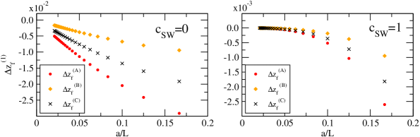
Figure 4: Differences in the value of $z_{f}^{(1)}$ at finite lattice spacing obtained with the different tuning conditions given in Eqs. (76) and (123) (all data for $\theta=0$ and $C_{\rm F}=4/3$).

5.4 Determination of $d_{s}^{(1)}$

The determination of the 1-loop boundary improvement coefficient $d_{s}^{(1)}$ can be obtained by requiring the absence of O($a$) effects at O($g_{\rm R}^{2}$) in some $P_{5}$-even observable. Following a strategy similar to the one used in Luscher:1996vw for the extraction of the boundary improvement coefficient $\tilde{c}_{\rm t}^{(1)}$, we consider the ratio

$$R_{\rm P}(\theta,a/L)=\left.{\left[g_{\rm P}^{ud}(x_{0};\theta,a/L)\right]_{\rm R}\over\left[g_{\rm P}^{ud}(x_{0};0,a/L)\right]_{\rm R}}\right|_{x_{0}=T/2}=R_{\rm P}^{(0)}(\theta,a/L)\left(1+g_{\rm R}^{2}\,r_{\rm P}^{(1)}(\theta,a/L)+{\rm O}(g_{\rm R}^{4})\right),$$ (125)

which has a finite continuum limit, and the tree level ratio, $R_{\rm P}^{(0)}(\theta,a/L)$, is O($a$) improved. The one-loop ratio $r_{\rm P}^{(1)}(\theta,a/L)$ can then be expanded in $a/L$

$$\begin{split}r_{\rm P}^{(1)}(\theta,a/L)=&\left(\left.{g_{\rm P}^{ud(1,a)}\over g_{\rm P}^{ud(0)}}\right|_{\theta}-\left.{g_{\rm P}^{ud(1,a)}\over g_{\rm P}^{ud(0)}}\right|_{\theta=0}\right)+m_{\rm cr}^{(1)}\left(\left.{g_{{\rm P};m_{0}}^{ud(0)}\over g_{\rm P}^{ud(0)}}\right|_{\theta}-\left.{g_{{\rm P};m_{0}}^{ud(0)}\over g_{\rm P}^{ud(0)}}\right|_{\theta=0}\right)\\ &+z_{f}^{(1)}\left(\left.{g_{{\rm P};z_{f}}^{ud(0)}\over g_{\rm P}^{ud(0)}}\right|_{\theta}-\left.{g_{{\rm P};zf}^{ud(0)}\over g_{\rm P}^{ud(0)}}\right|_{\theta=0}\right)+d_{s}^{(1)}\left.{g_{{\rm P};d_{s}}^{ud(0)}\over g_{\rm P}^{ud(0)}}\right|_{\theta},\\ =&\;r_{\rm P}^{(1)}(\theta,0)+\frac{a}{L}\left(r_{1}+d_{s}^{(1)}\frac{L}{a}\left.{g_{{\rm P};d_{s}}^{ud(0)}\over g_{\rm P}^{ud(0)}}\right|_{\theta}\right)+{\rm O}(a^{2}),\end{split}$$ (126)

where the constant $r_{1}$ is the coefficient of the O($a$) effect in $r_{\rm P}^{(1)}(\theta,a/L)$ in the absence of the $d_{s}$-counterterm. Hence, the condition that $r_{\rm P}^{(1)}(\theta,a/L)$ be O($a$) improved leads to the equation

$$d_{s}^{(1)}=-r_{1}\times\left[\lim_{a/L\rightarrow 0}\left(\dfrac{L}{a}\left.{g_{{\rm P};d_{s}}^{ud(0)}\over g_{\rm P}^{ud(0)}}\right|_{\theta}\right)\right]^{-1}\,.$$ (127)

We have analysed the sequence of values for $L/a=6,8,\ldots,48$ with the blocking procedure of ref. Bode:1999sm . Besides $\theta=0.5$ we have produced further data for the set of values $\theta=0.1,0.25,0.75$ and $1.0$. In the case of the O($a$) improved data $c_{\rm sw}^{(0)}=1$ we also considered analogous ratios to Eq. (125) using $l_{\rm A}^{ud}(x_{0})$ and the boundary-to-boundary correlation functions $g_{1}^{ud}$ and $l_{1}^{ud}$. Consistent numerical results were obtained and we quote

$$d_{s}^{(1)}=\left\{\begin{array}[]{cl}-0.0006(3)\times C_{\rm F},&c_{\rm sw}^{(0)}=1\,,\\ -0.0184(5)\times C_{\rm F},&c_{\rm sw}^{(0)}=0\,.\\ \end{array}\right.$$ (128)

Note that this consistency indirectly verifies automatic O($a$) improvement, as it demonstrates the irrelevance at O($a$) of both the counterterm proportional to $\bar{d}_{s}$ (which was omitted) and of the SW-term in the case of the unimproved Wilson fermion data.

5.5 Determination of $c_{\rm t}^{(1)}$

In order to obtain the complete set of $\chi$SF action parameters to order $g_{0}^{2}$, we would also like to compute the one-loop coefficient,

$$c_{\rm t}^{(1)}=c_{\rm t}^{(1,0)}+{N_{\rm f}}c_{\rm t}^{(1,1)},$$ (129)

for the lattice $\chi$SF regularization. However, $c_{\rm t}$ multiplies a gluonic counterterm, so that the fermionic correlation functions at one-loop order are only sensitive to its tree-level value, $c_{\rm t}^{(0)}=1$. We thus consider a gluonic observable, the SF coupling, $\bar{g}^{2}(L)$, defined as the response coefficient to a chromo-electric background field in ref. Luscher:1992an . Expanding in the bare coupling,

$$\bar{g}^{2}(L)=g_{0}^{2}+p_{1}(L/a)g_{0}^{4}+{\rm O}(g_{0}^{6}),$$ (130)

the logarithmically divergent one-loop coefficient, $p_{1}(L/a)$, decomposes into a purely gluonic, and a fermionic contribution,

$$p_{1}(L/a)=p_{1,0}(L/a)+{N_{\rm f}}\,p_{1,1}(L/a).$$ (131)

For gauge groups SU(2) and SU(3) the gluonic coefficient $p_{1,0}$ was first computed in Luscher:1992an ; Luscher:1993gh and the fermionic part, $p_{1,1}$, in ref. Sint:1995ch , for fermions in the fundamental representation and with standard SF boundary conditions. Given the nature of these calculations with a non-trivial gauge background field, it is not obvious how these results depend on the number of colours, $N$, and the fermion representation. This dependence has been worked out in ref. Hietanen:2014lha where the results are given for general $N$ and SU($N$) group constants. In particular the gluonic coefficient, first computed for SU(3) in ref. Luscher:1993gh , takes the form,

$$c_{\rm t}^{(1,0)}=-0.08900(5)=\left[-0.0316483(4)\times N+\dfrac{0.017852(13)}{N}\right]_{N=3},$$ (132)

and is, to this order, independent of the fermion regularization. The analysis of $p_{1,1}(L/a)$ nicely illustrates some of the main points of this paper and is left to Section 8. We here just quote the result of this analysis for fermions in the fundamental representation,

$$c_{\rm t}^{(1,1)}=\left\{\begin{array}[]{cll}-0.006610(5),&\text{$\chi$SF},&c_{\rm sw}^{(0)}=0,\\ \phantom{-}0.006890(5),&\text{$\chi$SF},&c_{\rm sw}^{(0)}=1,\\ \phantom{-}0.019141(2),&\phantom{\chi}\text{SF},&c_{\rm sw}^{(0)}=1.\\ \end{array}\right.$$ (133)

The value for the standard SF is in perfect agreement with ref. Sint:1995ch . According to ref. Hietanen:2014lha , for a general fermion representation $R$ these numbers need to be scaled by $T(R)/T(F)$, where $T(R)$ refers to the normalisation of the trace of two (hermitian) SU($N$)-generators in the representation $R$.

6 Perturbative tests

Having determined the action parameters to O($g_{0}^{2}$) we may now test the theoretical expectations discussed in Sect. 4 to this order in perturbation theory. This section describes our tests of the boundary conditions, the mechanism of automatic O($a$) improvement, the restoration of flavour symmetry and a direct comparison between SF and $\chi$SF observables.

6.1 Boundary conditions

On the lattice boundary conditions are not so much imposed as implicitly encoded by the structure of the action near the boundary. Testing whether the boundary conditions are satisfied (up to cutoff effects) is therefore not trivial. Considering the first ratios of Eq. (79) at $x_{0}=T/2$, we expand perturbatively,

$$R_{\rm X,-}^{g,f_{1}f_{2}}=R_{\rm X,-}^{g,f_{1}f_{2}(0)}+g_{\rm R}^{2}R_{\rm X,-}^{g,f_{1}f_{2}(1)}+{\rm O}(g_{\rm R}^{4}),$$ (134)

with the tree-level and one-loop terms given by

$$R_{\rm X,-}^{g,f_{1}f_{2}(0)}=\dfrac{g_{{\rm X},-}^{f_{1}f_{2}(0)}}{g_{\rm X}^{f_{1}f_{2}(0)}}\,,\qquad R_{\rm X,-}^{g,f_{1}f_{2}(1)}=R_{\rm X,-}^{g,f_{1}f_{2}(0)}\left\{\dfrac{g_{{\rm X},-}^{f_{1}f_{2}(1)}}{g_{{\rm X},-}^{f_{1}f_{2}(0)}}-\dfrac{g_{\rm X}^{f_{1}f_{2}(1)}}{g_{\rm X}^{f_{1}f_{2}(0)}}\right\}\,.$$ (135)

Analogous expressions are obtained for other ratios in Eq. (79), and for the corresponding ratios of standard SF correlation functions.

Using these definitions we compute the tree-level and one-loop terms in (134) for all the $P_{5}$-even boundary-to-bulk correlation functions, for $c_{\rm sw}^{(0)}=1$ and for $\theta=0,0.5$, and their standard SF counterparts. The tree-level ratios vanish exactly when $\theta=0$, both in the $\chi$SF and in the standard SF. For $\theta=0.5$ instead, the tree-level ratios are non-zero at finite lattice spacing, and vanish at a rate of O($a^{2}$), cf. Figure 5. We find that the size of the cutoff effects in both set-ups is comparable at tree-level. Note that the tree-level correlators do not depend on $c_{\rm sw}^{(0)}$, due to our choice of trivial gauge background field.

In order to evaluate the same ratios at one-loop order, we insert the series $m_{\rm cr}^{(1)}(a/L)$ and $z_{f}^{(1)}(a/L)$ obtained from $g^{ud}_{\rm A}$ at finite $L/a$ and for $\theta=0$. The convergence to the continuum limit of the ratios is displayed in Figure 6. We note that the ratios are very small for the $\chi$SF already at the coarsest lattices, both for $\theta=0$ and $0.5$. In the first case, cutoff effects are particularly suppressed, and seem to approach zero faster than O($a^{2}$) (top-left panel of Figure 6), whereas the data for $\theta=0.5$ shows the O($a^{2}$) continuum approach that one might have expected (top-right panel of Figure 6). For the standard SF the ratios at one-loop, although still small, are an order of magnitude larger than their $\chi$SF counterparts (see bottom panels of Figure 6). In summary, we note that all the ratios considered approach zero in the continuum limit, at least with a rate of O($a^{2}$). This confirms that the boundary conditions are correctly implemented to one-loop order of perturbation theory.

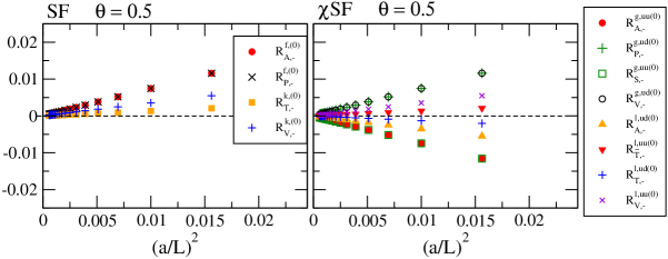
Figure 5: Tree-level ratios (135) between correlation functions defined with reverted projectors and correct projectors, respectively. Ratios for both standard SF (left panel) and $\chi$SF (right panel) boundary conditions are shown for $\theta=0.5$.

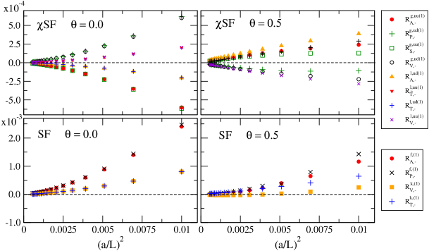
Figure 6: One-loop ratios (135) between correlation functions defined with reverted and correct projectors, respectively, for $c_{\rm sw}=1$ and both $\theta=0$ and $0.5$. The factor $C_{\rm F}=4/3$ is included. The ratios for the $\chi$SF are displayed in the upper panels, while those for the SF are shown in the lower panels (note the scale difference).

6.2 Automatic O($a$) improvement

As explained in Subsection 4.2 we may test automatic O($a$) improvement either by confirming the O($a^{2}$) continuum approach of $P_{5}$-even observables, or by showing that the associated bulk O($a$) counterterm contributions, or, more generally, $P_{5}$-odd correlations, are pure O($a$) effects. Several examples of the former will appear below, where the absence of cutoff effects linear in $a$ is observed. We here focus on the $P_{5}$-odd correlations functions, which are the ones translating to $f_{\rm S},f_{\rm V}$ or $k_{\rm A},k_{\rm\widetilde{T}}$ according to our dictionary of Section 2. Among those we omit the ones which vanish identically, Eq. (67), which leaves us with non-trivial tests of automatic O($a$) improvement to be performed for

$$g_{\rm A}^{ud},g_{\rm P}^{uu^{\prime}},l_{\rm V}^{ud},l_{\rm T}^{uu^{\prime}},$$ (136)

as well as the derivatives

$$\tilde{\partial}_{0}g_{\rm P}^{uu^{\prime}},\tilde{\partial}_{0}l_{\rm V}^{ud},\tilde{\partial}_{0}l_{\rm T}^{uu^{\prime}},$$ (137)

which also appear as O($a$) counterterms to the $P_{5}$-even correlation functions $g_{\rm A}^{uu^{\prime}}$, $l_{\rm T}^{ud}$ and $l_{\rm V}^{uu^{\prime}}$, respectively (cf. Appendix A).

We first choose data at $\theta=0$, set $x_{0}=T/2$ and insert the series Eqs. (120),(121) for $m_{\rm cr}^{(1)}$ and $z_{f}^{(1)}$. For $\theta=0$, all $P_{5}$-odd correlation functions at tree-level vanish identically already at finite lattice spacing. At one-loop order, we focus on the correlation functions in Eq. (136), where $g_{\rm A}^{ud}(T/2)=0$ holds by definition, as this is our tuning condition for $z_{f}$. The remaining ones are shown in Figure 7 for both $c_{\rm sw}^{(0)}=0$ (left panel) and $c_{\rm sw}^{(0)}=1$ (right panel). While non-zero at finite lattice spacing, all these $P_{5}$-odd correlation functions do indeed vanish in the continuum limit, as expected from automatic O($a$) improvement. To understand the faster continuum approach in the case of $c_{\rm sw}^{(0)}=1$, we note that with $\theta=0$ the counterterm insertions $\propto c_{\rm A}^{(1)},c_{\rm V}^{(1)},c_{\rm T}^{(1)}$ vanish,

$$\tilde{\partial}_{0}g_{\rm P}^{(0)}(x_{0})|_{\theta=0}=\tilde{\partial}_{0}l_{\rm T}^{(0)}(x_{0})|_{\theta=0}=\tilde{\partial}_{0}l_{\rm V}^{(0)}(x_{0})|_{\theta=0}=0\,,$$ (138)

and similarly the contributions $\propto\bar{d}_{s}^{(1)}$,

$$g_{{\rm X};\bar{d}_{s}}^{(0)}(x_{0})|_{\theta=0}=l_{{\rm Y};\bar{d}_{s}}^{(0)}(x_{0})|_{\theta=0}=0.$$ (139)

The same holds for the $d_{s}$-counterterm. However, both this and the $c_{\rm t}$-counterterm are $P_{5}$-even so that their contribution would anyway be at most an O($a^{2}$) effect. Hence, the only relevant counterterm for O($a$) improvement of these observables is the Sheikholeslami-Wohlert term and its inclusion thus changes the rate of the approach to the continuum limit from O($a$) to O($a^{2}$). As an aside we remark that this observation could be used to determine $c_{\rm sw}^{(0)}$ and thus provides a perturbative example for the kind of O($a$) improvement conditions that can be obtained from the $\chi$SF.

Passing to data for $\theta=0.5$ and $c_{\rm sw}^{(0)}=1$, the $P_{5}$-odd correlation functions are found to vanish in the continuum limit, both at the tree- and one-loop level, with a rate of O($a$) as should be expected (cf. Figure 8). In this case the vanishing of $g_{\rm A}^{ud}(T/2)$ is non-trivial as we obtain $z_{f}$ from data at $\theta=0$. In conclusion, we confirm that $P_{5}$-odd observables are indeed pure lattice artefacts, and confirm that automatic O($a$) improvement works out as theoretically expected.

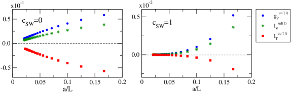
Figure 7: Vanishing $P_{5}$-odd correlation functions at one-loop order, calculated for $c_{\rm sw}=0$ (left panel), $c_{\rm sw}=1$ (right panel) and for $\theta=0$. The series for $m_{\rm cr}^{(1)}(a/L)$ (120) and $z_{f}^{(1)}(a/L)$ (121) have been inserted and $C_{\rm F}=4/3$ (note the scale difference between the panels).

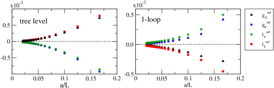
Figure 8: Vanishing $P_{5}$-odd correlation functions for $\theta=0.5$ both at tree-level (left panel) and at one-loop order with $c_{\rm sw}^{(0)}=1$ (right panel). The series for $m_{\rm cr}^{(1)}(a/L)$ (120) and $z_{f}^{(1)}(a/L)$ (121) have been used and the group factors have been set to $N=3$ and $C_{\rm F}=4/3$, respectively.

6.3 Flavour symmetry restoration

In order to check if flavour symmetry is restored in the continuum limit, we consider the relations between boundary-to-boundary correlation functions with different flavour content. Taking the ratios in Eq. (81) and expanding them to order $g_{\rm R}^{2}$,

$$R_{g,l}=R_{g,l}^{(0)}+g_{\rm R}^{2}\,R_{g,l}^{(1)}+{\rm O}(g_{\rm R}^{4}),$$ (140)

we should find that the tree-level coefficients,

$$R_{g}^{(0)}={g_{1}^{uu^{\prime}(0)}\over g_{1}^{ud(0)}},\qquad R_{l}^{(0)}={l_{1}^{uu^{\prime}(0)}\over l_{1}^{ud(0)}},$$ (141)

approach unity, whereas the one-loop coefficients,

$$R_{g}^{(1)}=R_{g}^{(0)}\left\{{g_{1}^{uu^{\prime}(1)}\over g_{1}^{uu^{\prime}(0)}}-{g_{1}^{ud(1)}\over g_{1}^{ud(0)}}\right\},\qquad R_{l}^{(1)}=R_{l}^{(0)}\left\{{l_{1}^{uu^{\prime}(1)}\over l_{1}^{uu^{\prime}(0)}}-{l_{1}^{ud(1)}\over l_{1}^{ud(0)}}\right\},$$ (142)

should vanish in the continuum limit. Computing these coefficients for $c_{\rm sw}^{(0)}=1$ and $0$ and for $\theta=0$ and $0.5$, we find that the ratios at tree-level are exactly $R_{g}^{(0)}=R_{l}^{(0)}=1$ for all values of $L/a$ and independently of $\theta$. The one-loop coefficients $R_{g}^{(1)}$ and $R_{l}^{(1)}$ are non-zero at finite lattice spacing, but vanish as $a/L\rightarrow 0$, thus confirming the restoration of flavour symmetry. The counterterm insertions proportional to $d_{s}^{(1)}$ vanish exactly in this ratio rendering this counterterm irrelevant not only at O($a$) (as expected from the discussion in Subsect.  4.3) but to all orders in $a$. Somewhat surprisingly, the same statement holds for the counterterm insertions proportional to $m_{\rm cr}^{(1)}$ and $z_{f}^{(1)}$, so that the choice of the critical mass or the precise definition of $z_{f}$ become irrelevant, too. The results for the coefficients $R_{g}^{(1)}$ and $R_{l}^{(1)}$ are displayed in Figure 9 for $c_{\rm sw}^{(0)}=1$. The behaviour for both values of $\theta$ is very similar and the continuum limit is approached at an even faster rate than the expected O($a^{2}$).

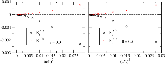
Figure 9: One-loop ratios $R_{g}^{(1)}$ and $R_{l}^{(1)}$, Eq. (142), as a function of $(a/L)^{2}$ for $c_{\rm sw}^{(0)}=1$. The factor $C_{\rm F}=4/3$ has been included.

6.4 Direct comparison SF vs. $\chi$SF

As explained in Sect. 4.5 the bare fermionic boundary source fields being different represents an obstacle when directly comparing fermionic correlation functions between the SF and $\chi$SF. We are thus led to consider (double) ratios where the boundary source renormalization factors $Z_{\zeta}$ are cancelled separately for SF and $\chi$SF observables, e.g.

$$R_{\rm A}=\Bigg{[}{{[g_{\rm A}^{uu^{\prime}}]_{\rm R}}\over{\sqrt{[g_{1}^{uu^{\prime}}]_{\rm R}}}}\Bigg{]}\times\Bigg{[}{{[f_{\rm A}]_{R}}\over{\sqrt{[f_{1}]_{R}}}}\Bigg{]}^{-1},\qquad R_{\rm P}=\Bigg{[}{{[g_{\rm P}^{ud}]_{\rm R}}\over{\sqrt{[g_{1}^{ud}]_{\rm R}}}}\Bigg{]}\times\Bigg{[}{{[f_{\rm P}]_{\rm R}}\over{\sqrt{[f_{1}]_{\rm R}}}}\Bigg{]}^{-1}\,,$$ (143)

where we have suppressed the $x_{0}$-dependence. Such ratios are expected to approach 1 in the continuum limit, and similar ratios could be obtained from the $k$- and $l$-functions, with vector and tensor bilinears. In fact, up to a tree-level factor, all these double ratios correspond to ratios between $Z$-factors defined in SF schemes, cf. Eq. (102). Since the bare fermion bilinear operators and the bulk lattice regularization here are taken to be the same for SF and $\chi$SF, the renormalization factors must be equal up to cutoff effects. For these effects to be reduced to O($a^{2}$) full Symanzik improvement of the action and fields is required on the SF side. Note that this requirement imposes the use of the improved action also for the $\chi$SF. Furthermore, one needs to implement boundary O($a$) improvement for the $\chi$SF by tuning $d_{s}$ and $c_{\rm t}$. Automatic O($a$) improvement of the $\chi$SF then ensures that the bulk O($a$) counterterms to the fields as well as the $P_{5}$-odd boundary counterterm $\propto\bar{d}_{s}$ do not contribute at O($a$) and may be omitted.

To study the continuum approach for $R_{\rm A}$ and $R_{\rm P}$ to O($g_{\rm R}^{2}$), we expand the ratios in the coupling,

$$R_{\rm X}=R_{\rm X}^{(0)}+g_{\rm R}^{2}\,R_{\rm X}^{(1)}+{\rm O}(g_{\rm R}^{4}),$$ (144)

with the tree-level terms given by

$$R_{\rm X}^{(0)}={g_{\rm X}^{(0)}\over\sqrt{g_{1}^{(0)}}}\cdot{\sqrt{f_{1}^{(0)}}\over f_{\rm X}^{(0)}},$$ (145)

and the 1-loop terms,

$$R_{\rm X}^{(1)}=R_{\rm X}^{(0)}\left\{{g_{\rm X}^{(1)}\over g_{\rm X}^{(0)}}-{f_{\rm X}^{(1)}\over f_{\rm X}^{(0)}}-{1\over 2}\left({g_{1}^{(1)}\over g_{1}^{(0)}}-{f_{1}^{(1)}\over f_{1}^{(0)}}\right)\right\}.$$ (146)

Looking at data for $x_{0}=T/2$ and $\theta=0$, the tree-level coefficients $R_{\rm A}^{(0)}$ and $R_{\rm P}^{(0)}$ are exactly 1 even at finite $L/a$. For $\theta\neq 0$, $R_{\rm P}^{(0)}$ is still exactly 1, whereas $R_{\rm A}^{(0)}$ shows a small deviation from 1 which apparently vanishes even faster than O($a^{2}$) (see left panel of Figure 10). The one-loop terms $R_{\rm A}^{(1)}$ and $R_{\rm P}^{(1)}$ calculated at $c_{\rm sw}^{(0)}=1$, $\theta=0$ and $\theta=0.5$ are displayed in the right panel of Figure 10. Again we have inserted the finite $a/L$ estimates of $m_{\rm cr}^{(1)}$ (120) and of $z_{f}^{(1)}$ (121). Boundary O($a$) improvement by the $d_{s}$- and $\tilde{c}_{\rm t}$-counterterms, respectively, has been implemented. Furthermore, for $\theta=0.5$, the correlation function $f^{(1)}_{\rm A}$ receives a contribution from the operator improvement counterterm proportional to $c_{\rm A}$, which vanishes for $\theta=0$. We thus also consider $f^{(1)}_{\rm A}$ with the improved axial current $A_{\rm I}$ and label the corresponding ratio of correlation functions as $R_{\rm A_{I}}^{(1)}$. In all cases considered, the one-loop ratios $R_{\rm X}^{(1)}$ converge to 0, thus confirming the expectation of universality. Furthermore, the convergence rate is found to be O$(a^{2})$ provided O($a$) improvement is correctly implemented at the boundaries and in the bulk for the action and the SF correlation functions. Again, this indirectly confirms automatic O($a$) improvement, as the omitted $P_{5}$-odd counterterms $\propto\bar{d}_{s}$ and $\propto c_{\rm A}$ on the $\chi$SF side are not required.

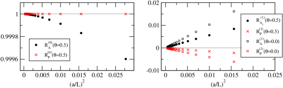
Figure 10: Ratios $R_{\rm A}$ and $R_{\rm P}$ at tree-level (left panel) and 1-loop (right panel) calculated for $c_{\rm sw}^{(0)}=1$ and $C_{\rm F}=4/3$.

7 Applications based on universality

In this section we now assume universality and demonstrate the determination of scale independent renormalization factors like $Z_{\rm A}$ or $Z_{\rm V}$, which are traditionally obtained from chiral and flavour Ward identities, respectively. We then take another look at SF schemes for the pseudo-scalar and tensor densities, and study both the renormalization factors and the associated step-scaling functions.

7.1 Scale-independent renormalization factors

We now consider the ratios of Subsect. 4.4, which should yield the scale independent factors $Z_{\rm A}$ and $Z_{\rm V}$ and the scale independent ratios $Z_{\rm P}/Z_{\rm S}$ and $Z_{\rm T}/Z_{\rm\widetilde{T}}$, up to cutoff effects of order $a^{2}$. Taking for example $R^{g}_{\rm V\tilde{V}}$, Eq. (91), we write the perturbative expansion,

$$R^{g}_{\rm V\widetilde{V}}=R^{g(0)}_{\rm V\widetilde{V}}+g_{\rm R}^{2}R^{g(1)}_{\rm V\widetilde{V}}+{\rm O}(g_{\rm R}^{4})\,.$$ (147)

We set $x_{0}=T/2$ and $T=L$ and then expect the tree-level term to approach unity with O($a^{2}$) corrections and we find this is indeed the case. Focusing on the one-loop contribution, we simplify notation by writing

$$R^{g(1)}_{\rm V\widetilde{V}}=Z_{\rm V}^{g(1)}(L/a),$$ (148)

and similarly for the other estimators of Subsect. 4.4, including those which yield ratios of $Z$-factors, e.g.

$$R^{g(1)}_{\rm PS}=[Z_{\rm P}/Z_{\rm S}]^{(1)}(L/a),$$ (149)

and the superscript $g$ or $l$ referring to the $g_{\rm X}$ or $l_{\rm Y}$ correlation functions is only used when a confusion is possible. Note that, besides the $P_{5}$-odd $\bar{d}_{s}$-counterterm, we also omit the $d_{s}$-counterterm at one-loop order: for $\theta=0$ it vanishes exactly, however, in general it is expected to be irrelevant for the O($a$) improvement of such ratios and will at most cause additional O($a^{2}$) effects (cf. Section 4). We have verified this expectation explicitly by studying the combination of $d_{s}$-counterterm insertions entering the one-loop $Z$-factors. In the case of the vector current normalization constants this combination is even found to vanish exactly.

Following Symanzik’s analysis of cutoff effects, one expects that the asymptotic behaviour for $a/L\rightarrow 0$ is described by,

$$Z_{\rm X}^{(1)}(L/a)\sim\sum_{n=0}^{\infty}\left[r_{{\rm X},n}+s_{{\rm X},n}\ln(L/a)\right](a/L)^{n}.$$ (150)

The coefficient $r_{\rm X,0}$ defines the finite asymptotic value $Z_{\rm X}^{(1)}$. For scale independent renormalization constants, the coefficient multiplying the logarithmic divergence must be zero i.e. $s_{\rm X,0}=0$. All subsequent coefficients in Eq. (150) describe the cutoff effects in $Z_{\rm X}^{(1)}(L/a)$. The term linear in $a/L$ should be absent according to the discussion in Subsect. 4.4 regarding the boundary O($a$) effects. The term proportional to $s_{{\rm X},1}$ is $0$ provided that O($a$) effects are absent in the bulk.

We obtain the first asymptotic coefficients in (150) following the blocking procedure described in Bode:1999sm . For all cases we confirm that the coefficients $s_{{\rm X},0},r_{{\rm X},1}$ and $s_{{\rm X},1}$ are compatible with zero up to at least 5 decimal digits. Assuming these to be zero in the subsequent analysis, we can then easily extract the asymptotic values $r_{{\rm X},0}$. The results are collected in Table 2.

	$c_{\rm sw}=1$	$c_{\rm sw}=0$
$Z_{\rm A}^{(1)}$	$-0.116458(2)$	$-0.133375(2)$
$Z_{\rm V}^{(1)}$	$-0.129430(2)$	$-0.174085(2)$
$\left[Z_{\rm P}/Z_{\rm S}\right]^{(1)}$	$-0.025944(3)$	$-0.081420(3)$

Table 2: One-loop values of the scale-independent renormalization factors of fermion bilinears for O($a$) improved and unimproved Wilson fermions in QCD ($C_{\rm F}=4/3$). Values for general $N$ can be obtained by multiplying the quoted numbers by $(3/4)\times C_{\rm F}$.

Within the quoted errors the asymptotic values $Z_{\rm V}^{(1)}$ and $Z_{\rm A}^{(1)}$ calculated using the $g$- and the $l$-functions are in agreement with each other. We also found agreement with the literature Gabrielli:1990us ; Martinelli:1982mw ; Martinelli:1983be ; Meyer:1983ds ; Groot:1983ng for all renormalization factors, indicating that the method described in Subsection 4.4 for defining finite renormalization constants is well-founded.

7.1.1 Lattice artefacts

Next, we consider the cutoff effects in the finite renormalization factors to O($g_{0}^{2}$) in perturbation theory. At tree-level and one-loop order we define the difference between a given renormalization constant at finite lattice spacing and its asymptotic value, i.e.,

$$\delta Z^{(i)}_{\rm X}(L/a)=Z_{\rm X}^{(i)}(L/a)-Z_{\rm X}^{(i)},\quad i=0,1.$$ (151)

In view of non-perturbative applications we will focus on the case of O($a$) improved Wilson fermions and set $c_{\rm sw}^{(0)}=1$.

At tree-level, all renormalizaton constants are unity, $Z_{\rm X}^{(0)}=1$. For the particular choice of $\theta=0$ this is also true at finite lattice spacing, i.e. $Z_{\rm X}^{(0)}(L/a)=1$, and hence the cutoff effects vanish exactly, $\delta Z_{\rm X}^{(0)}(L/a)=0$ for all $a/L$. For $\theta=0.5$, the tree-level cutoff effects $\delta Z_{\rm V}^{g(0)}$ and $\delta Z_{\rm A}^{g(0)}$ are numerically around $0.01$ for $L/a=6$ and vanish at a rate $\propto a^{2}$. In all other cases (including $\delta Z_{\rm V}^{l(0)}$ and $\delta Z_{\rm A}^{l(0)}$) the cutoff effects are numerically much smaller and also vanish at a higher rate than the expected O($a^{2}$).

The one-loop cutoff effects in $Z_{\rm V}$ and $Z_{\rm A}$ are shown in Figure 11 for $\theta=0$ and $0.5$. We study the cutoff effects obtained by using the asymptotic values of $m_{\rm cr}^{(1)}$ and $z_{f}^{(1)}$ (cf. Table 1) in the expansions of $Z_{\rm V}$ and $Z_{\rm A}$, and also those obtained using the values $m_{\rm cr}^{(1)}(a/L)$ and $z_{f}^{(1)}(a/L)$ at finite $L/a$ and for $\theta=0$ from Eqs. (120),(121). The latter are denoted $\delta Z_{\rm X}^{(1)}$, whereas the former are labelled $\delta Z_{\rm X,as}^{(1)}$. The qualitative picture is similar to that observed at tree-level. Cutoff effects associated to the definitions $Z_{\rm V}^{l}$ and $Z_{\rm A}^{l}$ are always very small even for the smallest lattices, in contrast to the definitions $Z_{\rm V}^{g}$ and $Z_{\rm A}^{g}$ where we observe considerably larger but still rather small effects. An interesting observation is that the insertion of the mass counterterm causes an O(1) effect on $Z_{\rm V}^{g}$ and $Z_{\rm A}^{g}$, whereas it is suppressed by a further power of $a/L$ for $Z_{\rm V}^{l}$ and $Z_{\rm A}^{l}$. The O(1) behaviour is expected since the insertion of the $P_{5}$-odd mass counterterm into the $P_{5}$-even observables combines a power of $a/L$ with a linear divergence $\propto L/a$. What comes as a surprise is the above mentioned additional O($a/L$) suppression, which is also seen for the ratio of tensor densities and in the pseudo-scalar to scalar ratio. Similarly, regarding the $z_{f}$-counterterm we find that its insertion combines to an O($a^{2}$) effect in all cases, except for the vector current where it vanishes exactly. Finally, we recall that the $d_{s}$-counterterm vanishes exactly at $\theta=0$, whereas for $\theta=0.5$ its contributions are at least of O($a^{2}$) and numerically insignificant in all cases, due also to the smallness of $d_{s}^{(1)}$ [cf. Eq. (128)]. Regarding $P_{5}$-odd counterterms, we find no sign of an O($a$) contamination due to the omission of either the $\bar{d}_{s}$-counterterm or the bulk counterterms to the currents. In conclusion, in all cases cutoff effects vanish proportionally to $(a/L)^{2}$, nicely confirming the theoretical expectations expressed in Section 4.

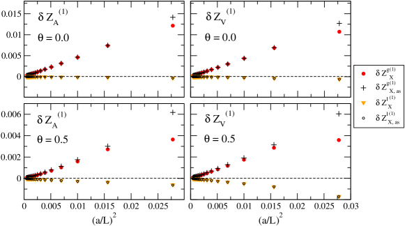
Figure 11: Cutoff effects in $Z_{\rm V}^{(1)}(L/a)$ and $Z_{\rm A}^{(1)}(L/a)$ computed using the different definitions in Eqs. (90)-(92), for $c_{\rm sw}^{(0)}=1$ and $C_{\rm F}=4/3$.

7.2 Scale-dependent renormalization factors

Here we compute to one-loop order in perturbation theory the scale-dependent renormalization factors $Z_{\rm P}$ and $Z_{\rm T}$ in SF schemes, defined by the renormalization conditions, Eqs. (100) and (101). Again we focus on the O($a$) improved action with $c_{\rm sw}^{(0)}=1$ and we first insert the the series Eqs. (120),(121) for $m_{\rm cr}^{(1)}$ and $z_{f}^{(1)}$. Expanding both $Z_{\rm P}$ and $Z_{\rm T}$ in the bare coupling,

$$Z_{\rm X}(g_{0}^{2},L/a)=1+\sum_{k=1}^{\infty}Z_{\rm X}^{(k)}(L/a)g_{0}^{2k},\qquad{\rm X=P,T},$$ (152)

their one-loop coefficients, $Z_{\rm P}^{(1)}(L/a)$ and $Z_{\rm T}^{(1)}(L/a)$, have an asymptotic expansion analogous to Eq. (150), with the finite parts and the coefficients of the logarithmic divergences given by

$$r_{{\rm P},0}=z_{\rm P}^{(1)}(\theta),\qquad s_{{\rm P},0}=-d_{0}=-{6C_{\rm F}\over(4\pi)^{2}},$$ (153)

$$r_{{\rm T},0}=z_{\rm T}^{(1)}(\theta),\qquad s_{{\rm T},0}=\gamma_{\rm T}^{(0)}={2C_{\rm F}\over(4\pi)^{2}}.$$ (154)

Here $-d_{0}$ and $\gamma_{\rm T}^{(0)}$ are the universal one-loop anomalous dimensions of the pseudoscalar and tensor density, respectively. One then expects the coefficients $r_{{\rm X},1}$ and $s_{{\rm X},1}$ to vanish provided that O($a$) lattice artefacts are absent due to both boundary O($a$) improvement ($d_{s}^{(1)}$ and $c_{\rm t}^{(0)}=1$), and automatic O($a$) improvement.

We extract the first asymptotic coefficients in (150) for $Z_{\rm P}^{(1)}(L/a)$ and $Z_{\rm T}^{(1)}(L/a)$ in the way described in Subsect. 7.1. Note that we here omit the $d_{s}$ counterterm: its contribution vanishes in all cases considered except for $Z_{\rm T}^{(1)}(L/a)$ at $\theta=0.5$, where its contribution is so small as to be below our resolution for the O($a$) coefficient $r_{{\rm T},1}$ and can be safely neglected. We then confirm that for all cases the coefficients $r_{{\rm X},1}$ and $s_{{\rm X},1}$ are compatible with zero to least 4 decimal digits. For the $\theta=0.5$ data and to this level of precision we may therefore exclude contributions at O($a$) from the omitted $\bar{d}_{s}$-counterterm, as well as from the bulk O($a$) counterterm $\propto c_{\rm T}$ in the case of the tensor density, thereby providing further evidence for automatic O($a$) improvement.

The coefficients $s_{{\rm P},0}$ and $s_{{\rm T},0}$ agree with their theoretically expected values in Eqs. (153) and (154) to about 5 decimal digits. With this confirmation we set these to their expected values and proceed to extract the asymptotic coefficients $z_{\rm P}^{(1)}$ and $z_{\rm T}^{(1)}$, which we collect in Table 3. The values of $z_{\rm P}^{(1)}$ and $z_{\rm T}^{(1)}$ obtained here are in perfect agreement with the results found in ref. Sint:1998iq and Fritzsch:2015lvo , respectively.

To study the convergence to the continuum we define the subtracted one-loop renormalization constants

$$\Delta_{\rm X}^{(1)}=Z_{\rm X}^{(1)}(L/a)-z_{\rm X}^{(1)}(\theta)-s_{\rm X,0}\ln(L/a)\,,\qquad\text{${\rm X=P,T}$},$$ (155)

where we have now inserted the asymptotic values $m_{\rm cr}^{(1)}$ and $z_{f}^{(1)}$ from table 1. Figure 12 clearly shows the O($a^{2}$) behaviour of the data, with cutoff effects being largest for $\theta=0$.

	$\theta=0$	$\theta=0.5$
$z_{\rm P}^{(1)}$	$-0.119542(1)\times C_{\rm F}$	$-0.092815(1)\times C_{\rm F}$
$z_{\rm T}^{(1)}$	$-0.019852(1)\times C_{\rm F}$	$-0.06270(1)\times C_{\rm F}$

Table 3: One-loop results for the finite parts of the scale dependent renormalization factors $Z_{\rm P}$ and $Z_{\rm T}$, for $c_{\rm sw}^{(0)}=1$ and $\theta=0$ and $0.5$.

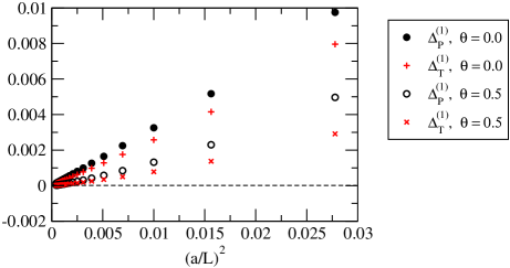
Figure 12: Convergence to the continuum limit of the subtracted one-loop coefficients $\Delta_{\rm P}^{(1)}$ and $\Delta_{\rm T}^{(1)}$, Eq. (155), with $C_{\rm F}=4/3$.

7.2.1 Lattice artefacts in the step scaling functions

For further illustration we look at the respective step-scaling functions for $Z_{\rm P}$ and $Z_{\rm T}$ (cf. Subsection 4.5),

$$\Sigma_{\rm X}(u,a/L)=\left.\frac{Z_{\rm X}(g_{0}^{2},2L/a)}{Z_{\rm X}(g_{0}^{2},L/a)}\right|_{u=\bar{g}^{2}(L)}=1+k_{\rm X}(L/a)\times u+{\rm O}(u^{2}),$$ (156)

where

$$k_{\rm X}(L/a)=Z_{\rm X}^{(1)}(2L/a)-Z_{\rm X}^{(1)}(L/a).$$ (157)

Taking the continuum limit at order $u$ the preceding discussion of the respective $Z$-factors implies the results $k_{\rm P}(\infty)=-d_{0}\ln(2)$ and $k_{\rm T}(\infty)=\gamma_{\rm T}^{(0)}\ln(2)$. To study the approach to these continuum values we define the relative cutoff effects by

$$\delta_{\rm P}(a/L)={k_{\rm P}(L/a)\over k_{\rm P}(\infty)}-1,\qquad\textrm{and}\qquad\delta_{\rm T}(a/L)={k_{\rm T}(L/a)\over k_{\rm T}(\infty)}-1.$$ (158)

These coefficients are shown in figure 13 for $\theta=0$ and $0.5$. Note that we have used the asymptotic values of $m_{\rm cr}^{(1)}$ and $z_{f}^{(1)}$, and we have again omitted the vanishing or (in the case of the tensor density) numerically very small $d_{s}$-counterterm contributions. In all cases the convergence to the continuum limit is dominated by $(a/L)^{2}$ effects already at intermediate lattice sizes. Lattice artefacts turn out to be smaller for $\theta=0.5$ than for $\theta=0$. This difference is particularly pronounced for $\Sigma_{\rm T}$, for which cutoff effects are quite large at $\theta=0$. Note that a similar observation was made for the cutoff effects in $\Sigma_{\rm P}$ when calculated in the standard SF Sint:1998iq .

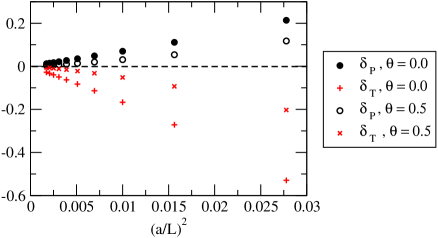
Figure 13: One-loop cutoff effects in the step scaling functions $\Sigma_{\rm P}$ and $\Sigma_{\rm T}$, for $\theta=0$ and $0.5$.

8 The standard SF coupling and $c_{\rm t}$ to one-loop order

We here consider the SF coupling as introduced in Luscher:1992an . Apart from the calculation of the gluonic counterterm $\propto c_{\rm t}$ to order $g_{0}^{2}$, this provides yet another confirmation of universality and automatic O($a$) improvement. With boundary O($a$) improvement in place we also compare the residual lattice effects in the $\chi$SF regularized step scaling functions to the standard SF. In this section we restrict attention to lattice QCD i.e. we assume $N=3$ and fermions in the fundamental representation.

8.1 Analysis of the fermionic one-loop coefficient $p_{1,1}(L/a)$

Taking the expansion of the renormalized SF coupling in $g_{0}^{2}$, Eq. (130), as starting point, the fermionic coefficient $p_{1,1}(L/a)$ can be calculated as in ref. Sint:1995ch , for a given lattice resolution $L/a$ using a recursive evaluation of the determinant for fixed spatial momentum and colour component. The necessary modifications due to $\chi$SF boundary conditions are described in Appendix B. We have written 2 independent FORTRAN codes implementing both SF and $\chi$SF boundary conditions. Perfect agreement (up to rounding errors) was found between both codes using double precision arithmetic. One of the codes was then used to produce data for $p_{1,1}(L/a)$ in quadruple (128 bit) precision arithmetic, for $\theta=\pi/5$, both for $c_{\rm sw}=0$ and $c_{\rm sw}=1$ and for a range of lattice sizes up to $L/a=64$. We have used the asymptotic tree-level values for the fermionic action parameters $z_{f}^{(0)}=1$ and $m_{\rm cr}^{(0)}=0$ and $d_{s}^{(0)}=1/2$, and $\tilde{c}_{\rm t}^{(0)}=1$. The gluonic action parameter is set to $c_{\rm t}=1+g_{0}^{2}c_{\rm t}^{(1)}$, with the fermionic contribution, $c_{\rm t}^{(1,1)}$, as free parameter, to be determined by this calculation. For $a/L\rightarrow 0$ one then expects the data to show the asymptotic behaviour,

$$p_{1,1}(L/a)\sim\sum_{n=0}^{\infty}\left(r_{n}+s_{n}\ln(L/a)\right)(a/L)^{n}.$$ (159)

The logarithmic divergence must be cancelled by the coupling renormalization, implying that its coefficient, $s_{0}$, must be given in terms of the one-loop $\beta$-function. Using the notation

$$b_{0}=b_{0,0}+{N_{\rm f}}b_{0,1},\qquad b_{0,0}=\dfrac{11N}{48\pi^{2}},\qquad b_{0,1}=-\dfrac{1}{24\pi^{2}},$$ (160)

one expects to find Sint:1995ch

$$s_{0}=2b_{0,1}=-\dfrac{1}{12\pi^{2}}\approx-0.008443431966\,.$$ (161)

We extracted the asymptotic coefficients of $p_{1,1}$ from the numerical results following the method described in Bode:1999sm . We first confirmed the expected value for $s_{0}$ for all data sets with a relative precision better than $1$ in $10^{4}$. Then we subtracted $s_{0}\ln(L/a)$ from the data using the analytically expected coefficient for $s_{0}$. This improves the attainable precision for the analysis of the remaining coefficients. The coefficient $r_{0}$ depends on the details of the chosen renormalization scheme for the SF coupling, such as the choice of $\theta$, the aspect ratio $T/L$ or the parameters of the background gauge field. Its value also depends on the regularization through the bare coupling used in the expansion (130). This regularization dependence disappears once the bare coupling is replaced e.g. by the ${\rm\overline{MS\kern-0.50003pt}\kern 0.50003pt}$ coupling (cf. Sint:1995ch ). For $r_{0}$ we find complete agreement with ref. Sint:1995ch , with comparable precision,

$$r_{0}\bigr{|}_{\text{$\chi$SF},\,\theta=\pi/5,\,c_{\rm sw}^{(0)}=1}=-0.0346649(1),\qquad r_{0}\bigr{|}_{\text{$\chi$SF}\,,\theta=\pi/5,\,c_{\rm sw}^{(0)}=0}=-0.0098682(1),$$ (162)

and similarly for data at $\theta=0$, thereby completely confirming the expectation regarding universality.

The coefficients $r_{1}$ and $s_{1}$ are relevant for O($a$) improvement. In particular, with the standard SF, $s_{1}$ was found to vanish only for $c_{\rm sw}^{(0)}=1$, and is therefore related to bulk O($a$) improvement. For the $\chi$SF we thus expect that automatic O($a$) improvement implies $s_{1}=0$, independently of $c_{\rm sw}$. Indeed we find that for all our $\chi$SF data sets $|s_{1}|<10^{-4}$, thus confirming the expectation.

Finally, the coefficient $r_{1}$ is related to boundary O($a$) effects. From the $\theta=\pi/5$ data set with $c_{\rm sw}=1$, we obtain

$$r_{1}\bigr{|}_{\text{$\chi$SF},\,\theta=\pi/5,\,c_{\rm sw}^{(0)}=1}=-2c_{\rm t}^{(1,1)}+0.01378(1).$$ (163)

Requiring the absence of O($a$) effects in the SF coupling at one-loop order means $r_{1}=0$, and thus determines $c_{\rm t}^{(1,1)}$. Note that this result must be independent of $\theta$ or other kinematical parameters. We have checked that the result (163) is reproduced within errors with data at $\theta=0$.

For the $\chi$SF data with $c_{\rm sw}=0$ the corresponding result is

$$r_{1}\bigr{|}_{\text{$\chi$SF},\,\theta=\pi/5,\,c_{\rm sw}^{(0)}=0}=-2c_{\rm t}^{(1,1)}-0.01322(1)\,,$$ (164)

independently of $\theta$. Note that this is in contrast to the standard SF where $r_{1}$ is found to be $\theta$-dependent, indicating that boundary O($a$) improvement in the standard SF cannot be achieved separately from bulk O($a$) improvement. As our data shows, with the $\chi$SF this is indeed possible. More abstractly, this is due to the fact that $P_{5}$-parity distinguishes the even O($a$) boundary counterterms ($\propto c_{\rm t},d_{s}$) from the odd bulk O($a$) counterterm $\propto c_{\rm sw}$.

8.2 Residual cutoff effects in the step-scaling function

In non-perturbative applications the scale evolution of the SF coupling can be traced with the help of the step scaling function (SSF) Luscher:1991wu ,

$$\sigma(u)=\left.\overline{g}^{2}(2L)\right|_{u=\overline{g}^{2}(L)},$$ (165)

which relates the value $u$ of the coupling $\overline{g}^{2}$ at a scale $L$ to its value at a scale $2L$. The lattice version $\Sigma(u,L/a)$ of the step scaling function depends on the details of the regularization and converges to (165) in the continuum limit,

$$\sigma(u)=\lim_{a/L\rightarrow 0}\Sigma(u,a/L).$$ (166)

Both continuum and lattice versions of the SSF are expanded in perturbation theory as,

$$\sigma(u)=u+\sigma_{1}u^{2}+{\rm O}(u^{3}),\qquad\Sigma(u,a/L)=u+\Sigma_{1}(a/L)u^{2}+{\rm O}(u^{3}),$$ (167)

with the 1-loop terms given by

$$\sigma_{1}=2b_{0}\ln(2),\qquad\Sigma_{1}(a/L)=p_{1}(2L/a)-p_{1}(L/a).$$ (168)

We would like to monitor the size of the lattice artefacts in the fermionic contribution to the SSF. Isolating the part $\propto{N_{\rm f}}$,

$$\Sigma_{1}(L/a)=\Sigma_{1,0}(L/a)+{N_{\rm f}}\Sigma_{1,1}(L/a),$$ (169)

and analogously for $\sigma_{1}$, their relative difference,

$$\delta_{1,1}(a/L)=\dfrac{\Sigma_{1,1}(L/a)-\sigma_{1,1}}{\sigma_{1,1}},$$ (170)

is shown in Figure 14 for different levels of improvement. For the $\chi$SF (Figure 14, left panel), the cutoff effects are asymptotically O($a^{2}$) once $c_{\rm t}^{(1,1)}$ is fixed to the correct value (133). Note that boundary O($a$) effects are very different between $c_{\rm sw}=0$ or $1$. Somewhat surprisingly, once these are removed by including the respective values for $c_{\rm t}^{(1,1)}$, the remaining cutoff effects are quite similar for $c_{\rm sw}=0$ and $c_{\rm sw}=1$. For the standard SF (Figure 14, right panel), cutoff effects are essentially zero after O($a$) improvement is implemented in the bulk and at the boundaries. This smallness of the remaining cutoff effects seems to be an accident for this particular choice of background field and kinematical parameters.

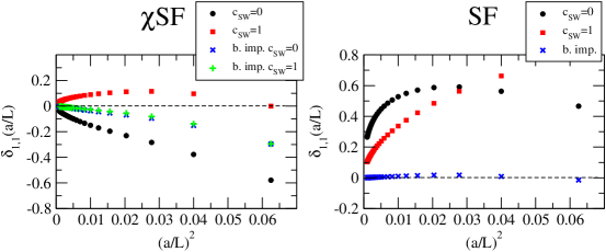
Figure 14: Cutoff effects $\delta_{1,1}$, Eq. (170), for the $\chi$SF (left panel) and the standard SF (right panel). For both the SF and $\chi$SF we show the results with and without clover term. The legend “b. imp.” refers to $c_{\rm t}^{(1,1)}$ being set to the correct values, Eqs. (133), otherwise it is set to zero.

9 Conclusions

In this paper we have defined a complete set of boundary-to-bulk and boundary-to-boundary correlation functions with both $\chi$SF and standard SF boundary conditions. Universality allows to establish a dictionary between both sets which should be applicable to appropriately renormalized correlation functions. We have discussed renormalization and Symanzik O($a$) improvement in terms of these correlation functions. We have then formulated a few theoretical expectations, from the restoration of $\chi$SF boundary conditions, flavour and parity symmetry, to automatic O($a$) improvement, all of which follow from the assumption of a universal continuum limit. We have thus provided the framework for applications and checks of the $\chi$SF both in perturbation theory and beyond.

We have then carried out the perturbative expansion in order to test the theoretical expectations to one-loop order. Based on numerical data for a range of lattice sizes from $L/a=6$ to $L/a=48$ (for both SF and $\chi$SF with and without the SW-term), we have first calculated the action counterterm coefficients $m_{\rm cr}$, $z_{f}$ and $c_{\rm t},d_{s}$ to order $g_{0}^{2}$. The critical mass $m_{\rm cr}$ and the renormalization constant $z_{f}$ are required to restore physical parity and flavour symmetries which are broken at finite lattice spacing. Their determination is thus a pre-condition for any further tests regarding the continuum limit. The counterterms with coefficients $c_{\rm t},d_{s}$ remove O($a$) effects originating from the time boundaries (analogous to $c_{\rm t},\tilde{c}_{\rm t}$ in the standard SF).

Having determined the action to this order we have performed the following tests: first, we have confirmed that the correct boundary conditions are implemented on the lattice. This was done by reversing the projectors in the boundary sources such as to project on the expected Dirichlet components of the fermionic boundary fields. The modified correlation functions were then seen to vanish in the continuum limit, with O($a^{2}$) corrections. For comparison we also looked at the corresponding SF correlation functions, where comparable if larger cutoff effects are observed. Secondly, we have verified that flavour symmetry is restored in the continuum limit. This has been done by checking that ratios of boundary-to-boundary correlation functions with different flavour content converge to unity, such that the continuum relations (44),(45) are satisfied. We then studied ratios of boundary-to-bulk correlation functions which should also approach unity, provided the fermion bilinear operators in the bulk are correctly renormalized. This was confirmed and reproduced a number of results from the literature for ratios of fermion bilinear renormalization constants. Next, we have confirmed the universality between the SF and $\chi$SF set-ups by comparing renormalization constants for the pseudoscalar and tensor densities in SF schemes. Finally, we have checked that the mechanism of automatic O($a$) improvement works as expected. This was done directly, by observing that a set of $P_{5}$-odd correlation functions vanish with a rate of O($a$), and indirectly by observing the absence of O($a$) terms in $P_{5}$-even observables, the cancellation of which would require the O($a$) bulk counterterms. In summary, the perturbative study fully confirms all theoretical expectations and lends further support to the $\chi$SF framework.

With the $\chi$SF firmly established as a new tool, we would like to give a short outlook on current and future applications. With automatic O($a$) improvement in place, any bulk O($a$) effect in physical observables vanishes without the need to tune either the $c_{\rm sw}$ coefficient in the action or any of the operator improvement coefficients. This last property is particularly appealing when studying the renormalization of complicated operators such as 4-fermion or higher-twist operators, where the non-perturbative determination of improvement coefficients is difficult or impractical. A project to determine the step-scaling functions for a complete set of 4-quark operators in lattice QCD is currently in progress Brida:2015b ; Brida:2015c . In this context we remark that, in practice, it seems advantageous to include the clover term in the action, as it drastically reduces the O($a$) ambiguity in the critical mass, even if the axial current in the PCAC relation remains unimproved. This in turn renders the tuning of $z_{f}$ easier and higher order cutoff effects seem strongly reduced, even though the qualitative asymptotic behaviour is expected to remain unchanged. This feature has been observed before in the quenched approximation Sint:2010xy and is now confirmed by our perturbative study.

In forthcoming non-perturbative studies nosotros1:2015 ; nosotros2:2015 we will present further non-perturbative tests of the $\chi$SF and, in particular, results for the non-singlet current normalization constants, $Z_{\rm A}$ and $Z_{\rm V}$ (for preliminary results in ${N_{\rm f}}=2$ lattice QCD cf. Brida:2014zwa ). In this context, perturbation theory allows us to make an informed choice of the parameters and to perturbatively eliminate cutoff effects from the numerical simulation data.

As a further promising application of the $\chi$SF we envisage the determination of the bulk O($a$) improvement coefficients $c_{\rm sw}$, $c_{\rm A},c_{\rm V},c_{\rm T}$. Convenient improvement conditions can be obtained by requiring some $P_{5}$-odd observables to vanish exactly (besides the one used to determine $z_{f}$). A systematic investigation along these lines both in perturbation theory and non-perturbatively is left to future work.

Appendix A Fermion bilinears

We refer to appendix A of ref. Luscher:1996sc for our conventions on the Euclidean $\gamma$-matrices. An over-complete set of fermion bilinear operators is then given by

$$V_{\mu}^{f_{1}f_{2}}(x) =\overline{\psi}_{f_{1}}(x)\gamma_{\mu}\psi_{f_{2}}(x), A_{\mu}^{f_{1}f_{2}}(x) =\overline{\psi}_{f_{1}}(x)\gamma_{\mu}\gamma_{5}\psi_{f_{2}}(x),$$

$$S^{f_{1}f_{2}}(x) =\overline{\psi}_{f_{1}}(x)\psi_{f_{2}}(x), P^{f_{1}f_{2}}(x) =\overline{\psi}_{f_{1}}(x)\gamma_{5}\psi_{f_{2}}(x),$$

$$T_{\mu\nu}^{f_{1}f_{2}}(x) =i\overline{\psi}_{f_{1}}(x)\sigma_{\mu\nu}\psi_{f_{2}}(x), \widetilde{T}_{\mu\nu}^{f_{1}f_{2}}(x) =i\overline{\psi}_{f_{1}}(x)\gamma_{5}\sigma_{\mu\nu}\psi_{f_{2}}(x),$$ (171)

where explicit flavour indices are used instead of the usual labeling through the generators of the flavour group. Over-completeness follows from the fact that only 6 of the tensor densities $T_{\mu\nu}$ and $\widetilde{T}_{\mu\nu}$ are independent due to the identity,

$$\gamma_{5}\sigma_{\mu\nu}=-\frac{1}{2}\varepsilon_{\mu\nu\rho\sigma}\sigma_{\rho\sigma},$$ (172)

with the totally antisymmetric $\varepsilon$-tensor normalized by $\varepsilon_{0123}=1$.

In order to achieve on-shell O($a$) improvement a single counterterm is needed for the bilinear operators in (171), so that,

$$X_{\rm I}^{f_{1}f_{2}}(x)=X^{f_{1}f_{2}}(x)+ac_{\rm X}(g_{0})\delta X^{f_{1}f_{2}}(x).$$ (173)

Here $X^{f_{1}f_{2}}$ is any bilinear operator, while the corresponding O(a) counterterms $\delta X^{f_{1}f_{2}}(x)$ are given by,

$$\delta V_{\mu}^{f_{1}f_{2}}(x) =\tilde{\partial}_{\nu}T_{\mu\nu}^{f_{1}f_{2}}(x), \delta A_{\mu}^{f_{1}f_{2}}(x) =\tilde{\partial}_{\mu}P^{f_{1}f_{2}}(x),$$

$$\delta S^{f_{1}f_{2}}(x) =0, \delta P^{f_{1}f_{2}}(x) =0,$$

$$\delta T_{\mu\nu}^{f_{1}f_{2}}(x) =\tilde{\partial}_{\mu}V_{\nu}^{f_{1}f_{2}}(x)-\tilde{\partial}_{\nu}V_{\mu}^{f_{1}f_{2}}(x), \delta\widetilde{T}_{\mu\nu}^{f_{1}f_{2}}(x) =-\varepsilon_{\mu\nu\rho\sigma}\tilde{\partial}_{\rho}V^{f_{1}f_{2}}_{\sigma}(x).$$ (174)

The coefficients multiplying the O($a$) counterterms are functions of the bare coupling $g_{0}$. In perturbation theory these read:

$$c_{\rm X}(g_{0})=c^{(0)}_{\rm X}+c^{(1)}_{\rm X}g_{0}^{2}+{\rm O}(g_{0}^{4}),$$ (175)

where their tree-level values $c^{(0)}_{\rm X}$ are zero, while the 1-loop values are given by Luscher:1996vw ; Sint:1997jx ; Sint:1997dj

$$c_{\rm V}^{(1)}=-0.01225(1)\times C_{\rm F},\quad c_{\rm A}^{(1)}=-0.005680(2)\times C_{\rm F},\quad c_{\rm T}^{(1)}=c_{\rm\widetilde{T}}^{(1)}=0.00896(1)\times C_{\rm F}.$$ (176)

In the standard SF, the boundary bilinear operators are

$$\mathcal{O}_{5}^{f_{1}f_{2}} =a^{6}\sum_{\mathbf{y,z}}\overline{\zeta}_{f_{1}}(\mathbf{y})P_{+}\gamma_{5}\zeta_{f_{2}}(\mathbf{z}), \mathcal{O}_{5}^{{}^{\prime}f_{1}f_{2}} =a^{6}\sum_{\mathbf{y,z}}\overline{\zeta}^{\prime}_{f_{1}}(\mathbf{y})P_{-}\gamma_{5}\zeta^{\prime}_{f_{2}}(\mathbf{z}),$$

$$\mathcal{O}_{k}^{f_{1}f_{2}} =a^{6}\sum_{\mathbf{y,z}}\overline{\zeta}_{f_{1}}(\mathbf{y})P_{+}\gamma_{k}\zeta_{f_{2}}(\mathbf{z}), \mathcal{O}_{k}^{{}^{\prime}f_{1}f_{2}} =a^{6}\sum_{\mathbf{y,z}}\overline{\zeta}^{\prime}_{f_{1}}(\mathbf{y})P_{-}\gamma_{k}\zeta^{\prime}_{f_{2}}(\mathbf{z}),$$ (177)

where $\mathcal{O}_{5}$ and $\mathcal{O}_{k}$ are the bilinears at $x_{0}=0$, while $\mathcal{O}^{\prime}_{5}$ and $\mathcal{O}^{\prime}_{k}$ are the bilinears at $x_{0}=T$.

Given these definitions, the boundary bilinear operators for the $\chi$SF depend on the flavour structure and are given by

$$\mathcal{Q}_{5}^{uu^{\prime}} =a^{6}\sum_{\mathbf{y,z}}\overline{\zeta}_{u}(\mathbf{y})\gamma_{0}\gamma_{5}Q_{-}\zeta_{u^{\prime}}(\mathbf{z}), \mathcal{Q}_{k}^{uu^{\prime}} =a^{6}\sum_{\mathbf{y,z}}\overline{\zeta}_{u}(\mathbf{y})\gamma_{k}Q_{-}\zeta_{u^{\prime}}(\mathbf{z}),$$

$$\mathcal{Q}_{5}^{dd^{\prime}} =a^{6}\sum_{\mathbf{y,z}}\overline{\zeta}_{d}(\mathbf{y})\gamma_{0}\gamma_{5}Q_{+}\zeta_{d^{\prime}}(\mathbf{z}), \mathcal{Q}_{k}^{dd^{\prime}} =a^{6}\sum_{\mathbf{y,z}}\overline{\zeta}_{d}(\mathbf{y})\gamma_{k}Q_{+}\zeta_{d^{\prime}}(\mathbf{z}),$$

$$\mathcal{Q}_{5}^{ud\phantom{{}^{\prime}}} =a^{6}\sum_{\mathbf{y,z}}\overline{\zeta}_{u}(\mathbf{y})\gamma_{5}Q_{+}\zeta_{d}(\mathbf{z}), \mathcal{Q}_{k}^{ud\phantom{{}^{\prime}}} =a^{6}\sum_{\mathbf{y,z}}\overline{\zeta}_{u}(\mathbf{y})\gamma_{0}\gamma_{k}Q_{+}\zeta_{d}(\mathbf{z}),$$

$$\mathcal{Q}_{5}^{du\phantom{{}^{\prime}}} =a^{6}\sum_{\mathbf{y,z}}\overline{\zeta}_{d}(\mathbf{y})\gamma_{5}Q_{-}\zeta_{u}(\mathbf{z}), \mathcal{Q}_{k}^{du\phantom{{}^{\prime}}} =a^{6}\sum_{\mathbf{y,z}}\overline{\zeta}_{d}(\mathbf{y})\gamma_{0}\gamma_{k}Q_{-}\zeta_{u}(\mathbf{z}),$$ (178)

for the boundary at $x_{0}=0$, and

$$\mathcal{Q}_{5}^{\prime uu^{\prime}} =-a^{6}\sum_{\mathbf{y,z}}\overline{\zeta}^{\prime}_{u}(\mathbf{y})\gamma_{0}\gamma_{5}Q_{+}\zeta^{\prime}_{u^{\prime}}(\mathbf{z}), \mathcal{Q}_{k}^{\prime uu^{\prime}} =\phantom{-}a^{6}\sum_{\mathbf{y,z}}\overline{\zeta}^{\prime}_{u}(\mathbf{y})\gamma_{k}Q_{+}\zeta^{\prime}_{u^{\prime}}(\mathbf{z}),$$

$$\mathcal{Q}_{5}^{\prime dd^{\prime}} =-a^{6}\sum_{\mathbf{y,z}}\overline{\zeta}^{\prime}_{d}(\mathbf{y})\gamma_{0}\gamma_{5}Q_{-}\zeta^{\prime}_{d^{\prime}}(\mathbf{z}), \mathcal{Q}_{k}^{\prime dd^{\prime}} =\phantom{-}a^{6}\sum_{\mathbf{y,z}}\overline{\zeta}^{\prime}_{d}(\mathbf{y})\gamma_{k}Q_{-}\zeta^{\prime}_{d^{\prime}}(\mathbf{z}),$$

$$\mathcal{Q}_{5}^{\prime ud\phantom{{}^{\prime}}} =\phantom{-}a^{6}\sum_{\mathbf{y,z}}\overline{\zeta}^{\prime}_{u}(\mathbf{y})\gamma_{5}Q_{-}\zeta^{\prime}_{d}(\mathbf{z}), \mathcal{Q}_{k}^{\prime ud\phantom{{}^{\prime}}} =-a^{6}\sum_{\mathbf{y,z}}\overline{\zeta}^{\prime}_{u}(\mathbf{y})\gamma_{0}\gamma_{k}Q_{-}\zeta^{\prime}_{d}(\mathbf{z}),$$

$$\mathcal{Q}_{5}^{\prime du\phantom{{}^{\prime}}} =\phantom{-}a^{6}\sum_{\mathbf{y,z}}\overline{\zeta}^{\prime}_{d}(\mathbf{y})\gamma_{5}Q_{+}\zeta^{\prime}_{u}(\mathbf{z}), \mathcal{Q}_{k}^{\prime du\phantom{{}^{\prime}}} =-a^{6}\sum_{\mathbf{y,z}}\overline{\zeta}^{\prime}_{d}(\mathbf{y})\gamma_{0}\gamma_{k}Q_{+}\zeta^{\prime}_{u}(\mathbf{z}),$$ (179)

for the boundary at $x_{0}=T$.

Appendix B One-loop contribution to the SF coupling from fermions in the $\chi$SF

We present a few details on the perturbative calculation of the coefficient $p_{1,1}(L/a)$ in Eqs. (130) and (131) with $\chi$SF boundary conditions. The discussion follows very closely Appendix A of ref. Sint:1995ch , where the coefficient $p_{1,1}(L/a)$ was calculated for the standard SF. The reader will be assumed to be familiar with this reference, as we will adopt much of the notation from there without further notice (in particular we use lattice units $a=1$ and $t=x_{0}$ for Euclidean time).

For definiteness we assume a doublet with ${N_{\rm f}}=2$ flavours. One then has

$$p_{1,1}=\frac{1}{2k}\left.\frac{\partial}{\partial\eta}\ln\det\left({\cal D}_{W}+\delta{\cal D}_{W}+m_{0}\right)\right|_{U_{\mu}(x)=V_{\mu}(x)}\,,$$ (180)

where ${\cal D}_{W}+\delta{\cal D}_{W}$ is the $\chi$SF Dirac operator including the counterterms, Eqs. (57),(58), $V_{\mu}(x)$ denotes the Abelian background field which depends on the parameters $\eta$ and $\nu$, which are set to zero after differentiation by $\eta$. Finally, $k$ is the tree-level normalization constant which ensures the correct normalization of the SF coupling (cf. Luscher:1993gh ; Sint:1995ch ). The large determinant in Eq. (180) can be reduced to subsectors of fixed spatial momentum ${\bf p}$, colour $n_{c}$ and flavour $f$, such that

$$p_{1,1}(L/a)=\frac{1}{2k}\sum_{n_{c}=1}^{3}\sum_{f=u,d}\sum_{\bf{p}}\left.\frac{\partial}{\partial\eta}\ln\det{{\mathcal{D}}}^{(f)}(n_{c},\bf{p})\right|_{\eta=\nu=0}.$$ (181)

The flavour structure can be further reduced to the up-type determinant by recalling from ref. Sint:2010eh that

$${\cal D}_{W}^{(u)}=\gamma_{5}\left({\cal D}_{W}^{(d)}\right)^{\dagger}\gamma_{5},$$ (182)

so that their determinants are complex conjugate to each other. Moreover, we anticipate that both determinants are real when taken in the Abelian background fields, so that we can omit the modulus and obtain:

$$p_{1,1}(L/a)=\frac{1}{k}\sum_{n_{c}=1}^{3}\sum_{\bf{p}}\left.\frac{\partial}{\partial\eta}\ln\det{\mathcal{D}}^{(u)}(n_{c},\bf{p})\right|_{\eta=\nu=0}.$$ (183)

The task is thus reduced to many evaluations of (the $\eta$-derivative of) the determinant of ${\mathcal{D}}^{(u)}$ for fixed colour and spatial momentum, which corresponds to a matrix of size $4(T+1)\times 4(T+1)$. This is most efficiently done by setting up a recursion relation in Euclidean time, following refs. Luscher:1992an ; Sint:1995ch . The starting point is an eigenvalue equation for a hermitian operator, which requires us to temporarily remain in 2-flavour space and consider:

$$\left(\gamma_{5}\tau^{1}{\mathcal{D}}-\mu\right)f(t)=0\,.$$ (184)

The reduced operator $\mathcal{D}={\rm diag}\left(\mathcal{D}^{(u)},\mathcal{D}^{(d)}\right)$ acts on eigenfunctions $f(t)$ as a finite difference operator in Euclidean time,

$$\left(\mathcal{D}f\right)(t)=-P_{-}f(t+1)+h(t)f(t)-P_{+}f(t-1)\,,$$ (185)

where we have extended the functions $f(t)$ beyond the interval $[0,T]$ by setting

$$f(-1)=-i\gamma_{0}\gamma_{5}\tau^{3}f(0),\qquad f(T+1)=i\gamma_{0}\gamma_{5}\tau^{3}f(T),$$ (186)

and $f(t)=0$ for $t<-1$ and $t>T+1$. In the notation of Sint:1995ch , the function $h(t)$ is given by

$$\begin{split}h(t)=1&+m_{0}+i\tilde{q}_{k}(t)\gamma_{k}+\frac{1}{2}\sum_{k=1}^{3}\hat{q}_{k}(t)^{2}-(1-\delta_{t,0}-\delta_{t,T})\frac{1}{2}c_{\rm sw}\gamma_{0}\gamma_{k}p_{0k}\\ &+\left(\delta_{t,0}+\delta_{t,T}\right)\Bigl{\{}(z_{f}-1)+(d_{s}-1)\bigl{(}i\tilde{q}_{k}(t)\gamma_{k}+\frac{1}{2}\sum_{k=1}^{3}\hat{q}_{k}(t)^{2}\bigr{)}\Bigr{\}}\,,\end{split}$$ (187)

where summation over repeated spatial indices is assumed. Note that, at the boundaries $t=0$ and $t=T$, the function $h(t)$ contains the contribution coming from the boundary counterterms and the term proportional to $c_{\rm sw}$ is absent (cf. Section 3).

To obtain a first order recursion we now reformulate Sint:1995ch ,

$$F(t)=P_{-}f(t)+P_{+}f(t-1),\qquad 0\leq t\leq T+1\,,$$ (188)

and, as a consequence of Eq. (186), $F(t)$ satisfies the boundary conditions

$$\tilde{Q}_{+}F(0)=0,\qquad\tilde{Q}_{-}F(T+1)=0.$$ (189)

The eigenvalue equation (184) now takes the form of a first order recursion relation,

$$F(t+1)=A(t)F(t),$$ (190)

with

$$\begin{split}A(t)=-a(t)^{-1}&\left\{P_{-}\left[\mu^{2}-a(t)^{2}+\mu\gamma_{5}\tau^{1}\left(c_{k}(t)\gamma_{k}-b_{k}(t)\gamma_{k}+1\right)\right.\right.\\ &\quad\quad\left.+c_{k}(t)\gamma_{k}\left(b_{j}(t)\gamma_{j}-1\right)\right]\\ &\quad+P_{+}\left.\left[b_{k}(t)\gamma_{k}-\mu\gamma_{5}\tau^{1}-1\right]\right\}.\end{split}$$ (191)

The coefficients $a(t)$, $b_{k}(t)$ and $c_{k}(t)$ are scalar functions of $t$ given by

$$a(t) =1+m_{0}+\frac{1}{2}\sum_{k=1}^{3}\hat{q}_{k}(t)^{2}$$

$$\qquad+\left(\delta_{t,0}+\delta_{t,T}\right)\Bigl{\{}(z_{f}-1)+(d_{s}-1)\frac{1}{2}\sum_{k=1}^{3}\hat{q}_{k}(t)^{2}\Bigr{\}}\,,$$ (192)

$$b_{k}(t) =i\left[1+\left(\delta_{t,0}+\delta_{t,T}\right)(d_{s}-1)\right]\tilde{q}_{k}(t)-\frac{1}{2}\left(1-\delta_{t,0}-\delta_{t,T}\right)c_{\rm sw}p_{0k}\,,$$ (193)

$$c_{k}(t) =i\left[1+\left(\delta_{t,0}+\delta_{t,T}\right)(d_{s}-1)\right]\tilde{q}_{k}(t)+\frac{1}{2}\left(1-\delta_{t,0}-\delta_{t,T}\right)c_{\rm sw}p_{0k}\,.$$ (194)

After $T+1$ steps one arrives at $F(T+1)$ which depends linearly on $F(0)$, through

$$F(T+1)=M^{\tilde{Q}}(\mu)F(0)\,,\qquad M^{\tilde{Q}}(\mu)=A(T)A(T-1)...A(0)\,.$$ (195)

The boundary conditions (189) then imply

$$\det\left(M^{\tilde{Q}}_{--}(\mu)\right)=0\,,$$ (196)

where $M^{\tilde{Q}}_{--}(\mu)$ is the matrix $\tilde{Q}_{-}M^{\tilde{Q}}(\mu)\tilde{Q}_{-}$ reduced to the subspace (of dimension $2\times 2$) defined by the projectors $\tilde{Q}_{-}$. Taking into account the dimensionality of the matrices and following the reasoning of ref. Luscher:1992an , the characteristic polynomial of $\gamma_{5}\tau^{1}\mathcal{D}$ is given by

$$\det\left(\gamma_{5}\tau^{1}\mathcal{D}-\mu\right)=\det\left(M^{\tilde{Q}}_{--}(\mu)\prod_{t=0}^{t=T}a(t)\right).$$ (197)

In practice it is slightly inconvenient to choose a representation of the $\gamma$-algebra where $\tilde{Q}_{\pm}$ are diagonal. Using diagonal $\gamma_{0}$ instead, one may perform a unitary rotation,

$$U^{{\dagger}}\tilde{Q}_{\pm}U=P_{\pm},\quad\textrm{ where }\quad U=(1-i\tau^{3}\gamma_{5})/\sqrt{2},$$ (198)

and use the $P_{\pm}$ projectors. More precisely, Eq. (195) reads,

$$U^{{\dagger}}F(T+1)=U^{{\dagger}}M^{\tilde{Q}}(\mu)UU^{{\dagger}}F(0)\,,$$ (199)

and the boundary conditions for $U^{{\dagger}}F$ are now given in terms of the $P_{\pm}$ projectors,

$$P_{+}U^{\dagger}F(0)=U^{\dagger}\tilde{Q}_{+}F(0)=0\,,\qquad P_{-}U^{\dagger}F(T+1)=U^{\dagger}\tilde{Q}_{-}F(T+1)=0\,.$$ (200)

Hence, if we define

$$M^{P}(\mu)=U^{{\dagger}}M^{\tilde{Q}}(\mu)U\,,$$ (201)

we conclude

$$\det\bigl{(}M^{\tilde{Q}}_{--}(\mu)\bigr{)}=\det\bigl{(}M^{P}_{--}(\mu)\bigr{)}\,,$$ (202)

where on the RHS the restriction is now to the subspace defined by the $P_{-}$ projector. At this point one may set $\mu=0$ and $M^{P}_{--}(0)$ becomes flavour diagonal. The final result may be written in the form

$$\frac{\partial}{\partial\eta}\ln\det{\mathcal{D}^{(u)}}={\rm Tr}\left\{\left(M^{(u)}\right)^{-1}\frac{\partial}{\partial\eta}M^{(u)}\right\}\,,$$ (203)

where the matrix $M^{(u)}$ is given by

$$M^{(u)}=\frac{1}{2}\Bigl{(}[1+i\gamma_{5}]B(T)B(T-1)\cdots B(0)[1-i\gamma_{5}]\Bigr{)}_{--}\,,$$ (204)

with

$$B(t)=P_{-}a(t)^{2}+P_{+}\left\{1-b_{k}(t)\gamma_{k}\right\}+c_{k}(t)\gamma_{k}\left\{1-b_{j}(t)\gamma_{j}\right\}\,.$$ (205)

Note that the matrix $M^{(u)}$ and its $\eta$-derivative (or any other derivative, here generically denoted by “prime”) can be generated by the coupled recursion,

$$G(t+1)=B(t)G(t),\qquad G^{\prime}(t+1)=B^{\prime}(t)G(t)+B(t)G^{\prime}(t)\,,$$ (206)

starting with $G(0)=(1-i\gamma_{5})P_{-}$ and $G^{\prime}(0)=0$.

Appendix C Perturbation theory versus Monte Carlo data at large $\beta$

In order to further corroborate the perturbative results we obtained for the finite renormalization constants $Z_{\rm V}$ and $Z_{\rm A}$ involving the point-split current, we decided to compare the determinations with results from Monte Carlo simulations at small values of the bare coupling $g_{0}$. To this end, we performed simulations at a fixed lattice size $L/a=8$, and for 25 different values of $\beta=6/g_{0}^{2}$, in the range $\beta\in[50:1200]$. We note that at O($g_{0}^{2}$) only gluonic loops appear in the perturbative expansion of the fermionic correlation functions entering the definition of $Z_{\rm A,V}$ (cf. Figure 1 and 3). This allowed us to simply generate pure SU(3) gauge-field configurations on which we measured the relevant fermionic correlators.

For the comparison to be meaningful the Monte Carlo determinations need to mimic exactly the perturbative computations. This means that the lattice set-up, as well as the values for the bare parameters and improvement coefficients need to be the same in the two computations. We therefore set $\rho=T/L=1$ and $\theta=0$. For the bare parameters we took: $m_{0}(g_{0})=m^{(1)}_{\rm cr}(a/L)g_{0}^{2}$ and $z_{f}(g_{0})=1+z_{f}^{(1)}(a/L)g^{2}_{0}$, where $m^{(1)}_{\rm cr}(a/L)$ and $z_{f}^{(1)}(a/L)$ were given by Eqs. (120),(121) for $L/a=8$. Finally, for the improvement coefficients we considered their asymptotic values up to the relevant order of perturbation theory. Specifically, we set the boundary improvement coefficients $d_{s}(g_{0})=\frac{1}{2}+d_{s}^{(1)}g_{0}^{2}$, $c_{t}=1$, and $\bar{d}_{s}=0$ (cf. Section 5), while for the bulk improvement coefficients we chose $c_{\rm sw}=1$, and $c_{\rm A}=c_{\rm V}=c_{\rm\widetilde{V}}=0$.

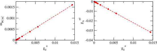
Figure 15: Values for the PCAC quark-mass $m_{\rm PCAC}$ (207) and for $g_{\rm A}^{ud}$, as a function of $g^{4}_{0}$, obtained from Monte Carlo simulations at $L/a=8$. Both quantities have been measured in the middle of the lattice i.e. for $x_{0}=T/2$.

In order to confirm that the bare parameters $m_{0}(g_{0})$ and $z_{f}(g_{0})$ were chosen properly, we checked whether the conditions (75) and (76) were realized up to O($g_{0}^{4}$) corrections. To this end, we looked at the quantities,

$$m_{\rm PCAC}(x_{0})={\tilde{\partial}_{0}g_{\rm A}^{ud}(x_{0})\over 2g_{\rm P}^{ud}(x_{0})}\quad\text{and}\quad g_{\rm A}^{ud}(x_{0}),$$ (207)

which are show in Figure 15. As we can see, the data are very well described by a pure O($g_{0}^{4}$) effect over the whole range of $g_{0}$ we investigated. The renormalization conditions are then satisfied up to 1-loop order in perturbation theory.

Table 4: Comparison between the 1-loop coefficients $Z_{\rm X}^{(1)}(L/a)$ of $Z_{\rm X}$, ${\rm X=V,A}$, for both the $l$ and $g$ definitions, as obtained from perturbation theory (PT) and Monte Carlo simulations (MC) at $L/a=8$.

$Z_{\rm X}^{(1)}(L/a)$	PT	MC
$Z_{\rm V}^{g(1)}$	$-0.122586$	$-0.122596(19)$
$Z_{\rm V}^{l(1)}$	$-0.129838$	$-0.129822(12)$
$Z_{\rm A}^{g(1)}$	$-0.109076$	$-0.109074(22)$
$Z_{\rm A}^{l(1)}$	$-0.116640$	$-0.116645(10)$

In Figure 16, instead, we present the results for the two definitions of $Z_{\rm V}$ (left panel), and $Z_{\rm A}$ (right panel). Specifically, after verifying that $Z_{\rm V}$ and $Z_{\rm A}$ extrapolated correctly to 1 for $g_{0}\to 0$, we looked at $(Z_{\rm X}-1)/g_{0}^{2}$, ${\rm X=V,A}$, in order to extract the 1-loop coefficients $Z_{\rm X}^{(1)}(L/a)$ to be compared with perturbation theory. As we can see from the figure, there is nice agreement between the perturbative and Monte Carlo determinations. We note that $Z_{\rm X}^{(1)}(L/a)$ was obtained from the Monte Carlo data by considering a linear fit of $(Z_{\rm X}-1)/g_{0}^{2}$ with respect to $g_{0}^{2}$, including all but the largest value of $g_{0}$ we simulated. For completeness, we collected in Table 4 the results from 1-loop perturbation theory and the results of the extrapolations of the Monte Carlo data.

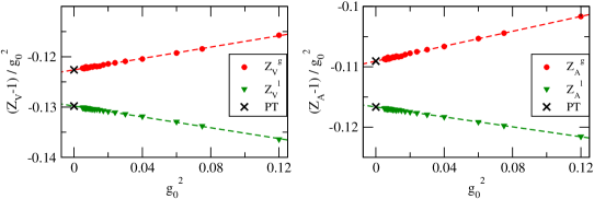
Figure 16: Results for the two definitions of $Z_{\rm V}$, $Z^{g}_{\rm V}$ and $Z^{l}_{\rm V}$, and of $Z_{\rm A}$, $Z^{g}_{\rm A}$ and $Z^{l}_{\rm A}$, as a function of $g^{2}_{0}$, obtained from Monte Carlo simulations at $L/a=8$. The perturbative results, PT, for $Z_{\rm X}^{(1)}(L/a)$, ${\rm X=V,A}$, are also shown.

References

- (1) S. Sint, The Schrödinger functional with chirally rotated boundary conditions, PoS LAT2005 (2006) 235, [hep-lat/0511034].
- (2) S. Sint, The chirally rotated Schrödinger functional with Wilson fermions and automatic O(a) improvement, Nucl. Phys. B847 (2011) 491–531, [arXiv:1008.4857].
- (3) M. Lüscher, R. Narayanan, P. Weisz, and U. Wolff, The Schrödinger functional: a renormalizable probe for non-Abelian gauge theories, Nucl. Phys. B384 (1992) 168–228, [hep-lat/9207009].
- (4) S. Sint, On the Schrödinger functional in QCD, Nucl. Phys. B421 (1994) 135–158, [hep-lat/9312079].
- (5) S. Sint, One loop renormalization of the QCD Schrödinger functional, Nucl. Phys. B451 (1995) 416–444, [hep-lat/9504005].
- (6) S. Miyazaki and Y. Kikukawa, Boundary condition for staggered fermion in lattice Schrödinger functional of QCD, hep-lat/9409011.
- (7) U. M. Heller, The Schrödinger functional running coupling with staggered fermions, Nucl. Phys. B504 (1997) 435–458, [hep-lat/9705012].
- (8) P. Perez Rubio and S. Sint, Fermionic correlation functions from the staggered Schrödinger functional, PoS LATTICE2008 (2008) 221, [arXiv:0810.3866].
- (9) Y. Taniguchi, Schrödinger functional formalism with Ginsparg-Wilson fermion, JHEP 12 (2005) 037, [hep-lat/0412024].
- (10) Y. Taniguchi, Schrödinger functional formalism with domain-wall fermion, JHEP 10 (2006) 027, [hep-lat/0604002].
- (11) S. Sint, Schrödinger functional renormalization schemes for Ginsparg-Wilson quarks, PoS LAT2007 (2007) 253.
- (12) R. Frezzotti and G. C. Rossi, Chirally improving Wilson fermions. 1. O(a) improvement, JHEP 08 (2004) 007, [hep-lat/0306014].
- (13) ALPHA Collaboration, R. Frezzotti, P. A. Grassi, S. Sint, and P. Weisz, Lattice QCD with a chirally twisted mass term, JHEP 08 (2001) 058, [hep-lat/0101001].
- (14) S. Sint and B. Leder, Testing universality and automatic O(a) improvement in massless lattice QCD with Wilson quarks, PoS LATTICE2010 (2010) 265, [arXiv:1012.2500].
- (15) S. Sint and P. Vilaseca, Perturbative lattice artefacts in the SF coupling for technicolor-inspired models, PoS LATTICE2011 (2011) 091, [arXiv:1111.2227].
- (16) S. Sint and P. Vilaseca, Lattice artefacts in the Schrödinger Functional coupling for strongly interacting theories, PoS LATTICE2012 (2012) 031, [arXiv:1211.0411].
- (17) S. Sint and P. Vilaseca, A perturbative study of the chirally rotated Schrödinger Functional in QCD, PoS LATTICE2014 (2014) 279, [arXiv:1412.7928].
- (18) J. Gonzalez Lopez, K. Jansen, D. Renner, and A. Shindler, A quenched study of the Schrödinger functional with chirally rotated boundary conditions: non-perturbative tuning, Nucl. Phys. B867 (2013) 567–608, [arXiv:1208.4591].
- (19) J. Gonzalez Lopez, K. Jansen, D. Renner, and A. Shindler, A quenched study of the Schrödinger functional with chirally rotated boundary conditions: applications, Nucl. Phys. B867 (2013) 609–635, [arXiv:1208.4661].
- (20) M. Dalla Brida and S. Sint, A dynamical study of the chirally rotated Schödinger functional in QCD, PoS LATTICE2014 (2014) 280, [arXiv:1412.8022].
- (21) M. Lüscher, S. Sint, R. Sommer, and P. Weisz, Chiral symmetry and O(a) improvement in lattice QCD, Nucl. Phys. B478 (1996) 365–400, [hep-lat/9605038].
- (22) S. Sint and P. Weisz, Further results on O(a) improved lattice QCD to one-loop order of perturbation theory, Nucl. Phys. B502 (1997) 251–268, [hep-lat/9704001].
- (23) B. Sheikholeslami and R. Wohlert, Improved Continuum Limit Lattice Action for QCD with Wilson Fermions, Nucl. Phys. B259 (1985) 572.
- (24) M. Bochicchio et al., Chiral Symmetry on the Lattice with Wilson Fermions, Nucl. Phys. B262 (1985) 331.
- (25) M. Lüscher, S. Sint, R. Sommer, and H. Wittig, Non-perturbative determination of the axial current normalization constant in O(a) improved lattice QCD, Nucl. Phys. B491 (1997) 344–364, [hep-lat/9611015].
- (26) ALPHA Collaboration, S. Sint and P. Weisz, The running quark mass in the SF scheme and its two-loop anomalous dimension, Nucl. Phys. B545 (1999) 529–542, [hep-lat/9808013].
- (27) ALPHA Collaboration, S. Capitani, M. Lüscher, R. Sommer, and H. Wittig, Non-perturbative quark mass renormalization in quenched lattice QCD, Nucl. Phys. B544 (1999) 669–698, [hep-lat/9810063].
- (28) M. Lüscher and P. Weisz, O(a) improvement of the axial current in lattice QCD to one-loop order of perturbation theory, Nucl. Phys. B479 (1996) 429–458, [hep-lat/9606016].
- (29) P. Weisz, Computation of the improvement coefficient to 1-loop. Unpublished notes (1995).
- (30) S. Sint and R. Sommer, The running coupling from the QCD Schrödinger functional: a one-loop analysis, Nucl. Phys. B465 (1996) 71–98, [hep-lat/9508012].
- (31) ALPHA Collaboration, A. Bode, P. Weisz, and U. Wolff, Two loop computation of the Schrödinger functional in lattice QCD, Nucl. Phys. B576 (2000) 517–539, [hep-lat/9911018].
- (32) A. Gonzalez Arroyo, F. J. Yndurain, and G. Martinelli, Computation of the Relation Between the Quark Masses in Lattice Gauge Theories and on the Continuum, Phys. Lett. B117 (1982) 437. [Erratum: Phys. Lett. B122 (1983) 486].
- (33) J. Stehr and P. H. Weisz, Note on Gauge Fixing in Lattice QCD, Lett. Nuovo Cim. 37 (1983) 173–177.
- (34) R. Wholert, Improved continuum limit lattice action for quarks. DESY preprint 87-069. Unpublished (1987).
- (35) M. Lüscher, R. Sommer, P. Weisz, and U. Wolff, A precise determination of the running coupling in the SU(3) Yang-Mills theory, Nucl. Phys. B413 (1994) 481–502, [hep-lat/9309005].
- (36) A. Hietanen, T. Karavirta, and P. Vilaseca, Schrödinger functional boundary conditions and improvement for , JHEP 11 (2014) 074, [arXiv:1408.7047].
- (37) E. Gabrielli, G. Martinelli, C. Pittori, G. Heatlie, and C. T. Sachrajda, Renormalization of lattice two fermion operators with improved nearest neighbor action, Nucl. Phys. B362 (1991) 475–486.
- (38) G. Martinelli and Y.-C. Zhang, The Connection Between Local Operators on the Lattice and in the Continuum and Its Relation to Meson Decay Constants, Phys. Lett. B123 (1983) 433.
- (39) G. Martinelli and Y.-C. Zhang, One Loop Corrections to Extended Operators on the Lattice, Phys. Lett. B125 (1983) 77.
- (40) B. Meyer and C. Smith, Finite Renormalizations of Currents in Lattice Gauge Theories, Phys. Lett. B123 (1983) 62.
- (41) R. Groot, J. Hoek, and J. Smit, Normalization of Currents in Lattice QCD, Nucl. Phys. B237 (1984) 111–127.
- (42) P. Fritzsch, C. Pena, and D. Preti, Non-perturbative renormalization of tensor bilinears in Schrödinger Functional schemes, PoS LATTICE2015 (2015) 250.
- (43) M. Lüscher, P. Weisz, and U. Wolff, A numerical method to compute the running coupling in asymptotically free theories, Nucl. Phys. B359 (1991) 221–243.
- (44) M. Dalla Brida, M. Papinutto, and P. Vilaseca, Perturbative renormalization of four-fermion operators with the chirally rotated Schrödinger functional, PoS LATTICE2015 (2015) 252.
- (45) M. Dalla Brida, T. Korzec, M. Papinutto, and P. Vilaseca, The chirally rotated Schrödinger functional at work, talk given at: The 33rd International Symposium on Lattice Field Theory (Lattice 2015), 14–18 July 2015, Kobe, Japan.
- (46) M. Dalla Brida, S. Sint, and P. Vilaseca, Non-perturbative tests of universality and automatic O() improvement in two-flavour QCD, in preparation.
- (47) M. Dalla Brida, T. Korzec, S. Sint, and P. Vilaseca, High precision renormalization of the non-singlet axial current in lattice QCD with Wilson quarks, in preparation.
- (48) S. Sint and P. Weisz, Further one-loop results in O(a) improved lattice QCD, Nucl. Phys. Proc. Suppl. 63 (1998) 856–858, [hep-lat/9709096].