Model-Based Iterative Reconstruction
for Radial Fast Spin-Echo MRI

Abstract

In radial fast spin-echo MRI, a set of overlapping spokes with an inconsistent T2 weighting is acquired, which results in an averaged image contrast when employing conventional image reconstruction techniques. This work demonstrates that the problem may be overcome with the use of a dedicated reconstruction method that further allows for T2 quantification by extracting the embedded relaxation information. Thus, the proposed reconstruction method directly yields a spin-density and relaxivity map from only a single radial data set. The method is based on an inverse formulation of the problem and involves a modeling of the received MRI signal. Because the solution is found by numerical optimization, the approach exploits all data acquired. Further, it handles multi-coil data and optionally allows for the incorporation of additional prior knowledge. Simulations and experimental results for a phantom and human brain in vivo demonstrate that the method yields spin-density and relaxivity maps that are neither affected by the typical artifacts from TE mixing, nor by streaking artifacts from the incomplete k-space coverage at individual echo times.

Keywords. turbo spin-echo, radial sampling, non-Cartesian MRI, iterative reconstruction, inverse problems.

Copyright 2009 IEEE. Personal use of this material is permitted. Permission from IEEE must be obtained for all other uses, in any current or future media, including reprinting/republishing this material for advertising or promotional purposes, creating new collective works, for resale or redistribution to servers or lists, or reuse of any copyrighted component of this work in other works. Published in final form in:
IEEE Transactions on Medical Imaging 28:1759-1769 (2009)
DOI: 10.1109/TMI.2009.2023119

1 Introduction

Fast spin-echo (FSE) MRI is one of the most frequently used MRI techniques in today’s clinical practice. In the FSE technique, a train of multiple spin-echoes is generated after each RF excitation. Therefore, it offers images with proton-density (PD) and T2 contrast at a significantly reduced measuring time compared to a spin-echo sequence with a single phase-encoding step per excitation. Although the k-space lines that are sampled during each train of spin echoes have different echo times (TE) and, thus, increasing T2 weighting, conventional Cartesian sampling strategies still allow for a straightforward image reconstruction with only minor artifacts under visual inspection when grouping spin echoes with equal echo time around the center of k-space. The underlying reason is the dominance of major image features by the centrally located low spatial frequencies, while the periphery of k-space rather defines edges which are less susceptible to changes in the contrast weighting. Moreover, in the Cartesian case, the contrast of the image can be adjusted by reordering the acquisition scheme such that the central k-space lines are measured with the desired echo time. A noticeable disadvantage of the T2 attenuation in k-space, however, is a certain degree of image blurring. It arises because the signal decay can be formally written as a multiplication of the true k-space data with some envelope function, which yields a convolution in image space along the phase encoding direction.

In recent years, radial sampling, as originally proposed by Lauterbur [1], has regained considerable interest as an alternative to Cartesian sampling. In this technique, coverage of k-space is accomplished by sampling the data along coinciding spokes instead of parallel lines. Radial sampling offers several promising advantages that include a lower sensitivity to object motion [2, 3], the absence of any ghosting effects, and efficient undersampling properties. In principle, radial trajectories can be combined with almost all MRI techniques including FSE sequences [2, 3, 4]. In this specific case, however, the modified sampling scheme has major implications for the image reconstruction procedure. Because all spokes pass through the center of k-space, each spoke carries an equal amount of low spatial frequency information which, for different echo times, exhibits pronounced differences in T2 contrast. This situation is fundamentally different to the Cartesian case and poses complications when employing conventional reconstruction methods such as filtered backprojection or gridding [5]: (i) The merging of spokes with different echo times may cause streaking artifacts around areas with pronounced T2 relaxation because the relative signal decay leads to jumps in the corresponding point-spread-function [6]. (ii) The contrast of the image always represents an average of the varying T2 weightings. (iii) Differently ordered k-space acquisitions may no longer be used to alternate the image contrast and, thus, to distinguish between PD and T2 relaxation. On the other hand, because all spokes pass through the center of k-space and capture the low spatial frequencies at every echo time, a single radial FSE data set implicitly contains information about the local signal decay. Therefore, dedicated reconstruction methods have been developed that extract this embedded temporal information in order to quantify the T2 relaxation within a reduced measurement time relative to Cartesian-based T2 quantification approaches.

Most of the existing techniques, such as k-space weighted image contrast (KWIC) [7, 8], attempt to calculate a series of echo time-resolved images by mixing the low spatial frequencies from spokes measured at the desired echo time with high frequency information from other spokes (measured at different echo times). A drawback of these techniques is that the TE mixing tends to cause artifacts in the reconstructed images. Although their strength can be attenuated to some degree with specific echo mixing schemes [8], these artifacts limit the accuracy of the T2 estimates. In particular, the values become dependent on the object size as the change in k-space is assumed to be located only in the very central area that is densely covered by spokes measured at an equal echo time [8].

To overcome the limitation, this work demonstrates an iterative concept for the reconstruction from radially sampled FSE acquisitions. Instead of calculating any intermediate images, the proposed method estimates a spin density and a relaxivity map directly from the acquired k-space data using a numerical optimization technique. Because the procedure involves a modeling of the received MRI signal that accounts for the time dependency of the acquired samples, the approach exploits the entire data for finding these maps without assuming that the contrast changes are restricted to a very central area of k-space. Related ideas have been presented by Graff et al [9] and Olafsson et al [10].

2 Theory

The method proposed here can be seen as an extension of a previous development for the reconstruction from highly undersampled radial acquisitions with multiple receive coils [11]. In this work, the reconstruction is achieved by iteratively estimating an image that, on the one hand, is consistent with the measured data and, on the other hand, complies with prior object knowledge to compensate for the missing data. For multi-echo data from a FSE sequence, this strategy is not appropriate because it is impossible to find a single image that matches the different contrasts at the same time. Therefore, it is necessary to include the relaxation process into the signal modeling used to compare the image estimate to the measured k-space samples. As the T2 relaxation time is a locally varying quantity, this requires that the estimate consists of a spin-density and a relaxation component instead of just an intensity component, which directly yields a quantification of the relaxation time. The objective of the present extended approach, therefore, is to simultaneously find a spin-density map and a relaxivity map such that snapshots, calculated for each echo time from these maps, best match the spokes measured at the respective echo times.

2.1 Cost Function

In order to compute the maps, a cost function is needed which quantifies the accuracy or quality of the match to the measured data, such that the optimal solution can be identified by a minimum value of this function. Because experimental MRI data is always contaminated by a certain degree of Gaussian noise, the cost function of the proposed method uses the L2 norm and has the form

$$\Phi(\vec{\rho},\vec{r})=\frac{1}{2}\sum_{t}\sum_{c}\left\|\vec{F}(\vec{\rho},\vec{r},t,c)-\vec{y}_{t,c}\right\|^{2}_{2}\;,$$ (1)

where $\vec{\rho}$ is a vector containing the values of the spin-density map, and $\vec{r}$ is a vector containing values of the relaxivity map. For a base resolution of $n\times n$ pixels, both vectors have $n^{2}$ entries. Further, $\vec{y}_{t,c}$ is a vector containing the raw data from channel $c$ of all spokes measured at echo time $t$, where $c$ runs from 1 to the total number of receive channels and $t$ runs over all echo times. Finally, $\vec{F}$ is a vector function that calculates a snapshot from the given spin-density and relaxivity map at echo time $t$, and translates it to k-space using a Fourier transformation and subsequent evaluation at the sampling positions of the spokes acquired at time $t$. Moreover, before Fourier transformation, the mapping includes a multiplication with the sensitivity profile of coil $c$. These coil profiles are estimated from the same data set in a preceding processing step using a sum-of-squares combination of the channels, where it is assumed that the individual sensitivity profiles are smooth functions. A detailed description of this procedure is given in [11].

The function $\vec{F}$ can be seen as the forward operation of the reconstruction problem and comprises a model of the received MRI signal, which is used to synthesize the corresponding k-space signal from the given maps. The $j$th entry, i.e. the $j$th sample of the synthesized data with k-space position $\vec{k}_{j}$ at echo time $t$, is given by

$$F_{j}(\vec{\rho},\vec{r},t,c)=\sum_{\vec{x}\in\textrm{FOV}}\varrho(\vec{x})\cdot e^{-R(\vec{x})\cdot t}\cdot C_{c}(\vec{x})\cdot e^{-i\,\vec{x}\cdot\vec{k}_{j}}\,,$$ (2)

where $\vec{x}$ denotes a position in image space such that the sum runs over all (discrete) elements of the image matrix, and $C_{c}$ is the complex sensitivity profile of the $c$th coil. Further, $\varrho$ denotes a function which evaluates the spin-density vector $\vec{\rho}$ at image position $\vec{x}$

$$\varrho(\vec{x})=\sum_{i}\rho_{i}\cdot\delta(\vec{x}-\vec{x_{i}})\;,$$ (3)

where $\rho_{i}$ denotes the $i$th component of the spin-density vector with corresponding position $\vec{x_{i}}$ in image space. Accordingly, the function $R$ evaluates the relaxivity vector $\vec{r}$

$$R(\vec{x})=\sum_{i}r_{i}\cdot\delta(\vec{x}-\vec{x_{i}})\;.$$ (4)

To reconstruct a set of measured data $\vec{y}$, a pair of vectors $(\vec{\rho},\vec{r})$ has to be found that minimizes the cost function $\Phi$. This can be achieved by using a numerical optimization method that is suited for large-scale problems, like the non-linear conjugate-gradient (CG) method. Here, we employed the CG-Descent algorithm recently presented by Hager and Zhang [12], which can be used in a black box manner. Hence, it is only required to evaluate $\Phi$ and its gradient at given positions $(\vec{\rho},\vec{r})$ in the parameter space.

2.2 Evaluation of Cost Function

Evaluation of the cost function at a given pair $(\vec{\rho},\vec{r})$ can be done in a straightforward manner. However, to calculate the value of $\Phi$ in a reasonable time, a practical strategy is to perform a fast Fourier transformation (FFT) of the snapshots and to interpolate the transforms onto the desired spoke positions in k-space using a convolution with a radial Kaiser-Bessel kernel similar to the gridding technique [5, 13]. Because the kernel is finite, it is further necessary to pre-compensate for undesired intensity modulations by multiplying the snapshots with an approximation of the kernel’s Fourier transform in front of the FFT – commonly known as roll-off correction [14].

The same strategy can be used for evaluating the gradient, which is a vector containing the derivative of the cost function with respect to each component of the spin-density and relaxivity vector. It is convenient to decompose the problem into a separate derivation of $\Phi$ with respect to components of $\vec{\rho}$ and $\vec{r}$, respectively,

$$\nabla\Phi=\left(\begin{array}[]{c}\nabla_{\rho}\Phi\\ \nabla_{r}\Phi\end{array}\right)\;.$$ (5)

To simplify the notation, the calculation is only shown for a single time point and a single coil (indicated by $\phi$ instead of $\Phi$)

$$\phi=\frac{1}{2}\left\|\vec{F}-\vec{y}\right\|^{2}_{2}\;.$$ (6)

Derivation of Eq. (2) with respect to components of $\vec{\rho}$ gives

$$\frac{\partial F_{j}}{\partial\rho_{v}}=e^{-R(\vec{x}_{v})\cdot t}\cdot C_{c}(\vec{x}_{v})\cdot e^{-i\,\vec{x}_{v}\cdot\vec{k}_{j}}\;,$$ (7)

where $\vec{x}_{v}$ denotes the position of the $v$th component in image space. Using the chain rule and inserting this equation then yields (see Appendix)

$$\frac{\partial}{\partial\rho_{v}}\phi=e^{-R(\vec{x}_{v})\cdot t}\cdot\Re\left\{\overline{C_{c}(\vec{x}_{v})}\cdot\sum_{j}\left(F_{j}-y_{j}\right)e^{i\,\vec{x}_{v}\cdot\vec{k}_{j}}\right\}.$$ (8)

Hence, the gradient with respect to $\vec{\rho}$ can be obtained by evaluating the cost function, calculating the residual, and performing an inverse Fourier transformation, which is followed by a multiplication with the complex conjugate of the coil profile and, finally, with the relaxation term. Derivation of Eq. (2) with respect to components of $\vec{r}$ gives

$$\frac{\partial F_{j}}{\partial r_{v}}=-t\cdot\varrho(\vec{x}_{v})\cdot e^{-R(\vec{x}_{v})\cdot t}\cdot C_{c}(\vec{x}_{v})\cdot e^{-i\,\vec{x}_{v}\cdot\vec{k}_{j}}$$ (9)

and, in a similar way to (8), this yields

$$\frac{\partial}{\partial r_{v}}\phi = -t\cdot\varrho(\vec{x}_{v})\cdot e^{-R(\vec{x}_{v})\cdot t}\cdot\Re\left\{\overline{C_{c}(\vec{x}_{v})}\cdot\sum_{j}\left(F_{j}-y_{j}\right)e^{i\,\vec{x}_{v}\cdot\vec{k}_{j}}\right\}.$$ (10)

Comparison with Eq. (8) shows that the gradient with respect to $\vec{r}$ can be easily obtained by multiplying the gradient with respect to $\vec{\rho}$ with the components of the given $\vec{\rho}$ and the echo time $t$. Of course, Eq. (8) and Eq. (10) have to be summed over each channel and echo time occurring in the complete cost function (1).

2.3 Regularization

Because the aforementioned strategy for fast evaluation of the cost function involves an interpolation step that is imperfect in practice, and, further, because the measured values correspond to the continuous Fourier transform whereas the estimated maps are discrete, it is necessary to introduce a regularization of the estimate. If a regularization is not used, implausible values arise after a certain number of iterations in ill-conditioned areas of the estimate, i.e. in entries of the maps that are not well-defined from the measured k-space values. For instance, the edges of the maps’ Fourier transforms outside of the sampled disc are ill-conditioned due to a lack of measured samples in these areas. Because the optimizer simply tries to reduce the total value of the cost function, it employs such “degrees of freedom” to minimize the residuum at neighboring sampling positions (it should be noted that the interpolation strategy assumes that the true function can be locally approximated by a weighted sum over the nearby grid points). This results in local k-space peaks with high amplitude that translate into noise-alike image patterns for high iteration numbers. The problem poses a general drawback of the iterative reconstruction technique, which can be either adressed by stopping the optimization procedure after some iterations or by regularizing the estimate to suppress implausible values. Advantages of the latter approach are that the estimate converges to a well-defined solution without being sensitive to the total iteration number and that it allows for tuning the solution by using different regularization techniques. A regularization is accomplished by complementing the cost function with a weighted penalty function $P(\vec{\rho},\vec{r})$ which can act on both the spin-density and relaxivity map

$$\Phi(\vec{\rho},\vec{r}) = \frac{1}{2}\sum_{t}\sum_{c}\left\|\vec{F}(\vec{\rho},\vec{r},t,c)-\vec{y}_{t,c}\right\|^{2}_{2}+\lambda\cdot P(\vec{\rho},\vec{r})\;.$$ (11)

Different types of penalty functions can be used for the regularization. For instance, constraining the total energy of the estimate by penalizing the L2 norm of its components leads to the commonly known (simple) Tikhonov regularization. In the present work, the L2 norms of the finite differences of the maps’ Fourier transforms are penalized, which enforces certain smoothness of the k-space information

$$P(\vec{\rho},\vec{r})=\left\|D_{x}\mathcal{F}\,\vec{\rho}\right\|^{2}_{2}+\left\|D_{y}\mathcal{F}\,\vec{\rho}\right\|^{2}_{2}+\left\|D_{x}\mathcal{F}\,\vec{r}\right\|^{2}_{2}+\left\|D_{y}\mathcal{F}\,\vec{r}\right\|^{2}_{2}\;.$$ (12)

Here, $\mathcal{F}$ denotes the discrete Fourier transformation, and $D_{x}$ is the finite difference operator in x-direction

$$D_{x}\,\textrm{I}(x,y)=\textrm{I}(x,y)-\textrm{I}(x-1,y)\;.$$ (13)

It turned out that this choice offers robust suppression of local intensity accumulations in the ill-conditioned areas, so that no artifacts appear even for a high number of iterations (e.g., 1000 iterations).

A drawback of any regularization technique is that it introduces a weighting factor $\lambda$, which has to be chosen properly. If selected too low, the regulariation becomes ineffective, whereas if selected too high, the solution will be biased towards the minimization of the penalty term (here leading to an undesired image modulation). A method for automatically determining the proper regularization weight would be highly desirable, but the establishment of such a method is yet an open issue. However, with the penalty term described in Eq. (12), the reconstruction appears to be rather insensible to minor changes of the weighting factor $\lambda$. In fact, all images presented here were obtained with a fixed value of $\lambda=0.001$, which yielded an effective artifact suppression without noticeably affecting the results. Presumably, the weight has to be adjusted for measured data with completely different scaling. In this case, a reasonable adjustment strategy is to start with a very small weight and to increase the value successively until the artifacts visually disappear.

2.4 Initialization

In the single-echo reconstruction scenario, it is very efficient to initialize the optimizer with a properly scaled gridding solution. This choice significantly reduces the total number of iterations because the optimizer starts with a reasonable guess. In the multi-echo case, however, it is more difficult to obtain reasonable initial guesses for the spin-density and relaxivity map, and several options exist. For example, a curve fitting of either strongly undersampled or low-resolution gridding solutions from single echo times could be used to approximate the maps. Alternatively, an echo-sharing method like KWIC could be employed. While preliminary analyses confirmed that these strategies may lead to a certain acceleration of convergence, they also indicated complications if the initial guesses contain implausible values, for example, in relaxation maps which are obviously undefined in areas with a void signal intensity. It is therefore necessary to remove respective values from the initial guesses. The present work simply used zero maps for the initialization, which require a higher number of iterations but ensure a straightforward convergence to a reasonable solution.

2.5 Scaling and Snapshot Calculation

Another factor with essential impact on the convergence rate is the scaling of the time variable $t$. Although it intuitively makes sense to directly use physical units, a proper rescaling of the time variable significantly reduces the number of iterations. Equation (10) shows that the gradient with respect to the relaxivity depends linearly on $t$, while this is not the case with respect to the spin density. If the values of $t$ for the different echoes are very small, then the cost function is much more sensitive to changes in $\vec{\rho}$ and the problem is said to be poorly scaled [15]. In contrast, large values of $t$ lead to a dominant sensitivity to perturbations in $\vec{r}$. Because finding a reasonable solution requires a matching of both maps at the same time, the optimization procedure is especially effective when the scaling of $t$ is selected such that there is a balanced influence on the cost function. In our experience, a proper scaling, which depends on the range of the object’s spin-density and relaxivity values, allows for reducing the number of required iterations from over 1000 iterations to about only 80 iterations for a typical data set. Of course, a rescaling of $t$ is accompanied by a corresponding scaling of the relaxivity values in $\vec{r}$, which can be corrected afterwards to allow for quantitative analyses. Noteworthy, the sensitivity to scaling is a property of the specific optimization method used here (the non-linear CG method) and not related to the reconstruction concept itself. Hence, exchanging the CG method by an optimization technique that is scale invariant (like the Newton’s method) might render a rescaling unnecessary but is accompanied by other disadvantages like calculation of the Hessian [15].

Finally, after complete estimation of the spin-density map $\vec{\rho}$ and relaxivity map $\vec{r}$, snapshot images can be calculated for an arbitrary echo time with

$$I_{t}(\vec{x})=\varrho(\vec{x})\cdot e^{-R(\vec{x})\cdot t}\;.$$ (14)

These images do not contain any additional information, but present the estimated temporal information in a more familiar view.

3 Methods

3.1 Data Acquisition

For evaluation of the proposed reconstruction technique, simulated data and experimental MRI data was used. The simulated data was created with a numerical phantom which is composed of superimposed ellipses so that the analytical Fourier transform of the phantom can be deduced from the well-known Fourier transform of a circle. The numerical phantom mimics a water phantom consisting of three compartments with different T2 relaxation times (200 ms, 100 ms, and 50 ms), which are surrounded by a compartment with a relaxation time comparable to that of pure water (1000 ms). All experiments were conducted at 2.9 T (Siemens Magnetom TIM Trio, Erlangen, Germany) using a receive only 12-channel head coil in circularly polarized (CP) mode, yielding four channels with different combinations of the coils. Measurements were performed for a water phantom doped with $\textrm{MnCl}_{2}$ as well as the human brain in vivo, where written informed consent was obtained in all cases prior to each examination.

The simulated data and the experimental phantom data was acquired with a base resolution of 160 pixels covering a FOV of 120 mm (bandwidth 568 Hz/pixel), while human brain data was acquired with a base resolution of 224 pixels covering a FOV of 208 mm (bandwidth 360 Hz/pixel). A train of 16 spin echoes with an echo spacing of 10 ms was recorded after a slice-selective 90^∘ excitation pulse (section thickness 3 mm). The spin echoes were refocused using a conventional 180^∘ RF pulse, enclosed by crusher gradients to dephase spurious FID signals. The total number of spokes per data set ranged from 128 to 512 spokes, which were acquired using 8 to 32 excitations and measured with a repetition time of TR = 7000 ms to avoid saturation effects of the CSF. The ”angular bisection” view-ordering scheme was used as described by Song and Dougherty [7], which ensures that spokes measured at consecutive echo times have a maximum angular distance. Noteworthy, this scheme is not required by the proposed method, but it was employed to permit reconstructions with the KWIC approach for comparison. Further, the sampling direction of every second repetition was altered in such a way as to generate opposing neighboring spokes. The procedure yields more tolerable artifacts in the presence of off-resonances. Fat suppression was accomplished by a preceding CHESS pulse, and an isotropic compensation mechanism was applied to avoid gradient timing errors and corresponding smearing artifacts due to misalignment of the data in k-space [16]. For comparison, a fully-sampled Cartesian data set of the human brain was acquired with a multi-echo spin-echo sequence from the manufacturer (base resolution 192 pixels, section thickness 4 mm, 16 echoes, echo spacing 10ms, TR = 7000 ms). In this case, k-space was fully sampled at all 16 echo times so that the acquisition time was about 22.4 minutes for a single slice. Moreover, simulations with different degrees of undersampling as well as simulations with added Gaussian noise were performed for appraising the achievable reconstruction accuracy.

3.2 Reconstruction

All data processing was done offline using an in-house software package written in C/C++. In a first step, phase offsets were removed by aligning the phase of all spokes at the center of k-space. Coil sensitivity profiles were estimated from the data set using the procedure described in [11]. In addition, a thresholding mask was obtained from the smoothed sum-of-squares image, so that areas with void signal intensity could be set to zero by applying the mask to all reconstructed images. For the interpolation in k-space from grid to spokes and vice versa, a Kaiser-Bessel window with $L=6$, $\beta=13.8551$ and twofold oversampling was used [17]. To speed up the iterations, the interpolation coefficients were precalculated and stored in a look-up table. The optimizer for estimating the spin-density and relaxivity map was run for a fixed number of 200 iterations to ensure that the estimate has converged, although fewer iterations are usually sufficient for finding an accurate solution. Hence, an automatic stopping criterion would be highly desirable for routine use to avoid unnecessary computation time. The scaling of the time variable was chosen heuristically such that $t=300\cdot n$ for the phantom study and $t=150\cdot n$ for human brain data, where $n$ is the echo number. Because this factor is object-dependent and has significant impact on the optimization efficiency, it would be highly desirable to employ an automatic mechanism for adjusting the scaling. Such development, however, is outside the scope of this work.

For comparison, gridding reconstructions of the spokes measured at each echo time were calculated using the same interpolation kernel. Here, the estimated coil sensitivity profiles were used to combine the different channels instead of taking a sum-of-squares. Further, time-resolved reconstructions employing the KWIC method were calculated. In the initial KWIC work [7], only 8 instead of 16 echoes were acquired per excitation. Therefore, we implemented two variants: either high frequency information from all spokes was used to fill the outer k-space area (kwic 16), or (in a sliding window manner) information from only the 8 neighboring echo times was shared (kwic 8). Apart form that, our implementation followed the basic KWIC approach described in [7]. To allow for a fair comparison, the same interpolation kernel was used, and coil profiles were employed for channel combination. Finally, spin-density and relaxivity maps were estimated from the images by a pixelwise curve fitting using the Levenberg-Marquardt algorithm.

4 Results

4.1 Experimental Data

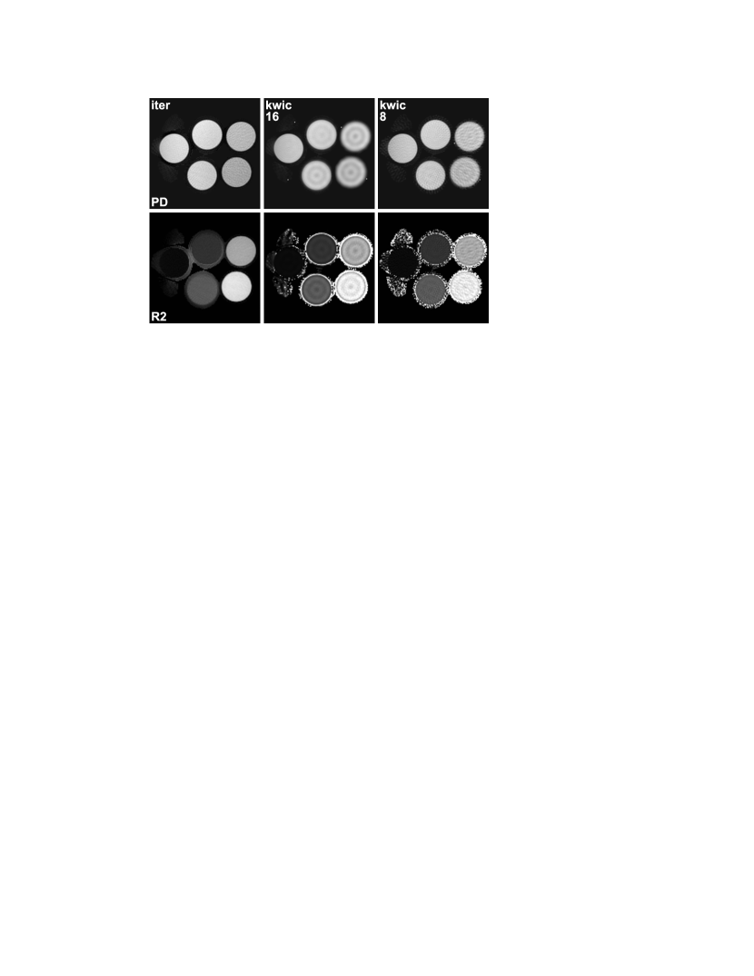
Figure 1: Spin-density maps (top) and relaxivity maps (bottom) estimated for a phantom data set (base resolution 160 pixels, FOV 120 mm, bandwidth 568 Hz/pixel bandwidth) using the proposed iterative method (iter), KWIC combining all 16 echoes (kwic 16), and KWIC combining only 8 neighboring echoes (kwic 8). The images were acquired with a radial FSE sequence using 32 repetitions and 16 echoes each, yielding a total of 512 spokes. PD = proton density, R2 = T2 relaxivity.

Figure  1 compares spin-density and relaxivity maps for a phantom containing five water-filled tubes with different concentrations of $\textrm{MnCl}_{2}$, i.e. different T2 relaxation times, which were estimated using the proposed method, the KWIC method sharing all echoes, and the KWIC method sharing 8 neighboring echoes. It can be seen that the sharing of k-space data in the KWIC reconstructions leads to ring-like artifacts inside the tubes with fast T2 relaxation, in line with the findings of Altbach et al [8]. The artifacts are more pronounced in the KWIC variant sharing all echoes, while the variant sharing only 8 echoes suffers from streaking artifacts due to incomplete coverage of the outer k-space. Such artifacts do not appear in the iteratively estimated maps. Here, the spin-density of the tube with the shortest relaxation time is slightly underestimated, which is probably caused by a higher amount of noise due to fast signal decay. Further, because the relaxivity is undefined in areas with a void spin density, the relaxivity maps are affected by spurious values outside of the tubes in all cases. It should be noted that this effect is limited to a narrow surrounding of the object due to the application of a thresholding mask. In general, these spurious values are distinguishable from the object by a lack of intensity in either the spin-density map or the gridding image from all spokes.

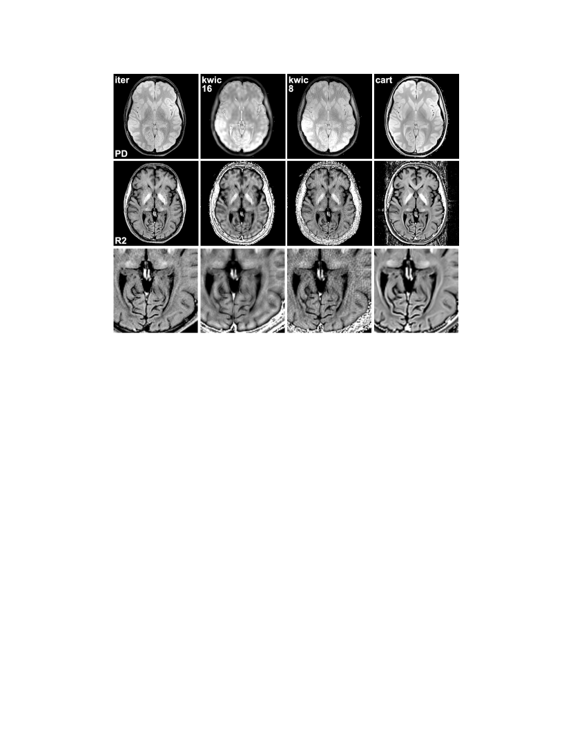
Figure 2: Spin-density maps (top) and relaxivity maps (bottom) estimated for a transverse section of the human brain in vivo (base resolution 224 pixels, FOV 208 mm, bandwidth 360 Hz/pixel) using the proposed method (iter), KWIC combining all 16 echoes (kwic 16), and KWIC combining only 8 neighboring echoes (kwic 8). Other parameters as in Fig. 1. For comparison, maps from a fully-sampled Cartesian reference data set are shown in the right column (cart). The bottom row shows magnifications of the relaxivity maps.

Figure 2 shows corresponding reconstructions for a transverse section of the human brain in vivo. Again, the KWIC reconstruction using 8 echoes suffers from streaking artifacts, while the maps involving all echoes appear fuzzy and blurry. In the latter case, the spin-density map is further contaminated by sharp hyperintense structures. This results from padding the high frequencies with data from late echoes which introduces components with T2 weighting and poses a general problem when sharing data with varying contrast. The iteratively calculated maps present without these artifacts. For comparison, maps from a fully-sampled Cartesian data set are presented, which show good agreement with the maps obtained from the iterative approach. Noteworthy, because the slice thickness was higher in the Cartesian acquisition, these maps show a slightly larger part of the frontal ventricles, which, however, is not related to the reconstruction technique.

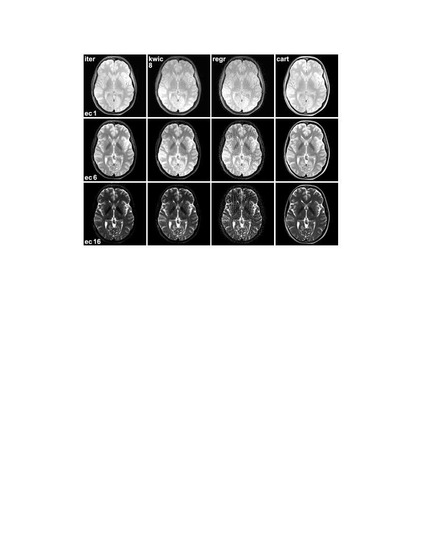
Figure 3: Snapshot reconstructions of the human brain (same data as Fig. 2) at the time of the first (ec1), 6th (ec6), and last echo (ec16) using the proposed method (iter), KWIC combining 8 neighboring echoes (kwic 8), and direct gridding of the single echoes (regr). The right column shows images from a fully-sampled Cartesian data set (cart).

For the same radial data set, Fig. 3 compares snapshots of the first, 6th, and last echo reconstructed using the proposed method with Eq. (14), direct gridding, and KWIC with sharing of 8 echoes. Corresponding images from the Cartesian data set are shown as reference. The contrast of the Cartesian and gridding images can be taken as ground truth due to the equal echo time of all k-space data used. It can be seen that the snapshots calculated with the proposed method show good match to the contrast of the Cartesian gold standard while they are not affected by streaking artifacts.

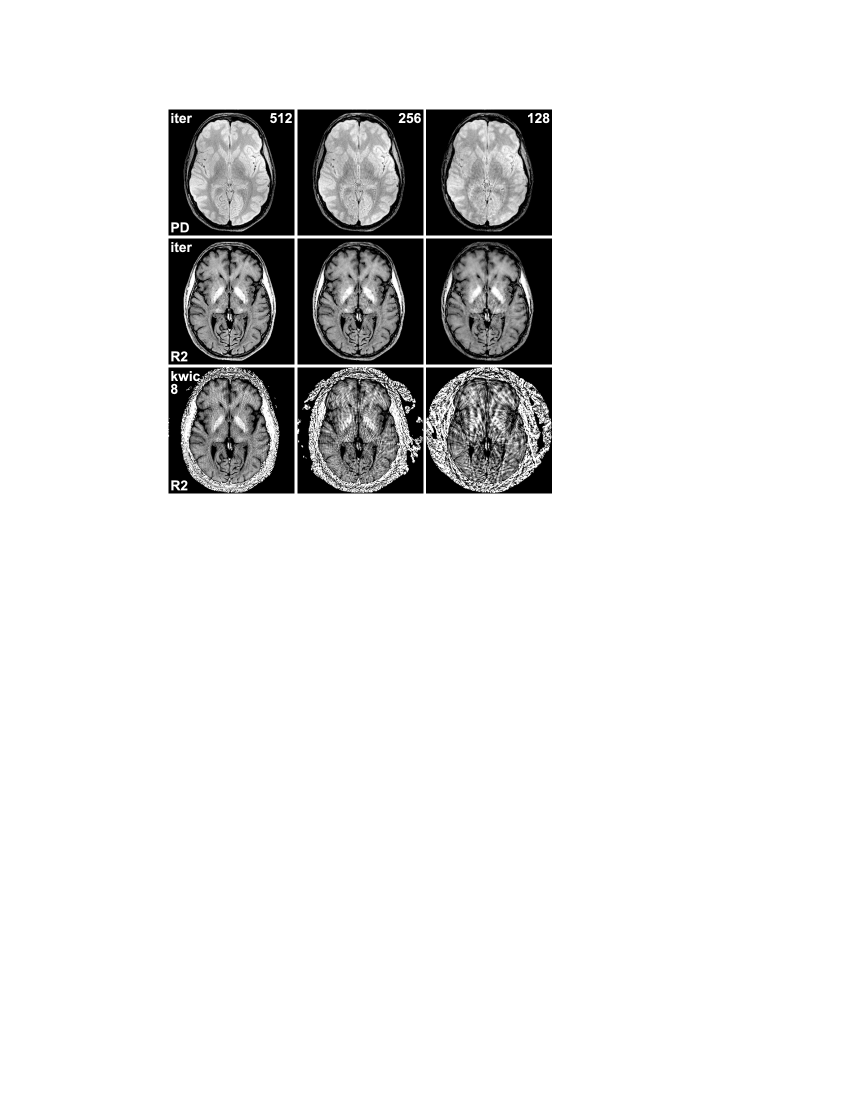
Figure 4: Spin-density maps (PD) and relaxivity maps (R2) estimated using the iterative approach for a transverse section of the human brain in vivo from (left) 512 spokes acquired with 32 repetitions, (middle) 256 spokes acquired with 16 repetitions, and (right) 128 spokes acquired with 8 repetitions (16 echoes each, base resolution 224 pixels, FOV 208 mm, bandwidth 360 Hz/pixel). The bottom row shows relaxivity maps obtained from the same data using the KWIC approach (kwic8).

Finally, Fig. 4 shows iterative reconstructions of the human brain from radial data with different degrees of undersampling, ranging from a total of 512 spokes (32 repetitions) to only 128 spokes (8 repetitions). As expected, the data reduction is accompanied by some loss of image quality, but even for 128 spokes the iterative approach still offers a relatively good separation of proton density and relaxivity. For comparison, relaxivity maps obtained by the KWIC approach are shown in the bottom row, and it can be seen that the image quality breaks down for higher degrees of undersampling.

4.2 Simulated Data

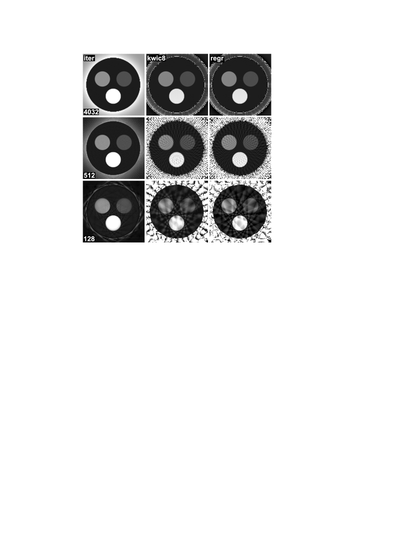
Figure 5: Relaxivity maps estimated from simulated data with (top) 4032 spokes from 252 repetitions (all echoes fully sampled), (middle) 512 spokes from 32 repetitions, and (bottom) 128 spokes from 8 repetitions using (iter) the proposed iterative approach, (kwic8) the KWIC approach sharing 8 neigboring echoes, and (regr) direct gridding of the single echoes (16 echoes each, base resolution 160 pixels). The numerical phantom consists of compartments with relaxations times of T2=200 ms, T2=100 ms, and T2=50 ms which are surrounded by a compartment with T2=1000 ms.

Figure 5 shows relaxivity maps from simulated data estimated with the proposed method, the KWIC method, and direct gridding (the proton density maps are not shown as the proton density was set to a constant value within the phantom). As in the prior figures, an identical windowing function has been used for all relaxivity maps within the figure, so that absolute relaxivity values were equally mapped to grayscale values. The upper row corresponds to a fully sampled data set (4032 spokes, 252 repetitions), and, hence, the number of spokes for each echo time complies with the Nyquist theorem in the sense that the angular distance between neighboring spokes is less or equal to $\Delta k=1/\textrm{FOV}$. In this case, all three approaches yield maps without any streaking artifacts. However, the maps created by KWIC and gridding present with somewhat stronger Gibbs ringing artifacts, which are especially visible within the smaller compartments. The middle row corresponds to the degree of undersampling that was used in the experiments presented in Fig. 1 – Fig. 3 (512 spokes, 32 repetitions). Here, streaking artifacts appear for KWIC and gridding, whereas the iterative reconstruction is free from these artifacts. The bottom row shows maps for a high degree of undersampling, corresponding to the highest undersampling factor presented in Fig. 4 (128 spokes, 8 repetitions). For such an undersampling, minor streaking artifacts arise also in the iterative reconstruction, while the KWIC and gridding reconstructions exhibit severe streaking artifacts. Noteworthy, only a single receive channel was generated in the simulations, and, thus, it clarifies that the proposed method offers an improvement also without exploiting localized coil sensitivities, which is implicitly done for experimental multi-coil data due to the better conditioning of the problem. Table 2 summarizes a region-of-interest (ROI) analysis of the relaxivity maps from Fig. 5, where identical regions were analyzed in all maps. In all cases, the iterative approach estimates the signal relaxivity with higher accuracy than gridding or KWIC. Interestingly, even in the fully-sampled case, significant deviations occur for the KWIC and gridding reconstruction. These deviations result from the strong ringing effects that are apperent in Fig. 5, which appear to be more pronounced for radial acquisitions than for Cartesian acquisitions. Hence, the strong signal from the surrounding compartment smears into the quickly decaying compartments, which causes a bias of the signal intensity in the time-resolved images. The iterative approach seems to better cope with this situation.

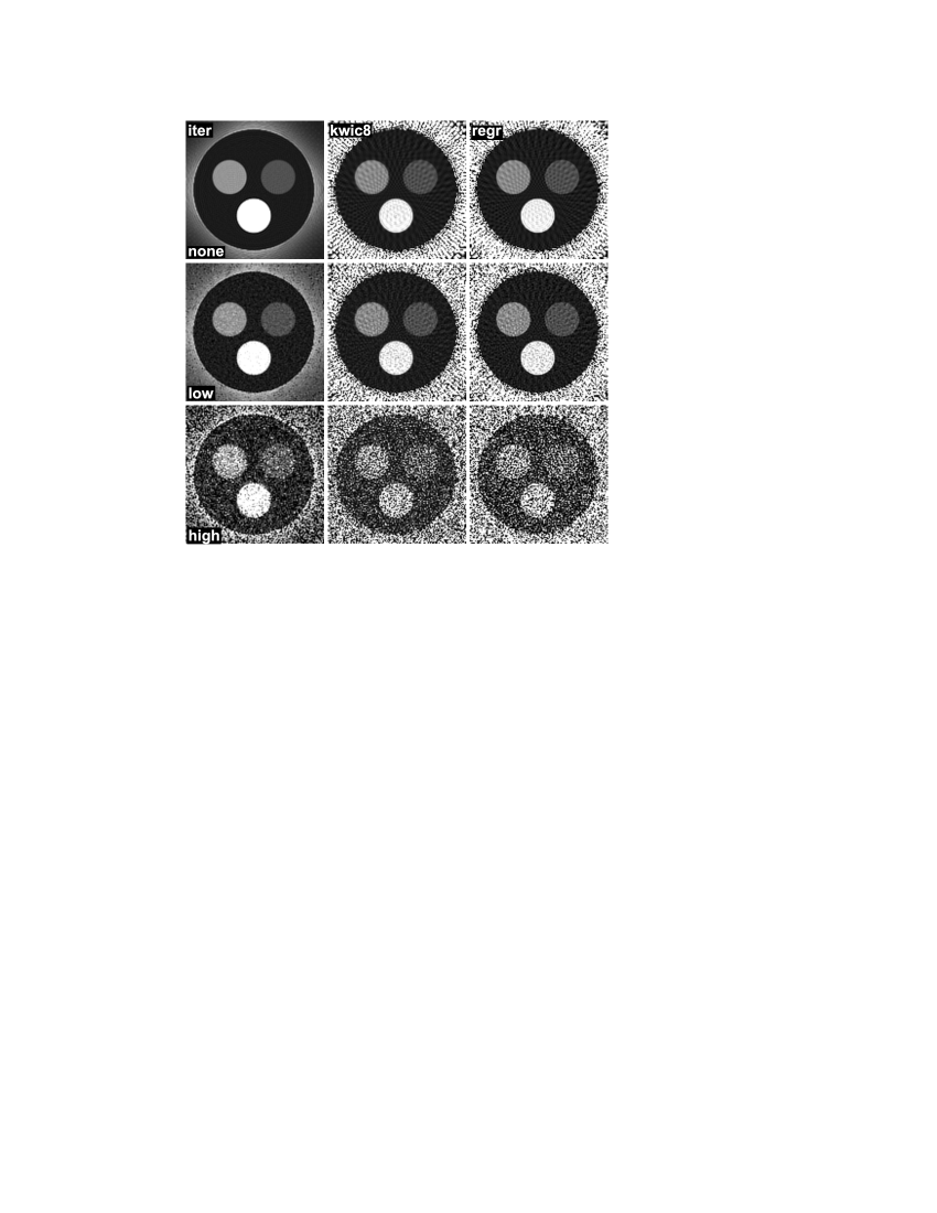
Figure 6: Relaxivity maps estimated from simulated data (top) without noise, (middle) with a low level of Gaussian noise, and (bottom) with a high level of Gaussian noise using (iter) the proposed iterative approach, (kwic8) the KWIC approach sharing 8 neigboring echoes, and (regr) direct gridding of the single echoes (512 spokes from 32 repetitions, 16 echoes each, base resolution 160 pixels). Relaxation times of the numerical phantom as in Fig. 5.

Noise level True T2 Iterative KWIC8 Gridding none Compartment 1 50 ms $50.2\pm 0.1$ ms $60.1\pm 0.3$ ms $59.8\pm 0.3$ ms Compartment 2 100 ms $100.0\pm 0.2$ ms $110.3\pm 0.7$ ms $109.8\pm 0.7$ ms Compartment 3 200 ms $199.9\pm 0.6$ ms $210.9\pm 2.1$ ms $210.5\pm 2.2$ ms Surrounding 1000 ms $996.5\pm 11.9$ ms $922.3\pm 32.9$ ms $930.4\pm 37.8$ ms low Compartment 1 50 ms $50.0\pm 0.3$ ms $59.5\pm 0.6$ ms $58.5\pm 0.8$ ms Compartment 2 100 ms $99.0\pm 0.7$ ms $109.7\pm 1.1$ ms $108.8\pm 1.2$ ms Compartment 3 200 ms $200.5\pm 1.8$ ms $211.9\pm 2.8$ ms $210.9\pm 3.2$ ms Surrounding 1000 ms $1012.7\pm 43.9$ ms $901.8\pm 43.3$ ms $938.6\pm 60.6$ ms high Compartment 1 50 ms $43.9\pm 0.9$ ms $48.6\pm 4.2$ ms $15.2\pm 3.9$ ms Compartment 2 100 ms $76.6\pm 2.3$ ms $76.4\pm 5.9$ ms $28.9\pm 10.2$ ms Compartment 3 200 ms $156.7\pm 6.0$ ms $155.2\pm 10.0$ ms $38.7\pm 17.9$ ms Surrounding 1000 ms $733.4\pm 121.9$ ms $257.9\pm 73.5$ ms $143.6\pm 228.4$ ms

Table 1: ROI analysis of the relaxivity maps shown in Fig. 6.

Finally, Fig. 6 shows relaxivity maps estimated from simulated data with different degrees of added Gaussian noise (512 spokes, 32 repetitions). It demonstrates that the proposed approach works stable also under noisy conditions, which is somewhat obvious as the matching of the maps to the measured data is done in a least-squares way. The maps estimated with KWIC and gridding present with a slightly higher noise level. The results of a ROI analysis of the maps are summarized in Table 1.

5 Discussion

As demonstrated, existing reconstruction methods for radial FSE that share data from different echo times always require a trade-off between the accuracy of the image contrast and an undersampling of the outer k-space, which results in streaking artifacts. The main advantage of the proposed method is that the use of a signal model allows for the combination of spokes measured at different times. Thus, it exploits all sampled data without having to assume that contrast changes are limited to some central part of k-space.

5.1 Computational Load

A disadvantage of the present implementation, however, is a significantly higher computational requirement than for conventional non-iterative methods. Because an individual Fourier transformation with subsequent gridding is required for each echo time and receiver channel, a single evaluation of the cost function for the examples analyzed here involves 64 FFT and gridding steps. Evaluating the gradient requires even twice the number of operations, and one full iteration of the algorithm often needs several evaluations of the cost function and gradient.

However, many of the operations can be performed in parallel. In the proof-of-principle implementation, we used the OpenMP interface to parallelize the calculations for different echo times. Hence, the evaluation of the cost function and gradient is executed on different cores at the same time. Using a system equipped with two Intel Xeon E5345 quad core processors running at 2.33 GHz, the 200 iterations took about two minutes per slice (excluding the calculation of the look-up table, which takes additional 8 seconds on a single core). Despite foreseeable progress in multi-core processor technology which promises significant acceleration, a use of the method in near future is likely to be limited to applications where delayed reconstructions are tolerable. However, because preliminary gridding reconstructions could be calculated to provide immediate feedback to the operator, this limitation might be secondary in clinical practice.

5.2 Accuracy

Data set True T2 Iterative KWIC8 Gridding 4032 spokes Compartment 1 50 ms $49.9\pm 0.1$ ms $59.7\pm 0.2$ ms $59.8\pm 0.2$ ms Compartment 2 100 ms $100.0\pm 0.1$ ms $109.9\pm 0.2$ ms $109.9\pm 0.2$ ms Compartment 3 200 ms $199.9\pm 0.4$ ms $209.9\pm 0.2$ ms $209.9\pm 0.2$ ms Surrounding 1000 ms $1001.0\pm 4.7$ ms $930.6\pm 1.0$ ms $930.6\pm 1.0$ ms 512 spokes Compartment 1 50 ms $50.2\pm 0.1$ ms $60.1\pm 0.3$ ms $59.8\pm 0.3$ ms Compartment 2 100 ms $100.0\pm 0.2$ ms $110.3\pm 0.7$ ms $109.8\pm 0.7$ ms Compartment 3 200 ms $199.9\pm 0.6$ ms $210.9\pm 2.1$ ms $210.5\pm 2.2$ ms Surrounding 1000 ms $996.5\pm 11.9$ ms $922.3\pm 32.9$ ms $930.4\pm 37.8$ ms 128 spokes Compartment 1 50 ms $49.1\pm 0.1$ ms $57.6\pm 0.3$ ms $60.0\pm 0.5$ ms Compartment 2 100 ms $98.8\pm 0.2$ ms $105.7\pm 1.1$ ms $108.9\pm 1.3$ ms Compartment 3 200 ms $197.1\pm 0.7$ ms $205.4\pm 3.5$ ms $213.7\pm 4.1$ ms Surrounding 1000 ms $1032.3\pm 14.0$ ms $901.7\pm 41.5$ ms $1073.8\pm 106.5$ ms

Table 2: ROI analysis of the relaxivity maps shown in Fig. 5.

From a theoretical point of view, the proposed method should make optimal use of all data measured and, thus, deliver a high accuracy, which is confirmed by the results listed in Table 2 for a simulated phantom. Because the solution is found in a least-squares sense, this should also hold true for data contaminated by noise as verified in Fig. 6. In practice, however, there are a number of factors that might affect the achievable experimental accuracy.

First, the procedure used to determine the coil sensitivities is simple and might introduce a bias due to inappropriate characterization of the profiles. In particular, the procedure fails in areas with no or very low signal intensity, so that routine applications will probably require a more sophisticated procedure. Second, the Fourier transform of the object, as encoded by the MRI signal, is non-compact. Therefore, any finite sampling is incomplete, which makes it impossible to invert the spatial encoding exactly. Consequently, truncation artifacts arise when employing a discrete Fourier transformation (DFT), which present as a convolution of the object with a sinc function. Because DFTs are used to compare the snapshots to the measured data and, further, because the truncation artifacts are different for each echo time, this effect might interfere with the estimation of a solution that is fully consistent with all measured data. In particular, ringing patterns around high-intensity spots might lead to a bias of surrounding pixels that possibly diverts the decay estimated in these areas. Noteworthy, this effect is an inherent problem of any MRI technique and not limited to the proposed method, as evident from the deviations occuring in the gridding reconstructions in Table 2.

Finally, if the relaxation process is so fast that the signal decay is insufficiently captured by the acquired echo train, inaccurate spin-density and relaxivity values will be estimated. For example, if a signal intensity above noise level is received only at the first echo time, the algorithm will probably assume a too low spin-density and a too low relaxivity, which would likewise describe the observed signal intensities in a least-squares sense. However, this is a general problem of any T2 estimation technique and can only be overcome by a finer temporal sampling. Also, inaccuracies that might occur when the actual relaxation process differs from a pure mono-exponential decay are not limited to the present method. In fact, any T2 estimation technique has to employ a simplified signal model at some stage for quantifying the relaxation and, consequently, deviations from an assumed exponential signal decay always impair the estimation accuracy.

5.3 Extensions

Although focused on the reconstruction of FSE data, the method can be used for multi-echo data from other sequences as well. Depending on the contrast mechanism of the individual sequence, it might be necessary to adapt the signal model (2). Further, for non-refocused multi-echo sequences the data can be significantly affected by off-resonance effects due to the pronounced sensitivity of radial trajectories. In this case, it might be possible to map also the off-resonances by replacing the relaxivity with a complex-valued parameter and adjusting the gradient of the cost function. However, due to the extended parameter space it is expected that this strategy will be only successful if suitable constraints for the estimates are incorporated. This can be achieved by extending the cost function Eq. (11) by additional penalty terms that imply certain prior knowledge about the solution. For example, if it can be assumed that the object is piecewise-constant to some degree or has a sparse transform representation, it is reasonable to penalize the total variation of the maps [11] or to apply a constraint on the transform representation [18]. Further, it might be beneficial to penalize relaxation times that obviously exceed the range of plausible values, e.g negative relaxation times or relaxation times greater than the repetition time TR.

Moreover, the reconstruction concept is not only applicable to data with different contrast due to spin relaxation or saturation, but can be adapted to completely different imaging situations as well. In this regard, the current work demonstrates the feasibility of extending the inverse reconstruction scheme to more complex imaging problems that require a non-linear processing. A prerequisite for the application to other problems, however, is that a simple analytical signal model, comparable to Eq. (2), can be formulated. Further, it is required that the derivative of the signal model with respect to all components of the parameter space can be calculated, and that the model allows for a relatively fast evaluation of the cost function and its gradient.

6 Conclusion

This work presents a new concept for iterative reconstruction from radial multi-echo data with a main focus on fast spin-echo acquisitions. Instead of sharing k-space data with different echo times to approximate time-resolved images, the proposed method employs a signal model to account for the time dependency of the data and directly estimates a spin-density and relaxivity map. Because the approach involves a numerical optimization for finding a solution, it exploits all data sampled and allows for an efficient T2 quantification from a single radial data set. In comparison with Cartesian quantification techniques, such data can be acquired in a shorter time and with less motion sensitivity. The method is computationally intensive and presently limited to applications where a delayed reconstruction is acceptable.

Appendix

The (simplified) cost function $\phi$ defined in Eq. (6) can be written as

$$\phi = \frac{1}{2}\left\|\vec{F}-\vec{y}\right\|^{2}_{2}=\frac{1}{2}\sum_{j}\left(F_{j}-y_{j}\right)\overline{\left(F_{j}-y_{j}\right)}$$ (15)

$$= \frac{1}{2}\sum_{j}F_{j}\overline{F_{j}}+y_{j}\overline{y_{j}}-y_{j}\overline{F_{j}}-\overline{y_{j}}F_{j}\;,$$

where $\overline{(\ \cdot\ )}$ denotes the complex conjugate. The derivative of this function with respect to any component $u$ of the estimate vector is obtained using the chain rule

$$\frac{\partial}{\partial u}\phi = \frac{1}{2}\sum_{j}F_{j}\frac{\partial}{\partial u}\overline{F_{j}}+\overline{F_{j}}\frac{\partial}{\partial u}F_{j}-\overline{y_{j}}\frac{\partial}{\partial u}F_{j}-y_{j}\frac{\partial}{\partial u}\overline{F_{j}}$$ (16)

$$= \frac{1}{2}\sum_{j}\left(F_{j}-y_{j}\right)\frac{\partial}{\partial u}\overline{F_{j}}+\left(\overline{F_{j}}-\overline{y_{j}}\right)\frac{\partial}{\partial u}F_{j}$$

$$= \frac{1}{2}\sum_{j}\left(F_{j}-y_{j}\right)\frac{\partial}{\partial u}\overline{F_{j}}+\frac{1}{2}\overline{\sum_{j}\left(F_{j}-y_{j}\right)\frac{\partial}{\partial u}\overline{F_{j}}}$$

$$= \Re\left\{\sum_{j}\left(F_{j}-y_{j}\right)\frac{\partial}{\partial u}\overline{F_{j}}\right\}\;.$$

Inserting Eq. (7) then yields the derivative of the cost function with respect to a component of the spin-density map $\rho_{v}$

$$\frac{\partial}{\partial\rho_{v}}\phi = \Re\left\{\sum_{j}\left(F_{j}-y_{j}\right)\frac{\partial}{\partial\rho_{v}}\overline{F_{j}}\right\}$$ (17)

$$= \Re\left\{\sum_{j}\left(F_{j}-y_{j}\right)e^{-R(\vec{x}_{v})\cdot t}\cdot\overline{C_{c}(\vec{x}_{v})}\cdot e^{i\,\vec{x}_{v}\cdot\vec{k}_{j}}\right\}$$

$$= e^{-R(\vec{x}_{v})\cdot t}\cdot\Re\left\{\overline{C_{c}(\vec{x}_{v})}\cdot\sum_{j}\left(F_{j}-y_{j}\right)e^{i\,\vec{x}_{v}\cdot\vec{k}_{j}}\right\}\;.$$

The derivative with respect to components of the relaxivity map can be obtained accordingly.

References

- [1] P.D. Lauterbur, “Image formation by induced local interactions: Examples employing nuclear magnetic resonance”, Nature, vol. 242, pp. 190–191, 1973.
- [2] G.H. Glover and J.M. Pauly, “Projection reconstruction techniques for reduction of motion effects in MRI”, Magn Reson Med, vol. 28, pp. 275–289, 1992.
- [3] M.I. Altbach, E.K. Outwater, T.P. Trouard, E.A. Krupinski, R.J. Theilmann, A.T. Stopeck, M. Kono, and A.F. Gmitro, “Radial fast spin-echo method for T2-weighted imaging and T2 mapping of the liver”, J Magn Reson, vol. 16, pp. 179–189, 2002.
- [4] V. Rasche, D. Holz, and W. Schepper, “Radial Turbo Spin Echo Imaging”, Magn Reson Med, vol. 32, pp. 629–638, 1994.
- [5] J.D. O’Sullivan, “A fast sinc function gridding algorithm for Fourier inversion in computer tomography”, IEEE Trans on Med Imaging, vol. 4, pp. 200–207, 1985.
- [6] R.J. Theilmann, A.F. Gmitro, M.I. Altbach, and T.P. Trouard, “View-ordering in radial fast spin-echo imaging”, Magn Reson Med, vol. 51, pp. 768–774, 2004.
- [7] H.K. Song and L. Dougherty, “k-Space weighted image contrast (KWIC) for contrast manipulation in projection reconstruction MRI”, Magn Reson Med, vol. 44, pp. 825–832, 2000.
- [8] M.I. Altbach, A. Bilgin, Z. Li, E.W. Clarkson, T.P. Trouard, and A.F. Gmitro, “Processing of radial fast spin-echo data for obtaining T2 estimates from a single k-space data set”, Magn Reson Med, vol. 54, pp. 549–559, 2005.
- [9] C. Graff, Z. Li, A. Bilgin, M.I. Altbach, A.F. Gmitro and E.W. Clarkson, “Iterative T2 Estimation from Highly Undersampled Radial Fast Spin-Echo Data”, Proc Intl Soc Mag Reson Med, vol. 14, p. 925, 2006.
- [10] Olafsson, V.T. and Noll, D.C. and Fessler, J.A., “Fast Joint Reconstruction of Dynamic and Field Maps in Functional MRI”, IEEE Trans on Med Imaging, vol. 27, pp. 1177–1188, 2008.
- [11] K.T. Block, M. Uecker, and J.Frahm, “Undersampled radial MRI with multiple coils. Iterative image reconstruction using a total variation constraint”, Magn Reson Med, vol. 57, pp. 1086-1098, 2007.
- [12] W.W. Hager and H. Zhang, “A new conjugate gradient method with guaranteed descent and an efficient line search”, SIAM J Optimization, vol. 16, pp. 170–192, 2005.
- [13] J. Jackson, C.H. Meyer, D.G. Nishimura, and A. Macovski, “Selection of a convolution function for Fourier inversion using gridding”, IEEE Trans on Med Imaging, vol. 10, pp. 473–478, 1991.
- [14] V. Rasche, R. Proksa, P. Börnert, and H. Eggers, “Resampling of data between arbitrary grids using convolution interpolation”, IEEE Trans on Med Imaging, vol. 18, pp. 385–392, 1999.
- [15] J. Nocedal and S.J. Wright, Numerical Optimization, Springer, 2006.
- [16] P. Speier and F. Trautwein, “Robust radial imaging with predetermined isotropic gradient delay correction”, Proc Intl Soc Mag Reson Med, vol. 14, p. 2379, 2006.
- [17] P.J. Beatty, D.G. Nishimura, and J.M. Pauly, “Rapid gridding reconstruction with a minimal oversampling ratio”, IEEE Trans on Med Imaging, vol. 24, pp. 799–808, 2005.
- [18] M. Lustig, D. Donoho, and J.M. Pauly, “Sparse MRI: The application of compressed sensing for rapid MR imaging”, Magn Reson Med, vol. 58, pp. 1182-1195, 2007.