Thinking outside the ROCs: Designing Decorrelated Taggers (DDT) for jet substructure
Abstract
We explore the scale-dependence and correlations of jet substructure observables to improve upon existing techniques in the identification of highly Lorentz-boosted objects. Modified observables are designed to remove correlations from existing theoretically well-understood observables, providing practical advantages for experimental measurements and searches for new phenomena. We study such observables in jet tagging and provide recommendations for observables based on considerations beyond signal and background efficiencies.
1 Introduction
Techniques that aim to exploit the substructure of jets in order to identify highly Lorentz-boosted objects boost2010 ; boost2011 ; boost2012 ; Adams:2015hiv have become an essential component of the LHC phenomenology toolkit. Several grooming and tagging algorithms, e.g. bdrs ; jhu ; catop_cms ; pruning1 ; pruning2 ; trimming ; nsub ; softdrop ; Soper:2011cr ; Soper:2012pb ; Soper:2014rya , have been developed, successfully tested, and are currently used in experimental analyses. Considerable theoretical progress has also been made and theoretical calculations that describe the action of groomers and taggers on both background Dasgupta:2013ihk ; Dasgupta:2013via and signal jets Feige:2012vc ; Dasgupta:2015yua have been performed. More recently, calculations have been extended to interesting case in which a jet shape is measured in conjunction with a cut on the jet mass in Larkoski:2014tva ; Larkoski:2014gra ; Larkoski:2014zma ; Larkoski:2015kga and Dasgupta:2015lxh .
Despite this enormous amount of progress, experimental collaborations have yet to fully exploit these advantages to reduce systematic uncertainties in analyses using substructure techniques. Much study has been focused on the relationship of numerous identification observables in order to construct the most optimal heavy object taggers. Dedicated phenomenological studies Adams:2015hiv and detailed analysis by CMS Khachatryan:2014vla ; CMS:2014fya ; CMS:2014joa ; CMS-PAS-JME-15-002 and ATLAS Aad:2013gja ; Aad:2015rpa ; ATL-PHYS-PUB-2015-053 ; ATL-PHYS-PUB-2015-033 employing multivariate techniques were performed in order to understand how to best identify boosted bosons, top quarks and Higgs bosons optimizing the statistical discrimination power of background rejection and signal efficiency. Moreover, there has been recent interest in using computer vision techniques to combine individual calorimeter cells into non-linear optimal observables Cogan:2014oua ; Almeida:2015jua ; deOliveira:2015xxd . However, a quantitative study of the reduction of systematic uncertainties by taking advantage of theoretical improvements has not yet been performed.
In the following study, we aim to build a tagger based not only on statistical discrimination power, but also the robust behavior of the inherent QCD background. This tagger will be designed such that, after applying a flat cut on the tagging variable, the shape of the QCD background jet mass distribution remains stable and flat. We demonstrate our methodology, entitled “designed decorrelated taggers (DDT)”, by performing an example analysis in which hadronically decaying boson jets are distinguished from quark- and gluon-initiated jets. The DDT approach is applicable to the identification of any heavy boosted objects, such as Z, H, and top jets.
Samples
The Monte Carlo samples used in this study were originally used for studies in the BOOST13 report Adams:2015hiv . Samples were generated at = 8 TeV for QCD dijets, and for pairs produced in the decay of a scalar resonance. The QCD events were split into subsamples of and events, allowing for tests of discrimination of hadronic bosons, quarks, and gluons. QCD samples were produced at leading order (LO) using MADGRAPH5 MG5 , while samples were generated using the JHU GENERATOR Gao:2010qx . The samples were then showered through PYTHIA8 (version 8.176) Sjostrand:2007gs using the default tune 4C Buckley:2011ms . The samples were produced in exclusive bins of width 100 GeV at the parton level. The bins investigated in this report were 300-400 GeV, 500-600 GeV and 1.0-1.1 TeV.
The stable particles in the generator-level events are clustered into jets with the anti-kT jet algorithm antikt with three different distance parameters, , using fastjet 3.1 fastjet1 ; Cacciari:2011ma . No multiple parton interactions (or pileup) is used in these samples, although previous LHC measurements jetmass_atlas ; jetmass_cms have shown that grooming algorithms are more resilient to pileup effects than standard jet algorithms. Furthermore, it was shown in those measurements that the Monte Carlo simulation can accurately reproduce the data for regions of high jet mass, whereas there are disagreements below the Sudakov peak. The grooming algorithms, however, mitigate this disagreement very strongly as well. As such, we study jets with a grooming algorithm applied. The algorithms we have investigated are the “modified” mass-drop tagger (mMDT) bdrs ; Dasgupta:2013ihk with , jet trimming trimming with and , jet pruning pruning1 ; pruning2 , and soft drop softdrop with for both and (note that the case of is equivalent to the mMDT). We have found that the conclusions are not strongly dependent on the groomer used, so have used soft-drop with (mMDT) for most of our comparisons due to its smoother scaling behavior than other groomers Dasgupta:2013ihk .
2 Current taggers
Current heavy object jet substructure taggers employed by CMS and ATLAS often cut on some number of observables directly or through some algorithm. Take, for example, something similar to the CMS Run 1 tagger that uses simple cuts on the -subjettiness ratio nsub and the soft drop jet mass softdrop . In this study, we consider the variable where the subjet axes are chosen using the one-pass axes optimization technique.
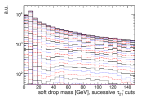
In order to distinguish hadronically decaying bosons (which give rise to jets that are intrinsically two-pronged) from QCD background, a flat cut on on is typically performed. As expected, this procedure greatly reduces the background, but it also leads to an unwanted sculpting of the soft drop jet mass distribution (an undesirable feature also discussed in Ref. Kasieczka:2015jma ), as shown in Fig. 1.
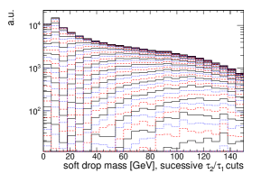
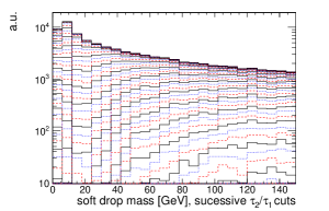
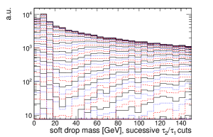
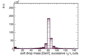
After cutting on to select jets which are two-pronged, the QCD background soft drop jet mass distribution becomes more peak-like in shape, making it harder to distinguish QCD jets from W jets which also have a peak in the jet mass distribution. The shape of the sculpted jet mass distribution, and the location of this artificial peak, varies for different jet regions. This dependent sculpting of the jet mass distributions makes sideband methods of background estimation more difficult. In this case and in further examples, we primarily consider gluon-initiated jets though performance with quark-initiated jets is similar. Differences will be explored in greater detail in future studies.
In Ref. Dasgupta:2013ihk it was argued that flat QCD mass distributions could be obtained by tuning the value of the soft drop energy fraction threshold (), and optimal values for quark- and gluon-initiated jets were analytically derived. However, the presence of the cut makes this situation more complex and it requires reconsidering the issue.
Therefore, we propose additional criterion in determining a better tagging observable beyond pure statistical discrimination power. For similarly discriminant observables, we would like to find an observable which is (1) primarily uncorrelated with the groomed jet mass observable (or rather that has complementary correlations as far as discrimination is concerned) and (2) maintains a desirable groomed mass behavior while scaling . Observables satisfying this criterion would, after applying a rectangular cut, still produce a flat groomed jet mass distribution.
3 Shape observable scaling in QCD
We start our study of the correlations of substructure variables with the jet mass and by introducing the appropriate scaling variable for QCD jets:
| (1) |
Here we have differed from the typical definition of jet by removing the jet distance parameter from the denominator of the definition. For now we keep fixed and leave this for future study. Note that when we apply soft-drop, we take the mass in Eq. (1) to be computed on the constituents of the soft-drop jet, while the transverse momentum is the one of the original (ungroomed) jet.
We now compute, on both our background and signal samples, the average value of the -subjettiness ratio (computed on the full jet) as a function of the soft-drop . This is shown in Fig. 2, on the left. The signal W jets are shown in open circles while the background, here gluon jets, are shown in closed circles. The various colors are different bins in jet . We note the typical behavior showing for the signal tending to lower values than the background and at a given value in due to the mass scale of the signal jet in a given bin. The signal tends to be fixed around the W mass and thus shifts for different values of and is otherwise most concentrated in the dip region. Now, let us focus on the background curves (solid points). We notice a strong dependence on which is what causes the sculpting of the mass distributions shown in the previous section. However, we note that there exist a region in for which this relationship is conspicuously linear. This is an interesting behavior, which we will exploit shortly in Sec. 4. We also observe that, even in this linear region, there is still a residual dependence, which looks like, to a very good approximation, a constant shift. The behavior observed in Fig. 2 for soft drop is also observed for other groomers, such as trimming and pruning, within the ranges consdidered. At lower values of differences in the groomers become more apparent, most likely because in that region trimming and pruning acquire further sensitivity to soft physics Dasgupta:2013ihk . Thus, in the current study, we concentrate on the soft-drop mass due to its stable behavior.
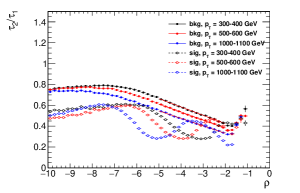
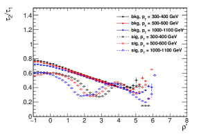
This approximate linear relation between can be (qualitatively) understood by noting that, in the case , essentially measures the subjet mass, while corresponds to the jet mass itself. This leads to an approximately linear relation between and in the region of the (soft-collinear) phase-space where all-order effects can be neglected.111We thank Andrew Larkoski for raising this point. Furthermore, Ref. Dasgupta:2015lxh performed calculations for jet mass distributions in the presence of a cut to an accuracy which is close to next-to-leading logarithmic (NLL) accuracy. Despite the fact that the calculation corresponding to the profile plot in Fig. 2 were not performed, it could in principle be derived because the authors do provide the double differential distribution in and . However, some important differences between our current set-up and the one of Ref. Dasgupta:2015lxh prevent us from using their results to get more quantitative insight in the behaviors we observe beyond the existence of a region with linear correlation. First Ref. Dasgupta:2015lxh did not consider the soft drop and, second, the definition of -subjettiness differs in the two studies both in regards of the angular exponent ( versus ) and of the choice of axes. We note that, at fixed-coupling, all the transverse momentum dependence is accounted for in the definition of the shape and . We have checked whether the origin of the dependence that we see in Fig. 2 (on the left) could be traced back to the transverse momentum used in the definition of the (ungroomed vs groomed) but this was found not to be the case. Running coupling contributions, as well as other subleading corrections, do introduce a dependence and they are likely to responsible for the observed dependence. However, a quantitative understanding of these effects would require a calculation using the techniques of Ref. Dasgupta:2015lxh . This goes beyond the scope of this work and for this study we limit ourselves to a phenomenological solution, while leaving a first-principle analysis for future work. Thus, in order to remove the constant dependence in the profile, we introduce a modified version of :
| (2) |
This change of variable, together with the choice GeV, appears to perform an excellent job in getting rid of the dependence, as shown in Fig. 2, on the right, though of course we note this is purely an empirical observation.
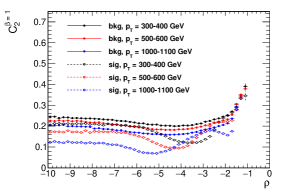
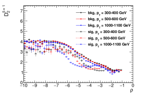
So far, we have only considered versus soft drop mass. We also noted that a similar linear correlation exists between and other groomed masses, though not shown explicitly. We can also consider other shape variables, though we leave an exhaustive exploration of all shape variables to a later study. As an example, we show also energy correlation functions and as a function of in Fig. 3. On the left, shows a relatively flat distribution versus which is desirable although the behavior is not quite linear. On the right, is highly correlated with . In both cases, the correlations have some -dependence that is not trivially empirically determined.
4 Designing decorrelated taggers (DDT)
4.1 Transforming
By performing the transformation , we have successfully accounted for most of the dependence of the profile distribution. Next we would like to perform a further transformation with the aim of flattening the profile dependence on , with the idea that this will in turn reduce the mass-sculpting discussed earlier.
In order to determine the transformation we are after, we concentrate on the region in which the relationship between and is essentially linear. Thus, we introduce
| (3) |
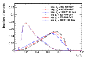
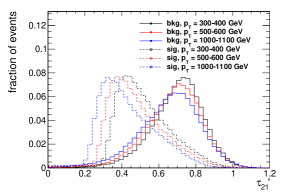
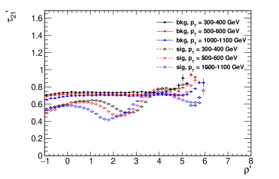
where the slope is numerically fitted from Fig. 2 (red fit lines). The comparison between the and distributions is shown in Fig. 4, for different jet bins. The transformed variable, , looks similar to the original variable although the behavior of the correlation with the groomed mass is now practically removed. We note that a -dependence on the signal shape is introduced which is, in hindsight, expected given the transformation takes advantage of scaling properties of the background. This can cause a -dependence in the signal efficiency with a cut on not present in the original ; however, we note this is not necessarily an undesirable feature. For example, as backgrounds decrease at higher it may be desirable to allow a larger signal efficiency and this should be studied in more detail in the experiments within the context of particular analyses. This can be seen in Fig. 5 which shows the profile of as a function of with the intended decorrelated behavior.
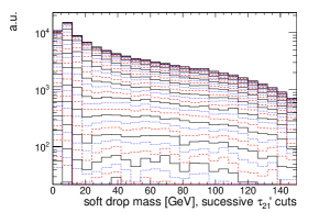
Now, we can explore the sculpting of the mass distributions making a flat cut in . This is shown in Fig. 6 which should be contrasted with Fig. 1 which was obtained with a flat cut in . Notice that now the sculpting of the mass distribution is considerably reduced, particularly in the region of interest where the boson peak is.
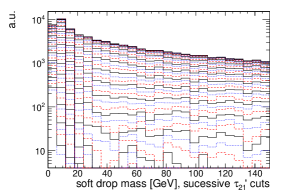
With a simple transformation, we can now preserve mass sidebands for background estimations and make robust predictions of the dependence of the backgrounds. This practical consequences of a well-behaved background shape will be explored in Section 5. Generally speaking, a non-linear dependence is not a technical obstacle to performing an observable transformation and we discuss this in Section 6; however, studying the behavior in a simple analytic regime allows us to better understand the underlying physical behavior. The final component to evaluating the success of the observable transformation is to understand the performance of the new observable in terms of rejecting backgrounds.
4.2 Performance of DDT
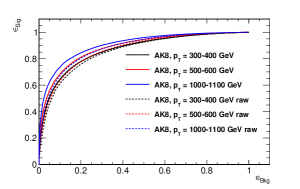
To evaluate the performance of the transformed variable we use the traditional receiver operating characteristic (ROC) curve, defined as the signal efficiency as a function of the background efficiency. A better discriminating tagger is characterized by higher signal efficiency and lower background efficiency. The discriminating performance of and the transformed are shown in the left of Fig. 7 for jets within a soft drop mass window of [60-120] GeV (corresponding to the signal mass region). From the ROC curve, we note that after transforming the variable the discriminating power does not degrade and even shows modest improvement in this kinematic regime. We can see where this comes from in the right panel of Fig. 7. After cutting on raw the QCD soft drop jet mass distribution is sculpted such that many of the jets surviving the cut fall into the W mass region. In contrast, cutting on leaves a more linearly falling distribution which preserves the low sideband. The mass distributions on the right side of Fig. 7 are after making a cut on the shape observable to maintain a signal efficiency of 50%.
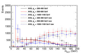
5 Case studies
Currently, the systematic uncertainties in extracting the efficiency are large (and usually dominant) sources of uncertainty in SM and BSM analyses at the LHC Khachatryan:2015bma ; Khachatryan:2015ywa ; Khachatryan:2014gha ; Khachatryan:2014hpa ; Chatrchyan:2012ypy ; Aad:2015owa ; Aad:2015uka . There are several places where the improved scaling behavior can reduce these systematics, in addition to the performance improvements in the ROC curves shown in Fig. 7. We will present two improvements, the preservation of mass sidebands in the kinematic fit to extract the tagging efficiency from semileptonic events, and the overall background estimate in diboson analyses. Both cases take advantage of the flatter background distributions to improve the uncertainties in shape-based fits.
5.1 Preservation of mass sidebands
The shape of the jet mass spectrum is used in the LHC experiments to determine the tagging efficiency; for instance, CMS relies on a simultaneous fit to the jet mass in events that pass and fail the selection. However, as shown in Fig. 1, the selection significantly kinematically sculpts the background distribution in this variable. This can lead to significant fitted uncertainties when extracting the background normalization, and thus directly translates to large uncertainties in the tagging efficiency measurement. By using the , a significant improvement is observed.
To demonstrate this, we examine two cases, modified mass drop tagging with , and modified mass drop tagging with a scale-dependent selection , where . This translates into a cut on . These selections have approximately the same signal efficiency. For simplicity, the same signal and background MC samples are used as in the previous sections, but the events are weighted with an easily specifiable fraction of background jets. In this case, the background fraction for the entire sample is 40%. This gives a comparable fraction of merged to unmerged bosons in a semileptonic selection at 13 TeV at the LHC, but allows us to easily tune the fraction. In addition, to mimic the approximate detector resolution, the intrinsic resolution of the system is smeared with a Gaussian of width 10 GeV. This is indicative of the resolutions obtained at the CMS and ATLAS experiments.
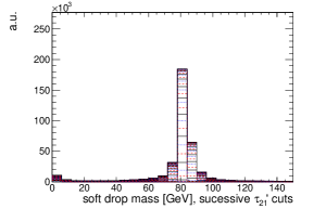
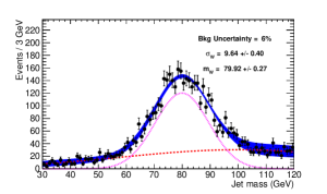
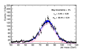
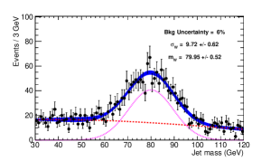
Figure 8 shows simple fits to the jet mass for 5000 MC events in the range GeV, after a selection on the -subjettiness variable. The model is a double Gaussian, one for the QCD continuum and one for the mass peak. The jet range considered is GeV, to give a typical range of the bosons from top quark decays from SM production. The first fit shows the modified mass drop algorithm after . The second fit shows the modified mass drop algorithm after . The fits successfully capture the mass of the and the input width of 10%.
It is interesting to note that the jet mass of the QCD jets after the selection are significantly pushed below 10 GeV. In addition, the remaining distribution is flat. However, for the standard selection, the distribution is rising, with significantly more background under the signal peak.
The background uncertainty on the fit is is 6% when using the standard selection. However, it is reduced by a factor of two to 3% by using the selection. This is driven by the fact that the fitter can more easily handle sidebands that are flatter, so the variable outperforms the variable in this metric.
This would translate directly into a decreased systematic uncertainty for the LHC experiments. While newer and more clever algorithms can achieve better performance in MC simulations, this does not always translate directly to improvements in actual analyses due to the need to characterize the systematic uncertainties. We therefore propose this test as an appropriate metric to characterize the systematic performance of new substructure algorithms.
5.2 Diboson Background Estimate
The diboson background estimate for the LHC experiments is much the same as the extraction of the tagging efficiency, except that the background fraction is significantly higher. We have chosen a value of 80% (integrated over the entire spectrum of events) as an indicative fraction, with the same number of events (5000). We have considered two different ranges, GeV and GeV.
One somewhat obvious but important point is that as the increases, the Sudakov peak from QCD-generated jets shifts further to the right. As this occurs, the fits to discriminate boosted bosons from QCD-generated jets are less and less able to distinguish between the categories.
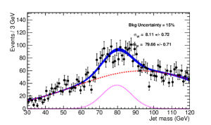
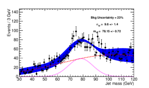
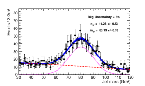
Figures 9 and 10 show similar fits as shown in Fig. 8. However, the background fraction is raised from 40% to 80% (again integrated over the entire mass spectrum), and the ranges are set to GeV and GeV, respectively.
For the range GeV, it is plain to see that there is a significant improvement of the variable, where the background uncertainty decreases from 15% to 6%. This is even more apparent for the range GeV,where the uncertainty decreases from 23% to 6%.
6 Generalized Scale Invariance
Decorrelation schemes can be extended beyond a pair of variables to decorrelate classes of many variables. Such a procedure can be used to allow for a class of variables to be merged into a single multi-variate analysis discriminator (MVA), while preserving decorrelation against one or a set of variables that are further used in the analysis. Consider, for example, building an MVA tagger using both and . Both of these variables have correlations with and mass, so the resulting classifier that combines the variables will also be correlated with mass and . Decorrelating the space of variables against mass and before or during the construction of the MVA can thus preserve the mass and invariance resulting in an uncorrelated tagger. This idea has previously been pursued in -physics utilizing an MVA that minimizes the mass dependence, while simultaneously constructing a classifier Rogozhnikov:2014zea .
In light of building an example based on previously presented studies, we split by into it components and . Combining this with either or gives a class of three variables for which we decorrelate into a set of three independent linear combinations of variables. The independent variables can be viewed as properties of the data which span the space of distinctive features. This space can be explored to further understand behavior of the data. Additionally, a subset of the independent components can be merged through an MVA while maintaining the decorrelation of the remaining set of variables. In this way, mass sidebands or other sideband methods can be used on the merged MVA discriminator with the decorrelated variable.
As has previously been noted, decorrelating variables which are not implicitly linearly correlated is poorly defined Larkoski:2014pca . We thus consider two generalized approaches that attempt to decorrelate discriminators that are not necessarily linearly correlated. We consider two decorrelation approaches: Principle Component Analysis (PCA) of transformed variables and Independent Component Analysis (ICA).
Decorrelation by PCA and ICA
Given a set of variables need not be linearly correlated, we consider a transformed variable () of the original variable defined by
| (4) |
For this transformation, we train a gradient boosted decision tree Hocker:2007ht with the boosted boson as a signal and a high QCD jet as a background. This transformation places the variables into a space that enables the possibility of linearized correlations of the original variables.
The resulting correlation matrix of the transformed variables can be decorrelated through principle component analysis by taking the eigenvectors of the matrix. This yields a set of -independent vectors for a -dimensional correlation matrix.
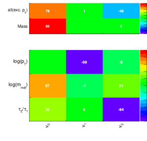
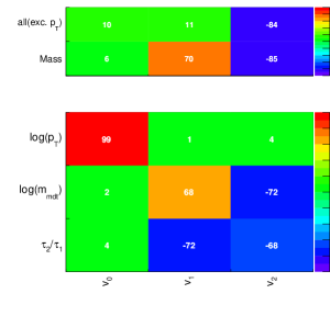
The decorrelated vectors for the triplet of transformed , , and is shown in Fig. 11. The correlation of the resulting vectors is compared with a gradient boosted decision tree using all variables and with the transformed mass. From this correlation, we observe two discriminating dimensions and the . These we can write as
| (5) | |||||
| (6) |
where correspond to coefficients and are scales, typically GeV to make the observables dimensionless. The first variable corresponds to the transformed mass and the second corresponds the transformed . The second variable is not too different from decorrelated .
An alternative decorrelation approach, known as independent component analysis (ICA), involves diagonalization of the matrix constructed by computing the pairwise mutual information of each pair of variables on the sample of QCD jets. This differs to previous approaches, which rely on the mutual information to truth. Here, we focus on identifying features in the data and not necessarily discriminating power. We perform the ICA with an algorithm that uses -nearest neighbor to expedite the diagonalization process (MILCA) kraskov:2004 . The right panel of Fig. 11 shows the ICA decomposed vectors. As with the transformed PCA, the ICA decorrelates the , however the mass interdependence is stronger than in the transformed case.
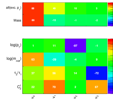
Finally, the equivalent decorrelated matrix for a combined set of observables is shown in Fig. 12, here we show just the transformed PCA approach. From the combined set, we observe the largest orthogonal set of discrimination power comes from the as oppose to . When comparing the two approaches, we have found variable transformed PCA yields a more consistent performance with our previous observations.
7 Conclusion and Outlook
In this note, we explore the scale-dependence and correlations of jet substructure observables. The goal is not only to improve the statistical power of such observables, which we also demonstrate, but also to consider practical issues related to using such observables in searches for new physics. In order to design decorrelated taggers (DDT), we transform the shape observable, here , by decorrelating it from groomed mass observables also factoring in the scale-dependence. In addition to improving the statistical discrimination between signal and background, we also preserve a robust, flat background shape and which has more stable behavior when scaling of the background going from lower bins to higher bins. We demonstrate the advantages of such an approach in various case studies such as predicting background normalizations and determining heavy object tagging scale factors related to new physics searches.
The intention of this note is not to perform a detailed study of all possible heavy object taggers, but instead, to introduce further considerations when designing taggers and propose a method by which all considerations can be addressed, namely via observable decorrelation. We leave studies related to variations on jet mass groomers and shape observables, R-scaling, quark-gluon fractions, scaling background predictions, behavior at extremely high , and top tagging to future works. We have explored more generic determinations of observable decorrelation with complex taggers using multivariate techniques and numerical principle-component analysis.
Acknowledgments
We thank Andrew Larkoski and Petar Maksimovic for their critical reading of the manuscript. The authors would also like to thank Matteo Cremonesi, Matthew Low, Cristina Mantilla Suarez, Siddharth Narayanan, Gavin Salam, Gregory Soyez, and Michael Spannowsky for useful discussion and inputs. JD and SR are partially supported by the U.S. National Science Foundation, under grant PHY–1401223. PH is supported by CERN. The work of SM is partly supported by the U.S. National Science Foundation, under grant PHY–0969510, the LHC Theory Initiative. NT is supported by the Fermi Research Alliance, LLC under Contract No. De-AC02-07CH11359 with the United States Department of Energy.
References
- (1) A. Abdesselam, E. B. Kuutmann, U. Bitenc, G. Brooijmans, J. Butterworth, et al., Boosted objects: A Probe of beyond the Standard Model physics, Eur. Phys. J. C 71 (2011) 1661, [arXiv:1012.5412].
- (2) A. Altheimer, S. Arora, L. Asquith, G. Brooijmans, J. Butterworth, et al., Jet Substructure at the Tevatron and LHC: New results, new tools, new benchmarks, J. Phys. G 39 (2012) 063001, [arXiv:1201.0008].
- (3) A. Altheimer, A. Arce, L. Asquith, J. Backus Mayes, E. Bergeaas Kuutmann, et al., Boosted objects and jet substructure at the LHC. Report of BOOST2012, held at IFIC Valencia, 23rd-27th of July 2012, Eur.Phys.J. C74 (2014), no. 3 2792, [arXiv:1311.2708].
- (4) D. Adams et al., Towards an Understanding of the Correlations in Jet Substructure, Eur. Phys. J. C75 (2015), no. 9 409, [arXiv:1504.0067].
- (5) J. M. Butterworth, A. R. Davison, M. Rubin, and G. P. Salam, Jet substructure as a new Higgs search channel at the LHC, Phys. Rev. Lett. 100 (2008) 242001, [arXiv:0802.2470].
- (6) D. E. Kaplan, K. Rehermann, M. D. Schwartz, and B. Tweedie, Top Tagging: A Method for Identifying Boosted Hadronically Decaying Top Quarks, Phys. Rev. Lett. 101 (2008) 142001, [arXiv:0806.0848].
- (7) CMS Collaboration, A cambridge-aachen (c-a) based jet algorithm for boosted top-jet tagging, CMS Physics Analysis Summary CMS-PAS-JME-009-01, CERN, 2009.
- (8) S. D. Ellis, C. K. Vermilion, and J. R. Walsh, Techniques for improved heavy particle searches with jet substructure, Phys. Rev. D 80 (2009) 051501, [arXiv:0903.5081].
- (9) S. D. Ellis, C. K. Vermilion, and J. R. Walsh, Recombination Algorithms and Jet Substructure: Pruning as a Tool for Heavy Particle Searches, Phys. Rev. D 81 (2010) 094023, [arXiv:0912.0033].
- (10) D. Krohn, J. Thaler, and L. T. Wang, Jet Trimming, JHEP 02 (2010) 084, [arXiv:0912.1342].
- (11) J. Thaler and K. Van Tilburg, Maximizing Boosted Top Identification by Minimizing N-subjettiness, JHEP 1202 (2012) 093, [arXiv:1108.2701].
- (12) A. J. Larkoski, S. Marzani, G. Soyez, and J. Thaler, Soft Drop, JHEP 05 (2014) 146, [arXiv:1402.2657].
- (13) D. E. Soper and M. Spannowsky, Finding physics signals with shower deconstruction, Phys. Rev. D84 (2011) 074002, [arXiv:1102.3480].
- (14) D. E. Soper and M. Spannowsky, Finding top quarks with shower deconstruction, Phys. Rev. D87 (2013) 054012, [arXiv:1211.3140].
- (15) D. E. Soper and M. Spannowsky, Finding physics signals with event deconstruction, Phys. Rev. D89 (2014), no. 9 094005, [arXiv:1402.1189].
- (16) M. Dasgupta, A. Fregoso, S. Marzani, and G. P. Salam, Towards an understanding of jet substructure, JHEP 09 (2013) 029, [arXiv:1307.0007].
- (17) M. Dasgupta, A. Fregoso, S. Marzani, and A. Powling, Jet substructure with analytical methods, Eur.Phys.J. C73 (2013), no. 11 2623, [arXiv:1307.0013].
- (18) I. Feige, M. D. Schwartz, I. W. Stewart, and J. Thaler, Precision Jet Substructure from Boosted Event Shapes, Phys.Rev.Lett. 109 (2012) 092001, [arXiv:1204.3898].
- (19) M. Dasgupta, A. Powling, and A. Siodmok, On jet substructure methods for signal jets, JHEP 08 (2015) 079, [arXiv:1503.0108].
- (20) A. J. Larkoski, I. Moult, and D. Neill, Toward Multi-Differential Cross Sections: Measuring Two Angularities on a Single Jet, JHEP 1409 (2014) 046, [arXiv:1401.4458].
- (21) A. J. Larkoski, I. Moult, and D. Neill, Power Counting to Better Jet Observables, JHEP 12 (2014) 009, [arXiv:1409.6298].
- (22) A. J. Larkoski, I. Moult, and D. Neill, Building a Better Boosted Top Tagger, Phys. Rev. D91 (2015), no. 3 034035, [arXiv:1411.0665].
- (23) A. J. Larkoski, I. Moult, and D. Neill, Analytic Boosted Boson Discrimination, arXiv:1507.0301.
- (24) M. Dasgupta, L. Schunk, and G. Soyez, Jet shapes for boosted jet two-prong decays from first-principles, arXiv:1512.0051.
- (25) CMS Collaboration, V. Khachatryan et al., Identification techniques for highly boosted W bosons that decay into hadrons, JHEP 12 (2014) 017, [arXiv:1410.4227].
- (26) CMS Collaboration, Boosted Top Jet Tagging at CMS, Tech. Rep. CMS-PAS-JME-13-007, CERN, Geneva, 2014.
- (27) CMS Collaboration, V Tagging Observables and Correlations, Tech. Rep. CMS-PAS-JME-14-002, CERN, Geneva, 2014.
- (28) CMS Collaboration, Top Tagging with New Approaches, Tech. Rep. CMS-PAS-JME-15-002, CERN, Geneva, 2016.
- (29) ATLAS Collaboration, G. Aad et al., Performance of jet substructure techniques for large- jets in proton-proton collisions at = 7 TeV using the ATLAS detector, JHEP 09 (2013) 076, [arXiv:1306.4945].
- (30) ATLAS Collaboration, G. Aad et al., Identification of Boosted, Hadronically Decaying W Bosons and Comparisons with ATLAS Data Taken at TeV, arXiv:1510.0582.
- (31) Boosted hadronic top identification at ATLAS for early 13 TeV data, Tech. Rep. ATL-PHYS-PUB-2015-053, CERN, Geneva, Dec, 2015.
- (32) Identification of boosted, hadronically-decaying and bosons in TeV Monte Carlo Simulations for ATLAS, Tech. Rep. ATL-PHYS-PUB-2015-033, CERN, Geneva, Aug, 2015.
- (33) J. Cogan, M. Kagan, E. Strauss, and A. Schwarztman, Jet-Images: Computer Vision Inspired Techniques for Jet Tagging, JHEP 02 (2015) 118, [arXiv:1407.5675].
- (34) L. G. Almeida, M. Backovi?, M. Cliche, S. J. Lee, and M. Perelstein, Playing Tag with ANN: Boosted Top Identification with Pattern Recognition, JHEP 07 (2015) 086, [arXiv:1501.0596].
- (35) L. de Oliveira, M. Kagan, L. Mackey, B. Nachman, and A. Schwartzman, Jet-Images – Deep Learning Edition, arXiv:1511.0519.
- (36) J. Alwall, R. Frederix, S. Frixione, V. Hirschi, F. Maltoni, O. Mattelaer, H. S. Shao, T. Stelzer, P. Torrielli, and M. Zaro, The automated computation of tree-level and next-to-leading order differential cross sections, and their matching to parton shower simulations, JHEP 07 (2014) 079, [arXiv:1405.0301].
- (37) Y. Gao, A. V. Gritsan, Z. Guo, K. Melnikov, M. Schulze, and N. V. Tran, Spin determination of single-produced resonances at hadron colliders, Phys. Rev. D81 (2010) 075022, [arXiv:1001.3396].
- (38) T. Sjöstrand, S. Mrenna, and P. Skands, A brief introduction to PYTHIA 8.1, Comput. Phys. Commun. 178 (2008) 852–867, [arXiv:0710.3820].
- (39) A. Buckley et al., General-purpose event generators for LHC physics, Phys. Rept. 504 (2011) 145–233, [arXiv:1101.2599].
- (40) M. Cacciari, G. P. Salam, and G. Soyez, The anti-kt jet clustering algorithm, JHEP 04 (2008) 063, [arXiv:0802.1189].
- (41) M. Cacciari and G. P. Salam, Dispelling the N**3 myth for the k(t) jet-finder, Phys. Lett. B 641 (2006) 57–61, [hep-ph/0512210].
- (42) M. Cacciari, G. P. Salam, and G. Soyez, FastJet User Manual, Eur. Phys. J. C72 (2012) 1896, [arXiv:1111.6097].
- (43) ATLAS Collaboration, G. Aad et al., Jet mass and substructure of inclusive jets in TeV collisions with the ATLAS experiment, JHEP 1205 (2012) 128, [arXiv:1203.4606].
- (44) CMS Collaboration, S. Chatrchyan et al., Studies of jet mass in dijet and W/Z+jet events, JHEP 1305 (2013) 090, [arXiv:1303.4811].
- (45) G. Kasieczka, T. Plehn, T. Schell, T. Strebler, and G. P. Salam, Resonance Searches with an Updated Top Tagger, JHEP 06 (2015) 203, [arXiv:1503.0592].
- (46) CMS Collaboration, V. Khachatryan et al., Search for a massive resonance decaying into a Higgs boson and a W or Z boson in hadronic final states in proton-proton collisions at TeV, JHEP 02 (2016) 145, [arXiv:1506.0144].
- (47) CMS Collaboration, V. Khachatryan et al., Search for Narrow High-Mass Resonances in Proton–Proton Collisions at = 8 TeV Decaying to a Z and a Higgs Boson, Phys. Lett. B748 (2015) 255–277, [arXiv:1502.0499].
- (48) CMS Collaboration, V. Khachatryan et al., Search for massive resonances decaying into pairs of boosted bosons in semi-leptonic final states at 8 TeV, JHEP 08 (2014) 174, [arXiv:1405.3447].
- (49) CMS Collaboration, V. Khachatryan et al., Search for massive resonances in dijet systems containing jets tagged as W or Z boson decays in pp collisions at = 8 TeV, JHEP 08 (2014) 173, [arXiv:1405.1994].
- (50) CMS Collaboration, S. Chatrchyan et al., Search for heavy resonances in the W/Z-tagged dijet mass spectrum in pp collisions at 7 TeV, Phys. Lett. B723 (2013) 280–301, [arXiv:1212.1910].
- (51) ATLAS Collaboration, G. Aad et al., Search for high-mass diboson resonances with boson-tagged jets in proton-proton collisions at TeV with the ATLAS detector, JHEP 12 (2015) 055, [arXiv:1506.0096].
- (52) ATLAS Collaboration, G. Aad et al., Search for Higgs boson pair production in the final state from pp collisions at TeVwith the ATLAS detector, Eur. Phys. J. C75 (2015), no. 9 412, [arXiv:1506.0028].
- (53) A. Rogozhnikov, A. Bukva, V. Gligorov, A. Ustyuzhanin, and M. Williams, New approaches for boosting to uniformity, JINST 10 (2015), no. 03 T03002, [arXiv:1410.4140].
- (54) A. J. Larkoski, J. Thaler, and W. J. Waalewijn, Gaining (Mutual) Information about Quark/Gluon Discrimination, JHEP 11 (2014) 129, [arXiv:1408.3122].
- (55) A. Hoecker, P. Speckmayer, J. Stelzer, J. Therhaag, E. von Toerne, and H. Voss, TMVA: Toolkit for Multivariate Data Analysis, PoS ACAT (2007) 040, [physics/0703039].
- (56) A. Kraskov, H. Stögbauer, and P. Grassberger, Estimating mutual information, Phys. Rev. E 69 (Jun, 2004) 066138.