Bayesian Variable Selection for Skewed Heteroscedastic Response

Abstract

In this article, we propose new Bayesian methods with proper theoretical justification for selecting and estimating a sparse regression coefficient vector for skewed heteroscedastic response. Our novel Bayesian procedures effectively estimate the median and other quantile functions, accommodate non-local prior for regression effects without compromising ease of implementation via sampling based tools. First time for skewed and heteroscedastic response, this Bayesian method asymptotically selects the true set of predictors even when the number of covariates increases in the same order of the sample size. We also extend our method to deal with some observations with very large errors. Via simulation studies and a re-analysis of a medical cost study with large number of potential predictors, we illustrate the ease of implementation and other practical advantages of our approach compared to existing methods for such studies.

Keywords: Bayesian consistency; median regression; sparsity

1 Introduction

Large number of possible predictors and highly skewed heteroscedastic response are often major challenges for many biomedical and econometric applications. Selection of an optimal set of covariates and subsequent estimation of the regression function are important steps for scientific conclusions and policy decisions based on such studies. For example, previous analyses of Medical Expenditure Panel Study (Natarajan et al., 2008; Cohen, 2003) testify to the highly skewed and heteroscedastic nature of the main response of interest, total health care expenditure in a year. Also, it is common in such studies to have a small proportion of patients with either very high or very low medical costs. Popular classical sparse-regression methods such as Lasso (Least absolute shrinkage operator) by Tibshirani (1996) and Efron et al. (2004), and later related methods of Fan and Li (2001), Zou and Hastie (2005), Zou (2006) and MCP (Zhang, 2010) assume Gaussian (or, at least symmetric) response density with common variance. Limited recent literature on consistent variable selection for non-Gaussian response includes Zhao and Yu (2006) under common variance assumption, Bach (2008) under weak conditions on covariate structures, and Chen et al. (2014) under skew-t errors. However, none of these methods deal with estimation of quantile function for heteroscedastic response frequently encountered in complex biomedical studies. Many authors including Koenker (2005) argue effectively against focusing on mean regression for skewed heteroscedastic response. Our simulation studies demonstrate that directly modeling skewness and heteroscedasticity, particularly in presence of analogous empirical evidence, leads to better estimators of quantile functions for finite samples compared to existing methods which ignore skewness and heteroscedasticity.

Bayesian methods for variable selection have some important practical advantages including incorporation of prior information about sparsity, evaluation of uncertainty about the final model, interval estimate for any coefficient of interest, and evaluation of the relative importance of different coefficients. Asymptotic properties of Bayesian variable selection methods when the number of potential predictors, $p$, increases as a function of sample size $n$ have received lot of attention recently in the literature. Traditionally, to select the important variables out of $(X_{1},\ldots,X_{p})$, a two component mixture prior, also referred to as “spike and slab” prior, (Mitchell and Beauchamp, 1988; George and McCulloch, 1993, 1997) is placed on the coefficients $\beta=(\beta_{1},\ldots,\beta_{p})$. These mixture priors include a discrete mass, called a “spike”, at zero to characterize the prior probability of a coefficient being exactly zero (that is, not including the corresponding predictor in the model) and a continuous density called a “slab”, usually centered at null-value zero, representing the prior opinion when the coefficient is non-zero. Following Johnson and Rossell (2010a, b), when the continuous density of the slab part of a spike and slab prior has value 0 at null-value 0, we will call it a non-local mixture prior. Continuous analogues of local mixture priors are being proposed recently by Park and Casella (2008); Carvalho et al. (2010); Bhattacharya et al. (2014) among others. Bondell and Reich (2012) presented the selection consistency of joint Bayesian credible sets. However, current Bayesian variable selection methods usually focus on mean regression function for models with symmetric error density and common variance.

Johnson and Rossell (2010b) recently showed a startling selection inconsistency phenomenon for using several commonly used mixture priors, including local mixture (spike and slab prior with non-zero value at null-value 0 of the slab density) priors, when $p$ is larger than the order of $\sqrt{n}$. To address this for mean regression with sparse $\beta$, they advocated the use of non-local mixture density presenting continuous “slab” density with value 0 at null-value 0 because these priors, called non-local mixture priors here, obtain selection consistency when the dimension $p$ is $O(n)$. Castillo et al. (2014) provided several conditions to ensure selection consistency even when $p\gg n$. However, none of these Bayesian methods specifically deal with skewed and heteroscedastic response, contamination of few observations with large errors and variable selection for median and other quantile functionals.

In this article, we accommodate skewed and heteroscedastic response distribution using transform-both-sides model (Lin et al., 2012) with sparsity inducing prior for the vector of regression coefficients. Our key observation is that, under such models with generalized Box-Cox transformation (Bickel and Doksum, 1981), even a local mixture prior on after-transform regression coefficients induces non-local priors on the original regression function for certain choices of the transformation parameter. Similar to moment and inverse moment non-local priors in Johnson and Rossell (2010b), this method enables clear demarcation between the signal and the noise coefficients in the posterior leading to consistent posterior selection even when $p=O(n)$. Addition to that, our use of standard local priors on the transformed regression coefficients facilitates straightforward posterior computation which can be implemented in publicly available softwares. We later extend this model to accommodate cases when the observations are contaminated with a small number of observations with very large (or small) errors. Our approaches are shown to out-perform well-known competitors in simulation studies as well as for analyzing and interpreting a real-life medical cost study.

2 Bayesian variable selection model

2.1 Transform-both-Sides Model

For the skewed and heteroscedastic response $Y_{i}$ for $i=1,\ldots,n$, we assume the transform-both-sides model (Lin et al., 2012)

$$g_{\eta}(Y_{i})=g_{\eta}(x_{i}^{T}\beta)+e_{i}\ ,$$ (1)

where $\beta=(\beta_{1},\ldots,\beta_{p})^{\prime}$, $x_{i}$ is the observed $p$-dimensional covariate vector, $g_{\eta}(y)$ is the monotone power transformation (Bickel and Doksum, 1981),

$$g_{\eta}(y)=\frac{y|y|^{\eta-1}-1}{\eta},$$ (2)

with unknown parameter $\eta\in(0,2)$. This transformation in (2) is an extension of Box-Cox power family that has a long history and success in dealing with skewed and heteroscedastic response. We assume that under an optimal $\eta$, the transformed response $g_{\eta}(y)$ has a symmetric and unimodal distribution with mean and median $g_{\eta}(x_{i}^{T}\beta)$. Thus $e_{i}$’s are independent mean 0 errors with common symmetric density function $f_{e}$ and variance $\sigma^{2}$. The transformation $g_{\eta}(y)$ in (2) is monotone with derivative $g_{\eta}^{\prime}(y)=|y|^{\eta-1}\geq 0$. Model (1) can be expressed as a linear model

$$Y_{i}\ =\ x_{i}^{T}\beta\ +\ \epsilon_{i}\ ,$$ (3)

where $\epsilon_{i}$ has a skewed heteroscedastic density with median 0 because $P[\epsilon_{i}>0]=1/2$, and approximate variance is $\sigma^{2}|x_{i}^{T}\beta|^{2-2\eta}$. Hence, the median of the skewed and heteroscedastic response $Y_{i}$ in (1) is $x_{i}^{T}\beta$. For the time being, we consider a Gaussian $\mbox{N}(0,\sigma^{2})$ density for $f_{e}$ in (1). Later in §4, we consider other densities to accommodate a heavy tail for $f_{e}$.

For the model of (1), any sparsity inducing prior for $\beta$ should depend on the transformation parameter $\eta$ since $\eta$ has a significant effect on the range and scale of $Y_{i}$ (approximate variance $\sigma^{2}|x_{i}^{T}\beta|^{2-2\eta}$). Based on this argument, we specify an conditional mixture prior $g_{\eta}(\beta_{j})$ given $\eta$ using a “local” $\phi(\cdot;0,\sigma_{\beta}^{2})$ density for the “slab” when $g_{\eta}(\beta_{j})$ is non-zero with discrete prior probability $(1-\pi_{0})$, where $\phi(\cdot;\mu,v^{2})$ is the Gaussian density with mean $\mu$ and variance $v^{2}$. This conditional mixture prior $g_{\eta}(\beta_{j})$ given $\eta$ (a local mixture prior according to definition of Johnson and Rossell (2010b)) results in a conditional mixture prior

$$f_{\beta}(\beta_{j}\mid\eta)=\pi_{0}\delta_{0}(\beta_{j})+(1-\pi_{0})\phi(g_{\eta}(\beta_{j});0,\sigma_{\beta}^{2})|g_{\eta}^{\prime}(\beta_{j})|$$ (4)

for $\beta_{j}$ given $\eta$ independently for $j=1,\cdots,p$, where $\pi_{0}\in[0,1]$ is the probability of $\beta_{j}$ being zero, $\delta_{0}(\cdot)$ is the discrete measure at 0. When $\eta>1$, $g_{\eta}^{\prime}(0)=0$ and hence the resulting unconditional marginal prior for the nonzero $\beta_{j}$ in (4) turns out to be a non-local mixture prior of Johnson and Rossell (2010b). However, the prior of transformed $g_{\eta}(\beta_{j})$, a mixture of discrete measure at 0 and $\phi(\cdot;0,\sigma_{\beta}^{2})$ density, is a local mixture prior. This is demonstrated via the plots of two resulting unconditional priors of $\beta_{j}$ when $\eta=0.5$ and $\eta=1.5$ in Figure 1. Our simulation study in §5 shows that the model selection and estimation procedures for our Bayesian method perform substantially better than competing methods when $\eta>1$ (case with non-local unconditional prior for $\beta_{j}$) compared to, say, when $\eta=0.5\in(0,1)$ (case with a local prior for $\beta$ given $\eta$). Thus, heteroscedasticity and the possibly non-local property of $\pi(\beta\mid\eta)$ come as a bi-product of the transform-both-sides model of (1). This implicit non-local mixture prior modeling of unconditional $\beta_{j}$ may be the reason for some desirable asymptotic properties of our method even when $p=O(n)$ (discussed in §3). However, our methods’ ability to use a local prior for $g_{\eta}(\beta_{j})$ significantly reduces computational complexity of the associated Markov chain Monte Carlo (MCMC) algorithms, while facilitating the desirable asymptotic property.

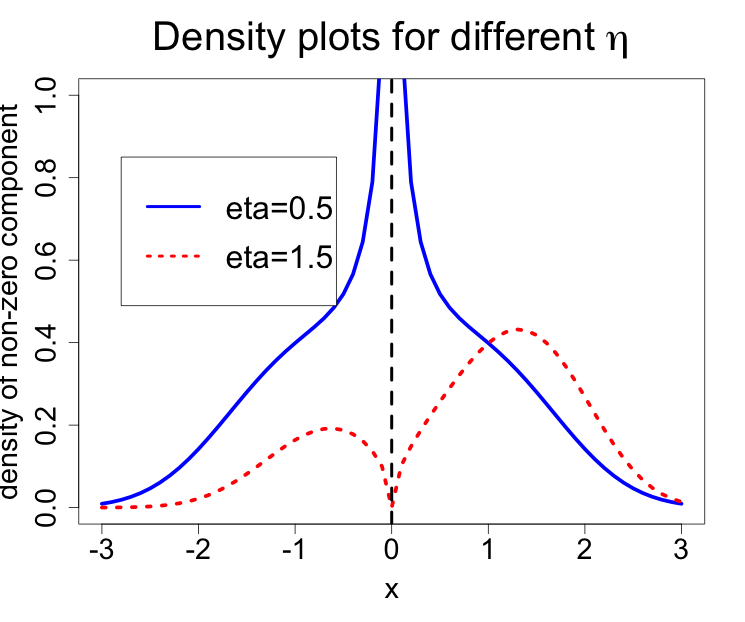
Figure 1: Density Plot for Different $\eta$

When the error density $f_{e}$ in (1) is Gaussian $\phi(\cdot;\mu,\sigma^{2})$ with mean 0 and variance $\sigma^{2}$, we can specify a hierarchical Bayesian model using the prior $\pi(\beta\mid\eta)$ in (1) along with known priors for $\sigma^{2}$ and $\eta$,

$$\sigma^{2}\sim\mbox{IGa}(a,b),\quad\eta/2\sim\mbox{Beta}(c_{1},d_{1})$$ (5)

and a hyperprior for the hyperparameters $(\pi_{0},\sigma_{\beta}^{2})$. For computational simplicity, in §3, we establish variable selection consistency of this hierarchical Bayesian model using (1) along with the non-local prior (4) on $\beta$ and the prior for $\sigma^{2}$ in (5).

3 Consistent variable selection for large $p$

In this section, we investigate selection consistency of the proposed model when the number of covariates $p$ is grows with sample size $n$, with $p\leq n$ and the true error density is skewed and heteroscedastic, but follows the same specification as in (1). Unlike the Gaussian likelihood with mixture priors of Johnson and Rossell (2010b), our Bayesian model described in (1) - (5) does not admit a closed form expression of the marginal likelihood. We derive appropriate bounds of the marginal likelihood to obtain the desired Bayesian consistency results. Here we only present a brief outline of our assumptions, developments and practical implications of our theoretical results. Supporting results and details of the proofs are deferred to §Proof of Theorem 1. For brevity of exposition, we consider a design matrix $X$ which are nearly orthogonal in the sense that there exists constant $0<c_{1}\leq c_{1}$ such that $c_{1}n\leq\lambda_{1}(X^{T}X)\leq\lambda_{p}(X^{T}X)\leq c_{2}n$ where $\lambda_{1}(A)\leq\lambda_{2}(A)\leq\cdots\leq\lambda_{p}(A)$ denote ordered eigen values of the matrix $A$. The assumption ensures identifiability of the regression coefficient $\beta$ and is commonly assumed in the selection consistency literature, refer for example to Johnson and Rossell (2010b).

To estimate the posterior probability assigned to the correct model, we use Laplace approximation (Rossell and Telesca, 2015) to obtain probabilistic bounds of marginal likelihood $p(y|\gamma)$. Here $\gamma=(\gamma_{1},\ldots,\gamma_{p})$ denotes the predicted model for which $\gamma_{j}=I(\beta_{j}\neq 0)$ for $j=1,2,\cdots,p$ are the indicators of active coefficients and $p_{\gamma}=\sum_{i=1}^{p}\gamma_{i}$ denotes the number of active variables. Denote by $\beta^{*}$ the vector of true regression coefficients with $\gamma^{*}$ defined accordingly. Assuming $\tilde{\beta}$ as the posterior mode and $\eta$ is the optimal power parameter, the Laplace approximation of $p(y|\gamma)$ around $\tilde{\beta}$ is

$$p(y|\gamma)\approx\frac{(2\pi)^{p_{\gamma}/2}}{|H(\tilde{\beta})|^{1/2}}\exp\{\log L(\tilde{\beta})+\text{log}(\pi(\tilde{\beta}|\gamma)))\}$$ (6)

where the projection of the prior $f_{\beta}$ in (4) onto the support of $\gamma$, denote by $\pi(\beta\mid\gamma)$ and is given as

$$\pi(\beta\mid\gamma)=\prod_{j\in\gamma}\phi(g_{\eta}(\beta_{j});0,\sigma_{\beta}^{2})\left\lvert g_{\eta}^{\prime}(\beta_{j})\right\rvert.$$ (7)

We note again that (7) becomes a non-local prior (Johnson and Rossell, 2010b) for $\eta\in(1,2)$ and is the primary reason for controlling false positives. Based on definitions of key concepts in (6) and (7), we state our main theorem on selection consistency of our Bayesian method even when $p$ is of the order $O(n)$.

Theorem 1

When the observations are generated from (1) for a known $\eta\in(1,2)$ and $\sigma>0$, and model (1) is fitted with priors (4) and (5) for the optimal $\eta$ and with any $\pi_{0}\in(0,1)$, then for $p\leq n$, the posterior probability $P(\gamma=\gamma^{*}\mid y)\to 1$ almost surely as $n,p\to+\infty$ .

The detailed proof of Theorem 1, given in §Proof of Theorem 1, is a non-trivial extension of the proof of Theorem 1 in Johnson and Rossell (2010b) which used non-local priors to obtain variable selection consistency. Unlike them, we use a local prior $g_{\eta}(\beta)$ to induce a possible non-local prior for $\beta$ given $\eta$ in (4). To the best of our knowledge, this is the first result on Bayesian selection consistency when the response distribution is skewed and heteroscedastic and our method of proof opens the theoretical investigation of sparse Bayesian methods for transformable models and heterodasticity.

4 Accommodating extremely large errors

Presence of few observations with extremely large errors and their influences on final analysis for various application areas have been emphasized by many authors including Hampel et al. (2011). The assumption of Gaussian error density $f_{e}$ in (1) may not be valid due to the presence of a small number of observations with large errors even after optimal Box-Cox transformation. To address this, we extend the model (1) to a random location-shift model with

$$g_{\eta}(Y_{i})=g_{\eta}(x_{i}^{T}\beta)+\gamma_{i}+e_{i}\ ,$$ (8)

where $\gamma_{i}$ is nonzero if the $i$th observation has large error, and zero otherwise. We assume the vector $\gamma=(\gamma_{1},\ldots,\gamma_{n})^{T}$ to be sparse to ensure only a small probability of the response having a large error after transformation. Similar idea of location-shift model, however, with un-transformed response, is popular in the recent literature on robust linear models (for example, She and Owen (2011) and McCann and Welsch (2007)). To ensure that $g_{\eta}(x_{i}^{T}\beta)$ is the mean and median of $g_{\eta}(Y_{i})$, we require the mean and median of $\gamma_{i}+e_{i}$ to be zero, that is, we need a symmetric distribution for $\gamma_{i}$. For this purpose, we use another spike-and-slab mixture prior $f_{\gamma}(\gamma_{i})=\pi_{\gamma}\delta_{0}+(1-\pi_{\gamma})\phi(\gamma_{i};0,\sigma_{\gamma}^{2})$ independently for $i=1,\ldots,n$, where $0<\pi_{\gamma}<1$.

To induce a heavy-tailed error density after transformation, we also consider another extension of the model (1) as

$$g_{\eta}(Y_{i})=g_{\eta}(x_{i}^{T}\beta)+U_{i}^{-1/2}e_{i}\qquad with\quad U_{i}\sim H(\cdot\mid\nu)\ ,$$ (9)

where $H(\cdot\mid\nu)$ is a positive mixing distribution indexed by a parameter $\nu$ and $e_{i}$’s are again independent $\mbox{N}(0,\sigma^{2})$. This class of heavy-tailed error distributions of (9) is called normal independent (NI) family (Lange and Sinsheimer, 1993). We consider three kinds of heavy tailed distribution, Student’s-t, slash and contaminated normal (CN) respectively, for the marginal error density in (9) using the following specific choices of $H(\cdot\mid\nu)$ (Lachos et al., 2011): $\chi_{\nu}^{2}/\nu$ distribution with possibly non-integer $\nu>2$, $H(u\mid\nu)=u^{\nu}$ for $u\in[0,1]$, and discrete $H(u\mid\nu)$ with $P[\rho<1]=1-P[\rho=1]=\nu$. For student-t error, we use the prior for the degrees of freedom parameter $\nu$ to be a truncated exponential on the interval $(2,\infty)$. For $\nu$ of the slash distribution marginal error, we use a $\mbox{Gamma}(a,b)$ prior with small positive values of $a$ and $b$ with $b\ll a$. For contaminated normal marginal error, we assign $\mbox{Beta}(\nu_{0},\nu_{1})$ and $\mbox{Beta}(\rho_{0},\rho_{1})$ priors respectively for $\nu$ and $\rho$. In §5, we compare the performances of Bayesian analyses under these competing models for highly skewed and heteroscedastic responses.

5 Simulation Studies

Simulation model with no outliers: We use different simulation models to compare our Bayesian methods under model (1) with LASSO (Tibshirani, 1996) and the penalized quantile methods (Koenker, 2005). From each simulation model, we simulated $50$ replicated datasets of sample size $n=50$. For both simulation studies, the observations are sampled from the model (1) with $e_{i}\sim\mbox{N}(0,\sigma_{0}^{2})$ with $\sigma_{0}^{2}=1$. The hyperparameters for priors in (5) are set as $a=2,b=2,c_{1}=1$ and $d_{1}=1$. The tuning parameters for LASSO and penalized quantile regression are selected via a grid search based on the 5-fold cross-validation. We compare the estimators from different methods based on following criteria: the mean masking proportion $M$ (fraction of undetected true $\beta_{j}\neq 0$), the mean swamping proportion $S$ (fraction of wrongly selected $\beta_{j}=0$), and the joint detection rate JD (fraction of simulations with 0 masking). We also compare the goodness-of-fit of estimation methods using an influence measure $L/L^{*}-1$, where

$$L = \sum_{i=1}^{n}(g_{\eta_{0}}(y_{i})-g_{\eta_{0}}(x_{i}^{T}\hat{\beta}))^{2}/(2\sigma_{0}^{2})-n/2\log(2\pi\sigma_{0}^{2})+(\eta_{0}-1)\sum_{i=1}^{n}\log(|y_{i}|).$$ (10)

is the log-likelihood under $(\hat{\beta},\eta_{0},\sigma_{0})$ and $L^{*}$ is the same log-likelihood under $(\beta_{0},\eta_{0},\sigma_{0})$, and $(\beta_{0},\eta_{0},\sigma_{0})$ are the known true parameter values (of the simulation model). The results of our study using simulated data from TBS model (1) with different values of $\eta$ are displayed in Table 1 with $p=8$.

Table 1: Results of simulation studies for using different methods of analysis:

Simulation model of (1) with $\eta_{0}=0\mbox{$\cdot$}5,p=8,\beta_{0}=(3,1\mbox{$\cdot$}5,0,0,2,0,0,0)$. Method used $L/L^{*}-1$ # of non-zeros M($\%$) S($\%$) JD($\%$) TBS-SG -0$\cdot$02 3$\cdot$16 0 3$\cdot$2 100 Penalized Quantile 0$\cdot$04 5$\cdot$84 0 56$\cdot$8 100 LASSO 0$\cdot$04 4$\cdot$98 0 3$\cdot$96 100 TBSt-SG -0$\cdot$01 3$\cdot$16 0 3$\cdot$2 100 TBSS-SG -0$\cdot$02 3$\cdot$16 0 3$\cdot$2 100 TBSCN-SG -0$\cdot$02 3$\cdot$14 0 2$\cdot$8 100

Simulation model of (1) with $\eta_{0}=1\mbox{$\cdot$}8,p=8,\beta_{0}=(3,1\mbox{$\cdot$}5,0,0,2,0,0,0)$. Method used $L/L^{*}-1$ # of non-zeros M($\%$) S($\%$) JD($\%$) TBS-SG -0$\cdot$06 3$\cdot$02 0 0$\cdot$4 100 Penalized Quantile 0$\cdot$04 5$\cdot$82 0 56$\cdot$4 100 LASSO 0$\cdot$66 4$\cdot$56 0 3$\cdot$12 100 TBSt-SG -0$\cdot$05 3 0 0 100 TBSS-SG -0$\cdot$06 3 0 0 100 TBSCN-SG -0$\cdot$06 3 0 0 100

$M$: masking proportion (fraction of undetected true $\beta_{j}\neq 0$); $S$: swamping proportion $S$ (fraction of wrongly selected $\beta_{j}$ with true value 0); JD: joint detection rate.

In Table 1, we compare our Bayesian TBS model (1) with prior (4) for $\beta$ (called TBS-SG in short) to frequentist methods of penalized quantile and LASSO. From the results in Table 1, it is evident that our TBS-SG method provides better results than competing frequentist methods in terms of average number of non-zeros and swamping error rate. We also compare TBS-SG method with other Bayesian TBS models with heavy tailed normal independence (NI) error in (1). These competing NI models in (9) include TBSt-SG model (in short) with $t$ distribution for $H(\cdot\mid\nu)$, TBSS-SG model (in short) with slash distribution for $H(\cdot\mid\nu)$ and TBSCN-SG model (in short) with contaminated normal distribution for $H(\cdot\mid\nu)$. All our Bayesian methods have “SG” in their end of acronym to indicate the spike Gaussian prior of (4) for $\beta$. TBS models accommodating heavy tailed response perform the best in competing models with ideal masking, swamping and joint outlier detection rates. Both our methods and frequentist methods provide comparable performances based on average $L/L^{*}-1$ values, although the $L/L^{*}-1$ values from penalized quantile estimates using different datasets are highly variable. All methods perform desirable with respect to masking and joint detection. Also, we found that our Bayesian methods provide better results when true $\eta$ value is $\eta_{0}=1.8$, compared to $\eta_{0}=0.5$.

To compare the performances for different $\eta$, we set $p=20$ and the number of non-zero coefficient to be $12$. Denote by $(x)_{k}$ the vector formed by appending $k$ copies of $x$. Consider case i) $\beta_{0}=\{(2)_{12},(0)_{8}\}$, case ii) $\beta_{0}=\{(-10)_{6},(4)_{6},(0)_{8}\}$, case iii) $\beta_{0}=\{(-10)_{10},(4)_{2},(0)_{8}\}$, case iv) $\beta_{0}=\{(-10)_{2},(-4)_{2},(-2)_{2},(2)_{2},(4)_{2},(10)_{2},(0)_{8}\}$, case v) $\beta_{0}=\{(-10)_{6},(2)_{6},(0)_{8}\}$, case vi) $\beta_{0}=\{(-10)_{2},(-8)_{2},(-6)_{2},(-4)_{2},(-2)_{2},(2)_{2},(0)_{8}\}$. We use only TBSCN-SG model for analysis because these three TBS models accommodating heavy tailed response have similar performance.

Table 2: Results of simulation studies for using different methods of analysis when the true model is (1) with $p=20$:

		TBS-SG		Penalized Quantile		LASSO		TBSCN-SG
	Measurement	$\eta_{0}$=0$\cdot$5	$\eta_{0}$=1$\cdot$8	$\eta_{0}$=0$\cdot$5	$\eta_{0}$=1$\cdot$8	$\eta_{0}$=0$\cdot$5	$\eta_{0}$=1$\cdot$8	$\eta_{0}$=0$\cdot$5	$\eta_{0}$=1$\cdot$8
Case i)	$L/L^{*}-1$	-0$\cdot$05	2$\cdot$72	0$\cdot$02	0$\cdot$7	0$\cdot$07	-82$\cdot$81	-0$\cdot$04	2$\cdot$74
	# of non-zeros	13$\cdot$6	12$\cdot$02	16$\cdot$36	15$\cdot$58	14$\cdot$02	12$\cdot$24	13$\cdot$74	12$\cdot$02
	M ($\%$)	0	0	0$\cdot$5	0	0	0	0	0
	S($\%$)	20	0$\cdot$25	55$\cdot$25	44$\cdot$75	25$\cdot$75	3	21$\cdot$75	0$\cdot$25
	JD($\%$)	100	100	94	100	96	100	100	100
Case ii)	$L/L^{*}-1$	-0$\cdot$03	0$\cdot$03	0$\cdot$05	-0$\cdot$24	0$\cdot$1	-1282	-0$\cdot$02	0$\cdot$09
	# of non-zeros	13$\cdot$26	12	17$\cdot$12	15$\cdot$02	14$\cdot$96	12$\cdot$14	13$\cdot$24	12
	M ($\%$)	0$\cdot$67	0	0$\cdot$67	0	0	0	8$\cdot$33	0
	S($\%$)	16$\cdot$75	0	65	37$\cdot$75	37$\cdot$5	1$\cdot$75	16$\cdot$75	0
	JD($\%$)	94	100	94	100	96	100	92	100
Case iii)	$L/L^{*}-1$	-0$\cdot$03	-0$\cdot$06	0$\cdot$03	-0$\cdot$15	0$\cdot$11	-2736	-0$\cdot$02	0$\cdot$04
	# of non-zeros	12$\cdot$94	12	16$\cdot$94	14$\cdot$52	14$\cdot$7	12$\cdot$24	12$\cdot$92	12
	M ($\%$)	0$\cdot$33	0	0$\cdot$33	0	0$\cdot$83	0	0$\cdot$5	0
	S($\%$)	12$\cdot$25	0	62$\cdot$25	31$\cdot$5	35	3	12$\cdot$25	0
	JD($\%$)	96	100	96	100	90	100	94	100
Case iv)	$L/L^{*}-1$	-0$\cdot$01	0$\cdot$09	0$\cdot$05	-0$\cdot$22	0$\cdot$09	-689$\cdot$6	-0$\cdot$01	0$\cdot$13
	# of non-zeros	12$\cdot$58	12	16$\cdot$42	15$\cdot$32	14$\cdot$2	12$\cdot$08	12$\cdot$18	12
	M ($\%$)	6$\cdot$17	0	3$\cdot$67	0	5$\cdot$67	0$\cdot$1	7$\cdot$67	0
	S($\%$)	16$\cdot$5	0	60$\cdot$75	41$\cdot$5	36	2	13$\cdot$75	0
	JD($\%$)	46	100	64	100	54	92	34	100
Case v)	$L/L^{*}-1$	0$\cdot$01	0$\cdot$04	0$\cdot$05	-0$\cdot$21	0$\cdot$1	-1072	0$\cdot$01	0$\cdot$09
	# of non-zeros	11$\cdot$32	12	16$\cdot$12	14$\cdot$96	13$\cdot$56	12$\cdot$04	11$\cdot$16	12
	M ($\%$)	11$\cdot$17	0	5	0	7$\cdot$17	0$\cdot$83	12	0
	S($\%$)	8$\cdot$25	0	59	37	30$\cdot$25	1$\cdot$75	7$\cdot$5	0
	JD($\%$)	24	100	62	100	34	90	14	100
Case vi)	$L/L^{*}-1$	-0$\cdot$01	0$\cdot$10	0$\cdot$06	-0$\cdot$27	0$\cdot$12	-763$\cdot$3	0$\cdot$01	0$\cdot$13
	# of non-zeros	12$\cdot$1	12	15$\cdot$62	14$\cdot$96	13$\cdot$52	12$\cdot$14	11$\cdot$76	12
	M ($\%$)	6$\cdot$67	0	4$\cdot$83	0	8$\cdot$33	1$\cdot$33	8$\cdot$33	0
	S($\%$)	11$\cdot$25	0	52$\cdot$5	37	31$\cdot$5	3$\cdot$75	9$\cdot$5	0
	JD($\%$)	44	100	62	100	36	84	36	100

$M$: masking proportion; $S$: swamping proportion $S$; JD: joint detection rate.

From the results in Table 2, we can clearly see that for all the cases, all the four methods perform better when $\eta_{0}=1.8$ compared to when $\eta_{0}=0\mbox{$\cdot$}5$, with respect to average number of non-zeros, masking, swamping and joint detection rate. This can be explained by the fact that when $\eta_{0}=1\mbox{$\cdot$}8$, we expect the posterior draws of $\eta$ to be close to $1\mbox{$\cdot$}8$ which corresponds to a non-local prior for $\beta$ (see Figure 1). When the range of signals is large and when there are many groups of small coefficients (see case (iv) and case (vi)), all of the methods do not perform well. Considering only variable selection results (average number of non-zeros), our TBS model clearly out performs penalized quantile method and LASSO.

Studies using simulation model with outliers and heavy-tailed distribution: Our simulation models are similar to previous simulation model of (1) except that a few of the observations are now have large errors even after transformation. Although the Bayesian TBS methods with NI error in (9) do not provide the identification and estimation of these observations, we wonder whether they ensure robust variable selection and estimation of $\beta$, particularly in comparison to the Bayesian method using random location-shift model of (8).

For the sake of brevity of the presentation, we omit the tables for results of simulation studies using data simulated from models (8) and (9), and only summarize the results here. When we use the simulation model (8) with $\eta_{0}=0\mbox{$\cdot$}5,p=8,\gamma_{(1:2)}=8,\gamma_{3}=-8,\gamma_{(4:50)}=0$, and $\beta_{0}=(3,1\mbox{$\cdot$}5,0,0,2,0,0,0)$, our Bayesian method with model (8) obtains $3\mbox{$\cdot$}32$ non-zero $\gamma_{i}$’s on average. The masking (M), swamping (S) and joint detection (JD) rates are $1\mbox{$\cdot$}33\%$, $0\mbox{$\cdot$}77\%$ and $98\%$. Also, our method provides $3\mbox{$\cdot$}22$ non-zero estimated $\beta_{j}$ on average with the masking, swamping and joint detection rates of $0\mbox{$\cdot$}67\%$, $4\mbox{$\cdot$}8\%$ and $98\%$ respectively.

For Simulation 4, we choose $\eta_{0}=1\mbox{$\cdot$}8,p=8,\gamma_{(1:2)}=8,\gamma_{3}=-8,\gamma_{(4:50)}=0$ and $\beta_{0}=(3,1\mbox{$\cdot$}5,0,0,2,0,0,0)$. For our Bayesian method with model (8), we have $3\mbox{$\cdot$}28$ non-zero $\gamma_{i}$’s on average with the masking, swamping and joint detection rates of $0\%$, $0\mbox{$\cdot$}6\%$ and $100\%$. Also, our method provides $3\mbox{$\cdot$}22$ non-zero estimated $\beta_{j}$ on average with the masking, swamping and joint detection rates of $0\%$, $0\%$ and $100\%$ respectively.

When we simulate data from model (9), the Bayesian method leads to results similar to the results obtained for using simulation model (8). However, only the Bayesian method using (8) provides the identification of the observations with errors of large magnitude. In practice, identification of such observations will facilitate further investigations regarding their measurement accuracy, influence on inference and other exploratory diagnostics. All of our Bayesian models provide better results than the penalized quantile regression and LASSO with respect to average number of non-zeros, masking, swamping and joint detection.

6 Analysis of medical expenditure study

Our motivating study is the Medical Expenditure Panel Survey (Cohen, 2003; Natarajan et al., 2008), called the MEPS study in short, where the response variable is each patient’s ‘total health care expenditures in the year 2002’. Previous analyses of of this study (Natarajan et al., 2008) suggest that the variance of the response is a function of the mean (heteroscedasticity). Often in practice, medical cost data are typically highly skewed to the right, because a small percentage of patients may accumulate extremely high costs compared to other patients, and the variance of total cost tends to increase as the mean increases.

In this article, we focus only on one large cluster because every cluster of MEPS study has different sampling design. After removing only a few patients with missing observations, we have $173$ patients and $24$ potential predictors including age, gender, race, disease history, etc. The minimum cost is 0 and the maximum is $79660, with a mean $4584 and median $1342. For the convenience of computation, we standardize the response (cost) and five potential predictors of the patient: age in 2002, highest education degree attained, perceived health status, body mass index (BMI), and ability to overcome illness (OVERCOME). Rest of the potential predictors are binary variables with values 0 and 1. We analyze this study using our proposed Bayesian models and compare the results with the penalized quantile regression method of Koenker (2005). For Bayesian methods, we use our transform-both-sides model (1), the model of (8) with sparse large errors (TBSO-SG in short) and the model of (9) with contaminated normal marginal error. For each method, we compute an observed residual $y_{i0}-x_{i}^{T}\hat{\beta}$, where $y_{i0}$ is the observed un-transformed response and $x_{i}^{T}\hat{\beta}$ is the estimated median. The Q-Q plots for the residuals are in Figure 2.

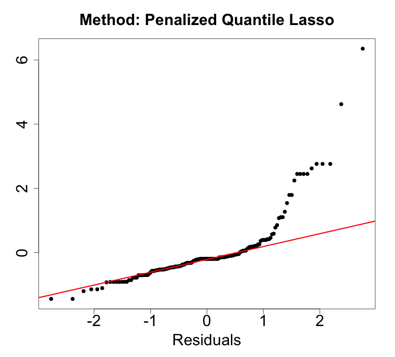
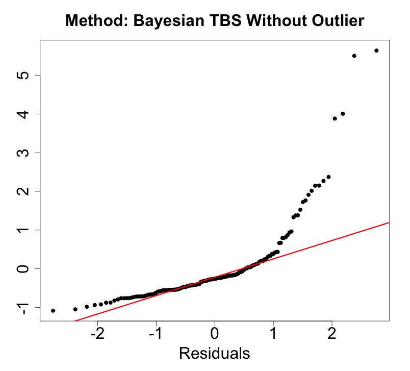
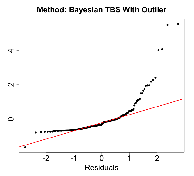
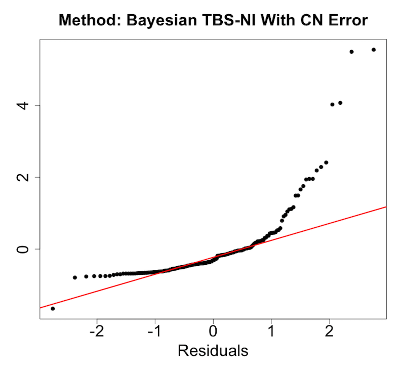
Figure 2: Q-Q plots of observed residuals obtained from 4 methods

From Q-Q plots in Figure 2, it is obvious that the normality assumption about un-transformed response is untenable. We now compare the goodness-of-fit of the three Bayesian methods to evaluate their abilities from handling skewness and heteroscedasticity. For this purpose, we use the residual $g_{\hat{\eta}}(y_{i0})-g_{\hat{\eta}}(x_{i}^{T}\hat{\beta})$ for the Bayesian TBS-SG model of (1) and the TBSCN-SG model of (9), and the residual $g_{\hat{\eta}}(y_{i0})-g_{\hat{\eta}}(x_{i}^{T}\hat{\beta})-\hat{\gamma_{i}}$ for Bayesian TBSO-SG model of (8), and then display their Q-Q plots in Figure 3. It is evident from the Q-Q plots that TBSO-SG model of (8) has the best justification to use it for Bayesian analysis, and TBSCN-SG model of (9) also performs well except may be for some observations in both tails.

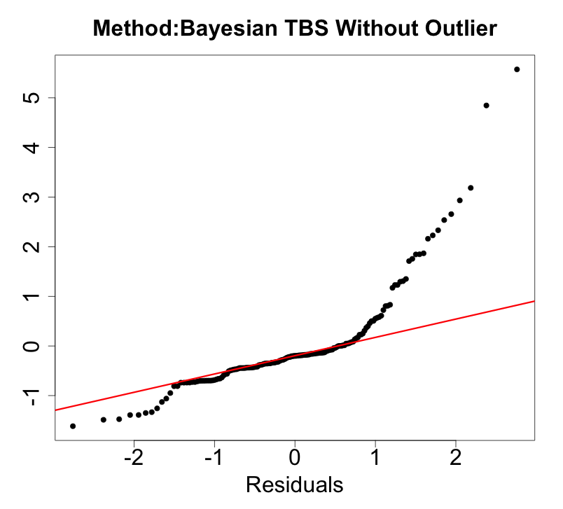
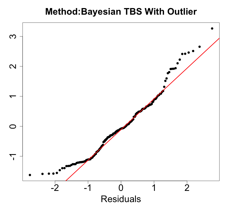
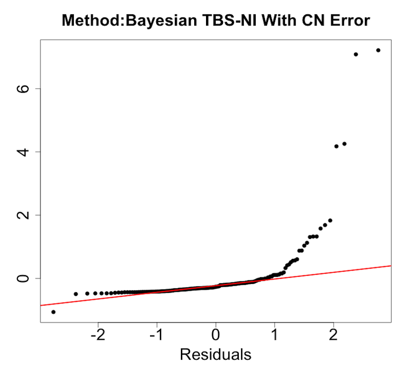
Figure 3: Q-Q plots for residuals of transformed responses obtained from 3 Bayesian models

Using our Bayesian model of (8), we find large posterior evidence of effects of OVERCOME variable with posterior mean=$-0\mbox{$\cdot$}17$ and $95\%$ credible interval ($-0\mbox{$\cdot$}21,-0\mbox{$\cdot$}12$), stroke with posterior mean=$0\mbox{$\cdot$}92$ and $95\%$ credible interval ($0\mbox{$\cdot$}66,1\mbox{$\cdot$}23$), and medication with posterior mean=$-0\mbox{$\cdot$}35$ and $95\%$ credible interval ($-0\mbox{$\cdot$}41,-0\mbox{$\cdot$}24$). Model(9) identifies these same predictors of model (8) with slightly different interval estimates. Model (1) also identifies three predictors with large posterior evidence of effects: perceived health status, stroke and the indicator of major ethnic group. Stroke is the only variable with large posterior evidence of effects in all three models. Even though penalized quantile regression based analysis selects a larger number of predictors compared to the number of predictors selected by our models, the only statistically significant variable from quantile regression analysis is age (estimate of $0\mbox{$\cdot$}08$ with standard error $0\mbox{$\cdot$}03$). This may be explained by the larger estimated standard errors of the estimates from quantile regression compared to the posterior standard deviations of the corresponding parameters obtained via Bayesian analysis.

In order to better understand the prediction performance on observed data, we present a scatter plot with overlaid quantile lines for each Bayesian method in Figure 4. For each method, we display scaled $x_{i}^{T}\hat{\beta}$ and scaled observed response $y_{i0}$, along with estimated 25th percentile and 75th percentile curves using $g_{\hat{\eta}}^{-1}\{g_{\hat{\eta}}(x_{i}^{T}\beta)+Z_{\alpha}^{*}\}$, where $Z_{\alpha}^{*}$ is estimated $\alpha$-percentile of $f_{e}(\cdot)$. Figure 4 shows that the method using (8) explains the observed data better than methods using (1) and (9). The observations with large errors identified by analysis using (8) are marked by asterisk signs in the second plot. We find that all the observations identified by (8) are outside the estimated interquartile ranges. It shows that our transform-both-sides model of (8) is successful in handling data with skewness, heteroscadesticity as well as very large errors in few subjects. Model of (9) is also able to handle skewness and heteroscadesticity but is not able to identify observations with extremely large errors.

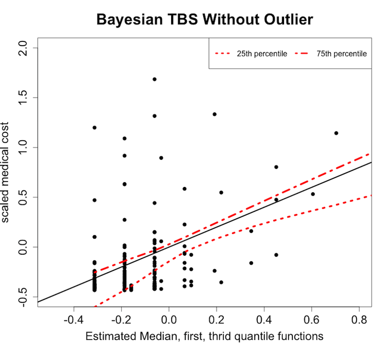
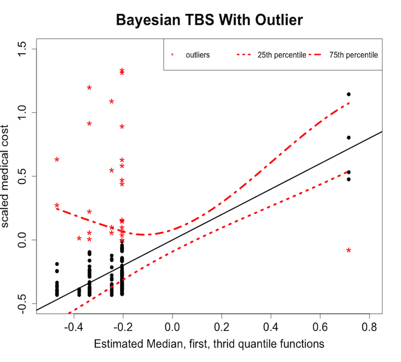
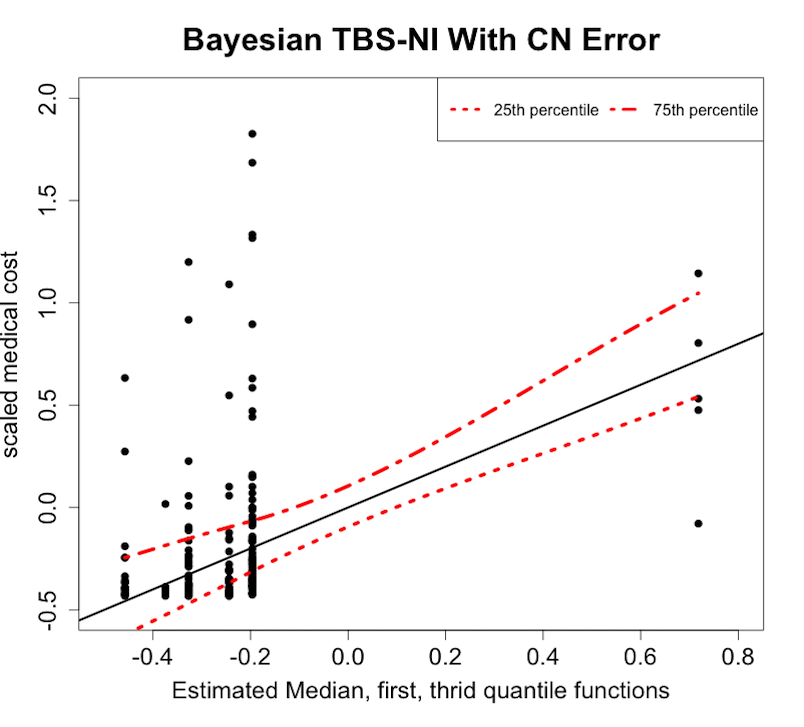
Figure 4: Scatter plots of scaled observed responses and quantile regression functions obtained from 3 Bayesian models

We also use posterior predictive loss approach (Gelfand and Ghosh, 1998) to evaluate the prediction accuracy under each Bayesian method. We compute the prediction errors of our Bayesian methods by $\sum_{i=1}^{n}\mbox{E}[\{g_{\hat{\eta}}(y_{i0})-g_{\hat{\eta}}(x_{i}^{T}\hat{\beta})\}^{2}|D]$ from model (1), and by $\sum_{i=1}^{n}E[\{g_{\hat{\eta}}(y_{i0})-g_{\hat{\eta}}(x_{i}^{T}\hat{\beta})-\gamma_{i}\}^{2}|D]$ for model (8) using MCMC approximation, where $D$ is the observed dataset. The average prediction error from model (8) is $15\cdot 03$, which is considerably better than model (1) with average prediction error $174\cdot 45$.

7 Discussion

In this article, we propose Bayesian variable selection methods for skewed and heteroscedastic response. The methods are highly suitable for modeling, computation, analysis and interpretation of real-life health care cost studies, where we aim to determine and estimate effects of a sparse set of explanatory variables for health care expenditures out of a large set of potential explanatory variables. Simulation results indicate a better performance of our Bayesian methods compared to existing frequentist quantile regression tools. Also, our Bayesian approaches provide flexible and robust estimations to incorporate a wide variety of practical situations. The advantages of our Bayesian methods include their practical and easy implementation using standard statistical software. In the appendix, we prove the consistency of variable selection even when the number of potential predictors $p$ is comparable to, however, smaller than $n$. The proofs are only provided for a special case of the covariate matrix and when the transform parameter $\eta$ is known. Proof for a more general case can be obtained following a similar, but more tedious mathematical arguments.

Proof of Theorem 1

For $\gamma\in\{0,1\}^{p}$ and $x\in\mathbb{R}^{p}$, define $x_{\gamma}\in\mathbb{R}^{p_{\gamma}}$ to be the vector $(x_{j}:\gamma_{j}\neq 0)$. The log-likelihood corresponding to (1) has the expression

$$\ell(\beta)=\sum_{i=1}^{n}\log\big{(}g_{\eta}^{\prime}(y_{i})\big{)}-\frac{n}{2}\log(2\pi)-n\log(\sigma)-\frac{1}{2\sigma^{2}}\left\|g_{\eta}(y)-g_{\eta}(X\beta)\right\|^{2},$$ (11)

where $g_{\eta}(y)=\big{(}g_{\eta}(y_{1}),\cdots,g_{\eta}(y_{n})\big{)}^{\mathrm{\scriptscriptstyle T}}$, $g_{\eta}(X\beta)=\big{\{}g_{\eta}(x_{1}^{\mathrm{\scriptscriptstyle T}}\beta),\cdots,g_{\eta}(x_{n}^{\mathrm{\scriptscriptstyle T}}\beta)\big{\}}^{\mathrm{\scriptscriptstyle T}}$. The gradient of (11) is given by

$$\nabla\ell(\beta)=\frac{1}{\sigma^{2}}X^{\mathrm{\scriptscriptstyle T}}\bar{D}_{\eta}\big{(}g_{\eta}(y)-g_{\eta}(X\beta)\big{)},$$ (12)

where $\bar{d}_{\eta}=(g_{\eta}^{\prime}(x_{1}^{T}\beta),\cdots,g_{\eta}^{\prime}(x_{n}^{T}\beta))$ with $g_{\eta}^{\prime}(x_{i}^{T}\beta)=\left\lvert x_{i}^{T}\beta\right\rvert^{\eta-1}$ and $\bar{D}_{\eta}=\text{diag}(\bar{d}_{\eta})$. $\beta\mapsto\nabla\ell(\beta)$ is continuous. Since the number of true signals $\beta_{j}^{*}$ is finite, we assume $\beta_{j}^{*}\in[M_{L},M_{U}]$. Hence, as long as $\beta$ is in a neighborhood of $\beta^{*}$, $\nabla\ell(\beta)$ is bounded since $\left\lvert x_{i}^{T}\beta\right\rvert^{\eta-1}$ in (12) is bounded when $\eta\in(1,2)$. The Hessian of (11) is defined as

$$H(\beta)=\frac{1}{\sigma^{2}}X^{T}\big{(}-\bar{D}_{\eta}^{T}\bar{D}_{\eta}+\bar{\bar{D}}_{\eta}^{T}M_{\beta}(y,X)\big{)}X,$$ (13)

where $\bar{\bar{d}}_{\eta}$ is defined as the element-wise second derivative of $g_{\eta}(x_{i}^{T}\beta)$ on $\beta$ with $g_{\eta}^{\prime\prime}(x_{i}^{T}\beta)=\text{\mbox{sgn}}(x_{i}^{T}\beta)(\eta-1)\left\lvert x_{i}^{T}\beta\right\rvert^{\eta-2}$ and $\bar{\bar{D}}_{\eta}=\text{diag}(\bar{\bar{d}}_{\eta})$. Meanwhile, $m_{\eta}(y,X)=\big{(}g_{\eta}(y_{1})-g_{\eta}(x_{1}^{T}\beta),\cdots,g_{\eta}(y_{n})-g_{\eta}(x_{n}^{T}\beta)\big{)}$ and $M_{\eta}(y,X)=\text{diag}(m_{\eta}(y,X))$. Using Laplace approximation, the Bayes factor can be approximated as

$$\frac{p(y|\beta,\gamma)}{p(y|\beta^{*},\gamma^{*})}=(2\pi)^{\frac{p_{\gamma}-p_{\gamma^{*}}}{2}}\times e^{\{\ell(\tilde{\beta}_{\gamma})-\ell(\beta^{*}_{\gamma^{*}})\}}\times\frac{\pi(\tilde{\beta}_{\gamma}|\gamma)}{\pi(\beta^{*}_{\gamma^{*}}|\gamma^{*})}\times\frac{|H(\beta^{*}_{\gamma^{*}}|\gamma^{*})|^{1/2}}{|H(\tilde{\beta}_{\gamma}|\gamma)|^{1/2}}.$$ (14)

The first term in the r.h.s of (14) is $\big{(}O_{p}(1)\big{)}^{n}$ with $p\leq n$. For the second term, we denote by $\lambda(y)=\ell(\tilde{\beta})-\ell(\beta^{*})$ the likelihood ratio statistic. As in Rossell and Telesca (2015, Proposition 3), it is straightforward to verify that our sampling model (1) satisfies Walker’s conditions (A1)-(A5) and (B1)-(B4) (Walker, 1969). Hence, our MLE $\tilde{\beta_{i}}$ is consistent and the Hessian matrix $H(\tilde{\beta}_{\gamma}|\gamma)$ in (14) converges in probability. We consider two cases below.

When $\gamma^{*}\not\subset\gamma$, i.e., $\gamma$ misses some true active coefficients, the second term $e^{(\text{log}L(\tilde{\beta}_{\gamma})-\text{log}L(\beta^{*}_{\gamma^{*}}))}\xrightarrow{P}e^{-n\text{KL}(p(y|\beta^{*},\gamma^{*}),p(y|\beta,\gamma))}$ where $\text{KL}(p(y|\beta^{*},\gamma^{*}),p(y|\beta,\gamma))$ is the Kullback-Leibler divergence between optimal $p(y|\beta^{*},\gamma^{*})$ and $p(y|\beta,\gamma)$ under $\gamma$. Here the minimum KL divergence $\text{KL}(p(y|\beta^{*},\gamma^{*}),p(y|\beta,\gamma))$ is strictly positive since,

$$\text{KL}(p(y|\beta^{*},\gamma^{*}),p(y|\beta,\gamma)) = \sum_{i=1}^{n}\int[\text{log}(p(y_{i}|\beta^{*},\gamma^{*}))-\text{log}(p(y_{i}|\beta,\gamma))]p(y_{i}|\beta^{*},\gamma^{*})d_{y_{i}}$$ (15)

$$= \frac{1}{2\sigma^{2}}\sum_{i=1}^{n}\Big{(}E\big{(}g_{\eta}(y_{i})-g_{\eta}(x_{i}^{T}\beta)\big{)}^{2}-E\big{(}g_{\eta}(y_{i})-g_{\eta}(x_{i}^{T}\beta^{*})\big{)}^{2}\Big{)}$$

$$= \frac{1}{2\sigma^{2}}\sum_{i=1}^{n}\big{(}g_{\eta}(x_{i}^{T}\beta^{*})-g_{\eta}(x_{i}^{T}\beta)\big{)}^{2}>0$$

when $\beta\neq\beta^{*}$ satisfies the eigenvalue conditions in §3 that indicates no linear dependency among covariates $x_{i}$. Therefore the second term is $O_{p}(e^{-n})$ when $\gamma^{*}\not\subset\gamma$.

When $\gamma^{*}\subset\gamma$, we denote the likelihood-ratio statistic by $\Lambda(y)=\text{log}L(\tilde{\beta}_{\gamma})-\text{log}L(\beta^{*}_{\gamma^{*}})$. Under appropriate regularity conditions (Hogg et al., 2013), our likelihood ratio statistic $\Lambda(y)$ is asymptotically chi-square distributed. The regularity conditions relevant to the argument are listed as (R0)-(R9) in Hogg et al. (2013) where (R0)-(R2) and (R6)-(R8) can be obtained trivially. Conditions (R3) and (R4) are related to Fisher information and are satisfied by Hessian matrix (13). Conditions (R5) and (R9) essentially guarantee that the remainder of a second order Taylor expansion around $\beta$ is bounded in probability. To that end, note that

$$\left|\frac{\partial^{3}}{\partial\beta_{j}\partial\beta_{k}\partial\beta_{l}}\ell(\beta)\right|$$ (16)

$$= \left|\frac{\eta-1}{\sigma^{2}}\sum_{i=1}^{n}x_{ij}x_{ik}x_{il}\Big{[}-\big{(}2+\mbox{sgn}(x_{i}^{T}\beta)\big{)}|x_{i}^{T}\beta|^{2\eta-3}+(\eta-2)\big{(}g_{\eta}(y_{i})-g_{\eta}(x_{i}^{T}\beta)\big{)}|x_{i}^{T}\beta|^{\eta-3}\Big{]}\right|$$

$$\leq \frac{\eta-1}{\sigma^{2}}\sum_{i=1}^{n}x_{ij}x_{ik}x_{il}\Big{[}3|x_{i}^{T}\beta|^{2\eta-3}+\mid g_{\eta}(y_{i})-g_{\eta}(x_{i}^{T}\beta)\mid|x_{i}^{T}\beta|^{\eta-3}\Big{]}:=M_{jkl}(y;X)$$

where $E[M_{jkl}(y;x)]<\infty$ for all $j,k,l\in 1,\cdots,p$. Therefore our model (1) satisfies all regularity conditions implying $\Lambda(y)\sim\chi_{p_{\gamma}-p_{\gamma^{*}}}^{2}$ and hence $O_{p}(1)$ as required. When $\gamma$ has moderate size with $p_{\gamma}\leq n$, we will show the first term in (14) is dominated by the second term later.

Next consider the second term $\pi(\tilde{\beta}|\gamma)/\pi(\beta^{*}|\gamma^{*})$ under a non-local prior with $\eta\in(1,2)$ is known.

$$\frac{\pi(\tilde{\beta}|\gamma)}{\pi(\beta^{*}|\gamma^{*})} = \frac{\prod_{i=1}^{p_{\gamma}}\frac{1}{\sqrt{2\pi}\sigma_{\beta}}\text{exp}(-\tilde{\beta}_{\gamma_{i}}^{2}/2\sigma_{\beta}^{2})|\tilde{\beta}_{\gamma_{i}}|^{\eta-1}}{\prod_{j=1}^{p_{\gamma^{*}}}\frac{1}{\sqrt{2\pi}\sigma_{\beta}}\text{exp}(-\beta^{*2}_{\gamma^{*}_{j}}/2\sigma_{\beta}^{2})|\beta^{*}_{\gamma^{*}_{j}}|^{\eta-1}}$$ (17)

$$= (\frac{1}{\sqrt{2\pi}\sigma_{\beta}})^{p_{\gamma}-p_{\gamma^{*}}}\text{exp}\big{(}-(\sum\tilde{\beta}_{\gamma_{i}}^{2}-\sum\beta^{*2}_{\gamma^{*}_{j}})/2\sigma_{\beta}^{2}\big{)}\frac{\prod|\tilde{\beta}_{\gamma_{i}}|^{\eta-1}}{\prod|\beta^{*}_{\gamma^{*}_{j}}|^{\eta-1}}$$

First if $\gamma^{*}\subset\gamma$, given that $\tilde{\beta}_{\gamma_{i}}=O_{p}(n^{-1/2})$ and $\eta-1>0$, the second term is ensentially $O_{p}(n^{-(\eta-1)(p_{\gamma}-p_{\gamma^{*}})/2})$. When $\gamma^{*}\not\subset\gamma$, denote $s^{*}=\gamma\cap\gamma^{*}$, the second term is $O_{p}(n^{-(\eta-1)(p_{\gamma}-p_{s^{*}})/2})$ and upper bounded by $O_{p}(n^{-(\eta-1)/2})$.

To conclude the proof, we need to deal with the the third term in (14). The Hessian matrix $H(\tilde{\beta})$ is given by (13) with each element $H_{ij}=X_{i}^{T}X_{j}O_{p}(1)$. Since $\tilde{\beta_{\gamma}}$ converge in probability to $\beta_{\gamma^{*}}$, we have $n^{-1}H(\tilde{\beta}|\gamma)\xrightarrow{p}H(\tilde{\beta}|\gamma)$. Therefore by continous mapping theorem, the third term in (14) is approximated as

$$\frac{\left\lvert H(\beta^{*}|\gamma^{*})\right\rvert^{1/2}}{\left\lvert H(\tilde{\beta}|\gamma)\right\rvert^{1/2}}\asymp\frac{n^{p_{\gamma^{*}/2}}}{n^{p_{\gamma}/2}}\frac{\left\lvert n^{-1}H(\beta_{0}|\gamma^{*})\right\rvert}{\left\lvert n^{-1}H(\tilde{\beta}|\gamma)\right\rvert}=O_{p}(n^{(p_{\gamma^{*}}-p_{\gamma})/2}).$$ (18)

To conclude, the Bayes factor (14) is $O_{p}(n^{-\eta(p_{\gamma}-p_{\gamma^{*}})/2})$ when $\gamma^{*}\subset\gamma$, and $O_{p}(n^{(p_{\gamma^{*}}-p_{\gamma})/2}e^{-n})$ when $\gamma^{*}\not\subset\gamma$. Then the posterior probability $p(\gamma=\gamma^{*}\mid y)$ can be lower-bounded as

$$p(\gamma=\gamma^{*}\mid y) = \frac{p(y\mid\gamma^{*})\pi(\gamma^{*})}{p(y\mid\gamma^{*})\pi(\gamma^{*})+\sum_{\gamma\neq\gamma^{*}}p(y\mid\gamma)\pi(\gamma)}$$

$$= \Big{[}1+\sum_{\gamma^{*}\subset\gamma}\frac{p(y\mid\gamma)\pi(\gamma)}{p(y\mid\gamma^{*})\pi(\gamma^{*})}+\sum_{\gamma^{*}\not\subset\gamma}\frac{p(y\mid\gamma)\pi(\gamma)}{p(y\mid\gamma^{*})\pi(\gamma^{*})}\Big{]}^{-1}$$

$$\geq \Big{[}1+\sum_{\gamma^{*}\subset\gamma}O_{p}(n^{-\eta(p_{\gamma}-p_{\gamma^{*}})/2})+\sum_{\gamma^{*}\not\subset\gamma}O_{p}(n^{(p_{\gamma^{*}}-p_{\gamma})/2}e^{-n})\Big{]}^{-1}$$

$$\geq \Big{[}1+\sum_{\gamma^{*}\subset\gamma}O_{p}(n^{-(p_{\gamma}-p_{\gamma^{*}})/2})+\sum_{\gamma^{*}\not\subset\gamma}O_{p}(e^{-n})\Big{]}^{-1}\xrightarrow{a.s.}1$$

which concludes the proof.

References

- (1)
- Bach (2008) Bach, F. R. (2008), Bolasso: model consistent lasso estimation through the bootstrap, in ‘Proceedings of the 25th International Conference on Machine learning’, ACM, pp. 33–40.
- Bhattacharya et al. (2014) Bhattacharya, A., Pati, D., Pillai, N. and Dunson, D. (2014), ‘Dirichlet-laplace priors for optimal shrinkage’, JASA .
- Bickel and Doksum (1981) Bickel, P. J. and Doksum, K. A. (1981), ‘An analysis of transformations revisited’, JASA 76(374), 296–311.
- Bondell and Reich (2012) Bondell, H. D. and Reich, B. J. (2012), ‘Consistent high-dimensional bayesian variable selection via penalized credible regions’, JASA 107(500), 1610–1624.
- Carvalho et al. (2010) Carvalho, C., Polson, N. and Scott, J. (2010), ‘The horseshoe estimator for sparse signals’, Biometrika 97(2), 465–480.
- Castillo et al. (2014) Castillo, I., Schmidt-Hieber, J. and van der Vaart, A. W. (2014), ‘Bayesian linear regression with sparse priors’, ArXiv e-prints .
- Chen et al. (2014) Chen, L., Pourahmadi, M. and Maadooliat, M. (2014), ‘Regularized multivariate regression models with skew-t error distributions’, Journal of Statistical Planning and Inference 149, 125 – 139.
- Cohen (2003) Cohen, S. B. (2003), ‘Design strategies and innovations in the medical expenditure panel survey’, Medical Care 41(7), III.
- Efron et al. (2004) Efron, B., Hastie, T., Johnstone, I. and Tibshirani, R. (2004), ‘Least angle regression’, The Annals of statistics 32(2), 407–499.
- Fan and Li (2001) Fan, J. and Li, R. (2001), ‘Variable selection via nonconcave penalized likelihood and its oracle properties’, JASA 96(456), 1348–1360.
- Gelfand and Ghosh (1998) Gelfand, A. E. and Ghosh, S. K. (1998), ‘Model choice: A minimum posterior predictive loss approach’, Biometrika 85(1), 1–11.
- George and McCulloch (1997) George, E. I. and McCulloch, R. E. (1997), ‘Approaches for Bayesian variable selection’, Statistica Sinica 7(2), 339–373.
- George and McCulloch (1993) George, E. and McCulloch, R. (1993), ‘Variable selection via Gibbs sampling’, JASA 88(423), 881–889.
- Hampel et al. (2011) Hampel, F. R., Ronchetti, E. M., Rousseeuw, P. J. and Stahel, W. A. (2011), Robust Statistics: the Approach Based on Influence Functions, Vol. 114, Wiley.
- Hogg et al. (2013) Hogg, R., McKean, J. and Craig, A. (2013), Introduction to Mathematical Statistics, Pearson.