A globally convergent numerical method for a 1-d inverse medium problem with experimental data

Abstract

In this paper, a reconstruction method for the spatially distributed dielectric constant of a medium from the back scattering wave field in the frequency domain is considered. Our approach is to propose a globally convergent algorithm, which does not require any knowledge of a small neighborhood of the solution of the inverse problem in advance. The Quasi-Reversibility Method (QRM) is used in the algorithm. The convergence of the QRM is proved via a Carleman estimate. The method is tested on both computationally simulated and experimental data.

2010 Mathematics Subject Classification: 34L25, 35P25, 35R30, 78A46.

Keywords: coefficient inverse scattering problem, globally convergent algorithm, dielectric constant, electromagnetic waves.

1 Introduction

In this paper we develop a globally convergent numerical method for a 1-d inverse medium problem in the frequency domain. The performance of this method is tested on both computationally simulated and experimental data. Propagation of electromagnetic waves is used in experiments. A theorem about the global convergence of our method is proved. Another name for inverse medium problems is Coefficient Inverse Problems (CIPs). We model the process as a 1-d CIP due to some specifics of our data collection procedure, see subsection 6.2. This paper is the first one in which the globally convergent method of [1, 2, 11, 18, 19, 28, 29] is extended to the case of the frequency domain. Indeed, the original version of that method works with the Laplace transform of the time dependent data. Both the 3-d and the 1-d versions of the method of [1, 2] were verified on experimental data, see [1, 28, 29] for the 3-d case and [11, 18, 19] for the 1-d case. The experimental data here are the same ones as in [11, 18, 19].

Compared with the previous publications [11, 18, 19], two additional difficulties occurring here are: (1) we now work with complex valued functions instead of real valued ones and, therefore (2) it is not immediately clear how to deal with the imaginary part of the logarithm of the complex valued solution of the forward problem. On the other hand, we use that logarithm in our numerical procedure. Besides, the previous numerical scheme of [11, 18, 19] is significantly modified here.

We call a numerical method for a CIP globally convergent if there is a rigorous guarantee that this method reaches at least one point in a sufficiently small neighborhood of the correct solution without any advanced knowledge about this neighborhood. It is well known that the topic of the global convergence for CIPs is a highly challenging one. Thus, similarly with the above cited publications, we prove the global convergence of our method within the framework of a certain approximation. This is why the term “approximate global convergence” was used in above cited references (“global convergence” in short). That approximation is used only on the first iterative step of our algorithm and it is not used in follow up iterations. Besides, this approximation is a quite natural one, since it amounts to taking into account only the first term of a certain asymptotic behavior and truncating the rest. The global convergence property is verified numerically here on both computationally simulated and experimental data.

CIPs are both highly nonlinear and ill-posed. These two factors cause the non-convexity of conventional Tikhonov functionals for these problems. It is well known that typically those functionals have multiple local minima and ravines, see, e.g. numerical examples of multiple local minima in [26] and on Figure 5.3 of [14]. Figure 5.4 of [14] demonstrates an example of a ravine. Hence, there is no guarantee of the convergence of an optimization method to the correct solution, unless the starting point of iterations is located in a sufficiently small neighborhood of that solution. However, it is often unclear in practical scenarios how to reach that neighborhood.

In our inverse algorithm we solve a sequence of linear ordinary differential equations of the second order on the interval $x\in\left(0,1\right)$. The peculiarity here is that we have overdetermined boundary conditions for these equations: we have the solution and its first derivative at $x=0$ and we have the first derivative of the solution at $x=1$. Our attempts to use only boundary conditions at $x=0$ did not lead to good reconstruction results. The same observation is in place in Remark 5.1 on page 13 of [18]. Thus, similarly with [11, 18, 19], we use here the Quasi-Reversibility Method (QRM). The QRM is well suitable to solve PDEs with the overdetermined boundary data. To analyze the convergence rate of the QRM, we use a Carleman estimate.

The QRM was first introduced by Lattes and Lions [20]. However, they have not established convergence rates. These rates were first established in [12, 13], where it was shown that Carleman estimates are the key tool for that goal. A survey of applications of Carleman estimates to QRM can be found in [16]. Chapter 6 of [1] describes the use of the QRM for numerical solutions of CIPs. We also mention an active work with the QRM of Bourgeois and Dardè, see, e.g. [4, 5, 6] for some samples of their publications.

Our experimental data are given in the time domain. To obtain the data in the frequency domain, we apply the Fourier transform. Previously the same data were treated in works [11, 18, 19] of this group. In that case the Laplace transform was applied. Next, the 1-d version of the globally convergent method of [1, 2] was used. Indeed, the original version of this method works with the Laplace transform of the time dependent data. A similar 1-d inverse problem in the frequency domain was solved numerically in [21] by a different method.

The experimental data of this publication were collected by the Forward Looking Radar which was built in the US Army Research Laboratory [23]. The data were collected in the field (as opposed to a laboratory). Thus, clutter was present at the measurement site. This certainly adds some additional difficulties to the imaging problem. The goal of this radar is to detect and identify shallow explosives, such as, e.g. improvised explosive devices and antipersonnel land mines. Those explosives can be located either on the ground surface or a few centimeters below this surface. This radar provides only a single time dependent curve for a target. Therefore, to solve a CIP, we have no choice but to model the 3-d process by a 1-d wave-like PDE. We model targets as inclusions whose dielectric constants are different from the background.

In terms of working with experimental data, the goal in this paper is not to image locations of targets, since this is impossible via solving a CIP with our data, see subsection 6.2 for details. In fact, our goal is to image maximal values of dielectric constants of targets. Our targets are 3-d objects, while we use a 1-d model: since we measure only one time resolved curve for a target. Nevertheless, we show below that our calculated dielectric constants are well within tabulated limits [27].

Of course, an estimate of the dielectric constant is insufficient for the discrimination of explosives from the clutter. On the other hand, the radar community mostly relies on the intensity of the radar image. Therefore, we hope that the additional information about values of dielectric constants of targets might lead in the future to designs of algorithms which would better discriminate between explosives and clutter.

In the 3-d case the globally convergent method of [1, 2, 28, 29] works with the data generated either by a single location of the source or by a single direction of the incident plane wave. The second globally convergent method for this type of measurements was developed and tested numerically in [15]. We also refer to another globally convergent methods for a CIPs, which is based on the multidimensional version of the Gelfand-Levitan method. This version was first developed by Kabanikhin [8] and later by Kabanikhin and Shishlenin [9, 10]. Unlike [1, 2, 28, 29], the technique of [8, 9, 10] works with multiple directions of incident plane waves.

In [11] the performance of the method of [18, 19] was compared numerically with the performance of the Krein equation [17] for the same experimental data as ones used here. The Krein equation [17] is close to the Gelfand-Levitan equation [22]. It was shown in [17] that the performance of the Krein equation is inferior to the performance of the method of [18, 19] for these experimental data. This is because the solution of the Krein equation is much more sensitive to the choice of the calibration factor than the solution obtained by the technique of [18, 19]. On the other hand, it is necessary to apply that factor to those experimental data to make the range of values of the resulting data comparable with the range of values of computationally simulated data.

In section 2 we pose forward and inverse problems and analyze some of their features. In section 3 we study a 1-d version of the QRM. In section 4 we present our globally convergent method. In section 5 we prove the global convergence of our method. In section 6 we present our numerical results for both computationally simulated and experimental data.

2 Some Properties of Forward and Inverse Problems

It was shown numerically in [3] that the component of the electric field, which is incident upon a medium, dominates two other components. It was also shown in [3] that the propagation of that component is well governed by a wave-like PDE. Furthermore, this finding was confirmed by imaging from experimental data, see Chapter 5 of [1] and [28, 29]. Thus, just as in [11, 18, 19], we use a 1-d wave-like PDE to model the collection of our experimental data of electromagnetic waves propagation.

2.1 Formulations of problems

Let $c_{0}<c_{1}$ be two positive numbers. Let the function $c:\mathbb{R}\rightarrow\mathbb{R}$ satisfy the following conditions:

$$c \in C^{2}\left(\mathbb{R}\right),c\left(x\right)\in\left[c_{0},c_{1}\right],\forall x\in\mathbb{R},$$ (2.1)

$$c\left(x\right) = 1+\beta\left(x\right),\beta\left(x\right)=0,\forall x\notin\left(0,1\right).$$ (2.2)

Fix the source position $x_{0}<0$. Consider the generalized Helmholtz equation in the 1-d case,

$$u^{\prime\prime}+k^{2}c\left(x\right)u = -\delta\left(x-x_{0}\right),x\in\mathbb{R},$$ (2.3)

$$\lim_{x\rightarrow\infty}\left(u^{\prime}+iku\right) = 0,\lim_{x\rightarrow-\infty}\left(u^{\prime}-iku\right)=0.$$ (2.4)

Let $u_{0}\left(x,x_{0},k\right)$ be the solution of the problem (2.3), (2.4) for the case $c\left(x\right)\equiv 1.$ Then

$$u_{0}\left(x,x_{0},k\right)=\frac{\exp\left(-ik\left|x-x_{0}\right|\right)}{2ik}.$$ (2.5)

The problem (2.3), (2.4) is the forward problem. Our interest is in the following inverse problem problem:

Problem (Coefficient Inverse Problem (CIP)).

Fix the source position $x_{0}<0.$ Let $[\underline{k},\overline{k}]\subset\left(0,\infty\right)$ be an interval of frequencies $k$. Reconstruct the function $\beta\left(x\right),$ assuming that the following function $g_{0}\left(k\right)$ is known

$$g_{0}\left(k\right)=\frac{u(0,x_{0},k)}{u_{0}(0,x_{0},k)},k\in[\underline{k},\overline{k}].$$ (2.6)

2.2 Some properties of the solution of the forward problem

In this subsection we establish existence and uniqueness of the forward problem. Even though these results are likely known, we present them here for reader’s convenience. In addition, the techniques using in their proofs help us to verify that the function $u(x,x_{0},k)$ never vanishes for $x>x_{0}$, which plays an important role in our algorithm of solving the to CIP. Also, this technique justifies the numerical method for solving the forward problem (2.3), (2.4). Computationally simulated data are obtained by numerically solving the problem (2.3), (2.4).

Theorem 2.1.

Assume that conditions (2.1)-(2.2) hold. Then for each $k>0$ and for each $x_{0}<0$ there exists a single solution $u\left(x,x_{0},k\right)$ of the problem (2.3), (2.4). Moreover, the function $\widetilde{u}\left(x,x_{0},k\right)=u\left(x,x_{0},k\right)-u_{0}\left(x,x_{0},k\right)$, called the scattering field, is in $C^{3}\left(\mathbb{R}\right)$.

Proof. We prove uniqueness first. Suppose that ${u}_{1}$ and ${u}_{2}$ are two solutions of the problem (2.3), (2.4). Denote $U=u_{1}-u_{2}.$ Then the function $U$ satisfies

$$U^{\prime\prime}+k^{2}\left(1+\beta\left(x\right)\right)U = 0,x\in\mathbb{R},$$ (2.7)

$$\lim_{x\rightarrow\infty}\left(U^{\prime}+ikU\right) = 0,\lim_{x\rightarrow-\infty}\left(U^{\prime}-ikU\right)=0.$$ (2.8)

Since the function $\beta\left(x\right)=0$ outside of the interval $\left(0,1\right),$ then (2.7) implies that $U^{\prime\prime}+k^{2}U=0$ for $x\notin\left(0,1\right).$ This, together with (2.8), yields

$$U\left(x,x_{0},k\right)=\left\{\begin{array}[]{c}B_{1}\left(x_{0},k\right)e^{-ikx},x>1,\\ B_{2}\left(x_{0},k\right)e^{ikx},x<0,\end{array}\right.$$ (2.9)

where $B_{1}$ and $B_{2}$ are some complex numbers depending on $x_{0},k.$

Let $R>1$ be an arbitrary number. Multiply both sides of (2.7) by the function $\overline{U}$ and integrate over the interval $\left(-R,R\right)$ using integration by parts. We obtain

$$\left(U^{\prime}\overline{U}\right)\left(R\right)-\left(U^{\prime}\overline{U}\right)\left(-R\right)-\mathop{\displaystyle\int}\limits_{-R}^{R}\left|U^{\prime}\right|^{2}dx+k^{2}\mathop{\displaystyle\int}\limits_{-R}^{R}\left(1+\beta\left(x\right)\right)\left|U\right|^{2}dx=0.$$ (2.10)

By (2.9) $\left(U^{\prime}\overline{U}\right)\left(R\right)=-ik\left|B_{1}\right|^{2}$ and $-\left(U^{\prime}\overline{U}\right)\left(-R\right)=-ik\left|B_{2}\right|^{2}.$ Hence, the imaginary part of (2.10), $-k\left(\left|B_{1}(x_{0},k)\right|^{2}+\left|B_{2}(x_{0},k)\right|^{2}\right)=0,$ vanishes, so do $B_{1}(x_{0},k)$ and $B_{2}(x_{0},k)$. Using (2.9), we obtain $U\left(x,x_{0},k\right)=0$ for $x\notin\left(0,1\right).$ Due to the classical unique continuation principle, $U\left(x,x_{0},k\right)=0,\forall x\in\mathbb{R}.$ Thus, $u_{1}=u_{2}$.

We now prove existence. Consider the 1-d analog of the Lippman-Schwinger equation with respect to a function $P$,

$$P\left(x,x_{0},k\right)=\frac{\exp\left(-ik\left|x-x_{0}\right|\right)}{2ik}+\frac{k}{2i}\mathop{\displaystyle\int}\limits_{0}^{1}\exp\left(-ik\left|x-\xi\right|\right)\beta\left(\xi\right)P\left(\xi,x_{0},k\right)d\xi,x\in\mathbb{R}.$$ (2.11)

Fix $x_{0}<0$ and $k>0$. Consider equation (2.11) only for $x\in\left(0,1\right).$ Assume that there exist two functions $P_{1},P_{2}$ satisfying (2.11) for $x\in\left(0,1\right).$ Consider their extensions on the set $\mathbb{R}\diagdown\left(0,1\right)$ via the right hand side of (2.11). Then so defined functions $P_{1},P_{2}$ satisfy (2.11) for all $x\in$ $\mathbb{R}.$ Hence, both of them are solutions of the problem (2.3), (2.4). Hence, the above established uniqueness result implies that $P_{1}\equiv P_{2}.$

Consider again the integral equation (2.11) for $x\in\left(0,1\right)$ and apply the Fredholm alternative. This alternative, combined with the discussion in the previous paragraph, implies that there exists unique solution $P\in C\left[0,1\right]$ of equation (2.11). Extending this function for $x\in\mathbb{R}\diagdown\left(0,1\right)$ via the right hand side of (2.11), we obtain that there exists unique solution $P\in C\left(\mathbb{R}\right)$ of equation (2.11). Furthermore, the function $P-u_{0}\in C^{3}\left(\mathbb{R}\right)$ and also this function $P$ is the required solution of the problem (2.3), (2.4). $\square$

Below we consider only such a solution $u$ of the problem (2.3), (2.4) that $u-u_{0}\in C^{3}\left(\mathbb{R}\right)$: as in Theorem 2.1.

2.3 The asymptotic behavior of the function $u(x,x_{0},k)$ as $k\rightarrow\infty$

Consider the function $\phi\left(x\right)$ defined as

$$\phi\left(x\right)=-\frac{c^{\prime\prime}\left(x\right)}{c^{2}\left(x\right)}+\frac{7}{16}\frac{\left(c^{\prime}\left(x\right)\right)^{2}}{c^{3}\left(x\right)}.$$ (2.12)

Note that by (2.2) $\phi\left(x\right)=0$ for $x\notin\left[0,1\right].$

Theorem 2.2.

Assume that the function $\phi\left(x\right)\leq 0,\forall x\in\left[0,1\right].$ Then for every pair $(x,x_{0})\in\mathbb{R}\times(-\infty,0)$, the asymptotic behavior of the function $u\left(x,x_{0},k\right)$ is

$$u\left(x,x_{0},k\right)=\frac{1}{2ikc^{1/4}\left(x\right)}\exp\left[-ik\left|\mathop{\displaystyle\int}\limits_{x_{0}}^{x}\sqrt{c\left(\xi\right)}d\xi\right|\right]\left(1+O\left(\frac{1}{k}\right)\right),k\rightarrow\infty.$$ (2.13)

Furthermore, for any finite interval $\left(a,b\right)\subset\mathbb{R}$ there exists a number $\gamma=\gamma\left(a,b,\phi\right)>0$ such that for all $x\in\left(a,b\right)$ the function $u\left(x,x_{0},k\right)$ can be analytically extended with respect $k$ from $\left\{k:k>0\right\}$ in the half plane $\mathbb{C}_{\gamma}=\left\{z\in\mathbb{C}:\mathop{\mathrm{I}m}z<\gamma\right\}$.

Proof. Consider the following Cauchy problem

$$c\left(x\right)\widehat{u}_{tt} = \widehat{u}_{xx},x\in\mathbb{R},t>0,$$ (2.14)

$$\widehat{u}\left(x,0\right) = 0,\widehat{u}_{t}\left(x,0\right)=\delta\left(x-x_{0}\right).$$ (2.15)

This proof is based on the connection between the solution $u$ of the problem (2.3), (2.4) and the solution $\widehat{u}$ of the problem (2.14), (2.15) via the Fourier transform with respect to $t$. Here and below the Fourier transform is understood in terms of distributions, see, e.g. the book [33] for the Fourier transform of distributions.

We now obtain a hyperbolic equation with potential from equation (2.14). To do this, we use a well known change of variables $x\Leftrightarrow y$ [24]

$$y=\mathop{\displaystyle\int}\limits_{x_{0}}^{x}\sqrt{c\left(\xi\right)}d\xi.$$ (2.16)

Denote $b\left(y\right)=c\left(x\left(y\right)\right).$ By (2.16) $db/dy=c^{\prime}\mid_{x=x\left(y\right)}c^{-1/2}\left(x\left(y\right)\right).$ Hence, (2.14) and (2.15) become

$$\widehat{u}_{tt} = \widehat{u}_{yy}+\frac{b^{\prime}\left(y\right)}{2b\left(y\right)}\widehat{u}_{y},\text{ }y\in\mathbb{R},t>0,$$ (2.17)

$$\widehat{u}\left(y,0\right) = 0,\widehat{u}_{t}\left(y,0\right)=\delta\left(y\right).$$ (2.18)

Consider now a new function $\widehat{v}\left(y,t\right)=\widehat{u}\left(y,t\right)/S\left(y\right),$ where the function $S\left(y\right)=b^{-1/4}\left(y\right)$ is chosen in such a way that the coefficient at $\widehat{v}_{y}$ becomes zero after the substitution $\widehat{u}=S\widehat{v}$ in equation (2.17). Then (2.17) and (2.18) become

$$\widehat{v}_{tt} = \widehat{v}_{yy}+p\left(y\right)\widehat{v},$$ (2.19)

$$\widehat{v}\left(y,0\right) = 0,\widehat{v}_{t}\left(y,0\right)=\delta\left(y\right),$$ (2.20)

$$p\left(y\right) = -\frac{b^{\prime\prime}\left(y\right)}{4b\left(y\right)}+\frac{5}{16}\frac{\left(b^{\prime}\left(y\right)\right)^{2}}{b^{2}\left(y\right)}.$$ (2.21)

It follows from (2.1), (2.2), (2.16) and (2.21) that the function $p\in C\left(\mathbb{R}\right)$ and has a finite support,

$$p\left(y\right)=0\text{ for }y<-x_{0}\text{ and for }y>\mathop{\displaystyle\int}\limits_{x_{0}}^{1}\sqrt{c\left(\xi\right)}d\xi.$$ (2.22)

Recall that $\phi\left(x\right)$ is the function defined in (2.12). Expression (2.21) in the $x-$coordinate becomes

$$p\left(y\left(x\right)\right)=\phi\left(x\right).$$ (2.23)

Let $H\left(z\right),z\in\mathbb{R}$ be the Heaviside function. It is well known that the solution $\widehat{v}\left(y,t\right)$ of the problem (2.19), (2.20) has the following form, see, e.g. Chapter 2 in [24]

$$\widehat{v}\left(y,t,x_{0}\right) = \frac{1}{2}H\left(t-\left|y\right|\right)+\widetilde{v}\left(y,t\right)H\left(t-\left|y\right|\right),$$ (2.24)

$$\widetilde{v}\left(y,t\right) \in C^{2}\left(t\geq\left|y\right|\right),\lim_{t\rightarrow\left|y\right|^{+}}\widetilde{v}\left(y,t\right)=0.$$ (2.25)

The backwards substitution $y\rightarrow x$ transforms the function $p\left(y\right)$ in the function $\phi\left(x\right).$ Hence, (2.23) implies that the function $p\left(y\right)$ in (2.21) is non positive,

$$p\left(y\right)\leq 0,\forall y\in\mathbb{R}.$$ (2.26)

Consider now the operator $\mathcal{F}$ of the Fourier transform,

$$\mathcal{F}\left(f\right)\left(k\right)=\mathop{\displaystyle\int}\limits_{0}^{\infty}f\left(t\right)e^{-ikt}dt,\forall f\in L_{1}\left(0,\infty\right).$$ (2.27)

In the sense of distributions we have

$$\mathcal{F}\left(\frac{1}{2}H\left(t-\left|y\right|\right)\right)=\frac{\exp\left(-ik\left|y\right|\right)}{2ik},k>0,$$ (2.28)

see section 6 in §9 of Chapter 2 of [33]. Consider an arbitrary finite interval $\left(a,b\right)\subset\mathbb{R}.$ Let $s,m\geq 0$ be two arbitrary integers such that $s+m\leq 2$. Since by (2.22) the function $p\left(y\right)$ has a finite support, then (2.26), Lemma 6 of Chapter 10 of the book [32] as well as Remark 3 after that lemma guarantee that functions $\partial_{y}^{s}\partial_{t}^{m}\widetilde{v}\left(y,t\right)$ decay exponentially with respect to $t,$ as long as $y\in\left(a,b\right).$ Hence, one can apply the operator $\mathcal{F}$ to the functions $\partial_{y}^{s}\partial_{t}^{m}\widetilde{v}\left(y,t\right)$ in the regular sense. The assertion about the analytic extension follows from (2.27) and the exponential decay of the functions $\partial_{y}^{s}\partial_{t}^{m}\widetilde{v}\left(y,t\right)$

Let $\widehat{V}\left(y,k,x_{0}\right)=\mathcal{F}\left(\widehat{v}\right).$ The next question is whether the function $\widehat{V}$ satisfies analogs of conditions (2.3), (2.4). Theorem 3.3 of [31] and theorem 6 of Chapter 9 of [32] guarantee that the function $\widehat{V}$  satisfies the following conditions

$$\widehat{V}^{\prime\prime}+k^{2}\widehat{V}+p\left(y\right)\widehat{V} = -\delta\left(y\right),y\in\mathbb{R},$$ (2.29)

$$\lim_{x\rightarrow\infty}\left(\widehat{V}^{\prime}+ik\widehat{V}\right) = 0,\lim_{x\rightarrow-\infty}\left(\widehat{V}^{\prime}-ik\widehat{V}\right)=0.$$ (2.30)

Using (2.25) and the integration by parts, we obtain for $k\rightarrow\infty$

$$\mathcal{F}\left(H\left(t-\left|y\right|\right)\widetilde{v}\right)=\exp\left(-ik\left|y\right|\right)\mathop{\displaystyle\int}\limits_{0}^{\infty}\widetilde{v}\left(y,t+\left|y\right|\right)e^{-ikt}dt=\exp\left(-ik\left|y\right|\right)O\left(\frac{1}{k^{2}}\right).$$ (2.31)

Two backwards substitution: $y\rightarrow x$ via (2.16) and $\widehat{V}\rightarrow u\left(x,x_{0},k\right)=S\left(y\left(x\right)\right)\widehat{V}\left(y\left(x\right),x_{0},k\right)$ imply that conditions (2.29) and (2.30) for the function $\widehat{V}$ turn into conditions (2.3), (2.4) for the function $u$. Thus, (2.28) and (2.31) imply (2.13). $\square$

2.4 Some properties of the solution of the inverse problem

Since the source position $x_{0}<0$ is fixed, we drop everywhere below the dependence on $x_{0}$ in notations of functions. First, we show that, having the function $g_{0}\left(k\right)$ in (2.6), one can uniquely find the function $u_{x}\left(0,k\right).$ Indeed, for $x<0$ conditions (2.3) and (2.4) become

$$u^{\prime\prime}+k^{2}u=-\delta\left(x-x_{0}\right),x\in\left(-\infty,0\right),$$ (2.32)

$$\lim_{x\rightarrow-\infty}\left(u_{x}-iku\right)=0.$$ (2.33)

Let $\widetilde{u}\left(x,k\right)=u-u_{0}.$ Then (2.32) and (2.33) imply that

$$\widetilde{u}^{\prime\prime}+k^{2}\widetilde{u}=0\text{ for }x\in\left(-\infty,0\right)\text{ and }\lim_{x\rightarrow-\infty}\left(\widetilde{u}_{x}-ik\widetilde{u}\right)=0.$$

Hence,

$$\widetilde{u}(x,k)=B\left(k\right)e^{ikx},\quad x<0,$$ (2.34)

for a complex number $B\left(k\right)$. Note that by (2.5) and (2.6)

$$B(k)=\left(u-u_{0}\right)\left(0,k\right)=\left(g_{0}\left(k\right)-1\right)u_{0}\left(0,k\right)=\frac{\left(g_{0}\left(k\right)-1\right)e^{ikx_{0}}}{2ik}.$$

Hence, by (2.34) and the definition of the function $\widetilde{u}$, we have

$$u_{x}\left(0,k\right)=\left(\frac{g_{0}\left(k\right)}{2}-1\right)e^{ikx_{0}}.$$ (2.35)

Let

$$w\left(x,k\right)=\frac{u\left(x,k\right)}{u_{0}\left(x,k\right)}.$$ (2.36)

Thus, (2.6), (2.35) and (2.36) provide us with an additional data $g_{1}(k)$ to solve our CIP, where

$$g_{1}(k):=w_{x}(0,k)=2ik\left(g_{0}\left(k\right)-1\right),k\in[\underline{k},\overline{k}].$$ (2.37)

Theorem 2.3 (uniqueness of our CIP). Let $\phi\left(x\right)$ be the function defined in (2.12). Assume that $\phi\left(x\right)\leq 0,\forall x\in\left[0,1\right].$ Then our CIP has at most one solution.

Proof. By Theorem 2.2 one can analytically extend the function $g_{0}\left(k\right)$ from the interval $k\in[\underline{k},\overline{k}]$ in the half plane $\mathbb{C}_{\gamma}=\left\{z\in\mathbb{C}:\mathop{\mathrm{I}m}z<\gamma\right\},$ where $\gamma=\gamma\left(\underline{k},\overline{k},\phi\right)$ is a positive number. Hence, it follows from (2.36) and (2.37) that we know functions $u\left(0,k\right),u_{x}\left(0,k\right)$ for all $k\in\mathbb{R}.$ Consider the inverse Fourier transform of the function $u$ with respect to $k$, $\mathcal{F}^{-1}\left(u\right).$ It was established in the proof of Theorem 2.2 that this transform can indeed be applied to the function $u$ and $\mathcal{F}^{-1}\left(u\right)=\widehat{u}\left(x,t\right)$, where the function $\widehat{u}\left(x,t\right)$ is the solution of the problem (2.14), (2.15).  Functions

$$\widehat{u}\left(0,t\right)=\mathcal{F}^{-1}\left(u\left(0,k\right)\right)\text{ and }\widehat{u}_{x}\left(0,t\right)=\mathcal{F}^{-1}\left(u_{x}\left(0,k\right)\right)$$ (2.38)

are known. Hence, we have obtained the inverse problem for equation (2.14) with initial conditions (2.15) and the data (2.38). It is well known that this inverse problem has at most one solution, see, e.g. Chapter 2 of [24]. $\square$

3 A Version of the Quasi-Reversibility Method

As it was pointed out in section 1, we solve ordinary differential equations with over determined boundary conditions using the QRM. In this section, we develop the QRM for an arbitrary linear ordinary differential equation of the second order with over determined boundary conditions. Below for any Hilbert space $H$ its scalar product is $\langle\cdot,\cdot\rangle_{H}$ . For convenience, we use in this section the notation “$w$” for a generic complex valued function, which is irrelevant to the function $w$ in (2.36).

Let functions $a\left(x\right)$ and $b\left(x\right)$ be in $C([0,1],\mathbb{C})$ and the function $d\left(x\right)$ be in $L^{2}([0,1],\mathbb{C})$. Let $p_{0}$ and $p_{1}$ be complex numbers. In this section we construct an approximate solution of the following problem:

$$\left\{\begin{array}[]{c}Lw=w^{\prime\prime}+a\left(x\right)w^{\prime}+b\left(x\right)w=d\left(x\right),x\in\left(0,1\right),\\ w\left(0\right)=p_{0},w^{\prime}\left(0\right)=p_{1},w^{\prime}\left(1\right)=0.\end{array}\right.$$ (3.1)

The QRM for problem (3.1) amounts to the minimization of the following functional

$$J_{\alpha}(w)=\frac{1}{2}\left(\|Lw-d\|_{L^{2}(\Omega)}^{2}+\alpha\|w\|_{H^{3}(0,1)}^{2}\right)$$

where

$$w\in W:=\{w\in H^{3}(0,1):w(0)=p_{0}\mbox{~{}and }w^{\prime}(0)=p_{1},w^{\prime}(1)=0\}.$$

Below in this section we will establish existence and uniqueness of the minimizer of $J_{\alpha}$. We will also show how close that minimizer is to the solution of (3.1) if it exists. We start from the Carleman estimate for the operator $d^{2}/dx^{2}.$

3.1 Carleman estimate for the operator $d^{2}/dx^{2}$

Lemma 3.1 (Carleman estimate).

For any complex valued function $u\in H^{2}\left(0,1\right)$ with $u(0)=u^{\prime}(0)=0$ and for any parameter $\lambda>1$ the following Carleman estimate holds

$$\mathop{\displaystyle\int}\limits_{0}^{1}\left|u^{\prime\prime}\right|^{2}e^{-2\lambda x}dx\geq C\left[\lambda\mathop{\displaystyle\int}\limits_{0}^{1}|u^{\prime}|^{2}e^{-2\lambda x}dx+\lambda^{3}\mathop{\displaystyle\int}\limits_{0}^{1}|u|^{2}e^{-2\lambda x}dx\right],$$ (3.2)

where $C$ is a constant independent of $u$ and $\lambda.$

Proof. Since $C^{2}([0,1])$ is dense in $H^{2}(0,1)$, it is sufficient to prove (3.2) only for functions $u\in C^{2}\left[0,1\right].$ Moreover, without loss of the generality, we can assume that $u$ is real valued.

Introduce the function $v=ue^{-\lambda x},\quad x\in(0,1).$ We have

$$u^{\prime}=(v^{\prime}+\lambda v),\quad u^{\prime\prime}=(v^{\prime\prime}+2\lambda v^{\prime 2}v)e^{\lambda x}.$$

A simple calculation yields

$$\frac{\left(u^{\prime\prime}\right)^{2}e^{-2\lambda x}}{x+1} =\frac{\left[2\lambda v^{\prime}+\left(v^{\prime\prime}+\lambda^{2}v\right)\right]^{2}}{x+1}\geq\frac{4\lambda v^{\prime}\left(v^{\prime\prime}+\lambda^{2}v\right)}{x+1}$$

$$\geq\frac{d}{dx}\left(\frac{2\lambda\left(v^{\prime}\right)^{2}+2\lambda^{3}v^{2}}{x+1}\right)+\frac{2\lambda}{(x+1)^{2}}(\left(v^{\prime}\right)^{2}+\lambda^{2}v^{2}).$$ (3.3)

One the other hand, we have

$$\left(v^{\prime}\right)^{2}=\left(u^{\prime}-\lambda u\right)^{2}e^{-2\lambda x}=\left[\left(u^{\prime}\right)^{2}-2\lambda u^{\prime}u+\lambda^{2}u^{2}\right]e^{-2\lambda x}\geq\left(\frac{1}{3}\left(u^{\prime}\right)^{2}-\frac{\lambda^{2}}{2}u^{2}\right)e^{-2\lambda x}.$$ (3.4)

Combine (3.3) and (3.4) and then integrate the result. We obtain

$$\int_{0}^{1}\frac{\left(u^{\prime\prime}\right)^{2}e^{-2\lambda x}}{x+1}dx\geq\int_{0}^{1}\frac{2\lambda}{(x+1)^{2}}\left(\frac{1}{3}\left(u^{\prime}\right)^{2}+\frac{\lambda^{2}}{2}u^{2}\right)e^{-2\lambda x}dx.$$

Inequality (3.2) follows. $\square$

3.2 The existence and uniqueness of the minimizer of $J_{\alpha}$

We first establish the existence and uniqueness for the minimizer of $J_{\alpha}.$

Theorem 3.1.

For every $\alpha\in\left(0,1\right)$ there exists a unique minimizer $w_{\alpha}\in W$ of the functional $J_{\alpha}.$ Furthermore, the following estimate holds

$$\left\|w_{\alpha}\right\|_{H^{3}\left(0,1\right)}\leq\frac{C_{1}}{\sqrt{\alpha}}\left(\left|p_{0}\right|+\left|p_{1}\right|+\left\|d\right\|_{L^{2}\left(0,1\right)}\right),$$ (3.5)

where the number $C_{1}>0$ depends only on $\|a\|_{L^{\infty}(0,1)}$ and $\|b\|_{L^{\infty}(0,1)}$.

Let $\{w_{n}\}_{n\geq 1}\subset W$ be a minimizing sequence of $J_{\alpha}$. That means,

$$J_{\alpha}(w_{n})\rightarrow\inf_{W}J_{\alpha},\quad\mbox{as }n\rightarrow\infty.$$ (3.6)

It is not hard to see that $\{w_{n}\}_{n\geq 1}$ is bounded in $H^{3}(0,1)$. In fact, if $\{w_{n}\}_{n\geq 1}$ has a unbounded subsequence then

$$\inf_{W}J_{\alpha}\geq\limsup_{n\rightarrow\infty}\frac{\alpha}{2}\|w_{n}\|_{H^{3}(0,1)}^{2}=\infty.$$ (3.7)

Without the loss of generality, we can assume that $\{w_{n}\}_{n\geq 1}$ weakly converges in $H^{3}(0,1)$ to a function $w_{\alpha}$ and strongly converges to $w_{\alpha}$ in $H^{2}(0,1)$. The function $w_{\alpha}$ belongs to $W$ because $W$ is close and convex. We have

$$J(w_{\alpha}) =\frac{1}{2}\|L(w_{\alpha})-d\|_{L^{2}(0,1)}^{2}+\frac{\alpha}{2}\|w_{\alpha}\|_{H^{3}(0,1)}^{2}$$

$$\leq\overline{\lim_{n\rightarrow\infty}}\left(\frac{1}{2}\|L(w_{n})-d\|_{L^{2}(0,1)}^{2}+\frac{\alpha}{2}\|w_{n}\|_{H^{3}(0,1)}^{2}\right)=\inf_{W}J_{\alpha}.$$

The uniqueness of $w_{\alpha}$ is due to the strict convexity of $J_{\alpha}$.

Inequality (3.5) can be verified by the fact that $J_{\alpha}(w_{\alpha})\leq J_{\alpha}(v)$ where $v(x)=\chi(x)(p_{0}+xp_{1})\in W$ and the function $\chi\in C^{3}\left[0,1\right]$ is such that

$$\chi(x)=\left\{\begin{array}[]{ll}1&x\in[0,1/2],\\ 0&x\in[3/4,1].\end{array}\right.$$

$\square$

Let $r_{1}$ and $r_{2}$ be the real and imaginary parts respectively of the complex valued function $r$. Without confusing, we identify $r$ with the pair of real valued functions $(r_{1},r_{2}).$ Define

$$L_{1}(w) =w_{1}^{\prime\prime}+a_{1}(x)w_{1}^{\prime}+b_{1}(x)w_{1}+(-a_{2}(x)w_{2}^{\prime}-b_{2}(x)w_{2}),$$

$$L_{2}(w) =w_{2}^{\prime\prime}+a_{2}(x)w_{2}^{\prime}+b_{2}(x)w_{2}+(a_{2}(x)w_{1}^{\prime}+b_{2}(x)w_{1}).$$

Rewrite $J_{\alpha}$ as

$$J_{\alpha}(w_{1},w_{2})=\frac{1}{2}\left(\|L_{1}(w_{1},w_{2})-d_{1}\|_{L^{2}(0,1)^{2}}^{2}+\|L_{2}(w_{1},w_{2})-d_{2}\|_{L^{2}(0,1)^{2}}^{2}+\alpha\|(w_{1},w_{2})\|_{H^{3}(0,1)^{2}}^{2}\right).$$ (3.8)

In order to find $w_{\alpha}$, we find the zero of the Fréchet derivative $DJ_{\alpha}$ of $J_{\alpha}(w_{\alpha})$. Since the operators $L_{1}$ and $L_{2}$ are linear, $DJ_{\alpha}$ is given by

$$DJ_{\alpha}(w_{1},w_{2})(h_{1},h_{2})=\langle L_{1}^{\ast}(L_{1}(w_{1},w_{2})-d_{1}),(h_{1},h_{2})\rangle_{L^{2}(0,1)}\\ +\langle L_{2}^{\ast}(L_{2}(w_{1},w_{2})-d_{2}),(h_{1},h_{2})\rangle_{L^{2}(0,1)}+\alpha\langle(w_{1},w_{2}),(h_{1},h_{2})\rangle_{H^{3}(0,1)}$$

for all $h=h_{1}+ih_{2}\in H^{3}(0,1)$ with $h(0)=h^{\prime}(0)=h^{\prime}(1)=0.$ The existence of a zero of $DJ_{\alpha}$ follows from the above existence of $w_{\alpha}$ and the uniqueness is, again, deduced from the convexity of $J_{\alpha}$ and $W$. In our computations, we use the finite difference method to approximate the equation $DJ_{\alpha}(w_{1},w_{2})=0$, together with the condition $w_{1}+iw_{2}\in W$, as a linear system for $w_{\alpha}$. The minimizer $w_{\alpha}$ of $J_{\alpha}$ is called the regularized solution of (3.1) [1, 30].

3.3 Convergence of regularized solutions

While Theorem 3.1 claims the existence and uniqueness of the regularized solution $w_{\alpha}$ of problem (3.1), we now prove convergence of regularized solutions to the exact solution of this problem, provided that the latter solution exists, see [1, 30] for the definition of the regularized solution. It is well known that one of concepts of the Tikhonov regularization theory is the a priori assumption about the existence of an exact solution of an ill-posed problem, i.e. solution with noiseless data [1, 30]. Estimate (3.5) is valid for the $H^{3}\left(0,1\right)-$norm and it becomes worse as long as $\alpha\rightarrow 0.$ However, Theorem 3.2 provides an estimate for the $H^{2}\left(0,1\right)-$norm and the latter estimate is not worsening as $\alpha\rightarrow 0.$ To prove Theorem 3.2, we use the Carleman estimate of subsection 3.1.

Suppose that there exists the exact solution $w^{\ast}$ of the problem (3.1) with the exact (i.e. noiseless) data $d^{\ast}\in L^{2}$, $p_{0}^{*},p_{1}^{*}\in\mathbb{C}$. Let the number $\delta\in\left(0,1\right)$ be the level of the error in the data, i.e.

$$\max\left\{\|d-d^{*}\|_{L^{2}(0,1)},|p_{0}-p_{0}^{*}|,|p_{1}-p_{1}^{*}|\right\}\leq\delta$$ (3.9)

Let $w_{\alpha}\in W$ be the unique minimizer of the functional $J_{\alpha}$, which is guaranteed by Theorem 3.1.

Theorem 3.2 (convergence of regularized solutions).

Assume that (3.9) holds. Then there exists a constant $C_{2}>0$ depending only on $\|a\|_{L^{\infty}(0,1)}$ and $\|b\|_{L^{\infty}(0,1)}$ such that the following estimate holds

$$\left\|w_{\alpha}-w^{\ast}\right\|_{H^{2}\left(0,1\right)}\leq C_{2}\left(\delta+\sqrt{\alpha}+\sqrt{\alpha}\left[w^{\ast}\right]\right).$$ (3.10)

In particular, if $\alpha=\delta^{2},$ then the following convergence rate of regularized solutions $w_{\alpha}$ takes place (with a different constant $C_{2}$)

$$\left\|w_{\alpha}-w^{\ast}\right\|_{H^{2}\left(0,1\right)}\leq C_{2}\left(1+\left[w^{\ast}\right]\right)\delta.$$ (3.11)

Proof. In this proof, $C_{2}$ is a generic constant depending only on $\|a\|_{L^{\infty}(0,1)}$ and $\|b\|_{L^{\infty}(0,1)}.$ Let the function $\chi\in C^{2}\left[0,1\right]$ satisfies the following condition

$$\chi(x)=\left\{\begin{array}[]{ll}1&x\in[0,1/2],\\ 0&x\in[3/4,1].\end{array}\right.$$

Define the “error” function

$$\mathcal{E}(x)=\chi(x)\left((p_{1}-p_{1}^{\ast})x+(p_{0}-p_{0}^{\ast})\right).$$

Obviously,

$$\|L\mathcal{E}\|_{L^{2}(0,1)}\leq C_{2}\delta,\quad\mbox{and }\|\mathcal{E}\|_{H^{3}(0,1)}\leq C_{2}\delta.$$ (3.12)

Since $w_{\alpha}$ is the minimizer of $J_{\alpha},$ then we have for all $h\in H^{3}(0,1)$ with $h(0)=h^{\prime}(0)=h^{\prime}(1)=0$

$$\langle Lw_{\alpha}-d,Lh\rangle_{L^{2}(0,1)}+\langle Lh,Lw_{\alpha}-d\rangle_{L^{2}(0,1)}+\alpha\langle w_{\alpha},h\rangle_{H^{3}(0,1)}+\alpha\langle h,w_{\alpha}\rangle_{H^{3}(0,1)}=0.$$ (3.13)

Since $w^{\ast}$ is a solution of (3.1), then

$$\langle Lw^{\ast}-d^{\ast},Lh\rangle_{L^{2}(0,1)}+\langle Lh,Lw^{\ast}-d^{\ast}\rangle_{L^{2}(0,1)}+\alpha\langle w^{\ast},h\rangle_{H^{3}(0,1)}+\alpha\langle h,w^{\ast}\rangle_{H^{3}(0,1)}\\ =\alpha\langle w^{\ast},h\rangle_{H^{3}(0,1)}+\alpha\langle h,w^{\ast}\rangle_{H^{3}(0,1)}.$$ (3.14)

Denoting $v=w_{\alpha}-w^{\ast}-\mathcal{E}$, using the test function $h=v$, and using the Cauchy-Schwarz inequality, we derive in a standard way from (3.9), (3.13) and (3.14) that

$$\|L(v)\|_{L^{2}(0,1)}^{2}+\alpha\|v\|_{H^{3}(0,1)}^{2}\leq C_{2}\left(\delta^{2}+\alpha\|w^{\ast}\|_{H^{3}(0,1)}^{2}\right).$$ (3.15)

On the other hand, Lemma 3.1 gives

$$\|L(v)\|_{L^{2}(0,1)}^{2} \geq\int_{0}^{1}|L(v)|^{2}e^{-2\lambda x}dx\geq\int_{0}^{1}|v^{\prime\prime 2}e^{-2\lambda x}dx-C_{2}\int_{0}^{1}(|v^{\prime 2}+|v|^{2})e^{-2\lambda x}dx$$

$$\geq\frac{1}{2}\int_{0}^{1}\left|v^{\prime\prime}\right|^{2}e^{-2\lambda x}dx+C_{2}\left[(\lambda-1)\mathop{\displaystyle\int}\limits_{0}^{1}|v^{\prime}|^{2}e^{-2\lambda x}dx+(\lambda^{3}-1)\mathop{\displaystyle\int}\limits_{0}^{1}|v|^{2}e^{-2\lambda x}dx\right].$$

Choosing $\lambda$ sufficiently large, we obtain

$$\|L(v)\|_{L^{2}(0,1)}^{2}\geq C_{2}e^{-2\lambda}\|v\|_{H^{2}(0,1)}\geq C_{2}e^{-2\lambda}(\|w_{\alpha}-w^{\ast}\|_{H^{2}(0,1)}^{2}-\delta^{2}).$$

Combining this and (3.15) completes the proof. $\square$

4 Globally Convergent Numerical Method

4.1 Integral differential equation

Lemma 4.1.

Fix $x_{0}<0$ and $k>0$. Let $u\left(x,x_{0},k\right)$ be the solution of the problem (2.3)-(2.4). Then $u\left(x,x_{0},k\right)\neq 0,\forall x>x_{0}.$ In particular, $g_{0}\left(k\right)\neq 0,\forall k\in[\underline{k},\overline{k}],$ where $g_{0}\left(k\right)$ is the function defined in (2.6).

Proof. The proof is similar to that of the uniqueness of the problem (2.3), (2.4) in Theorem 2.1. $\square$

Below $w\left(x,k\right)$ is the function defined in (2.36). Since by Theorem 2.2 $w\left(x,k\right)\neq 0,\forall x,$ then we can consider $\log w\left(x,k\right).$ Since $\log z=\ln\left|z\right|+i\arg z,\forall z\in\mathbb{C},z\neq 0,$ then the natural question is about $\arg w\left(x,k\right)=\mathop{\mathrm{I}m}w\left(x,k\right).$ Hence, we consider the asymptotic behavior at $k\rightarrow\infty$ of the function $w\left(x,k\right)$. Using (2.5) and Theorem 2.2, we obtain for $x>x_{0}$

$$w(x,k)=c^{-1/4}(x)\exp\left[-ik\left(\displaystyle\int_{x_{0}}^{x}\sqrt{c(\xi)}d\xi-(x-x_{0})\right)\right]\left(1+O\left(\frac{1}{k}\right)\right).$$ (4.1)

Obviously $\arg\left(1+O(1/k)\right)\in\left[-\pi,\pi\right]$ for sufficiently large $k>0.$ Hence, we set for sufficiently large $k>0$ and for $x>0$

$$\log w\left(x,k\right)=\ln\left|w\left(x,x_{0},k\right)\right|-ik\left(\mathop{\displaystyle\int}\limits_{x_{0}}^{x}\sqrt{c\left(\xi\right)}d\xi-x+x_{0}\right)+i\arg\left(1+O\left(\frac{1}{k}\right)\right).\text{ }$$ (4.2)

The function $\log w\left(x,k\right)$ is defined via (4.2) for sufficiently large $k.$ On the other hand, for not large values of $k$ it would be better to work with derivatives of $\log w\left(x,k\right).$ Indeed, we would not have problems then with defining $\arg w\left(x,k\right).$ Hence, taking $\overline{k}$ sufficiently large, we define the function $\phi(x,k)=\log w(x,k)$ as

$$\phi(x,k)=-\mathop{\displaystyle\int}\limits_{k}^{\overline{k}}\frac{\partial_{k}w(x,\kappa)}{w(x,\kappa)}d\kappa+\log w(x,\overline{k}).$$ (4.3)

Differentiate (4.3) with respect to $k$. We have

$$\partial_{k}w(x,k)-w(x,k)\partial_{k}\phi(x,k)=0.$$

Multiplying both sides of the equation above by $\exp(-\phi(x,k))$ gives

$$\partial_{k}\left(e^{-\phi(x,k)}w(x,k)\right)=0.$$

Since $\phi(x,\overline{k})=\log w(x,\overline{k})$, then

$$w(x,k)=e^{\phi(x,k)}.$$ (4.4)

The function $\phi(x,k)$, therefore, defines $\log w(x,k)$.

For each $k>0$, define

$$v(x,k)=\frac{\log w(x,k)}{k^{2}}.$$ (4.5)

Remark 4.1.

It follows from (2.6), (2.36) and (4.1) that $g_{0}\left(k\right)=1+O\left(1/k\right)$ as $k\rightarrow\infty.$ Hence, $\arg g_{0}\left(k\right)\in\left[-\pi,\pi\right]$ for sufficiently large $k>0.$ Hence, the function $\log g_{0}\left(k\right)$ can be defined similarly with the function $v\left(x,k\right)$ in (4.5).

Let

$$q\left(x,k\right)=\partial_{k}v\left(x,k\right),\quad x\in[0,1],k\in[\underline{k},\overline{k}].$$ (4.6)

Hence,

$$v\left(x,k\right)=-\mathop{\displaystyle\int}\limits_{k}^{\overline{k}}q\left(x,\tau\right)d\tau+v\left(x,\overline{k}\right).$$ (4.7)

Denote

$$V\left(x\right)=v\left(x,\overline{k}\right).$$ (4.8)

We call $V$ the “tail function” and this function is unknown. Note that we do not use below the function $V$. Rather we use only its $x-$derivatives. Hence, when using these derivatives, we are not concerned with $\arg w\left(x,\overline{k}\right).$

It easily follows from (2.2), (2.3), (2.5), (2.36) and (2.37) that

$$w^{\prime\prime}-2ikw^{\prime}+k^{2}\beta\left(x\right)w = 0,x\in\left(0,1\right),$$ (4.9)

$$w\left(0,k\right) = g_{0}\left(k\right),w_{x}\left(0,k\right)=g_{1}\left(k\right),w_{x}\left(1,k\right)=0.$$ (4.10)

Using (4.4) and (4.9), we obtain

$$v^{\prime\prime}+k^{2}\left(v^{\prime}\right)^{2}-2ikv^{\prime}=-\beta\left(x\right).$$ (4.11)

Therefore, (4.6)-(4.11) imply that

$$q^{\prime\prime}-2ikq^{\prime}+2k^{2}q^{\prime}\left(-\mathop{\displaystyle\int}\limits_{k}^{\overline{k}}q^{\prime}\left(x,\tau\right)d\tau+V^{\prime}\right)-2i\left(-\mathop{\displaystyle\int}\limits_{k}^{\overline{k}}q^{\prime}\left(x,\tau\right)d\tau+V^{\prime}\right)$$ (4.12)

$$+2k\left(-\mathop{\displaystyle\int}\limits_{k}^{\overline{k}}q^{\prime}\left(x,\tau\right)d\tau+V^{\prime}\right)^{2}=0,\text{ }x\in\left(0,1\right),$$

$$q\left(0,k\right)=\frac{\partial}{\partial k}\left(\frac{\log g_{0}(k)}{k^{2}}\right),q_{x}\left(0,k\right)=\frac{\partial}{\partial k}\left[\frac{2i}{k}\left(1-\frac{1}{g_{0}\left(k\right)}\right)\right],q_{x}\left(0,k\right)=0.$$ (4.13)

We have obtained an integral differential equation (4.12) for the function $q$ with the overdetermined boundary data (4.13). The tail function in (4.12) is also unknown. Hence, to approximate both functions $q$ and $V$, we need to use not only conditions (4.12), (4.13) but something else as well. Thus, in our iterative procedure, we solve problem (4.12), (4.13), assuming that $V$ is known, and update the function $q$ this way. Then we update the unknown coefficient $\beta\left(x\right).$ Next, we solve problem (4.9), (4.10) for the function $w$ at $k:=\overline{k}$ and update the tail function via (4.6), (4.7) and (4.8).

4.2 Initial approximation $V_{0}\left(x\right)$ for the tail function

It is important for the above iterative process to properly choose the initial approximation $V_{0}\left(x\right)$ for the tail function. Since we want to construct a globally convergent method, this choice must not use any advanced knowledge of a small neighborhood of the exact solution $c^{\ast}\left(x\right)$ of our inverse problem.

We now describe how do we choose the initial tail $V_{0}\left(x\right).$ It follows from Theorem 2.2 and the definition of $V(x)$ via (4.1)-(4.8) that there exists a function $p\left(x\right)\in C^{2}\left[0,1\right]$ such that

$$V\left(x,k\right)=\frac{p\left(x\right)}{k}+O\left(\frac{1}{k^{2}}\right),\text{ }q\left(x,k\right)=-\frac{p\left(x\right)}{k^{2}}+O\left(\frac{1}{k^{3}}\right),k\rightarrow\infty,x>0,$$ (4.14)

Hence, assuming that the number $\overline{k}$ is sufficiently large, we drop terms $O\left(1/\overline{k}^{2}\right)$ and $O\left(1/\overline{k}^{3}\right)$ in (4.14) and set

$$V_{0}\left(x,k\right)=\frac{p\left(x\right)}{k},q^{0}\left(x,k\right)=-\frac{p\left(x\right)}{k^{2}},k\geq\overline{k},x>0.$$ (4.15)

Set $k:=\overline{k}$ in (4.12) and (4.13) and then substitute (4.15) there. We obtain $p^{\prime\prime}=0.$ It follows from this, (2.37), (4.6), (4.10) and (4.15) that

$$V_{0}^{\prime\prime} =0,\quad\mbox{in }(0,1),$$ (4.16)

$$V_{0}(0) =\frac{\log g_{0}(\overline{k})}{\overline{k}^{2}},V_{0}^{\prime}(0)=\frac{g_{1}(\overline{k})}{\overline{k}^{2}g(\overline{k})},V_{0}^{\prime}(1)=0.$$ (4.17)

We solve the problem (4.16), (4.17) via the QRM. By the embedding theorem $H^{2}\left(0,1\right)\subset C^{1}\left[0,1\right]$ and $\left\|f\right\|_{C^{1}\left[0,1\right]}\leq C\left\|f\right\|_{H^{2}\left(0,1\right)},\forall f\in H^{2}\left(0,1\right),$ where $C>0$ is a generic constant. Recall that the function $g_{1}\left(k\right)$ in (4.17) is linked with the function $g_{0}\left(k\right)$ as in (2.37). Thus, Theorems 3.1 and 3.11 lead to Theorem 4.1. In this theorem, we use the entire interval $\left[\underline{k},\overline{k}\right]$ rather than just $k=\overline{k}$ (in (4.18)) for brevity: since we will use this interval below.

Theorem 4.1.

Let $c^{\ast}\left(x\right)$ satisfying conditions (2.1)-(2.2) be the exact solution of our CIP. For $k\geq\overline{k},$ let the exact tail $V^{\ast}\left(x,k\right)$ have the form (4.15). Assume that for $k\in\left[\underline{k},\overline{k}\right]$

$$\left|\log g_{0}\left(k\right)-\log g_{0}^{\ast}\left(k\right)\right|\leq\delta,\left|g_{0}\left(k\right)-g_{0}^{\ast}\left(k\right)\right|\leq\delta,\left|g_{0}^{\prime}\left(k\right)-\left(g_{0}^{\ast}\right)^{\prime}\left(k\right)\right|\leq\delta,$$ (4.18)

where $\delta>0$ is a sufficiently small number, which characterizes the level of the error in the boundary data. Let the function $V_{0,a}\left(x\right)\in H^{3}\left(0,1\right)$ be the approximate solution of the problem (4.16)-(4.17) obtained via the QRM with $\alpha=\delta^{2}$. Then there exists a constants $C_{3}=C_{3}\left(\overline{k},c^{\ast}\right)>0$ depending only on $\overline{k}$ and $c^{\ast}$ such that

$$\left\|V_{0,a}\left(x,\overline{k}\right)-V^{\ast}\left(x,\overline{k}\right)\right\|_{C^{1}\left[0,1\right]}\leq C\left\|V_{0,a}\left(x,\overline{k}\right)-V^{\ast}\left(x,\overline{k}\right)\right\|_{H^{2}\left(0,1\right)}\leq C_{3}\delta.$$

Remark 4.2.

1. Theorem 4.1 is valid only within the framework of a quite natural approximation (4.15), in which small terms $O\left(1/k^{2}\right),O\left(1/k^{3}\right)$ of formulae (4.14) are ignored. We use this approximation only to find the first tail and do not use it in follow up iterations. We believe that the use of this approximation is justified by the fact that the topic of the globally convergent numerical methods for CIPs is a very challenging one.

2. Thus, it follows from Theorem 4.1 that our initial tail function $V_{0,a}\left(x,\overline{k}\right)$ provides a good approximation for the exact tail $V^{\ast}\left(x,\overline{k}\right)$ already at the start of our iterative process. Hence, setting in (4.11) $k=\overline{k}$ and recalling (4.8), we conclude that the target coefficient $c^{\ast}\left(x\right)$ is also reconstructed with a good accuracy at the start of our iterative process. The error of the approximation of both $V^{\ast}$ and $c^{\ast}$depends only on the level $\delta$ of the error in the boundary data. The latter is exactly what is usually required when solving inverse problems. It is important that when obtaining this approximation for $V^{\ast}$, we have not used any advanced knowledge about a small neighborhood of the exact solution $c^{\ast}$. In other words, the requirement of the global convergence is in place (see Introduction for this requirement).

3. Even though we obtain good approximations for $V^{\ast}\left(x,k\right)$ and $c^{\ast}\left(x\right)$ from the start, our numerical experience tells us that results improve with iterations in our iterative process described below. A similar observation took place in the earlier above cited works of this group, where the Laplace transform of the time dependent data was used. This is of course due to the approximate nature of (4.15).

4. Even though it is possible to sort of “unite in one” first two conditions (4.18), we are not doing this here for brevity.

5. In the convergence analysis, we use the form (4.15) for the functions $V^{\ast}$ and $q^{\ast}$ only on the first iteration, since this form of functions $V$,$q$ is used only on the first iteration of our algorithm.

Below we consider the error parameter $\eta$ defined as

$$\eta=h+\delta.$$ (4.19)

4.3 Numerical method

4.3.1 Equations for $q_{n}$

Consider a partition of the frequency interval $\left[\underline{k},\overline{k}\right]$ in $N$ subintervals with the step size $h$,

$$k_{N}=\underline{k}<k_{N-1}<...<k_{1}<k_{0}=\overline{k},k_{j-1}-k_{j}=h,$$

where the number $h>0$ is sufficiently small. We assume that the function $q\left(x,k\right)$ is piecewise constant with respect to $k$, $q\left(x,k\right)=q\left(x,k_{n}\right)$ for $k\in\left[k_{n},k_{n-1}\right).$ For each $n=1,\cdots,N$ and for all $x\in(0,1)$ define

$$q_{0}(x) =0,q_{n}(x)=q(x,k_{n}),$$ (4.20)

$$Q_{n-1}(x) =\int_{k_{n-1}}^{\overline{k}}q(x,\kappa)d\kappa=h\sum_{j=0}^{n-1}q_{j}(x).$$ (4.21)

Hence, by (4.7)

$$v^{\left(s\right)}\left(x,k_{n}\right)=-hq_{n}^{\left(s\right)}\left(x\right)-Q_{n-1}^{\left(s\right)}\left(x\right)+V^{\left(s\right)},s=1,2.$$ (4.22)

Then (4.12) and (4.20)-(4.22) imply that for all $n=1,\cdots,N$

$$q_{n}^{\prime\prime}+2k\left(-hq_{n}^{\prime}-Q_{n-1}^{\prime}+V^{\prime}\right)^{2}+2k^{2}\left(-hq_{n}^{\prime}-Q_{n-1}^{\prime}+V^{\prime}\right)q_{n}^{\prime}\\ -2i\left(-hq_{n}^{\prime}-Q_{n-1}^{\prime}+V^{\prime}\right)-2ikq_{n}^{\prime}=0.$$

Choose the step size $h$ sufficiently small and ignore terms with $h$ and $h^{2}$. Note that $k-k_{n}<h$ for $k\in k\in\left[k_{n},k_{n-1}\right).$ Also, we keep in mind that we will iterate with respect to tail functions for each $n$ as well as with respect to $n$. Thus, we rewrite the last equation as

$$q_{n,j}^{\prime\prime}+\left[2k_{n}^{2}\left(-Q_{n-1}^{\prime}+V_{n,j}^{\prime}\right)-2ik_{n}\right]q_{n,j}^{\prime}=-2k_{n}\left(-Q_{n-1}^{\prime}+V_{n,j}^{\prime}\right)^{2}+2i\left(-Q_{n-1}^{\prime}+V_{n,j}^{\prime}\right)$$ (4.23)

for all $x\in(0,1),j=1,\cdots,m$ for some $m>0$. The boundary conditions for $q_{n,j}$ in (4.23) are taken according to those for $q$ in (4.13). Precisely,

$$\begin{array}[]{rcl}q_{n,j}\left(0\right)&=&\displaystyle\frac{1}{h}\left(\frac{\log g_{0}(k_{n-1})}{k_{n-1}^{2}}-\frac{\log g_{0}(k_{n})}{k_{n}^{2}}\right)=\psi_{n}^{0},\\ q_{n,j}^{\prime}(0)&=&\displaystyle\frac{1}{h}\left(\frac{2i}{k_{n-1}}\left(1-\frac{1}{g_{0}\left(k_{n-1}\right)}\right)-\frac{2i}{k_{n}}\left(1-\frac{1}{g_{0}\left(k_{n}\right)}\right)\right)=\psi_{n}^{1},\\ q_{n,j}^{\prime}(1)&=&\displaystyle 0.\end{array}$$ (4.24)

4.3.2 The algorithm

The procedure to solve the CIP is described below:

Globally Convergent Algorithm.

We reconstruct a set $\{\beta_{1},\cdots,\beta_{N}\}$ of approximations for $\beta^{*}.$

1. Set $q_{0}\equiv 0.$ Find the first approximation $V_{0}$ for the tail function solving the problem (4.16)-(4.17) via the QRM.

2. For an integer $n\in\left[1,N\right]$, suppose that functions $q_{0},\cdots,q_{n-1}$, $V_{0}^{\prime},\cdots,V_{n-1}^{\prime}$, $\beta_{0},\cdots,\beta_{n-1}$ are known. Therefore, $Q_{n-1}$ is known. We calculate the function $\beta_{n}$ as follows.

   1. Set $V_{n,1}^{\prime}=V_{n-1}^{\prime}$, $V_{n,1}^{\prime\prime}=V_{n-1}^{\prime\prime},$ $\beta_{n,0}=\beta_{n-1}$.

   2. For $j=1,\cdots,m$:

      1. Solve the problem (4.23), (4.24) for $q_{n,j}$ via the QRM.

      2. For $s=1,2,$ let $v_{n,j}^{\left(s\right)}=-hq_{n,j}^{\left(s\right)}\left(x\right)-Q_{n-1}^{\left(s\right)}\left(x\right)+V_{n,j}^{\left(s\right)}$ due to an analog of (4.22).

      3. Calculate $\beta_{n,j}$ by (4.26), which will be explained later.

      4. Solve the problem (4.9), (4.10) via the QRM with $k:=\overline{k}$ and $\beta\left(x\right):=\beta_{n,j}\left(x\right)$. Let $w_{n,j}\left(x,\overline{k}\right)$ be its solution. Next, using (4.5) and (4.7), set

         $$V_{n,j+1}^{\prime}\left(x\right)=\frac{1}{\overline{k}^{2}}\frac{w_{n,j}^{\prime}(x,\overline{k})}{w_{n,j}(x,\overline{k})},\text{ }V_{n,j+1}^{\prime\prime}\left(x\right)=\frac{1}{\overline{k}^{2}}\frac{w_{n,j}^{\prime\prime}(x,\overline{k})}{w_{n,j}(x,\overline{k})}-\frac{1}{\overline{k}^{2}}\frac{\left(w_{n,j}^{\prime}(x,\overline{k})\right)^{2}}{w_{n,j}^{2}(x,\overline{k})}.$$ (4.25)

   3. Set $\beta_{n}=\beta_{n,j^{0}}$ where

      $$j^{0}=\mathrm{argmin}\left\{\frac{\|\beta_{n,j}-\beta_{n,j-1}\|_{L^{2}(0,1)}}{\|\beta_{n,j}\|_{L^{2}(0,1)}},j=1,\cdots,m\right\}.$$

3. Chose $\beta=\beta_{n^{0}}$ where

   $$n^{0}=\mathrm{argmin}\left\{\frac{\|\beta_{n}-\beta_{n-1}\|_{L^{2}(0,1)}}{\|\beta_{n}\|_{L^{2}(0,1)}},n=1,\cdots,N\right\}.$$

In the algorithm, all differential equations are solved via the QRM. Thus, we keep for those “QRM solutions” the same notations for brevity. For simplicity, we assume here that $\beta\left(x\right)\geq 0,$ although we also work in one case of experimental data with a non-positive function $\beta.$ Thus, in the algorithm above, we update the function $\beta\left(x\right)$ using (2.1), (2.2), (4.11) and (4.22) as

$$\beta_{n,j}=\min\left\{\max\left\{\left|-v_{n,j}^{\prime\prime}-k_{n}^{2}\left(v_{n,j}^{\prime}\right)^{2}+2ik_{n}v_{n,j}^{\prime}\right|,c_{0}-1\right\},c_{1}-1\right\}.$$ (4.26)

This truncation helps us to get a better accuracy in the reconstructed function $\beta$. In fact, it follows from (2.1), (2.2), (4.11) and (4.26) that

$$\left|\beta_{n,j}\left(x\right)-\beta^{\ast}\left(x\right)\right|\leq\left|-v_{n,j}^{\prime\prime}-k_{n}^{2}\left(v_{n,j}^{\prime}\right)^{2}+2ik_{n}v_{n,j}^{\prime}-\beta^{\ast}\left(x\right)\right|.$$ (4.27)

where $\beta^{\ast}=c^{\ast}-1$ is the exact solution of the CIP.

5 Global Convergence

In this section we prove our main result about the global convergence of the algorithm of the previous section. This method actually has the approximately global convergence property, see the third paragraph of Section 1 and Remarks 4.2. For brevity we assume in this section that $j^{0}=1$ in the above algorithm. In other words, we assume that we do not perform inner iterations. The case $j^{0}>1$ can be done similarly.

First, we need to introduce some assumptions about the exact solution. Everywhere below the superscript “$\ast$” denotes functions which correspond to the exact coefficient $c^{\ast}\left(x\right)$. Denote $q_{n}^{\ast}\left(x\right)=q^{\ast}\left(x,k_{n}\right).$ Then $q^{\ast}\left(x,k\right)=q_{n}^{\ast}\left(x\right)+O\left(h\right)$ for $h\rightarrow 0$ and for $k\in\left[k_{n},k_{n-1}\right).$ Set $q_{0}^{\ast}\left(x\right)\equiv 0.$Let the function $Q_{n-1}^{\ast}\left(x\right)$ be the same as in (4.21), except that functions $q_{j}$ are replaced with $q_{j}^{\ast}.$ Also, let

$$\left({v_{n}^{\ast}}\right)^{\left(s\right)}=-h\left({q_{n}^{\ast}}\right)^{\left(s\right)}\left(x\right)-\left({Q_{n-1}^{\ast}}\right)^{\left(s\right)}\left(x\right)+\left({V^{\ast}}\right)^{\left(s\right)},s=1,2.$$ (5.1)

Then (4.11) and implies that

$$\beta^{\ast}\left(x\right)=-\left(v_{n}^{\ast}\right)^{\prime\prime}-k_{n}^{2}\left(\left(v_{n}^{\ast}\right)^{\prime}\right)^{2}+2ik_{n}\left(v_{n}^{\ast}\right)^{\prime}+F_{n}^{\ast}\left(x\right),$$ (5.2)

Also, by (4.23) and (4.24) we have for $x\in\left(0,1\right)$

$$\left(q_{n}^{\ast}\right)^{\prime\prime}+\left[2k_{n}^{2}\left(-\left(Q_{n-1}^{\ast}\right)^{\prime}+\left(V^{\ast}\right)^{\prime}\right)-2ik_{n}\right]\left(q_{n}^{\ast}\right)^{\prime}$$ (5.3)

$$= -2k_{n}\left(-\left(Q_{n-1}^{\ast}\right)^{\prime}+\left(V^{\ast}\right)^{\prime}\right)^{2}+2i\left(-\left(Q_{n-1}^{\ast}\right)^{\prime}+\left(V^{\ast}\right)^{\prime}\right)+G_{n}^{\ast}\left(x\right),$$

$$q_{n}^{\ast}\left(0\right) = \psi_{n}^{\ast,0},\left(q_{n}^{\ast}\right)^{\prime}\left(0\right)=\psi_{n}^{\ast,1},\left(q_{n}^{\ast}\right)^{\prime}\left(1\right)=0.$$

Since the number $\delta$ characterizes the error in the boundary data and since $\eta>\delta$ is the error parameter introduced in (4.19), then, taking into account (4.24), we set

$$\left|\psi_{n}^{0}-\psi_{n}^{\ast,0}\right|\leq\eta,\text{ }\left|\psi_{n}^{1}-\psi_{n}^{\ast,1}\right|\leq\eta.$$ (5.4)

In (5.2) and (5.3) $F_{n}^{\ast}\left(x\right)$ and $G_{n}^{\ast}\left(x\right)$ are error functions, which can be estimated as

$$\left\|F_{n}^{\ast}\right\|_{L^{2}\left(0,1\right)}\leq M\eta,\text{ }\left\|G_{n}^{\ast}\right\|_{L^{2}\left(0,1\right)}\leq M\eta,$$ (5.5)

where $M>0$ is a constant. We also assume that

$$\left\|q_{n}^{\ast}\right\|_{C^{1}\left[0,1\right]} \leq M,\left\|q_{n}^{\ast}\right\|_{H^{2}\left(0,1\right)}\leq M,\left\|\left(V^{\ast}\right)^{\prime}\right\|_{C\left[0,1\right]}\leq M,\left\|\left(V^{\ast}\right)^{\prime\prime}\right\|_{L^{2}\left(0,1\right)}\leq M,$$ (5.6)

$$\left\|\left(w^{\ast}\right)^{\prime}\right\|_{C\left[0,1\right]} \leq M,\left\|\left(w^{\ast}\right)^{\prime\prime}\right\|_{L^{2}\left(0,1\right)}\leq M.$$ (5.7)

Theorem 5.1. Let conditions of Theorem 4.1 hold. In procedures (i) and (iv) of the algorithm set in the QRM $\alpha=\eta^{2}.$ Assume that the number $\underline{k}>1$ and the number $\overline{k}$ is so large that in (4.1) $\left|O\left(1/k\right)\right|<1/2$ for $k\geq\overline{k}$ for $c=c^{\ast}.$ Let the function $w^{\ast}\left(x,\overline{k}\right)\in C^{2}\left[0,1\right]$ be the solution of the problem (4.9), (4.10) with the exact coefficient $\beta^{\ast}\left(x\right)=c^{\ast}\left(x\right)-1$ and the exact data $g_{0}^{\ast}\left(\overline{k}\right),g_{1}^{\ast}\left(\overline{k}\right).$ Let $N_{1}$ be an integer in $[1,N].$ Then there exists a sufficiently large constant $M=M\left(c_{0},c_{1},\overline{k}\right)>1$ for which estimates (5.5)-(5.7) are valid and which also satisfies

$$M>24\overline{k}^{2},M>16\sqrt{c_{1}},M>C_{3}$$ (5.8)

as well as a constant $M_{1}=M_{1}\left(M\overline{k}^{2}\right)>0$ such that if the error parameter $\eta$ is so small that

$$\eta\in\left(0,\eta_{0}\right)\emph{,\ where}\text{ }\eta_{0}\leq\frac{1}{4c_{1}^{1/4}\left(M_{1}M^{14}\right)^{2N_{1}}},\text{ }$$ (5.9)

then for $n=1,2...,N_{1}$ the following estimate holds true

$$\left\|\beta_{n}-\beta^{\ast}\right\|_{L^{2}\left(0,1\right)}\leq\left(M_{1}M^{16}\right)^{n}\eta<\sqrt{\eta}.$$ (5.10)

Remark 6.1. Thus, this theorem claims that our iteratively found functions $\beta_{n}$ are located in a sufficiently small neighborhood of the exact solution $\beta^{\ast}$ as long as $n\in\left[1,N_{1}\right].$ Since this is achieved without any advanced knowledge of a small neighborhood of the exact solution $\beta^{\ast}$, then Theorem 5.1 implies the global convergence of our algorithm, see Introduction. On the other hand, this is achieved within the framework of the approximation of subsection 4.2. Hence, to be more precise, this is the approximate global convergence property, see section 1.1.2 of [1] and section 4 of [18] for the definition of this property. Recall that the number of iterations ($N_{1}$ in our case) can be considered sometimes as a regularization parameter in the theory of ill-posed problems [1, 30].

Proof. In addition to (5.10), we will also prove that for $n=1,2...,N_{1}$

$$\left\|q_{n}-q_{n}^{\ast}\right\|_{C^{1}\left[0,1\right]},\left\|q_{n}-q_{n}^{\ast}\right\|_{H^{2}\left(0,1\right)} \leq \left(M_{1}M^{16}\right)^{n}\eta<\sqrt{\eta},$$ (5.11)

$$\left\|V_{n+1}^{{}^{\prime}}-\left(V^{\ast}\right)^{\prime}\right\|_{C\left[0,1\right]},\left\|V_{n+1}^{\prime\prime}-\left(V^{\ast}\right)^{\prime\prime}\right\|_{L^{2}\left(0,1\right)} \leq \left(M_{1}M^{16}\right)^{n}\eta<\sqrt{\eta}.$$ (5.12)

To simplify and shorten the proof, we assume in this proof that we work only with real valued functions. Hence, we replace in two terms of (4.23) $``i"$ with “1” and similarly in two terms of (5.3). The case of complex valued functions is very similar. However, it contains some more purely technical details and is, therefore, more space consuming. We use the mathematical induction method. Denote

$$\widetilde{q}_{n}=q_{n}-q_{n}^{\ast},\widetilde{V}_{n}=V_{n}-V^{\ast},\widetilde{v}_{n}=v_{n}-v_{n}^{\ast},\widetilde{Q}_{n-1}=Q_{n-1}-Q_{n-1}^{\ast},\widetilde{\beta}_{n}=\beta_{n}-\beta^{\ast}.$$ (5.13)

Using Theorem 4.1, we obtain

$$\left\|V_{1}^{\prime}-\left(V^{\ast}\right)^{\prime}\right\|_{C\left[0,1\right]}\leq M\eta<M^{9}\eta,\text{ }\left\|V_{1}^{\prime\prime}-\left(V^{\ast}\right)^{\prime\prime}\right\|_{L^{2}\left(0,1\right)}\leq M\eta<M^{9}\eta.$$ (5.14)

Hence, by (5.6) and (5.9)

$$\left\|V_{1}^{\prime}\right\|_{C\left[0,1\right]}\leq 2M,\left\|V_{1}^{\prime\prime}\right\|_{L^{2}\left(0,1\right)}\leq 2M.$$ (5.15)

Following notations of section 3, denote

$$L_{n}\left(y\right) = y^{\prime\prime}+\left[2k_{n}^{2}\left(-Q_{n-1}^{\prime}+V_{n}^{\prime}\right)-2k_{n}\right]y^{\prime},$$ (5.16)

$$L_{n,\ast}\left(y\right) = y^{\prime\prime}+\left[2k_{n}^{2}\left(-\left(Q_{n-1}^{\prime}\right)^{\ast}+V^{\ast}\right)-2ik_{n}\right]y^{\prime}.$$

Define

$$W_{0}=\{\phi\in H^{3}(0,1):\phi(0)=\phi^{\prime}(0)=\phi^{\prime}(1)=0\}.$$ (5.17)

Since all functions $q_{n}$ are QRM solutions of corresponding problems with $\alpha=\eta^{2}$, then, using (5.3) and (4.23), we obtain for all functions $z\in W_{0}$,

$$\left(L_{n}q_{n},L_{n}z\right)+\eta^{2}\left[q_{n},z\right] = \left(-2k_{n}\left(-Q_{n-1}^{\prime}+V_{n}^{\prime}\right)^{2}+2\left(-Q_{n-1}^{\prime}+V_{n}^{\prime}\right),L_{n}z\right),$$

$$\left(L_{n,\ast}q_{n}^{\ast},L_{n}z\right)+\eta^{2}\left[q_{n}^{\ast},z\right] = \left(-2k_{n}\left(-\left(Q_{n-1}^{\ast}\right)^{\prime}+\left(V^{\ast}\right)^{\prime}\right)^{2},L_{n}z\right)$$ (5.18)

$$+\left(2\left(-\left(Q_{n-1}^{\ast}\right)^{\prime}+\left(V^{\ast}\right)^{\prime}\right),L_{n}z\right) +\left(G_{n}^{\ast},z\right)+\eta^{2}\left[q_{n}^{\ast},z\right].$$

Subtracting the second equality (5.18) from the first one and using (5.16) and, we obtain

$$\left(L_{n}\left(\widetilde{q}_{n}\right),L_{n}z\right)+\eta^{2}\left[\widetilde{q}_{n},z\right]=\left(\left(-2k_{n}^{2}\left(-\widetilde{Q}_{n-1}^{\prime}+\widetilde{V}_{n}^{\prime}\right)\left(q_{n}^{\ast}\right)^{\prime}\right),L_{n}z\right)$$

$$-\left(\left(2k_{n}\left(-\widetilde{Q}_{n-1}^{\prime}+\widetilde{V}_{n}^{\prime}\right)\left(-Q_{n-1}^{\prime}-\left(Q_{n-1}^{\ast}\right)^{\prime}+V_{n}^{\prime}+\left(V^{\ast}\right)^{\prime}-\frac{1}{k_{n}}\right)\right),L_{n}z\right)$$ (5.19)

$$-\left(G_{n}^{\ast},L_{n}z\right)-\eta^{2}\left[q_{n}^{\ast},z\right].$$

In addition, by (5.4)

$$\left|\widetilde{q}_{n}\left(0\right)\right|\leq\eta,\left|\widetilde{q}_{n}^{\prime}\left(0\right)\right|\leq\eta,\widetilde{q}_{n}^{\prime}\left(1\right)=0.$$ (5.20)

We now explain the meaning of the constant $M_{1}.$ Since the constant $C_{2}$ in Theorem 3.3 depends on $C-$norms of coefficients of the operator $L$ in (3.1), we need to estimate from the above the $C-$norm of the coefficient of the operator $L_{n}$ in (5.16). If (5.11) is true, then using (5.6) and (5.9) and noting that by (5.13) $\left\|q_{n}\right\|_{C^{1}\left[0,1\right]}\leq\left\|\widetilde{q}_{n}\right\|_{C^{1}\left[0,1\right]}+\left\|q_{n}^{\ast}\right\|_{C^{1}\left[0,1\right]}\leq 1+M\leq 2M,$ we obtain

$$\left\|q_{n}\right\|_{C^{1}\left[0,1\right]}\leq 2M,\left\|q_{n}\right\|_{H^{2}\left(0,1\right)}\leq 2M.$$ (5.21)

Hence, by (4.21) $\left|Q_{n-1}^{\prime}\right|\leq 2MNh=2M\left(\overline{k}-\underline{k}\right)\leq 2M\overline{k}.$ Hence, if (5.12) is also true, then the coefficient of the operator $L_{n}$ can be estimated as

$$\left|2k_{n}^{2}\left(-Q_{n-1}^{\prime}+V_{n}^{\prime}\right)-2k_{n}\right|\leq 10M\overline{k}^{2}.$$ (5.22)

Thus, in the case of the operator $L_{n}$ in the analog of estimate (3.11) for the QRM, the constant $C_{2}$ should be replaced with another constant $M_{1}=M_{1}\left(M\overline{k}^{2}\right)>0.$

First, consider the case $n=1$ and estimate functions $\widetilde{q}_{1},q_{1}.$ In this case $Q_{n-1}^{\prime}=Q_{0}=0$ and so (5.22) is an over-estimate of course. Still, to simplify the presentation, we use $M_{1}$ in this case. Estimate first two terms in the right hand side of (5.19) at $n=1$. By Theorem 4.1, (5.5)-(5.8), (5.13) and (5.15)

$$\left|-2k_{1}^{2}\left(-\widetilde{Q}_{0}^{\prime}+\widetilde{V}_{1}^{\prime}\right)\left(q_{1}^{\ast}\right)^{\prime}\right|\leq 2\overline{k}^{2}M^{2}\eta,$$ (5.23)

$$\left|-Q_{0}^{\prime}-Q_{0}^{\ast\prime}+V_{1}^{\prime}+\left(V^{\ast}\right)^{\prime}-\frac{1}{k_{1}}\right|\leq 2M+1<3M,\left\|G_{1}^{\ast}\right\|_{L^{2}\left(0,1\right)}+\eta^{2}\left\|q_{n}^{\ast}\right\|_{H^{2}\left(0,1\right)}\leq 2M\eta.$$ (5.24)

Hence, Theorem 3.3, (5.19), (5.20), (5.23) and (5.24) lead to

$$\left\|\widetilde{q}_{1}\right\|_{H^{2}\left(0,1\right)},\left\|\widetilde{q}_{1}\right\|_{C^{1}\left[0,1\right]}\leq M_{1}\left(16\overline{k}^{2}M^{2}\right)\eta<M_{1}M^{5}\eta.$$ (5.25)

Hence, (5.11) is true for $n=1$. We now estimate derivatives of the function $v_{1}.$ By (5.15) and (5.21)

$$\left|v_{1}^{\prime}\right|\leq\left|-hq_{1}^{\prime}\right|+\left|V_{1}^{\prime}\right|\leq 2M\eta+2M\leq 3M,\left\|v_{1}^{\prime\prime}\right\|_{L^{2}\left(0,1\right)}\leq 3M.$$ (5.26)

Next, by (5.1), (5.14) and (5.25)

$$\left\|\widetilde{v}_{1}^{\prime}\right\|_{C\left[0,1\right]}\leq\eta\left\|\widetilde{q}_{1}^{\prime}\right\|_{C\left[0,1\right]}+\left\|\widetilde{V}_{1}^{\prime}\right\|_{C\left[0,1\right]}\leq M_{1}M^{5}\eta+M\eta\leq 2M_{1}M^{5}\eta.$$ (5.27)

We now estimate $\left\|\widetilde{\beta}_{1}\right\|_{L^{2}\left(0,1\right)}.$ Subtracting (5.2) from (4.11) and using (4.27), (LABEL:5.51), (5.8), (5.14), (5.25) and (5.27), we obtain

$$\left\|\widetilde{\beta}_{1}\right\|_{L^{2}\left(0,1\right)} \leq \eta\left\|\widetilde{q}_{1}\right\|_{H^{2}\left(0,1\right)}+\left\|\widetilde{V}_{1}^{\prime\prime}\right\|_{L^{2}\left(0,1\right)}+\overline{k}^{2}\left\|\widetilde{v}_{1}^{\prime}\right\|_{L^{2}\left(0,1\right)}\left\|v_{1}^{\prime}+\left(v_{1}^{\ast}\right)^{\prime}\right\|_{C\left[0,1\right]}$$

$$\leq M_{1}M^{5}\eta+M\eta+2M_{1}M^{5}\overline{k}^{2}\left(3M+M^{2}\right)\eta\leq M_{1}M^{8}\eta.$$

We now estimate functions $\widetilde{w}_{1}\left(x,\overline{k}\right)=\left(w_{1}-w^{\ast}\right)\left(x,\overline{k}\right)$ and $w_{1}\left(x,\overline{k}\right).$ Let

$$A_{n}\left(y\right)=y^{\prime\prime}-2\overline{k}y^{\prime}+\overline{k}^{2}\beta_{n}\left(x\right)y.$$

Recall that we find the function $w_{n}$ via solving the problem (4.9), (4.10) with $k=\overline{k}$ using the QRM. Also, it follows from (2.37) and (4.18) that $\left|g_{0}\left(\overline{k}\right)-g_{0}^{\ast}\left(\overline{k}\right)\right|\leq\eta$ and $\left|g_{1}\left(\overline{k}\right)-g_{1}^{\ast}\left(\overline{k}\right)\right|\leq M\eta.$ Hence, we obtain similarly with (5.18) and (5.19)

$$\left(A_{1}\widetilde{w}_{1},A_{1}z\right)+\eta^{2}\left[\widetilde{w}_{1},z\right] = -\left(\overline{k}^{2}\widetilde{\beta}_{1}w^{\ast},A_{1}z\right)-\eta^{2}\left[w^{\ast},z\right],\forall z\in W_{0},$$ (5.29)

$$\left|\widetilde{w}_{1}\left(0\right)\right| \leq \eta,\left|\widetilde{w}_{1}^{\prime}\left(0\right)\right|\leq M\eta,\widetilde{w}_{1}^{\prime}\left(1\right)=0.$$

The function $\widetilde{w}_{n}=w_{n}-w^{\ast}$ is the solution of a QRM problem, which is completely similar with (5.29). Since by (4.26) functions $\left|\beta_{n}\right|$ are uniformly bounded for all $n$, $\left|\beta_{n}\right|\leq\max\left(\left|c_{0}-1\right|,\left|c_{1}-1\right|\right),$ then there exists an analog of the constant $C_{2}$ of Theorem 3.2, which estimates functions $\widetilde{w}_{n}$ for all $n$ as solutions of analogs of problems (5.29). Hence, we can assume that this constant equals $M_{1}$. Using Theorem 3.2, (5) and (5.29), we obtain

$$\left\|\widetilde{w}_{1}\right\|_{C^{1}\left[0,1\right]},\left\|\widetilde{w}_{1}\right\|_{H^{2}\left(0,1\right)}\leq M_{1}M^{10}\eta.$$ (5.30)

Hence, using (5.9), (5.30) and $w_{1}=\widetilde{w}_{1}+w^{\ast},$ we obtain

$$\left\|w_{1}\right\|_{C^{1}\left[0,1\right]},\left\|w_{1}\right\|_{H^{2}\left(0,1\right)}\leq 2M.$$

The final step of the proof for the case $n=1$ is to estimate derivatives of the second tail, i.e. functions $\widetilde{V}_{2}^{\prime},\widetilde{V}_{2}^{\prime\prime},V_{2}^{\prime},V_{2}^{\prime\prime}.$ By (4.25)

$$\widetilde{V}_{2}^{\prime}=\left(\frac{w_{1}^{\prime}}{\overline{k}^{2}w_{1}}-\frac{\left(w^{\ast}\right)^{\prime}}{\overline{k}^{2}w^{\ast}}\right)\left(x,\overline{k}\right)=\left(\frac{\widetilde{w}_{1}^{\prime}w^{\ast}-\widetilde{w}_{1}\left(w^{\ast}\right)^{\prime}}{\overline{k}^{2}w_{1}w^{\ast}}\right)\left(x,\overline{k}\right).$$ (5.31)

Estimate the denominator in (5.31). Since $\left|O\left(1/\overline{k}\right)\right|<1/2$ in (4.1) for $c=c^{\ast},$ then (2.1) and (4.1) imply that $\left|w^{\ast}\left(x,\overline{k}\right)\right|\geq c_{1}^{-1/4}/2$ for $x\in\left[0,1\right].$ Hence, using (5.9) and (5.30), we obtain

$$\left|w_{1}\left(x,\overline{k}\right)\right|=\left|w^{\ast}+\widetilde{w}_{1}\right|\left(x,\overline{k}\right)\geq\frac{c_{1}^{-1/4}}{2}-\left|\widetilde{w}_{1}\left(x,\overline{k}\right)\right|\geq\frac{c_{1}^{-1/4}}{2}-\frac{c_{1}^{-1/4}}{4}=\frac{c_{1}^{-1/4}}{4}.$$

Hence,

$$\frac{1}{\overline{k}^{2}\left|w_{1}w^{\ast}\right|}\leq\frac{8\sqrt{c_{1}}}{\overline{k}^{2}}.$$ (5.32)

We now estimate from the above the modulus of the nominator in each of two formulas of (5.31). Using (5.7), (5.8) and (5.30)-(5.32), we obtain for $x\in\left[0,1\right]$

$$\left|\widetilde{V}_{2}^{\prime}\right|=\left|\frac{\widetilde{w}_{1}^{\prime}w^{\ast}-\widetilde{w}_{1}\left(w^{\ast}\right)^{\prime}}{\overline{k}^{2}w_{1}w^{\ast}}\right|\left(x,\overline{k}\right)\leq 16\sqrt{c_{1}}M_{1}M^{11}\eta\leq M_{1}M^{12}\eta.$$ (5.33)

Next,

$$\widetilde{V}_{2}^{\prime\prime}=\left(\frac{\widetilde{w}_{1}^{\prime\prime}w^{\ast}-\widetilde{w}_{1}\left(w^{\ast}\right)^{\prime\prime}}{\overline{k}^{2}w_{1}w^{\ast}}\right)\left(x,\overline{k}\right)-\left(\frac{w_{1}^{\prime}}{\overline{k}^{2}w_{1}}-\frac{\left(w^{\ast}\right)^{\prime}}{\overline{k}^{2}w^{\ast}}\right)\left(\frac{w_{1}^{\prime}}{w_{1}}+\frac{\left(w^{\ast}\right)^{\prime}}{w^{\ast}}\right)\left(x,\overline{k}\right).$$

Hence, we obtain similarly with (5.33)

$$\left\|\widetilde{V}_{2}^{\prime\prime}\right\|_{L^{2}\left(0,1\right)}\leq M_{1}M^{14}\eta.$$ (5.34)

It can be easily derived from (5.9), (5.33) and (5.34) that $\left\|V_{2}^{\prime}\right\|_{C\left[0,1\right]}\leq 2M$ and $\left\|V_{2}^{\prime\prime}\right\|_{L^{2}\left(0,1\right)}\leq 2M.$

Thus, in summary (5.25), (5), (5.33) and (5.34) imply that

$$\left\|\widetilde{q}_{1}\right\|_{H^{2}\left(0,1\right)},\left\|\widetilde{q}_{1}\right\|_{C^{1}\left[0,1\right]},\left\|\widetilde{\beta}_{1}\right\|_{L^{2}\left(0,1\right)},\left\|\widetilde{V}_{2}^{\prime}\right\|_{C\left[0,1\right]},\left\|\widetilde{V}_{2}^{\prime\prime}\right\|_{L^{2}\left(0,1\right)}\leq M_{1}M^{14}\eta.$$ (5.35)

In other words, estimates (5.11)-(5.10) are valid for $n=1$. Assume that they are valid for $n-1$ where $n\geq 2$. Denote $K_{n-1}=\left(M_{1}M^{14}\right)^{n-1}.$ Then, similarly with the above, one will obtain estimates (5.35) where “1” in first three terms is replaced with $n$, “2” in the fourth and fifth terms is replaced with $n+1$ and the right hand side is $M_{1}M^{14}K_{n-1}\eta=\left(M_{1}M^{14}\right)^{n}\eta.$ $\square$

6 Numerical results

In all our computation, $x_{0}=-1$ and $k\in\left[0.5,1.5\right]$. We have observed in our computationally simulated data as well as in experimental data that the function $\left|u(x,k)\right|$ becomes very small for $k>2.$ On the other hand, the largest values of $\left|u(x,k)\right|$ were observed in some points of the interval $k\in\left[0.5,1.5\right]$. Thus, we assign in all computations $\overline{k}=1.5,\underline{k}=0.5.$ We have used $h=0.02.$

Actually in all our computations we go along the interval $k\in\left[0.5,1.5\right]$ several times. More precisely, let $\beta^{\left(1\right)}\left(x\right)$ be the result obtained in Step 3 of the above globally convergent algorithm. Set $c^{\left(1\right)}\left(x\right)=1+\beta^{\left(1\right)}\left(x\right)$. Next, solve the problem the problem (4.9), (4.10) with $k:=\overline{k}$ and $\beta\left(x\right):=\beta^{\left(1\right)}\left(x\right)$. Let the function $w^{\left(1\right)}\left(x,\overline{k}\right)$ be its solution. Then we define derivatives of the new tail function $V_{0}^{\left(1\right)}$ as in (4.25) where $w_{n,j}(x,\overline{k})$ is replaced with $w^{\left(1\right)}\left(x,\overline{k}\right).$ Next, we go to Step 2 and repeat. The process is repeated $K=50$ times in our computational program. We choose $m^{0}$ such that

$$\frac{\left\|c_{m^{0}}-c_{m^{0}-1}\right\|_{L_{2}\left(0,1\right)}}{\left\|c_{m^{0}}\right\|_{L_{2}\left(0,1\right)}}=\min_{2\leq m\leq K}\left\{\frac{\left\|c_{m}-c_{m-1}\right\|_{L_{2}\left(0,1\right)}}{\left\|c\right\|_{L_{2}\left(0,1\right)}}\right\}.$$

Our final solution of the inverse problem is $c\left(x\right)=c_{m^{0}}\left(x\right).$ It is also worth mentioning that in Step 2(b)iii, after calculating $\beta_{n,j}$, we replace it by

$$\beta_{n,j}(x):=\frac{1}{l_{x}}\int_{U_{x}\cap(0,1)}\beta_{n,j}(y)dy$$

where $U_{x}$ is a small neighborhood of $x$, $x\in(0,1)$ and $l_{x}$ is the length of the interval $U_{x}\cap(0,1).$ We also use the truncation technique to improve the accuracy of the reconstruction function $\beta_{n,j}$ (see (4.26)).

6.1 Computationally simulated data

In this section, we show the numerical reconstruction of the spatially distributed dielectric constant from computationally simulated data. Let the function $c(x)$ has the form

$$c(x)=\left\{\begin{array}[]{ll}c_{\mathrm{target}}&\mbox{in }(1/4,1/3),\\ 1&\mbox{otherwise}\end{array}\right.$$

Let the function $u(x,k)$ be the solution of problem (2.3), (2.4). As mentioned in the proof of Theorem 2.1 (see (2.11)), the function $u(x,k)$ satisfies the Lippman-Schwinger equation,

$$u(x,k)=\frac{\exp(-ik|x-x_{0}|)}{2ik}+k^{2}\int_{0}^{1}\frac{\exp(-ik|x-\xi|)}{2ik}(c(\xi)-1)u(\xi,x_{0},k)d\xi.$$

This equation can be approximated as a linear system. We have solved that system numerically to computationally simulate the data.

Our numerical results are displayed in Figures 1. In the top row $c_{\mathrm{target}}=4$ and in the bottom row $c_{\mathrm{target}}=7.$ In each figure, we show the true function $c(x)$, the data obtained by solving the forward problem with that true $c(x)$ and the solution of the CIP. In both cases we had two values of $m^{0}:m^{0}=24$ and $m^{0}=25.$ These figures confirm that both the target/background contrast and the position of the target are computed with small errors.

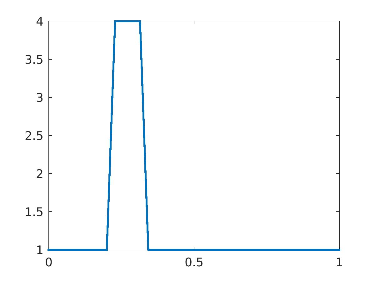
(a) True $c(x)$. The $x-$axis indicates $x\in(0,1)$

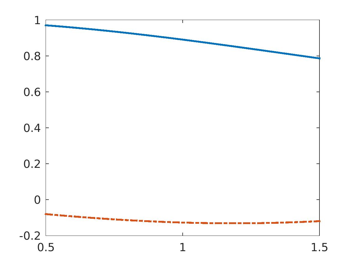
(b) The real (solid line) and imaginary parts of the data $g_{0}(k)$, defined in (2.6). The $x-$axis indicates $k\in(0.5,1.5)$.

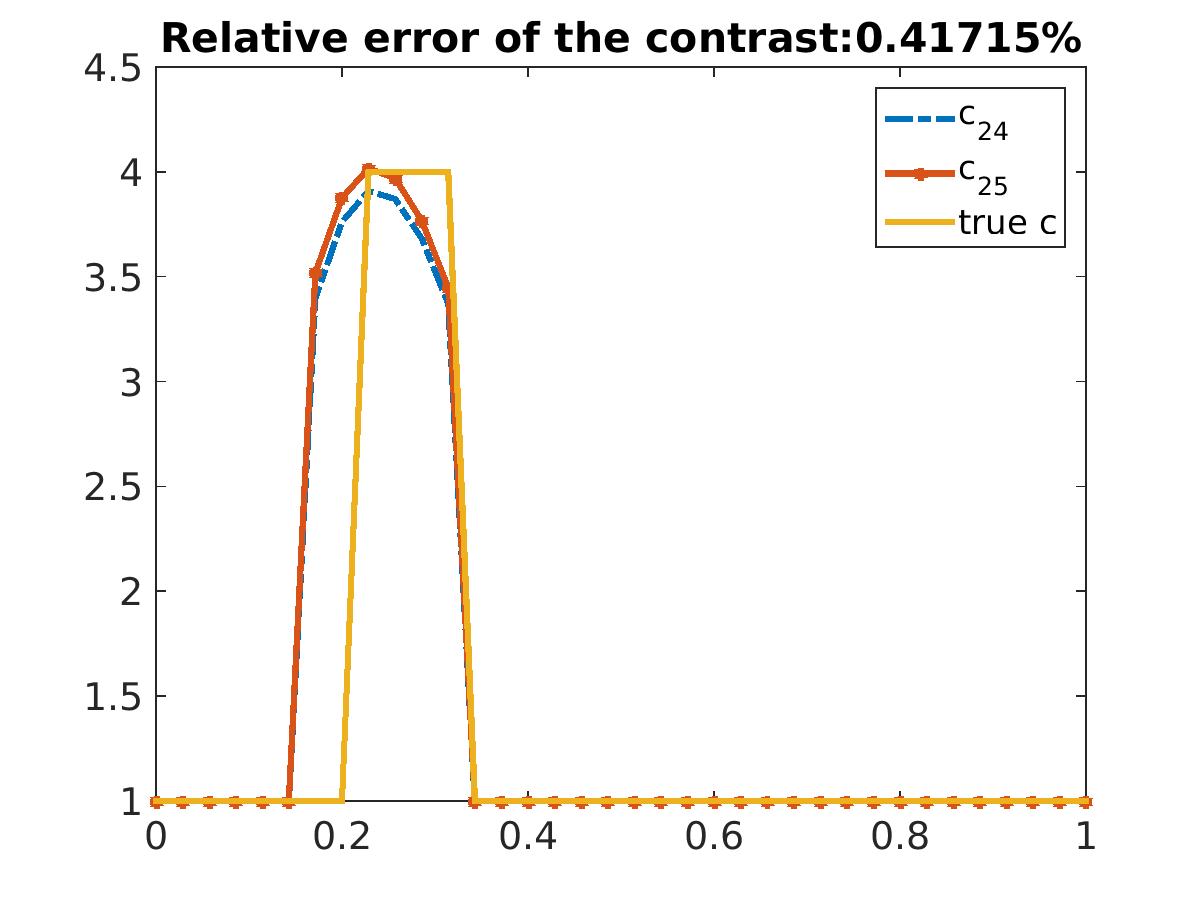
(c) The reconstruction of $c$ when $m^{0}=24,25$. The $x-$axis indicates $x\in(0,1)$.

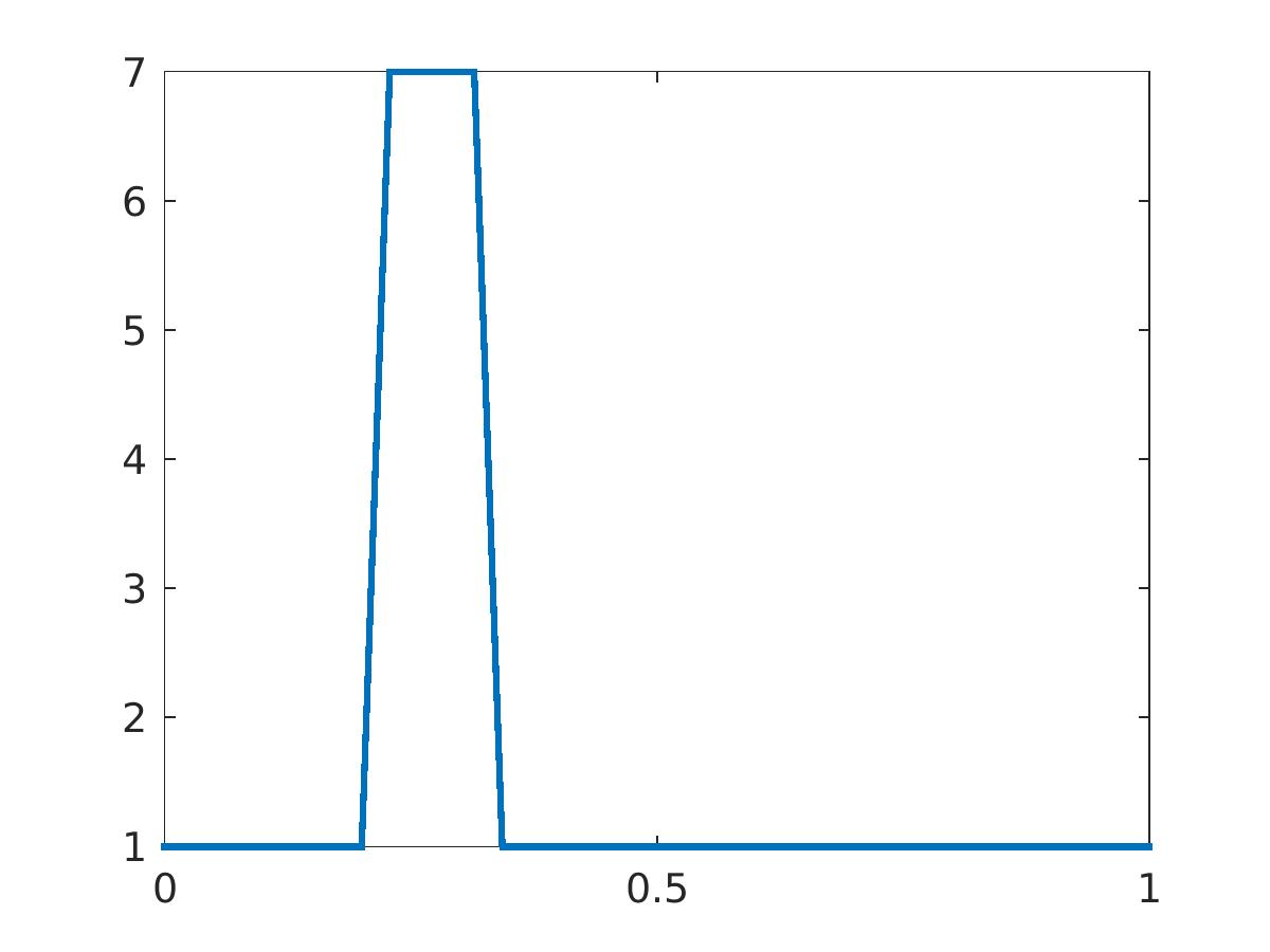
(d) True $c(x)$. The $x-$axis indicates $x\in(0,1)$

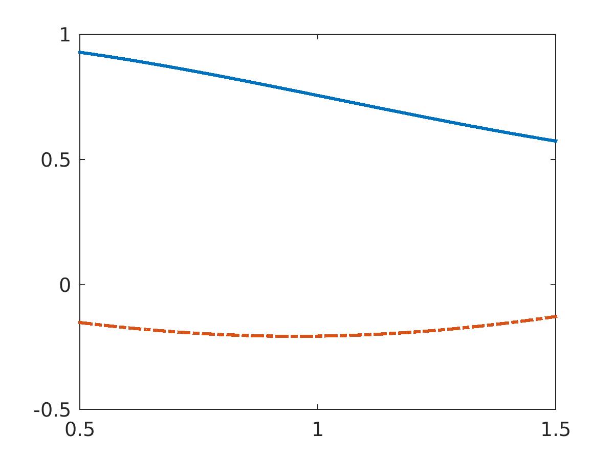
(e) The real (solid line) and imaginary parts of the data $g_{0}(k)$, defined in (2.6). The $x-$axis indicates $k\in(0.5,1.5)$.

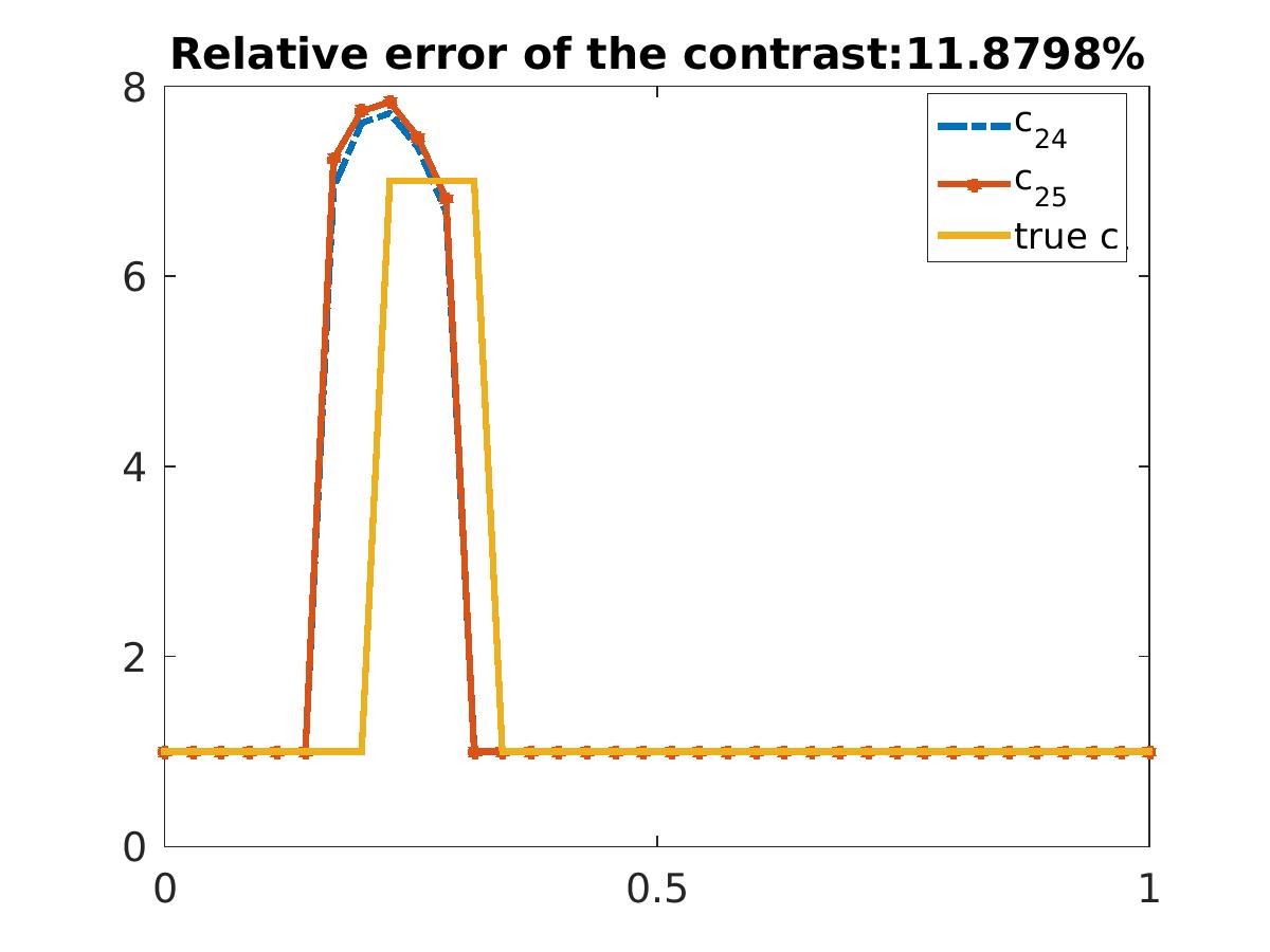
(f) The reconstruction of $c$ when $m^{0}=24,25$. The $x-$axis indicates $x\in(0,1)$.

Figure 1: Numerical results when $c_{\mathrm{target}}$ is 4 (in row 1) and 7 (in row 2). The relative error in figures (c) and (f) is $\left|\|c_{25}\|_{L^{\infty}(0,1)}-\|c^{*}\|_{L^{\infty}(0,1)}\right|/\|c^{*}\|_{L^{\infty}(0,1)}$.

Remark 6.1.

In our computer program, we use the linear algebra package, named as Armadillo [25] to solve linear systems. The software is very helpful to speed up the program and to simplify the codes.

6.2 Experimental data

The experimental data were collected by the Forward Looking Radar which was built in the US Army Research Laboratory [23]. The device consists of two main parts. The first one, emitter, generates the time resolved electric pulses. The emitter sends out only one component of the electric field. The second part involves 16 detectors. These detectors collect the time resolved backscattering electric signal (voltage) in the time domain. The same component of the electric field is measured as the one which is generated by the emitter: see our comment about this in the beginning of section 2. The step size of time is 0.133 nanosecond. The backscattering data in the time domain are collected when the distance between the radar and the target varies from 20 to 8 meters. The average of these data with respect to both the position of the radar and those 16 detectors is the data on which we have tested our algorithm. To identify horizontal coordinates of the position of the target, Ground Positioning System (GPS) is used. The error in each of horizontal coordinates does not exceed a few centimeters. When the target is under the ground, the GPS provides the distance between the radar and a point on the ground located above the target. As to the depth of a buried target, it is not of a significant interest, since horizontal coordinates are known and it is also known that the depth does not exceed 10 centimeters. We refer to [23] for more details about the data collection process. Publications [11, 18, 19] contain schematic diagrams of the measurements.

Our interest is in computing maximal values of dielectric constants of targets. In one target (plastic cylinder below) we compute the minimal value of its dielectric constant, since its value was less than the dielectric constant of the ground. For each target, the only information the mathematical team (MVK,LHN) had, in addition to just a single experimental curve, was whether it was located in air or below the ground.

We calculate $R(x),$ the relative spatial dielectric constant of the whole structure including the background (air or the ground) and the target. More precisely,

$$R(x)=\left\{\begin{array}[]{ll}\displaystyle\frac{c_{\mathrm{target}}}{c_{\mathrm{bckgr}}}&x\in D,\\ 1&\mathrm{otherwise}\end{array}\right.$$ (6.1)

where $D$ is the subinterval of the interval $\left(0,1\right),$ which is occupied by the target. Here $c_{\text{target}}$ and $c_{\text{bckgr}}$ are values of the function $c\left(x\right)$ in target and background respectively. We assume that $c_{\text{bckgr}}=const.>0$ for each set of experimental data. Hence, $c_{\mathrm{bckgr}}=1$ if the target is located in air. The ground was dry sand. It is well known that the dielectric constant of the dry sand varies between 3 and 5 [27]. Hence, in the case of buried targets $c_{\mathrm{bckgr}}\in[3,5]$.

In our mathematical model the time resolved electric signal $\widehat{u}(x,x_{0},t)$ collected by the detectors satisfies the equations (2.14), (2.15) with $c(x)$ being replaced by $R(x),$ where the position $x_{0}$ of the source is actually unknown. The latter is one of the difficulties of working with these data. Thus, we set in all our tests $x_{0}=-1,$ which is the same as in [11, 18, 19].

Let $R_{\text{comp}}(x)$ be the function $R(x)$ which we compute. Following [18], we define the computed target/background contrast as

$$\widetilde{R}=\left\{\begin{array}[]{c}\max R\left(x\right)\text{ if }R\left(x\right)\geq 1,\forall x\in\left[0,1\right],\\ \min R\left(x\right)\text{ if }0<R\left(x\right)\leq 1,\forall x\in\left[0,1\right].\end{array}\right.$$ (6.2)

Since the dielectric constant of air equals 1, then we have $R\left(x\right)\geq 1$ for targets located in air. As to the buried targets, we have developed a procedure of the analysis of the original time resolved data, which provides us with the information on which of two cases (6.2) takes place. We refer to Case 1 and Case 2 on page 2944 of [19] for this procedure. In addition, since we had a significant mismatch of magnitudes of experimental and computationally simulated data, we have multiplied, before computations, our experimental data by the calibration number $10^{-7},$ see [18, 19] for details of our choice of this number.

There is a significant discrepancy between computationally simulated and experimental data, which was noticed in our earlier publications [11, 18, 19]. This discrepancy is evident from, comparison of, e.g. Figure 1b with Figure 2b and other similar ones. Therefore, to at least somehow mitigate this discrepancy, we perform a data pre-processing procedure. Besides of the Fourier transform of the time resolved data, we multiply them by a calibration factor, truncate a certain part of the data in the frequency domain and shift the data in the frequency domain, see details below.

The function $u(0,x_{0},k),$ which we have studied in the previous sections, is the Fourier transform of the time resolved data $\widehat{u}(0,x_{0},t)$. The function $u(0,x_{0},k)$ is called “the data in the frequency domain”. Observing that $|u(0,x_{0},k)|$ is small when $k$ belongs to a certain interval, we do not analyze $u(0,x_{0},k)$ on that interval. Rather, we only focus on such a frequency interval which contains the major part of the information. Now, to keep the consistency with our study of computationally simulated data, we always force the frequency interval to be $\left[0.5,1.5\right]$. To do so, we simply shift our data in the frequency domain: compare Figures 2b and 2c, Figures 2f and 2g, Figures 3b and 3c, Figures 3f and 3g and Figures 3j and 3k.

We consider two cases: targets in air (Figure 2) and targets buried about a few centimeters under the ground (Figure 3). We had experimental data for total of five (5) targets. The reconstructed dielectric constants of these targets are summarized in Table 1. In this table, computed $c_{\text{comp}}=\widetilde{R}\cdot c_{\text{bckgr}}$. In tables of dielectric constants of materials, their values are usually given within certain intervals [27]. Now about the intervals of the true $c:=c_{\text{true}}$ in the $6^{\text{th}}$ column of Table 1. In the cases when targets were a wood stake and a plastic cylinder, we have taken those intervals from a published table of dielectric constants [27]. The interval of the true $c$ for the case when the target was bush, was taken from [7]. As to the metal targets, it was established in [18] that they can be considered as such targets whose dielectric constants belong to the interval $[10,30].$

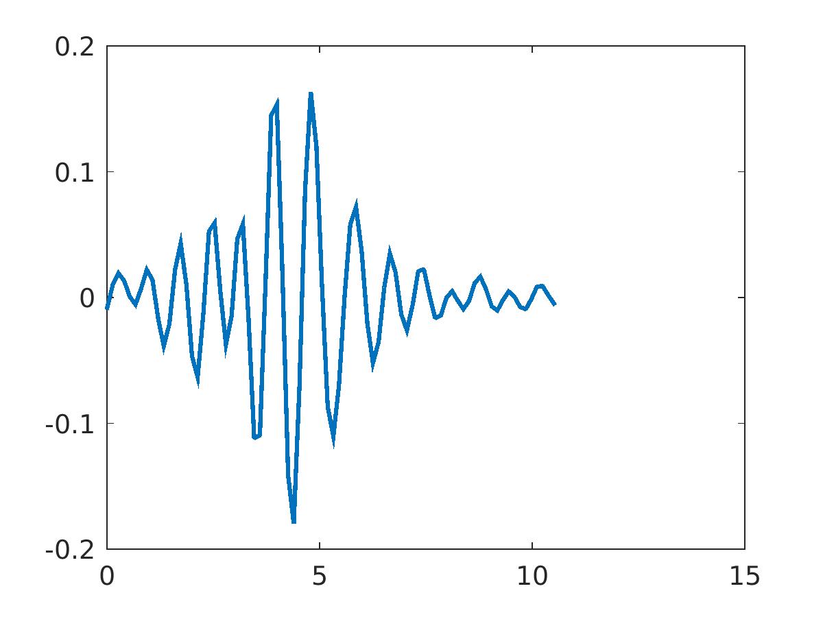
(a) The scattering field in the time domain

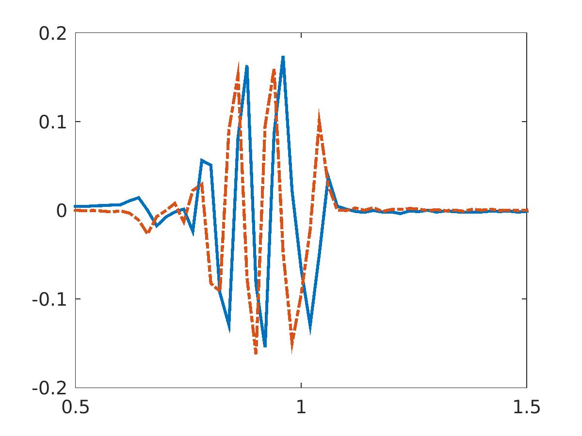
(b) The scattering field in the frequency domain

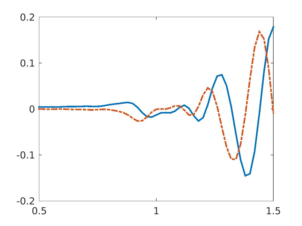
(c) The scattering field in the frequency domain after cutting off its small information

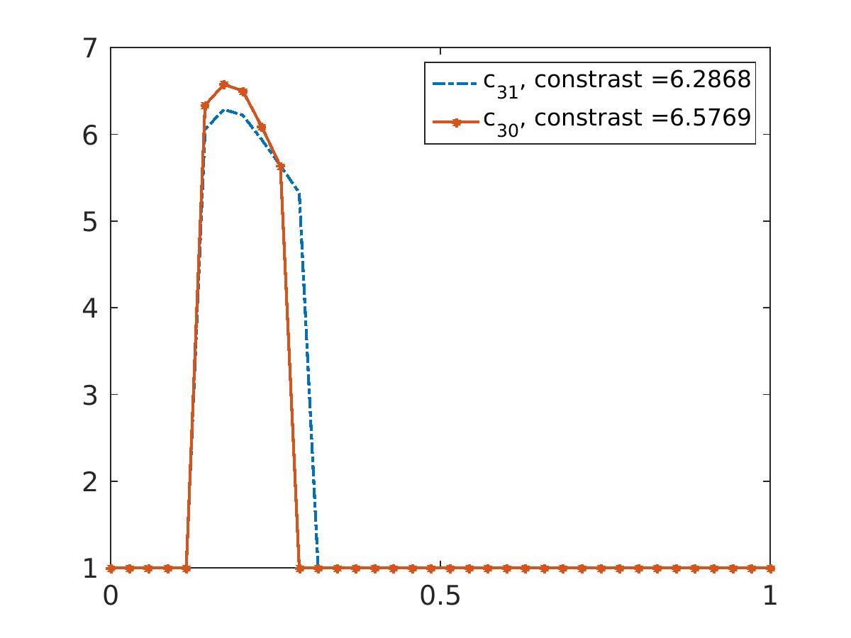
(d) The reconstruction of $R(x)$

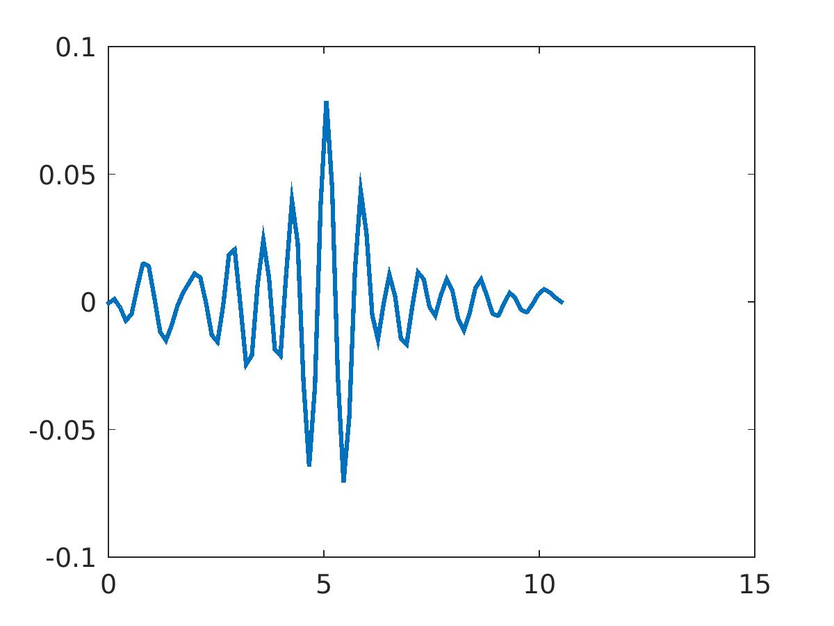
(e) The scattering field in the time domain

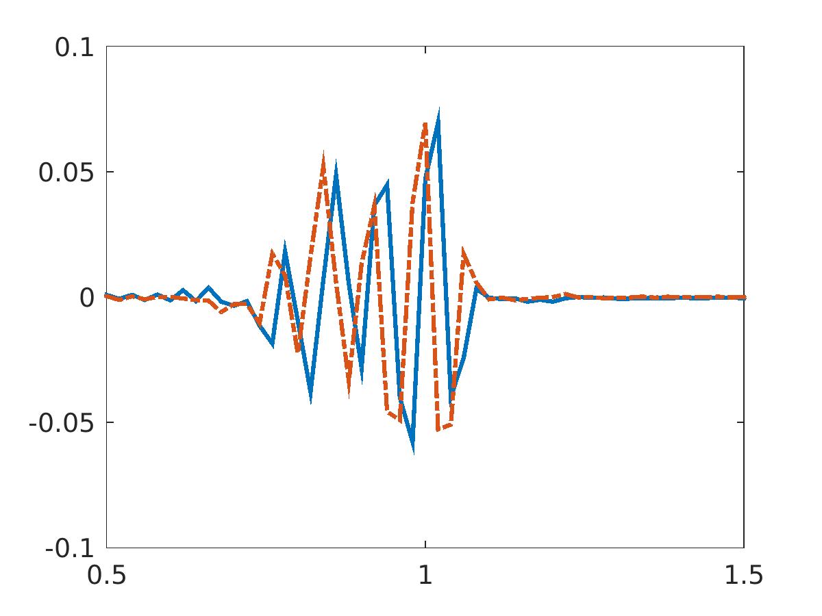
(f) The scattering field in the frequency domain

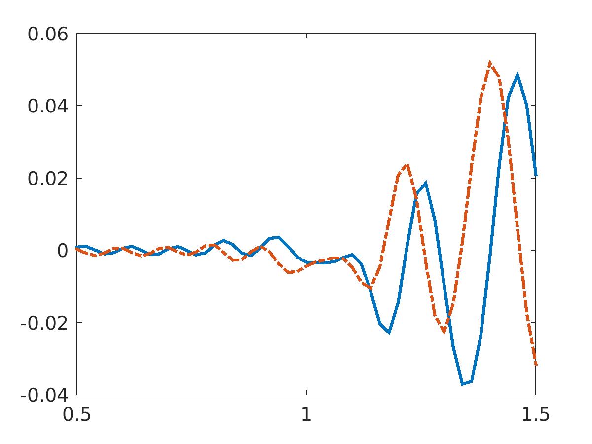
(g) The scattering field in the frequency domain after cutting off its small information

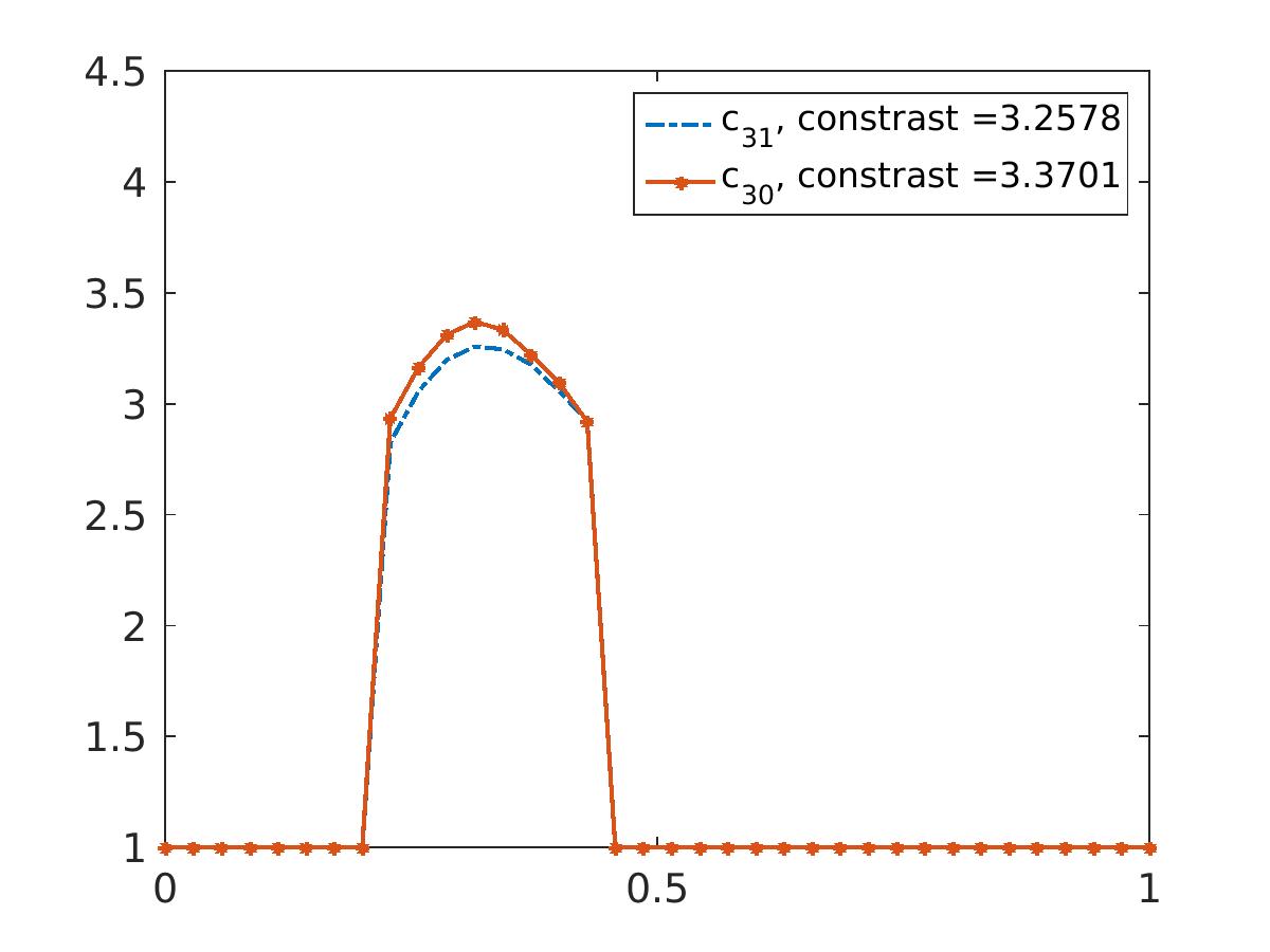
(h) The reconstruction of $R(x)$

Figure 2: The numerical test to evaluate the “relative” dielectric constant of bush (first row) and wood stake (second row) when they are put in the air. Solid lines on b,c,f,g are real parts and dotted lines are imaginary parts.

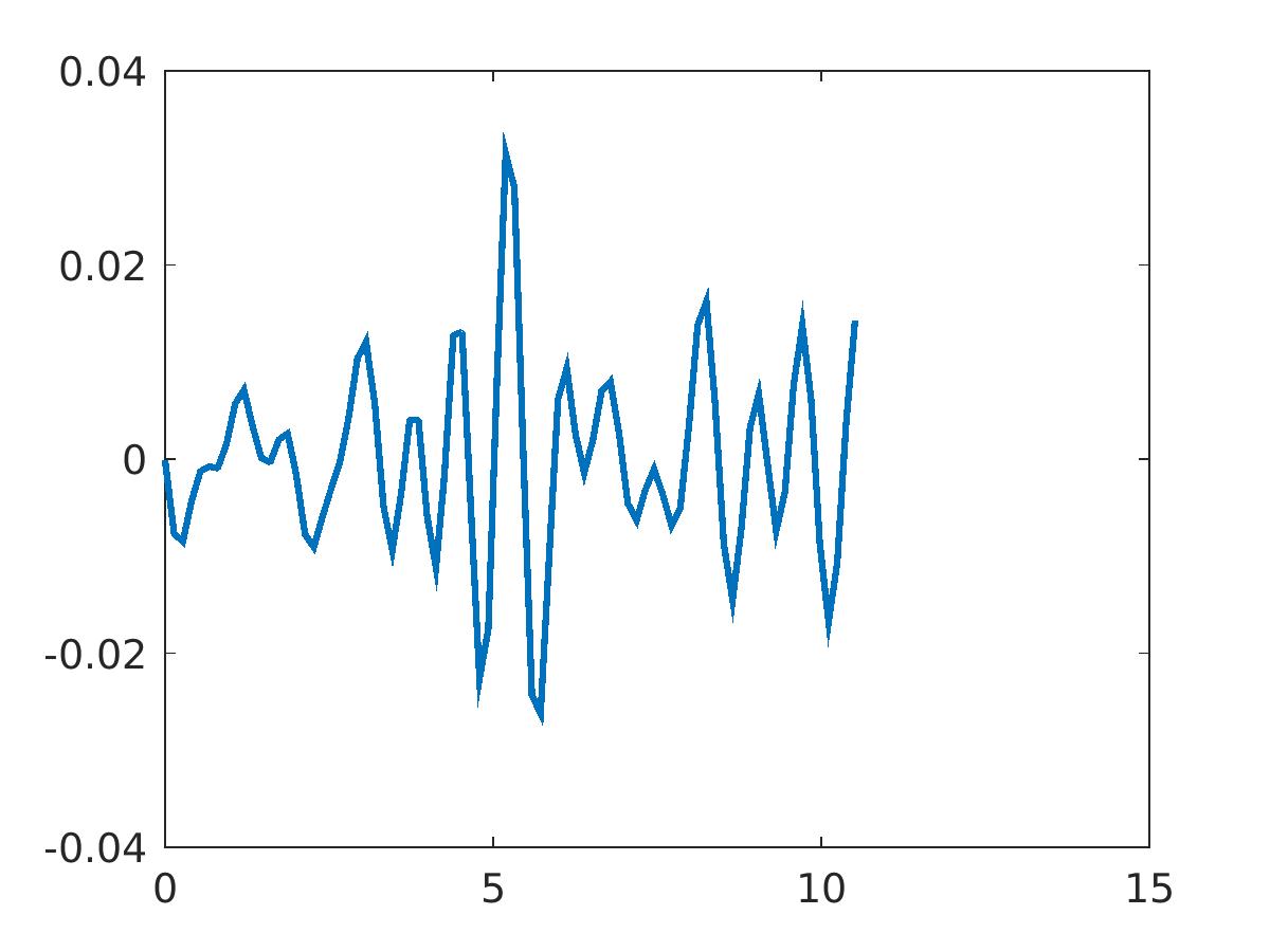
(a) The scattering field in the time domain

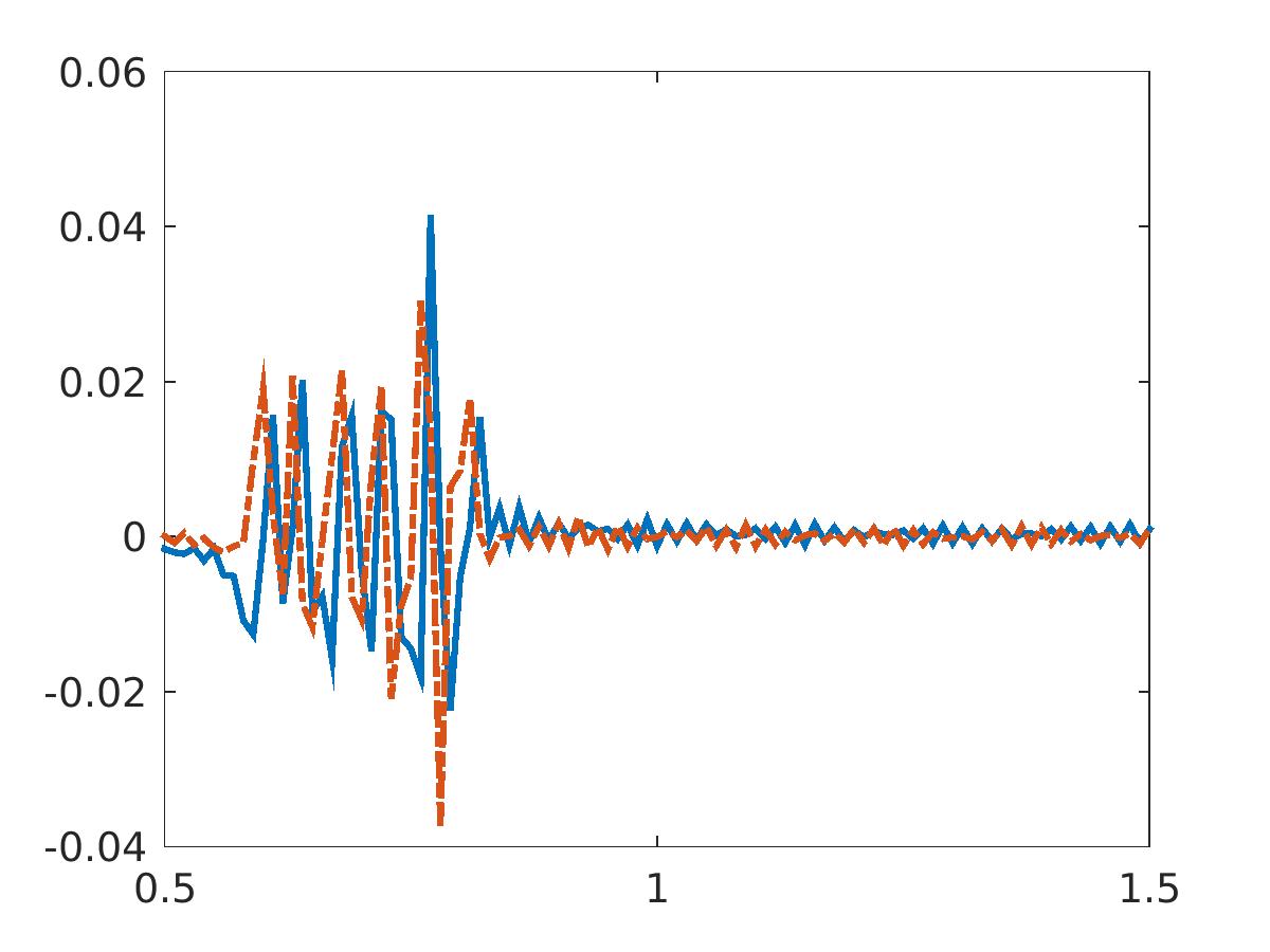
(b) The scattering field in the frequency domain

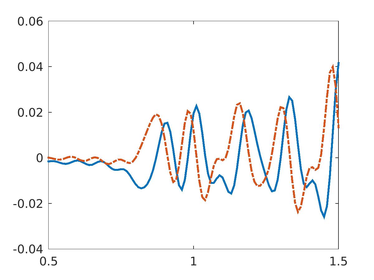
(c) The scattering field in the frequency domain after cutting off its small information

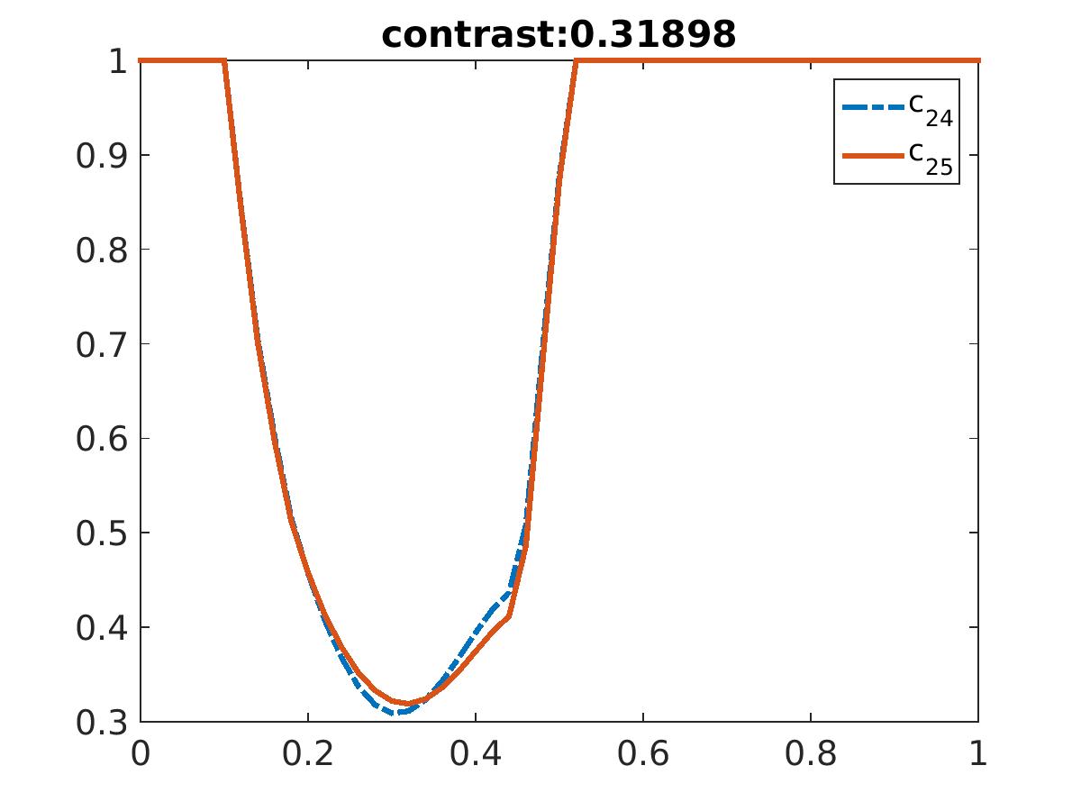
(d) The reconstruction of $R(x)$

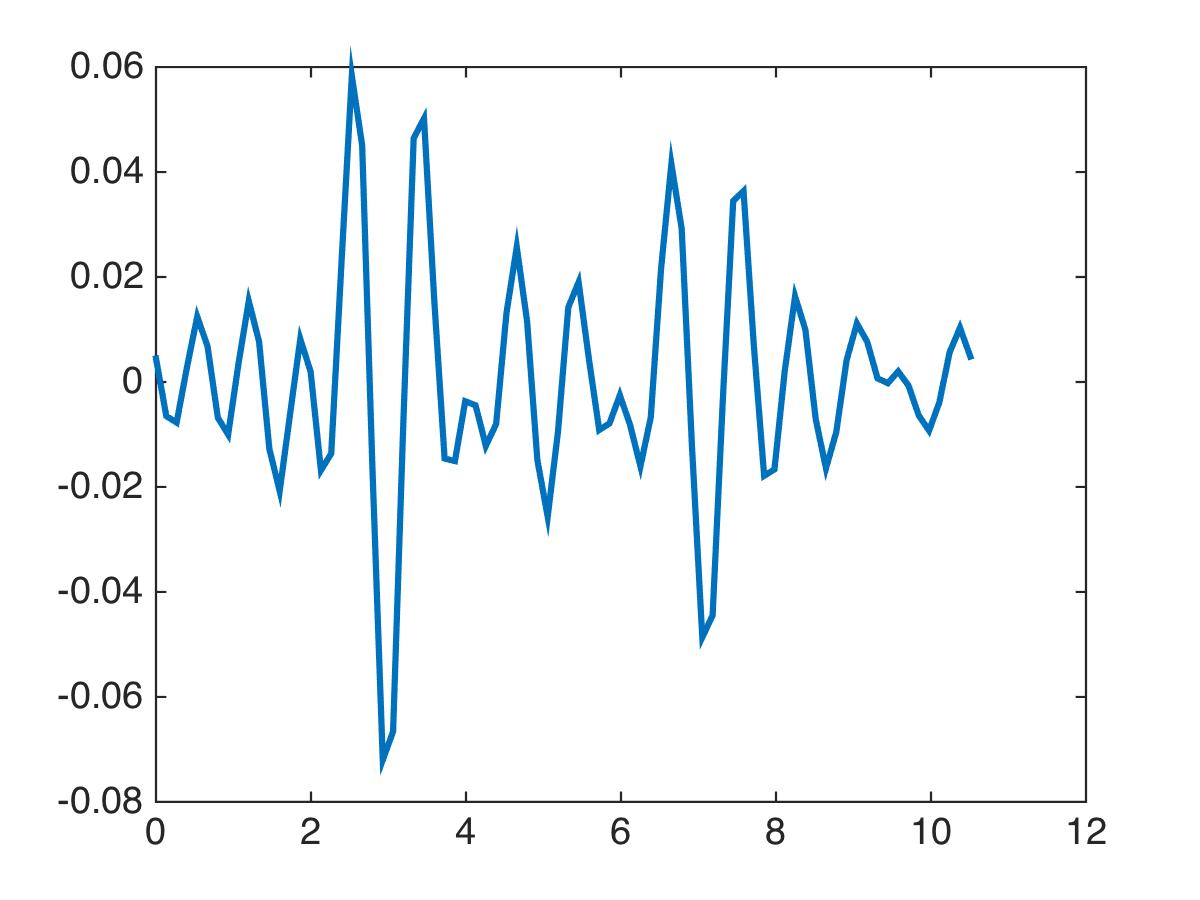
(e) The scattering field in the time domain

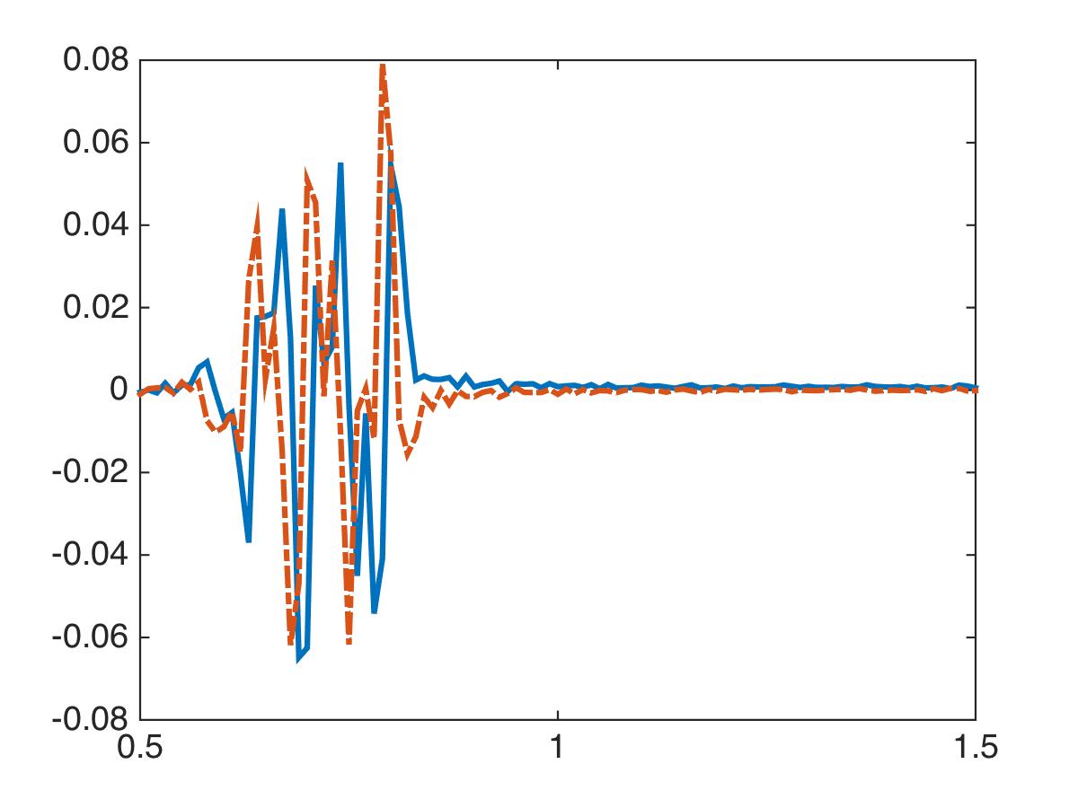
(f) The scattering field in the frequency domain

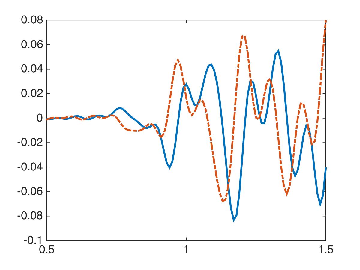
(g) The scattering field in the frequency domain after cutting off its small information

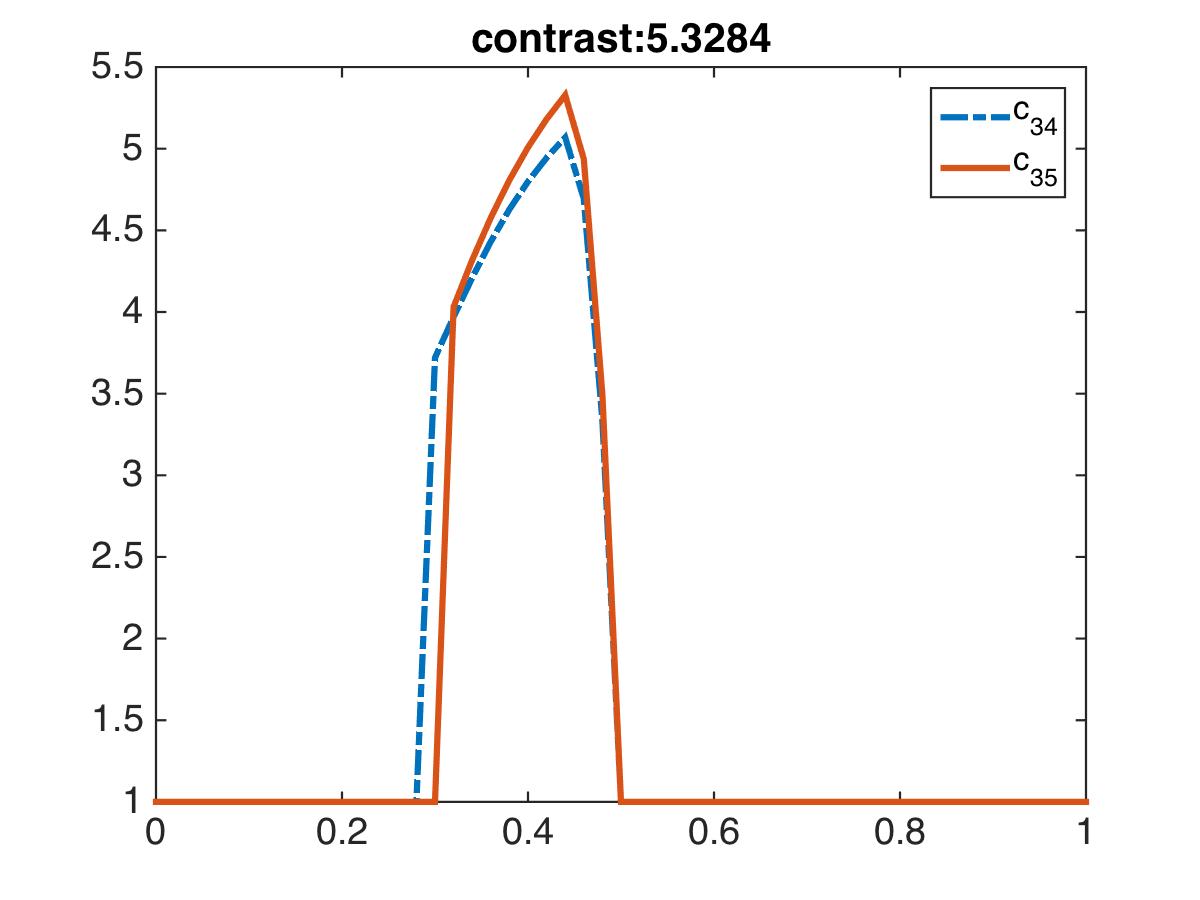
(h) The reconstruction of $R(x)$

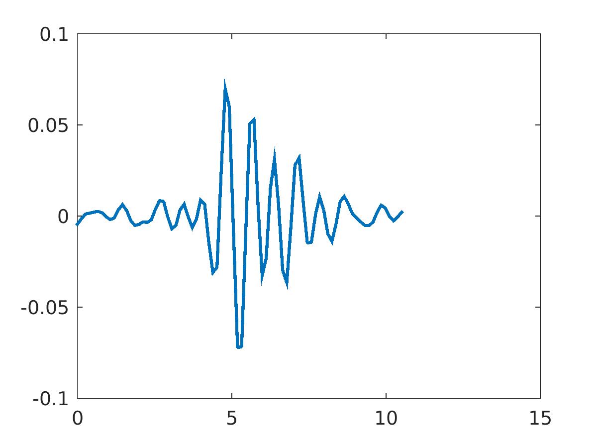
(i) The scattering field in the time domain

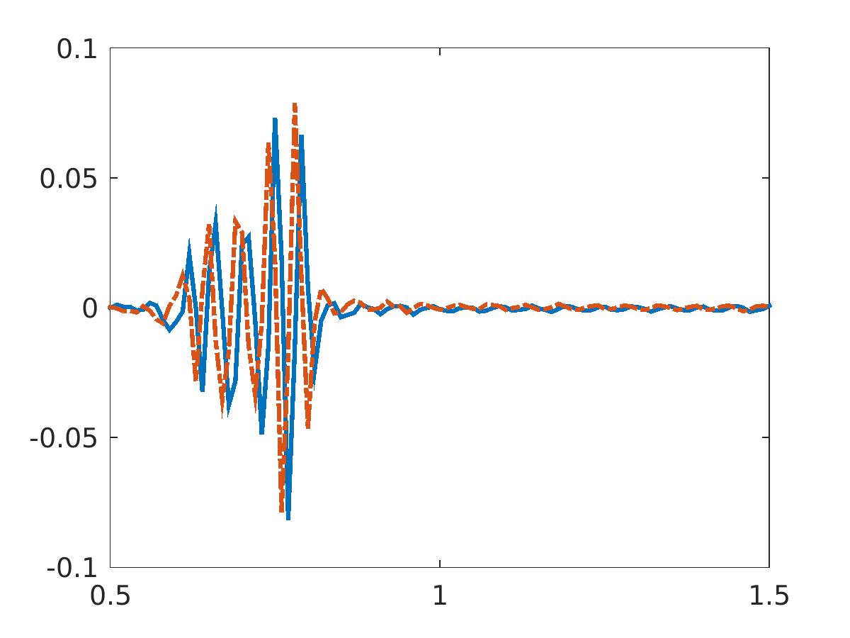
(j) The scattering field in the frequency domain

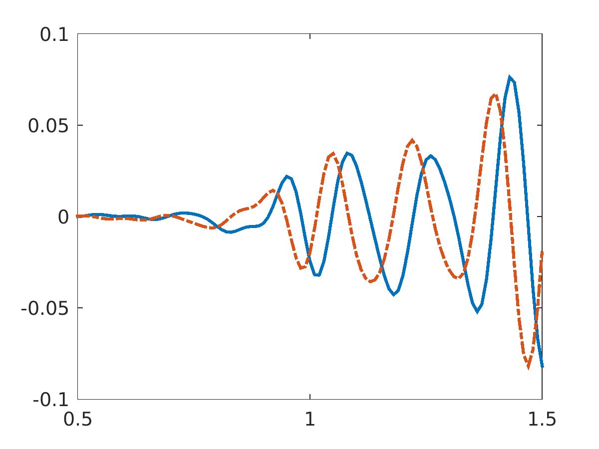
(k) The scattering field in the frequency domain after cutting off its small information

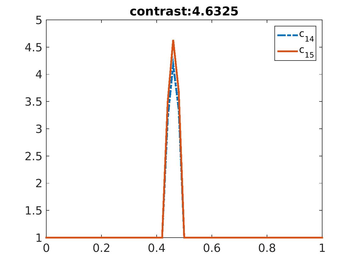
(l) The reconstruction of $R(x)$

Figure 3: The case when plastic (row 1), metal cylinder (row 2), and metal box(row 3) are buried under the ground. Solid lines on b,c,f,g,j,k are real parts and dotted lines are imaginary parts.

Table 1: Computed dielectric constants of five targets Target $c_{\mathrm{bckgr}}$ Reconstructed $\widetilde{R}$ $c_{\mathrm{bckgr}}$ $c_{\text{comp}}$ True $c_{\text{true}}$ Bush 1 6.5 1 6.5 $[3,20]$ Wood stake 1 3.3 1 3.3 $[2,6]$ Metal box 4 4.6 $[3,5]$ $[13.8,23]$ $[10,30]$ Metal cylinder 4 5.3 $[3,5]$ $[15.9,26.5]$ $[10,30]$ Plastic cylinder 4 0.3 $[3,5]$ $[0.9,1.5]$ $\left[1.1,3.2\right]$

7 Summary

In this paper, we have developed a frequency domain analog of the 1-d globally convergent method of [11, 18, 19]. We have tested this analog on both computationally simulated and time resolved experimental data. The experimental data are the same as ones used in [11, 18, 19]. We have modeled the process of electromagnetic waves propagation by the 1-d wave-like PDE. The reason why we have not used a 3-d model, as in, e.g. earlier works of this group on experimental data [1, 28, 29], is that we had only one time resolved experimental curve for each of our five targets.

Our numerical method has the global convergence property. In other words, we have proven a theorem (Theorem 5.1), which claims that we obtain some points in a sufficiently small neighborhood of the exact solution without any advanced knowledge of this neighborhood. Our technique heavily relies on the Quasi Reversibility Method (QRM). The proof of the convergence of the QRM is based on a Carleman estimate. A significant modification of our technique, as compared with [11, 18, 19], is due to two factors. First, we use the Fourier transform of time resolved data instead of the Laplace transform in [11, 18, 19]. Second, when updating tail functions via (4.25), we solve the problem (4.9), (4.10) using the QRM. On the other hand, in [11, 18, 19] tail functions were updated via solving the “Laplace transform analog” of the problem (2.3), (2.4) as a regular forward problem

Since the dielectric constants of targets were not measured in experiments, the maximum what we can do to evaluate our results is to compare them with published data in, e.g. [27]. Results of Table 1 are close to those obtained in [11, 18, 19]. One can see in Table 1 that our reconstructed values of dielectric constants are well within published limits. We consider the latter as a good result. This is achieved regardless on a significant discrepancy between computationally simulated and experimental data, regardless on a quite approximate nature of our mathematical model and regardless on the presence of clutter at the data collection site. That discrepancy is still very large even after the data pre-processing, as it is evident from comparison of Figures 1b,e with Figures 2c,g and Figures 3c,g,k. Besides, the source position $x_{0}$ was unknown but rather prescribed by ourselves as $x_{0}=-1.$ Thus, our results indicate a high degree of stability of our method.

References

• [1] L. Beilina and M.V. Klibanov, Approximate Global Convergence and Adaptivity for Coefficient Inverse Problems, Springer, New York, 2012.
• [2] L. Beilina and M.V. Klibanov, A new approximate mathematical model for global convergence for a coefficient inverse problem with backscattering data, J. Inverse and Ill-Posed Problems, 20, 512-565, 2012.
• [3] L. Beilina, Energy estimates and numerical verification of the stabilized domain decomposition finite element/finite difference approach for the Maxwell’s system in time domain, Central European Journal of Mathematics, 11, 702–733, 2013.
• [4] L. Bourgeois and J. Dardé, About stability and regularization of ill-posed elliptic Cauchy problems: the case of Lipschitz domains, Applicable Analalysis, 89, 1745-1768, 2010.
• [5] L. Bourgeois and J. Dardé, A duality-based method of quasi-reversibility to solve the Cauchy problem in the presence of noisy data, Inverse Problems, 26, 095016, 2010.
• [6] L. Bourgeois and J. Dardé, The “exterior approach” to solve the inverse obstacle problem for the Stokes system, Inverse Problems and Imaging 8, 23-51, 2014.
• [7] H.T. Chuah, K.Y. Lee and T.W. Lau, Dielectric constants of rubber and oil palm leaf samples at X-band, IEEE Trans. on Geoscience and Remote Sensing, 33, 221-223, 1995.
• [8] S. I. Kabanikhin, On linear regularization of multidimensional inverse problems for hyperbolic equations, Soviet Mathematics Doklady, 40, 579–583, 1990.
• [9] S. I. Kabanikhin, A. D. Satybaev, and M. A. Shishlenin, Direct Methods of Solving Inverse Hyperbolic Problems, VSP, Utrecht, 2005.
• [10] S.I. Kabanikhin, K.K. Sabelfeld, N.S. Novikov and M. A. Shishlenin, Numerical solution of the multidimensional Gelfand-Levitan equation, J. Inverse and Ill-Posed Problems, 23, 439-450, 2015.
• [11] A.L. Karchevsky, M.V. Klibanov, L. Nguyen, N. Pantong and A. Sullivan, The Krein method and the globally convergent method for experimental data, Applied Numerical Mathematics, 74, 111-127, 2013.
• [12] M.V. Klibanov and F. Santosa, A computational quasi-reversibility method for Cauchy problems for Laplace’s equation, SIAM J. Appl. Math., 51, 1653-1675, 1991.
• [13] M.V. Klibanov and J. Malinsky, Newton-Kantorovich method for 3-dimensional potential inverse scattering problem and stability for the hyperbolic Cauchy problem with time dependent data, Inverse Problems, 7 577-596, 1991.
• [14] M.V. Klibanov and A. Timonov, Carleman Estimates for Coefficient Inverse Problems and Numerical Applications, VSP, Utrecht, The Netherlands, 2004.
• [15] M.V. Klibanov and N. T. Thành, Recovering dielectric constants of explosives via a globally strictly convex cost functional, SIAM J. Appl. Math., 75, 528-537, 2015.
• [16] M.V. Klibanov, Carleman estimates for the regularization of ill-posed Cauchy problems, Applied Numerical Mathematics, 94, 46-74, 2015.
• [17] M. G. Krein, On a method of effective solution of an inverse boundary problem, Dokl. Akad. Nauk SSSR, 94, 987-990, 1954 (in Russian).
• [18] A.V. Kuzhuget, L. Beilina, M.V. Klibanov, A. Sullivan, L. Nguyen and M.A. Fiddy, Blind backscattering experimental data collected in the field and an approximately globally convergent inverse algorithm, Inverse Problems, 28, 095007, 2012.
• [19] A.V. Kuzhuget, L. Beilina, M.V. Klibanov, A. Sullivan, L. Nguyen and M.A. Fiddy, Quantitative image recovery from measured blind backscattered data using a globally convergent inverse method, IEEE Transaction for Geoscience and Remote Sensing, 51, 2937-2948, 2013.
• [20] R. Lattes and J.-L. Lions, The Method of Quasireversibility: Applications to Partial Differential Equations, Elsevier, New York, 1969.
• [21] D. Lesnic, G. Wakefield, B.D. Sleeman and J.R. Okendon, Determination of the index of refraction of ant-reflection coatings, Mathematics-in-Industry Case Studies Journal, 2, 155-173, 2010.
• [22] B.M. Levitan, Inverse Sturm-Liouville Problems, VSP, Utrecht, 1987.
• [23] N. Nguyen, D. Wong, M. Ressler, F. Koenig, B. Stanton, G. Smith, J. Sichina and K. Kappra, Obstacle avolidance and concealed target detection using the Army Research Lab ultra-wideband synchronous impulse Reconstruction (UWB SIRE) forward imaging radar, Proc. SPIE 6553 65530H (1)-65530H (8), 2007.
• [24] V.G. Romanov, Inverse Problems of Mathematical Physics, VNU Press, Utrecht, The Netherlands, 1986.
• [25] C. Sanderson, Armadillo: An Open Source C++ Linear Algebra Library for Fast Prototyping and Computationally Intensive Experiments, Technical Report, NICTA, 2010.
• [26] J.A. Scales, M.L. Smith and T.L. Fischer, Global optimization methods for multimodal inverse problems, J. Computational Physics, 103, 258-268, 1992.
• [27] Table of dielectric constants, https://www.honeywellprocess.com/library/marketing/tech-specs/Dielectric%20Constant%20Table.pdf.
• [28] N. T. Thành, L. Beilina, M. V. Klibanov and M. A. Fiddy, Reconstruction of the refractive index from experimental backscattering data using a globally convergent inverse method, SIAM Journal on Scientific Computing, 36, B273–B293, 2014.
• [29] N. T. Thành, L. Beilina, M. V. Klibanov and M. A. Fiddy, Imaging of buried objects from experimental backscattering time dependent measurements using a globally convergent inverse algorithm, SIAM J. Imaging Sciences, 8, 757-786, 2015.
• [30] A.N. Tikhonov, A.V. Goncharsky, V.V. Stepanov and A.G. Yagola, Numerical Methods for the Solution of Ill-Posed Problems, Kluwer, London, 1995.
• [31] B.R. Vainberg, Principles of radiation, limiting absorption and limiting amplitude in the general theory of partial differential equations, Russian Math. Surveys, 21, 115-193, 1966.
• [32] B.R. Vainberg, Asymptotic Methods in Equations of Mathematical Physics, Gordon and Breach Science Publishers, New York, 1989.
• [33] V.S. Vladimirov, Equations of Mathematical Physics, M. Dekker, New York, 1971.