Vacancy-induced low-energy states in undoped graphene

Abstract

We demonstrate that a nonzero concentration $n_{v}$ of static, randomly-placed vacancies in graphene leads to a density $w$ of zero-energy quasiparticle states at the band-center $\epsilon=0$ within a tight-binding description with nearest-neighbour hopping $t$ on the honeycomb lattice. We show that $w$ remains generically nonzero in the compensated case (exactly equal number of vacancies on the two sublattices) even in the presence of hopping disorder, and depends sensitively on $n_{v}$ and correlations between vacancy positions. For low, but not-too-low $|\epsilon|/t$ in this compensated case, we show that the density of states (DOS) $\rho(\epsilon)$ exhibits a strong divergence of the form $\rho_{\rm 1D}(\epsilon)\sim|\epsilon|^{-1}/[\log(t/|\epsilon|)]^{(y+1)}$, which crosses over to the universal low-energy asymptotic form expected on symmetry grounds $\rho_{\rm GW}(\epsilon)\sim|\epsilon|^{-1}e^{-b[\log(t/|\epsilon|)]^{2/3}}$ below a crossover scale $\epsilon_{c}\ll t$. $\epsilon_{c}$ is found to decrease rapidly with decreasing $n_{v}$, while $y$ decreases much more slowly.

Static impurities, which give rise to random time-independent terms in the single-particle Hamiltonian for quasiparticle excitations of a condensed matter system, can lead to the phenomenon of Anderson localization, whereby quasiparticle wavefunctions lose their plane-wave character and become localized Lee_Ramakrishnan . Such localization transitions and universal low-energy properties of the localized phase have been successfully described in many cases using effective field-theories Altland_Simons_Zirnbauer ; Evers_Mirlin whose form depends on symmetry properties of the quasiparticle Hamiltonian in the presence of impurities. In some cases Gade ; Gade_Wegner , it has also been possible to refine these field theoretical predictions using real-space strong-disorder renormalization group ideas Motrunich_Damle_Huse .

In this Letter, we study the effects of a nonzero concentration $n_{v}$ of static, randomly-located vacancies in graphene. We use a tight-binding description for electronic states of graphene, with hopping amplitude $t$ between nearest-neighbour sites on a honeycomb lattice, and model vacancies by the deletion of the corresponding site in this tight-binding model Araujo_Terrones_Dresselhaus ; Forte_etal ; Pereira_dosSantos_CastroNeto ; Pereira_Guinea_dosSantos_Peres_CastroNeto ; Wehling_Yuan_Lichtenstein_Geim_Katsnelson . We focus on the compensated case, i.e., exactly equal numbers of vacancies on the two sublattices of the honeycomb lattice, and demonstrate that vacancies generically lead to a nonuniversal density $w$ of zero-energy quasiparticle states at the band-center $\epsilon=0$ even in this compensated case, including in the presence of hopping disorder. For low, but not-too-low $|\epsilon|/t$ in this compensated case, the density of states (DOS) $\rho(\epsilon)$ exhibits a strong divergence of the form:

$$\rho_{\rm 1D}(\epsilon)\sim|\epsilon|^{-1}/[\log(t/|\epsilon|)]^{(y+1)}\;,$$ (1)

familiar in the context of various random-hopping problems in one dimension Dyson ; Theodorou_Cohen ; Eggarter_Riedenger ; Motrunich_Damle_Huse_PRB0 ; Motrunich_Damle_Huse_PRB1 ; Gruzberg_Read_Vishweshwara ; Brouwer_Furusaki_Gruzberg_Mudry ; Brouwer_Mudry_Furusaki ; Titov_Brouwer_Furusaki_Mudry . At still lower energies, below a crossover scale $\epsilon_{c}$ that is several orders of magnitude smaller than $t$ even for moderately small values of $n_{v}$ ($0.05$–$0.1$), we show that the DOS crosses over to the low-energy asymptotic behaviour Gade ; Gade_Wegner ; Motrunich_Damle_Huse ; Mudry_Ryu_Furusaki of the chiral orthogonal universality class (to which our tight-binding model belongs on symmetry grounds):

$$\rho_{\rm GW}(\epsilon)\sim|\epsilon|^{-1}e^{-b[\log(t/|\epsilon|)]^{2/3}}\;.$$ (2)

The density of zero-energy states $w$ depends sensitively on correlations between vacancies and decreases as $n_{v}$ is lowered. The crossover energy $\epsilon_{c}$ is found to decrease rapidly with decreasing $w$, while $y$ (in fits to Eq. (1) for $|\epsilon|>\epsilon_{c}$) decreases much more slowly. On comparing the corresponding crossover length scale $l_{c}$, defined as the mean spatial separation between nonzero energy modes with $|\epsilon|<\epsilon_{c}$, with $l_{w}\equiv w^{-1/2}$, the mean spatial separation between zero-energy states, we find that $l_{c}$ tracks $l_{w}$ up to a nonuniversal prefactor. Thus, our results imply that the $w\rightarrow 0$ limit of the DOS is singular and does not commute with the $\epsilon\rightarrow 0$ limit: For any $w>0$, the true asymptotic form $\rho_{\rm GW}(\epsilon)$ cannot be obtained from an extrapolation of results obtained for $\epsilon_{c}<\epsilon\ll t$, which instead reflect the intermediate-energy physics encoded in the form $\rho_{\rm 1D}(\epsilon)$.

Our work sheds light on an interesting question motivated by the results of Willans et. al., who found a vacancy-induced DOS of the form $\rho_{\rm 1D}(\epsilon)$ at not-too-low energies in their study of Majorana excitations of Kitaev’s honeycomb model Willans_Chalker_Moessner_PRB : Does a nonzero vacancy density lead to low-energy properties qualitatively different from the asymptotic behaviour expected in the chiral orthogonal universality class of quasiparticle localization? In recent work that addressed this question in the context of graphene Hafner_etal ; Ostrovsky_etal , it was argued that vacancies lead to a new term in the low-energy field theory, which causes the DOS to take on the form $\rho_{\rm 1D}(\epsilon)$, Eq. (1), with $y=1/2$ at asymptotically low energies, rather than the asymptotic form $\rho_{\rm GW}(\epsilon)$, Eq. (2), expected on symmetry grounds.

Clearly, our conclusion is quite different, and raises two perhaps more interesting questions: When $\epsilon_{c}\ll t$, are the crossover exponent $y$ and crossover energy $\epsilon_{c}$ “universally” determined by the zero-mode density $w$, although the function $w(n_{v})$ itself depends sensitively on microscopic details such as correlations between vacancies? Can this crossover be understood within a renormalization group description of the low-energy physics? Leaving these interesting questions for future work, we devote the remainder of this Letter to an account of the calculations that lead us to our results, and thence, to these questions.

We choose the lattice spacing of the honeycomb lattice as our unit of length and measure all energies in terms of the hopping amplitude $t$, which is set by the bandwidth of the $\pi$-band of undoped graphene. We focus on the compensated case, with exactly $n_{v}L^{2}$ vacancies placed randomly on each sublattice of a finite $L\times L$ honeycomb lattice with $L^{2}$ unit cells ($2L^{2}$ sites). The spectrum of single-particle states can be obtained by diagonalizing the real symmetric matrix $H$

$$H=\left(\begin{array}[]{cc}0&T_{AB}\\ T^{\dagger}_{AB}&0\end{array}\right)$$ (3)

where $T_{AB}$ is the $(1-n_{v})L^{2}$-dimensional matrix of amplitudes for hopping from the undeleted sites of the $B$ sublattice to their undeleted $A$ sublattice neighbours, and $T^{\dagger}_{AB}$ is the transpose of this matrix (the spin label of the electronic quasiparticles is dropped since we do not study magnetic properties or sources of spin-flip scattering in this Letter).

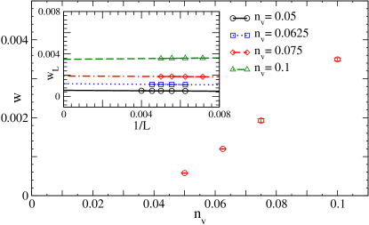
Figure 1: $w_{L}$, the density of zero modes in an $L\times L$ sample, tends to a nonzero thermodynamic limit $w$ that depends on $n_{v}$, the concentration of vacancies.

The purely off-block-diagonal form of $H$ reflects the “chiral” symmetry of the problem, corresponding to the bipartite structure of the honeycomb lattice, which guarantees that every eigenstate with energy $\epsilon>0$ has a corresponding eigenstate at energy $-\epsilon$. In order to eliminate zero modes of $H$ in the pure $L\times L$ lattice Lieb_Loss ; Ryu_Hatsugai ; Brey_Fertig , we choose even values of $L$ and impose antiperiodic boundary conditions along the $\hat{x}$ direction, while terminating the lattice in the $\hat{y}$ direction in a pair of armchair edges. We also impose a nearest-neighbour and next-nearest-neighbour exclusion constraint on the vacancies, and do not allow them to interrupt the armchair edges. These restrictions, along with the compensated nature of the vacancy disorder, eliminate all previously studied and well-understood sources of vacancy-induced Pereira_dosSantos_CastroNeto ; Brouwer_Racine_Furusaki_Hatsugai_Morita_Mudry zero modes in the spectrum of $H$.

We find it convenient to focus on the symmetric matrix $T^{\dagger}_{AB}T_{AB}$, which has a single eigenvalue $\epsilon^{2}$ for every pair of nonzero eigenvalues $(\epsilon,-\epsilon)$ of $H$. Zero modes of $T^{\dagger}_{AB}T_{AB}$, with wavefunction living entirely on the $B$ sublattice, map on to exactly half of the zero modes in the spectrum of $H$, while zero modes of the symmetric matrix $T_{AB}T^{\dagger}_{AB}$, with wavefunction living entirely on the $A$ sublattice, make up the other half of the null space of $H$. We use the ALGOL ALGOL routines of Martin and Wilkinson Martin_Wilkinson to compute the number ${\mathcal{N}}_{\Lambda}$ of eigenvalues of the banded matrix $T^{\dagger}_{AB}T_{AB}$ which are smaller in magnitude than some positive number $t^{2}\times 10^{-\Lambda}$. Our implementation Sanyal_Thesis uses calls to the GNU multiprecision library GMP for all arithmetic operations, including comparison of the magnitudes of two numbers, and has been benchmarked against routines from the LAPACK library LAPACK as well as C-translations (used in earlier work Motrunich_Damle_Huse ) of the ALGOL routines of Martin and Wilkinson.

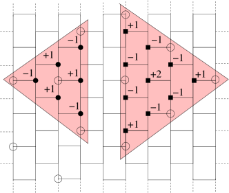
Figure 2: Four $B$-sublattice (six $A$-sublattice) vacancies arranged in a “4-triangle” pattern (“${\mathcal{R}}_{6}$” motif) give rise to a zero mode of $H$ living on $A$-sublattice sites ($B$-sublattice sites) within the 4-triangle (${\mathcal{R}}_{6}$ motif). While hopping disorder eliminates the 4-triangle zero mode, it only changes the wavefunction of the ${\mathcal{R}}_{6}$ zero mode without changing its energy.

Anticipating that the physics of interest to us spans many orders of magnitude in energy $\epsilon$, we define the ‘log-energy’ $\Gamma=\log_{10}(t/|\epsilon|)$, and compute $N^{(i)}_{\rm tot}(\Gamma,L)\equiv{\mathcal{N}}^{(i)}_{\Lambda=2\Gamma}/L^{2}$ for the $i^{th}$ $L\times L$ random sample using values of log-energy drawn from an equispaced grid ranging from $\Gamma\sim 1$ to $\Gamma\sim 100$. For large enough $\Gamma$, $N^{(i)}_{\rm tot}(\Gamma,L)$ plateaus out to a constant value which represents the density of zero modes $w^{(i)}_{L}$ of that sample. For not-too-small $n_{v}$ ($n_{v}\geq 0.05$) for which we are able to access this plateau, we separately keep track of $w_{L}^{(i)}$ and $N_{L}^{(i)}(\Gamma)\equiv N^{(i)}_{\rm tot}(\Gamma,L)-w^{(i)}_{L}$. From the position, $\Gamma_{\rm g}^{(i)}(L)$, of the last downward step in $N^{(i)}_{\rm tot}(\Gamma,L)$, we also obtain the spectral gap $\epsilon^{(i)}_{\rm g}(L)\equiv t\times 10^{-\Gamma^{(i)}_{\rm g}(L)}$ corresponding to the lowest pair of nonzero eigenvalues $\pm\epsilon^{(i)}_{\rm g}$ for that sample. Analyzing this data for up to $3000$ samples for each value of $L$ and $n_{v}$, we obtain statistically reliable estimates of the corresponding disorder-averaged quantities $w_{L}$ and $N_{L}(\Gamma)$. The density of states $\rho_{L}(\epsilon)$ can then be obtained from $N_{L}$ using the relation $\rho_{L}(\epsilon)\equiv\frac{1}{2\epsilon}\frac{dN_{L}}{d\Gamma}$. Additionally, we estimate $f_{L}$, the probability that an $L\times L$ sample has at least one pair of zero modes, and measure the histogram of $\Gamma_{\rm g}(L)$. The position of the peak in the latter provides us an estimate of $\Gamma_{\rm g}^{*}(L)$, the most probable value of $\Gamma_{\rm g}(L)$. For the smallest values of $n_{v}$, which require multiprecision computation at impracticably large $\Gamma$ in order to access the plateau in $N^{(i)}_{\rm tot}(\Gamma,L)$ (and thence, $w_{L}^{i}$), we instead compute $\frac{dN_{L}}{d\Gamma}$ by numerical differentiation of $N^{(i)}_{\rm tot}(\Gamma,L)$.

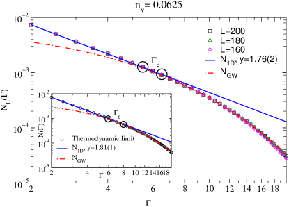
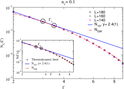
Figure 3: $N_{L}(\Gamma)$ at the three largest values of $L$ studied for $n_{v}=0.0625$ and $n_{v}=0.1$. Insets show $N(\Gamma)$ obtained by extrapolation to the thermodynamic limit. Circles demarcate the crossover region centered at the crossover scale $\Gamma_{c}$. Data for $\Gamma\lesssim\Gamma_{c}$ fits well to power-law form $N_{\rm 1D}(\Gamma)$ with the values of $y$ indicated in each case, while the large-$\Gamma$ regime fits well to the modified Gade-Wegner form $N_{\rm GW}(\Gamma)$.

Extrapolating our results for $f_{L}$ (Supplemental Material Section) and $w_{L}$ (Fig. 1) to obtain $f\equiv\lim_{L\rightarrow\infty}f_{L}$ and $w\equiv\lim_{L\rightarrow\infty}w_{L}$, we find that $f=1$, and that $w$ depends sensitively on $n_{v}$ (Fig. 1). To understand these results, we observe that $T_{AB}T^{\dagger}_{AB}$ ($T^{\dagger}_{AB}T_{AB}$) must have a zero mode, with wavefunction shown in Fig. 2, if four of the $B$-sublattice vacancies (six of the $A$-sublattice vacancies) are arranged in the specific “4-triangle” pattern (“${\mathcal{R}}_{6}$ motif”) shown in Fig. 2, with no restrictions on the positions of the other vacancies. $H$ must therefore have a pair of zero modes if a single 4-triangle or ${\mathcal{R}}_{6}$ motif occurs anywhere in the sample on either sublattice. Since there is a nonzero probability of finding a 4-triangle at a given location, this already implies that a large enough sample will certainly have at least one zero mode, i.e., $f=1$. Additionally, one has an elementary lower-bound on $w_{L}^{(i)}$ in terms of the numbers $N_{\Delta_{4A}}^{(i)}$ and $N_{\Delta_{4B}}^{(i)}$ of 4-triangles on $A$ and $B$ lattices in a given sample: $w_{L}^{(i)}\geq\left[{\rm max}(N_{\Delta_{4A}}^{(i)},N_{\Delta_{4B}}^{(i)})\right]/L^{2}$, implying $w\geq n_{\Delta_{4}}$, where $n_{\Delta_{4}}$ is the ensemble averaged concentration of 4-triangles in the thermodynamic limit. When the vacancies obey the exclusion constraints described earlier, it is not possible to produce a similar zero mode with fewer than four vacancies (Supplemental Material Section). Thus, we expect $w\sim n_{v}^{4}$ in the $n_{v}\rightarrow 0$ limit.

While our lower bound can be strengthened somewhat by including larger versions of the 4-triangle motif (Supplemental Material Section), they do not change this limiting behaviour. However, our results (Fig. 1) suggest that this limiting behaviour sets in only for $n_{v}\ll 0.05$, for which a direct computation of $w$ would require access to impracticably large $\Gamma$. For $n_{v}\gtrsim 0.05$, 4-triangles are not the dominant contribution to $w$ (Supplemental Material Section), which we expect arises instead from generalizations of the ${\mathcal{R}}_{6}$ motif: Such “${\mathcal{R}}$-type” regions have more undeleted sites belonging to one sublattice than the other, but are connected to the rest of the lattice only via sites belonging to the other sublattice. Like the ${\mathcal{R}}_{6}$ zero mode, all such ${\mathcal{R}}$-type zero modes are robust to disorder in the nearest-neighbour hopping amplitudes (Supplemental Material Section). Unlike zero modes associated with specific patterns like 4-triangles, these ${\mathcal{R}}$-type zero modes cannot be eliminated by any additional local constraints on the vacancy positions. They are therefore a generic feature of the diluted graphene lattice. Thus we see that a nonzero concentration $n_{v}$ of vacancies leads to a density $w$ of zero modes of $H$, where $w$ depends sensitively on $n_{v}$, and on correlations in the positions of vacancies, but remains generically nonzero even in the compensated case, including in the presence of hopping disorder.

Figure 3 displays $N_{L}(\Gamma)$ for $n_{v}=0.0625$ and $n_{v}=0.1$ for the three largest sizes used in our extrapolations to the thermodynamic limit. Since we expect finite-size effects to dominate for $\Gamma>\Gamma_{\rm g}^{*}(L)$, we estimate $\Gamma_{\rm g}^{*}(L)$ from histograms of $\Gamma_{\rm g}(L)$ (Supplemental Material Section) and restrict attention to $\Gamma<\Gamma_{\rm g}^{*}(L_{\rm min})$, where $L_{\rm min}$, the smallest of the sizes used in our extrapolations, is chosen large enough that $f_{L_{\rm min}}\approx 1$ in order to ensure that the physics of zero modes is correctly captured in all our analysis. In this range of $\Gamma$, we can reliably extrapolate (see Supplemental Material Section) from our data to obtain the thermodynamic limit $N(\Gamma)$ displayed in the inset of Fig. 3. Up to a fairly well-defined and readily-identified crossover scale $\Gamma_{c}(L)\equiv\log_{10}(t/|\epsilon_{c}(L)|)$, $N_{L}(\Gamma)$ is found to fit well to a power-law form $N_{\rm 1D}(\Gamma)\equiv c\Gamma^{-y}$. However, for larger $\Gamma$ beyond $\Gamma_{c}$, the asymptotic fall-off is clearly faster than a power law. $\Gamma_{c}(L)$ increases slightly with $L$ over the range of $L$ studied, but saturates at large $L$ to a finite thermodynamic limit $\Gamma_{c}$ that marks the presence of the same crossover in the limiting curve $N(\Gamma)$. Thus, $N(\Gamma)$ is again fit well by the power-law form $N_{\rm 1D}$ for $\Gamma\lesssim\Gamma_{c}$, but falls off much faster in the large-$\Gamma$ regime.

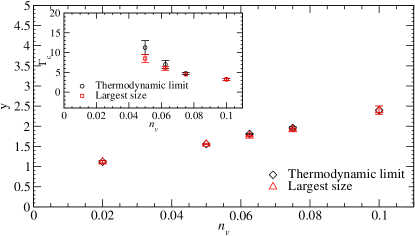
Figure 4: $n_{v}$ dependence of crossover scale $\Gamma_{c}$ and power-law exponent $y$ for samples with compensated random dilution.

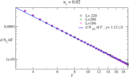
Figure 5: $\frac{dN_{L}(\Gamma)}{d\Gamma}$ at $n_{v}=0.02$ in the crossover regime converges to the thermodynamic limit for $L\sim 200$ and fits well to the form $\frac{dN_{\rm 1D}(\Gamma)}{d\Gamma}$, with a value of $y$ consistent with the trends established at larger $n_{v}$ for $\Gamma_{c}$ and $y$ (Fig. 4). Based on these trends, we expect $N(\Gamma)$ to cross over to the asymptotic form $N_{\rm GW}$ at much larger values of $\Gamma$, for which we are unable to reliably compute $N(\Gamma)$ due to computational constraints.

Given that $H$ belongs to the chiral orthogonal universality class, standard universality arguments predict that $N(\Gamma)$ and $N_{L}(\Gamma)$ should, at large enough $\Gamma$, follow the modified Gade-Wegner form Gade ; Gade_Wegner ; Motrunich_Damle_Huse ; Mudry_Ryu_Furusaki $N_{\rm GW}(\Gamma)\equiv a\Gamma^{1/3}e^{-b\Gamma^{2/3}}$.

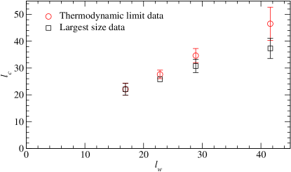
Figure 6: The crossover length-scale $l_{c}\equiv N(\Gamma_{c})^{-1/2}$ tracks the mean spatial separation $l_{w}\equiv w^{-1/2}$ between zero modes reasonably well for compensated random dilution. From left to right, the exhibited data points correspond to vacancy densities $0.1$, $0.075$, $0.0625$, and $0.05$.

From Fig. 3, we see that this form indeed provides a very good fit in the asymptotic large-$\Gamma$ regime. The same crossover is also visible at $n_{v}=0.05$ and $n_{v}=0.075$. From Fig. 4, we see that $y$ decreases gradually with $n_{v}$, while $\Gamma_{c}$ increases extremely rapidly as we go to smaller values of $n_{v}$, thereby limiting our ability to directly study this crossover for $n_{v}\lesssim 0.05$. However, one can nevertheless reliably compute the exponent $y$ that characterizes the behaviour of $\rho(\epsilon)$ in the intermediate regime $t\gg|\epsilon|\gg\epsilon_{c}$ (Fig. 5), and confirm that its value evolves smoothly (Fig. 4) down to these small values of $n_{v}$. This strongly suggests that the crossover identified by us is an intrinsic and generic feature of the density of states for any nonzero $n_{v}$.

The corresponding crossover length scale $l_{c}\equiv N(\Gamma_{c})^{-1/2}$, which represents the mean spatial separation between nonzero energy modes with $|\epsilon|/t<10^{-\Gamma_{c}}$, grows relatively slowly (Fig. 6) as $w$ is decreased, with $l_{c}\lesssim 50$ lattice units even at the smallest value of $w$ studied (corresponding to $n_{v}=0.05$). This explains why our extrapolations to the thermodynamic limit using finite-size data with $L\sim 200$ remain reliable for all $n_{v}$ studied. From Fig. 6, which compares $l_{c}$ for the randomly diluted samples with $l_{w}\equiv w^{-1/2}$, the mean spatial separation between zero modes, we also see that $l_{c}$ tracks $l_{w}$ (up to a nonuniversal prefactor). This suggests that the crossover identified in this Letter is controlled primarily by the density of zero modes. Additional support for this idea comes from our study of samples diluted with an equal number of randomly placed 4-triangles (instead of individual vacancies) on each sublattice (Supplemental Material Section), which show the same crossover, but with very different values of $\epsilon_{c}$ and $y$ that are better predicted by the zero mode density $w$ as opposed to the vacancy density. This then leads us to the questions identified earlier: Is the physics of this crossover “universally controlled” by the value of $w$ (i.e., independent of correlations between vacancy-positions and other microscopic details) in the limit of small $w$, and can it be understood via a renormalization group description of the low-energy physics?

Acknowledgements We thank M. Barma and D. Dhar for useful comments on a previous draft, and gratefully acknowledge use of computational resources funded by DST (India) grant DST-SR/S2/RJN-25/2006, in addition to departmental computational resources of the Dept. of Theoretical Physics of the TIFR. KD and OM gratefully acknowledge hospitality of ICTS-TIFR (Bengaluru) and IISc (Bengaluru) during completion of part of this work. SS gratefully acknowledges funding from DST (India) and DAE -SRC (India) and support from IISc (Bengaluru) during completion of part of this work. OM also acknowledges support by the NSF through grant DMR-1206096.

Appendix A Supplemental Material for “Vacancy-induced low-energy states in undoped graphene”

In this Supplemental Material, we present additional numerical evidence and analytical arguments which support the key findings described in the main text.

Appendix B Additional numerical evidence

B.1 Other concentrations

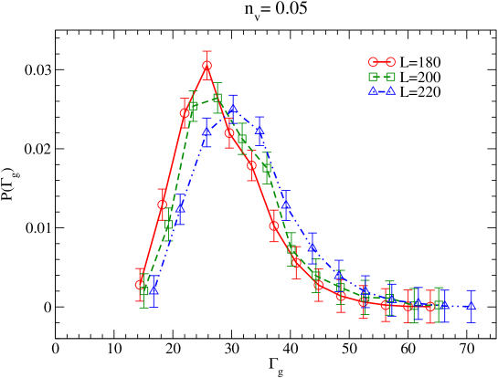
Figure 10: Histogram of $\Gamma_{g}$, corresponding to the lowest nonzero gap for the three largest sizes studied at $n_{v}=0.05$.

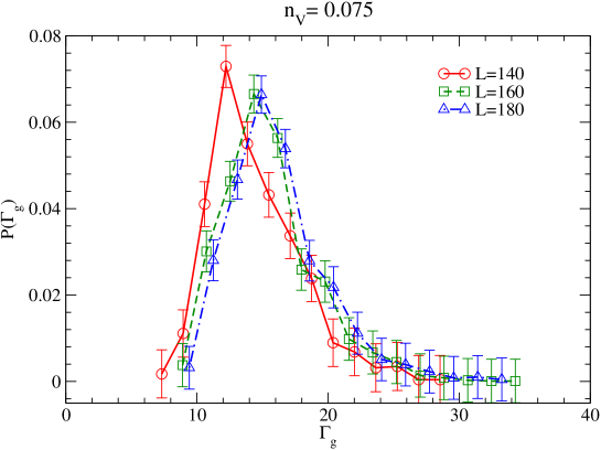
Figure 11: Histogram of $\Gamma_{g}$, corresponding to the lowest nonzero gap for the three largest sizes studied at $n_{v}=0.075$.

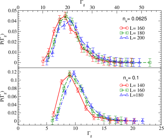
Figure 12: Histograms of $\Gamma_{\rm g}$ at the three largest values of $L$ studied for $n_{v}=0.0625$ and $n_{v}=0.1$.

Figure 7 displays $N_{L}(\Gamma)$ for $n_{v}=0.05$, for the three largest sizes studied. The corresponding extrapolation to the thermodynamic limit is shown in Fig. 8. The corresponding results for $n_{v}=0.075$ are displayed in Fig. 9. In all these figures, we focus on $\Gamma<\Gamma_{g}^{*}(L_{\rm min})$, where $L_{\rm min}$ is the smallest size for which data is displayed, and $\Gamma_{g}^{*}$ is read off from the peak in the histograms of $\Gamma_{g}$ shown in Fig. 10 and Fig. 11. The corresponding histograms for $n_{v}=0.0625$ and $n_{v}=0.1$ are displayed in Fig. 12

As is clear from these results for $n_{v}=0.05$ and $n_{v}=0.075$, $N_{L}(\Gamma)$ is found to fit well to a power-law form $N_{\rm 1D}\equiv c\Gamma^{-y}$ up to a fairly well-defined and readily-identified crossover scale $\Gamma_{c}(L)\equiv\log_{10}(t/|\epsilon_{c}(L)|)$. However, beyond $\Gamma_{c}$, the asymptotic fall-off is clearly faster than a power law. While the increase of $\Gamma_{c}(L)$ with $L$ is more significant at the smallest concentration studied ($n_{v}=0.05$), it is nevertheless clear that $\Gamma_{c}(L)$ does saturate to a finite value even in this case. This is clear from the fact that the extrapolated thermodynamic density of states $N(\Gamma)$ (Fig. 8) also displays the same crossover seen in the finite-size data. In the large-$\Gamma$ regime beyond this crossover, the modified Gade-Wegner form $N_{GW}(\Gamma)\equiv a\Gamma^{1/3}e^{-b\Gamma^{2/3}}$ is seen to provide a very good fit of the data for both these concentrations. The corresponding values of $\Gamma_{c}(L)$ and $\Gamma_{c}$, and of the best fit values of $y$, provide us additional points that fill in the curves shown in Fig. 4 and Fig. 6 of the main text, which display the $n_{v}$ dependence of $y$ and $\Gamma_{c}$, and the close relationship between $l_{c}\equiv N(\Gamma_{c})^{-1/2}$ and $l_{w}\equiv w^{-1/2}$. Finally, we re-emphasize a point made already in the main text: Our computational constraints prevent us from accessing the thermodynamic limit for the much larger values of $\Gamma$ at which we expect to see the same crossover for the lowest concentration $n_{v}=0.02$.

B.2 Extrapolations

Since states at any finite $\Gamma$ (i.e., away from the band center $\epsilon=0$) in such particle-hole symmetric hopping problems are not critical, one expects the leading corrections to the thermodynamic limit $N(\Gamma)$ at any finite $\Gamma$ to be regular rather than singular, similar to the finite-size corrections expected in noncritical phases of matter (i.e., away from critical points or critical lines). Guided by this rationale, the thermodynamic limit $N(\Gamma)$ is obtained from $N_{L}(\Gamma)$ by performing a polynomial extrapolation in $1/L$ (note that we expect that the leading finite-size corrections are ${\mathcal{O}}(1/L)$ rather than $\sim\exp(-L/\xi)$ because of “surface” contributions associated with the semi-open boundary conditions we employ). Since we are careful to only use large enough sizes for which almost every sample has at least one zero mode ($f_{L}\approx 1$), our finite-size data is already rather close to the thermodynamic limit, leading to a rather small secular drift with increasing $L$. In most cases, given the size of our error bars relative to the magnitude of this secular drift with $L$, the inclusion of the next-order term $c/L^{2}$ only results in an over-interpretation of statistical fluctuations. Therefore, a simple linear (in $1/L$) extrapolation $a+b/L$ has been used in most cases.

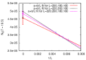
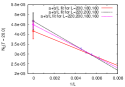
Figure 26: Comparison of thermodynamic limit of $N_{L}(\Gamma)$ at $n_{v}=0.0625$, taken with and without data at a larger size. At $n_{v}=0.0625$, the estimated value of $\Gamma_{c}$ is $\Gamma_{c}\approx 7$. Note that some correlation in the relative ordering of the three extrapolated values is expected over short intervals of $\Gamma$ since these data are correlated (obtained from the same set of random samples). However, over the range of $\Gamma$ from $\Gamma=7$ to $\Gamma=18$, we already see that there is no consistent ordering of the three extrapolated values, i.e., the red points are not always higher than the black points or vice-versa. Additionally, the three different extrapolations fall within (or lie at the edge of) each other’s error bars. Also, the results quoted in the main text (values of $\Gamma_{c}$ and $y$ in fits to $N_{\rm 1D}$ and the quality of the different fits) do not change significantly if our analysis is performed on the thermodynamic limit $N(\Gamma)$ obtained by including data at the larger size. All this, taken together, provides compelling evidence that our extrapolations to the thermodynamic limit are reliable.

We have also tested the stability of this extrapolation procedure to the inclusion of data at larger sizes. For the representative case of $n_{v}=0.0625$, this is shown Fig. 13, which is devoted to a comparison of the thermodynamic limit obtained in the main text using sizes $L=200,180,160$ with two other alternatives: A linear extrapolation from three sizes $L=220,200,180$, and a linear extrapolation from four sizes $L=220,200,180,160$. As is clear from this figure, all three extrapolations (i.e., the one used in the main text as well as the other alternatives which use data at a larger size) yield extrapolated values that lie within the error-bars of each other. Further, there is no systematic trend that suggests that any one of these extrapolations yields a consistently higher or lower value of $N(\Gamma)$ at all $\Gamma$. Details of all three extrapolations, for each value of $\Gamma$, are also shown as a separate multi-page figure (Fig. 26) placed at the end of this supplemental section for ease of inspection. Some examples of extrapolations used to arrive at $N(\Gamma)$ from data for $N_{L}(\Gamma)$ at other concentrations are also shown in Figs. 14, 15, 16, and 17. From this careful and detailed study, we conclude that our approach indeed allows us to reliably obtain the thermodynamic limit curve $N(\Gamma)$.

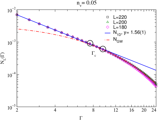
Figure 7: $N_{L}(\Gamma)$ at the three largest values of $L$ studied for $n_{v}=0.05$. Circles demarcate the crossover region centered at the crossover scale $\Gamma_{c}$. Data for $\Gamma\lesssim\Gamma_{c}$ fits well to power-law form $N_{\rm 1D}(\Gamma)$ (see text for details) with the value of $y$ indicated in the figure, while the large-$\Gamma$ regime fits well to the modified Gade-Wegner form $N_{\rm GW}(\Gamma)$.

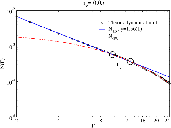
Figure 8: $N(\Gamma)$, the extrapolation to the thermodynamic limit of the finite-size data from the previous figure. Again, circles demarcate the crossover region centered at the crossover scale $\Gamma_{c}$. Data for $\Gamma\lesssim\Gamma_{c}$ fits well to power-law form $N_{\rm 1D}(\Gamma)$ with the value of $y$ indicated in the figure, while the large-$\Gamma$ regime fits well to the modified Gade-Wegner form $N_{\rm GW}(\Gamma)$.

Figure 9: $N_{L}(\Gamma)$ at the three largest values of $L$ studied for $n_{v}=0.075$. Circles demarcate the crossover region centered at the crossover scale $\Gamma_{c}$. Data for $\Gamma\lesssim\Gamma_{c}$ fits well to power-law form $N_{\rm 1D}(\Gamma)$ with the value of $y$ indicated in the figure, while the large-$\Gamma$ regime fits well to the modified Gade-Wegner form $N_{\rm GW}(\Gamma)$. Inset shows the extrapolation to the thermodynamic limit, in which the same crossover is clearly visible.

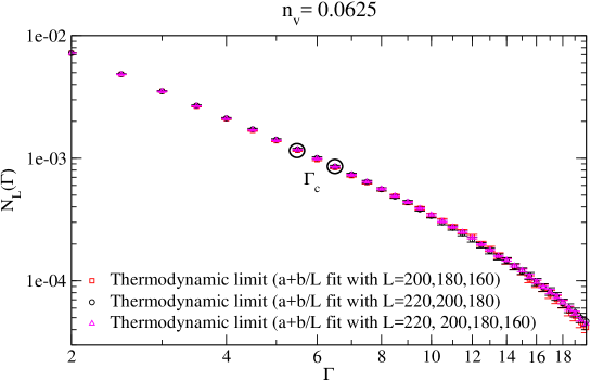
Figure 13: Three different extrapolations yield results for the thermodynamic limit $N(\Gamma)$ that fall within the error bars of each other, confirming the reliability and stability of our procedure to obtain the thermodynamic limit for the representative case of $n_{v}=0.0625$.

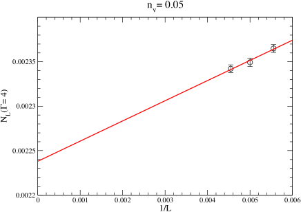
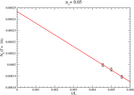
Figure 14: Examples of extrapolation of $N_{L}(\Gamma)$ to the thermodynamic limit at $n_{v}=0.05$. For this concentration, $\Gamma_{c}\approx 11$ (see Fig. 4 in the main text), and the left panel illustrates the extrapolation for $\Gamma<\Gamma_{c}$, while the right panel is for $\Gamma>\Gamma_{c}$. Note in particular that our extrapolation for $\Gamma>\Gamma_{c}$ is very likely an overstimate, so one can be fairly confident that $N(\Gamma)$ in the thermodynamic limit drops below $N_{1D}(\Gamma)$, ruling out a fit to this form for $\Gamma>\Gamma_{c}$.

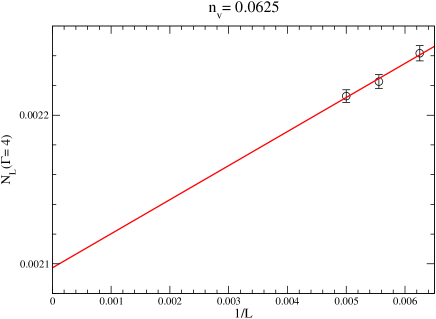
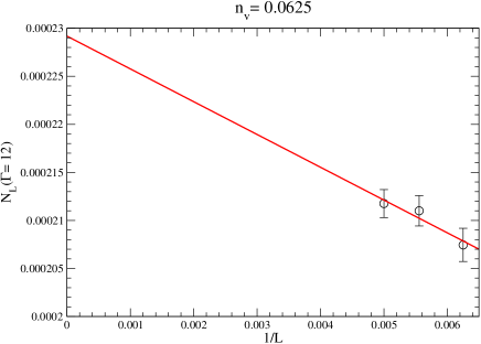
Figure 15: Examples of extrapolation of $N_{L}(\Gamma)$ to the thermodynamic limit at $n_{v}=0.0625$. For this concentration, $\Gamma_{c}\approx 7$ (see Fig. 4 in the main text), and the left panel illustrates the extrapolation for $\Gamma<\Gamma_{c}$, while the right panel is for $\Gamma>\Gamma_{c}$. Note in particular that our extrapolation for $\Gamma>\Gamma_{c}$ is very likely an overstimate, so one can be fairly confident that $N(\Gamma)$ in the thermodynamic limit drops below $N_{1D}(\Gamma)$, ruling out a fit to this form for $\Gamma>\Gamma_{c}$. Extrapolations at other values of $\Gamma$, as well as extrapolations including a larger size ($L=220$) are shown in Fig. 26.

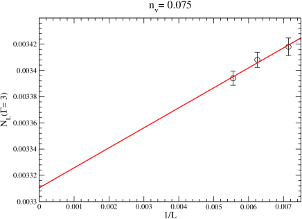
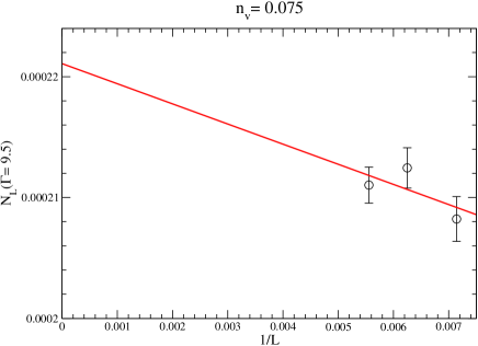
Figure 16: Examples of extrapolation of $N_{L}(\Gamma)$ to the thermodynamic limit at $n_{v}=0.075$. For this concentration, $\Gamma_{c}\approx 5$ (see Fig. 4 in the main text), and the left panel illustrates the extrapolation for $\Gamma<\Gamma_{c}$, while the right panel is for $\Gamma>\Gamma_{c}$. Note in particular that our extrapolation for $\Gamma>\Gamma_{c}$ is very likely an overstimate, so one can be fairly confident that $N(\Gamma)$ in the thermodynamic limit drops below $N_{1D}(\Gamma)$, ruling out a fit to this form for $\Gamma>\Gamma_{c}$.

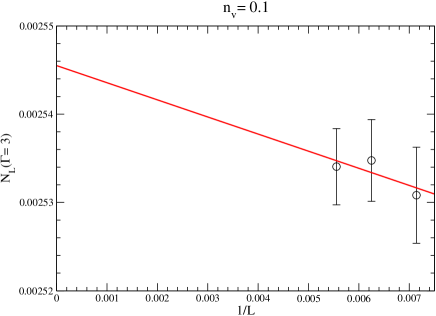
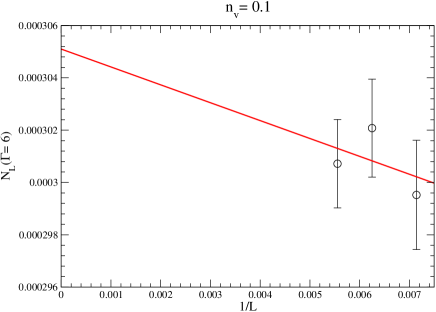
Figure 17: Examples of extrapolation of $N_{L}(\Gamma)$ to the thermodynamic limit at $n_{v}=0.1$. For this concentration, $\Gamma_{c}\approx 4$ (see Fig. 4 in the main text), and the left panel illustrates the extrapolation for $\Gamma<\Gamma_{c}$, while the right panel is for $\Gamma>\Gamma_{c}$. Note in particular that our extrapolation for $\Gamma>\Gamma_{c}$ is very likely an overstimate, so one can be fairly confident that $N(\Gamma)$ in the thermodynamic limit drops below $N_{1D}(\Gamma)$, ruling out a fit to this form for $\Gamma>\Gamma_{c}$.

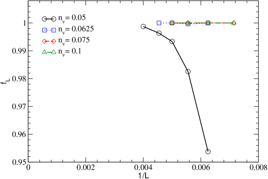
Figure 18: Probability $f_{L}$ that an $L\times L$ sample has at least one pair of zero modes tends to $1$ in the thermodynamic limit for each concentration studied. Due to our computational constraints, we have been unable to obtain such data at $n_{v}=0.02$, where we expect the density of zero modes to be much lower, but $f_{L}$ to still tend to $1$ in the thermodynamic limit (based on the analytical arguments given in the main text).

Appendix C Further analysis of zero modes

Our data for $f_{L}$, the probability that an $L\times L$ sample has at least one zero mode, is shown in Fig. 18. Clearly, $f_{L}$ tends to $1$ as $L\rightarrow\infty$, as already mentioned in the main text. This is consistent with the analytical argument in the main text, which also provides a simple rigorous lower bound for the density of zero modes. The 4-triangle zero mode used in this argument is the first term in an infinite series in $n_{v}$, with higher powers of $n_{v}$ arising from bigger patterns consisting of a larger number of impurities in specific locations relative to each other. In Fig. 19 and Fig. 20, we show a few examples of zero mode constructions that contribute to this series. However, as already noted in the main text, terms in this series do not give the dominant contribution to $w$ at the not-too-small values of $n_{v}$ studied by us in this work. Indeed, we have explicitly measured the density of 4-triangles and checked that it is significantly smaller than the density of zero modes for all $n_{v}$ at which we have computed $w$ (including $n_{v}=0.05$). Additionally, we have enumerated all possible clusters of fewer than four impurities and verified that it is not possible to produce a similar zero mode with fewer than four vacancies in a cluster so long as the exclusion constraints outlined in the main text are in place.

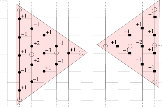
Figure 19: Two kinds of 5-vacancy clusters (“5-triangles”) that host an exact zero mode, with the corresponding wavefunction marked. Open circles correspond to vacancies.

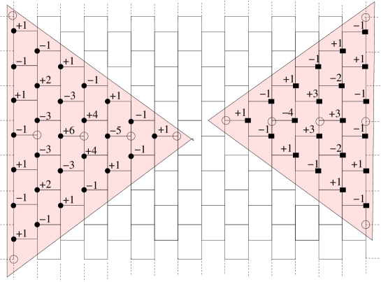
Figure 20: Two kinds of 6-vacancy clusters (“6-triangles”) that host an exact zero mode, with the corresponding wavefunction marked. Open circles correspond to vacancies.

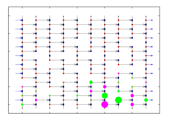
Figure 21: An $L\times L$ semi-open sample (of the type consistently used in all our numerical work) with $L=10$, with vacancies represented by missing lattice sites. This sample provides a simple example of a zero mode that does not seem to arise from any of the regular arrangements of vacancies used in our zero mode constructions. The actual wavefunction of this zero mode is represented by color-coded circles. The size of the circle corresponds to the magnitude of the wavefunction at the corresponding site, while the two different colors represent opposite signs for the wavefunction at the corresponding sites.

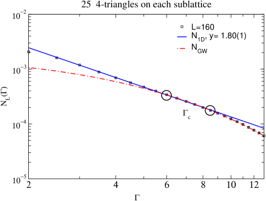
Figure 22: $N_{L}(\Gamma)$ in the toy model in which a $L=160$ sample is diluted with $25$ randomly placed 4-triangles on each sublattice. Circles demarcate the crossover region centered at the crossover scale $\Gamma_{c}$. Data for $\Gamma\lesssim\Gamma_{c}$ fits well to power-law form $N_{\rm 1D}(\Gamma)$ with the value of $y$ indicated in the figure, while the large-$\Gamma$ regime fits well to the modified Gade-Wegner form $N_{\rm GW}(\Gamma)$.

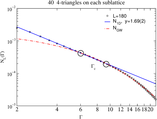
Figure 23: $N_{L}(\Gamma)$ in the toy model in which a $L=180$ sample is diluted with $40$ randomly placed 4-triangles on each sublattice. Circles demarcate the crossover region centered at the crossover scale $\Gamma_{c}$. Data for $\Gamma\lesssim\Gamma_{c}$ fits well to power-law form $N_{\rm 1D}(\Gamma)$ with the value of $y$ indicated in the figure, while the large-$\Gamma$ regime fits well to the modified Gade-Wegner form $N_{\rm GW}(\Gamma)$.

The zero mode associated with the ${\mathcal{R}}_{6}$ motif described in the main text also generalizes in an obvious way to yield a series of zero modes that all survive the effects of bond disorder in a manner completely analogous to the ${\mathcal{R}}_{6}$ zero mode. These ${\mathcal{R}}_{n}$ zero modes ($n>6$) live on larger and larger equilaterial triangles (with zig-zag edges) which are connected to the rest of the lattice only via $B$ ($A$) sublattice sites but have more undeleted $A$ ($B$) sublattice sites than $B$ ($A$) sublattice sites, allowing a zero mode to exist within the triangle for generic realizations of bond-disorder. As in the case of the ${\mathcal{R}}_{6}$ zero mode described in the main text, this robustness to disorder follows from the fact that the number of free components of the wavefunction of any such mode is one more than the number of zero-energy equations that they must satisfy.

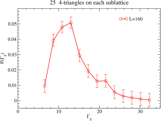
Figure 24: Histogram of $\Gamma_{g}$, corresponding to the lowest nonzero gap for the $L=160$ sample diluted with $25$ randomly placed 4-triangles on each sublattice.

We have also found other simple examples of such “${\mathcal{R}}$-type” zero modes that live near the armchair boundary and are not associated with a specific regular arrangement of vacancies. Instead, as already mentioned earlier, these modes appear to generically live in a region ${\mathcal{R}}$ which connects to the rest of the lattice only via $B$ ($A$) sublattice sites belonging to ${\mathcal{R}}$, although it has more undeleted $A$ ($B$) sublattice sites than $B$ ($A$) sublattice sites. In such a region, $T_{AB}T^{\dagger}_{AB}$ ($T^{\dagger}_{AB}T_{AB}$) has a zero mode living on the $A$ ($B$) sublattice sites, simply because the number of constraints that need to be satisfied by this zero mode wavefunction is smaller than the number of $A$ ($B$) sublattice sites on which this zero mode lives. As already noted, this feature also guarantees that such zero modes survive the effects of disorder in the nearest-neighbour hopping amplitudes. One example of such a mode is shown in Fig. 21. We believe that bulk versions of such more general ${\mathcal{R}}$-type zero modes provide the dominant contribution to $w$ for the values of $n_{v}$ studied by us, which is why our lower-bound on $w$ (obtained by thinking in terms of Fig. 2 in the main text) substantially underestimates $w$ at such not-too-small values of $n_{v}$. Clearly, no additional local correlations among impurities can entirely eliminate such more general ${\mathcal{R}}$-type zero modes . Therefore, a non-zero density of zero-energy modes is expected to be a generic feature of such systems. However, we have been unable to convert this observation into an improved lower-bound.

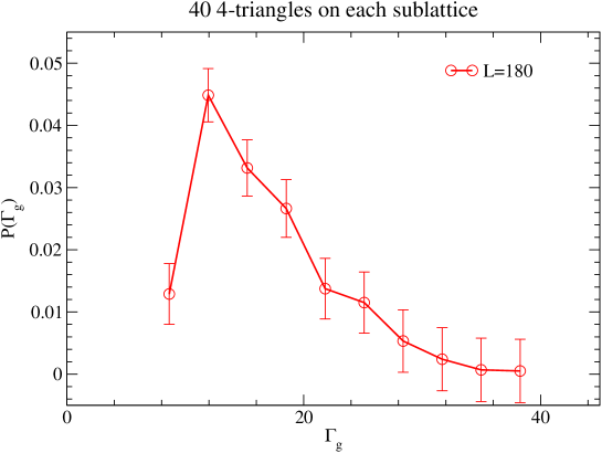
Figure 25: Histogram of $\Gamma_{g}$, corresponding to the lowest nonzero gap for the $L=180$ sample diluted with $40$ randomly placed 4-triangles on each sublattice.

Appendix D Dilution by 4-triangles

Finally, we provide an illustration of the importance of spatial correlations between vacancies via a simple toy model in which vacancies enter the sample only in groups of four, arranged as a 4-triangle at random locations in the sample (as in Fig. 3 of the main text). In Figs. 22 and 23, we respectively display the density of states of $L\times L$ samples with $L=160$ and $L=180$. The $L=160$ sample is diluted by $25$ 4-triangles placed at random on each sublattice, while the $L=180$ sample is diluted with $40$ 4-triangles placed at random on each sublattice. The former sample corresponds to a “bare” value of $n_{v}\approx 0.0039$, while the latter sample corresponds to a bare value of $n_{v}\approx 0.0049$. These values of $n_{v}$ are an order of magnitude different from the values of $n_{v}$ studied by us in the main part of our work (in which the impurities are uncorrelated except for exclusion constraints designed to prevent the occurrence of “trivial” zero modes). However, since all vacancies go in as part of a 4-triangle, $w\approx 9.76\times 10^{-4}$ for the $L=160$ sample and $w\approx 1.23\times 10^{-3}$ for the $L=180$ sample. The values of $w$ are thus very similar to those obtained in our independently diluted samples with $n_{v}$ in the range $0.05$—$0.06$.

From Figs. 22 and 23, we see that the density of states again undergoes a crossover that is qualitatively the same as the crossover identified in our main study. However, the corresponding $\Gamma_{c}$ is much smaller (i.e., the energy scale $|\epsilon_{c}|$ is much larger) than one would have expected based on the value of the overall vacancy concentration $n_{v}$ (had the vacancies been independent as in the main study). Similarly, the value of $y$ is also very different from the (extrapolated) value of $y$ one would have expected at such small $n_{v}$. The corresponding histograms of $\Gamma_{g}$ are shown in Figs. 24 and 25. From these figures, we see that $\Gamma_{g}^{*}$, corresponding to the position of the peak in the histogram of $\Gamma_{g}$, is significantly smaller than one would have expected based on the overall vacancy concentration $n_{v}$ (had the vacancies been independent, as in the main study). This provides a simple illustration of the importance of spatial correlations between vacancies in setting the lowest gap scale $\Gamma_{g}^{*}$, and the density of zero modes $w$. It also emphasizes that the crossover identified by us is a robust and generic aspect of the low-energy physics of vacancy-disorder.

Finally, we note that the values of $\Gamma_{c}$ and $y$ in the case of dilution by 4-triangles are apparently predicted much better by the value of $w$ (as opposed to the $n_{v}$). This raises the interesting questions already alluded to in the main text: Are $\Gamma_{c}$ and $y$ determined in a “universal” way (i.e., independent of short-ranged correlations between vacancies and other such microscopic details) by the value of the zero-mode density $w$ in the limit of small but nonzero $w$? Can this dependence be understood in terms of a low-energy effective theory or renormalization group approach?

References

- (1) P. A. Lee and T. V. Ramakrishnan, Rev. Mod. Phys. 57, 287 (1985).
- (2) A. Altland, B. D. Simons, and M. R. Zirnbauer, Phys. Rep. 359, 283 (2002).
- (3) F. Evers and A. D. Mirlin, Rev. Mod. Phys. 80, 1355 (2008).
- (4) R. Gade, Nucl. Phys. B 398, 499 (1993).
- (5) R. Gade and F. Wegner, Nucl. Phys. B 360, 213 (1991).
- (6) O. I. Motrunich, K. Damle, and D. A. Huse, Phys. Rev. B 65, 064206 (2002).
- (7) P. T. Araujo, M. Terrones, M. S. Dresselhaus, Materials Today 15, 98 (2012).
- (8) G. Forte, A. Grassi, G. M. Lombardo, A. La Magna, G. G. N. Angilella, R. Pucci, R. Vilardi, Phys. Lett. A 372, 6168 (2008).
- (9) V. M. Pereira, J. M. B. Lopes dos Santos, and A. H. Castro Neto, Phys. Rev. B 77, 115109 (2008).
- (10) V. M. Pereira, F. Guinea, J. M. B. Lopes dos Santos, N. M. R. Peres, and A. H. Castro Neto, Phys. Rev. Lett. 96, 036801 (2006).
- (11) T. O. Wehling, S. Yuan, A. I. Lichtenstein, A. K. Geim, and M. I. Katsnelson, Phys. Rev. Lett. 105, 056802 (2010).
- (12) F. J. Dyson, Phys. Rev. 92, 1331 (1953).
- (13) G. Theodorou and M. H. Cohen, Phys. Rev. B 13, 4597 (1976).
- (14) T. P. Eggarter and R. Riedinger, Phys. Rev. B 18, 569 (1978).
- (15) O. Motrunich, K. Damle, and D. A. Huse, Phys. Rev. B 63, 134424 (2001).
- (16) O. Motrunich, K. Damle, and D. A. Huse Phys. Rev. B 63, 224204 (2001).
- (17) I. A. Gruzberg, N. Read, and S. Vishveshwara, Phys. Rev. B 71, 245124 (2005).
- (18) P. W. Brouwer, A. Furusaki, I. A. Gruzberg, and C. Mudry, Phys. Rev. Lett. 85, 1064 (2000).
- (19) P. W. Brouwer, C. Mudry, and A. Furusaki, Phys. Rev. Lett. 84, 2913 (2000).
- (20) M. Titov, P. W. Brouwer, A. Furusaki, and C. Mudry, Phys. Rev. B 63, 235318 (2001).
- (21) C. Mudry, S. Ryu, A. Furusaki, Phys. Rev. B 67, 064202 (2003).
- (22) A. J. Willans, J. T. Chalker, and R. Moessner, Phys. Rev. B 84, 115146 (2011)
- (23) V. Hafner, J. Schindler, N. Weik, T. Mayer, S. Balakrishnan, R. Narayanan, S. Bera, and F. Evers, Phys. Rev. Lett. 113, 186802 (2014).
- (24) P. M. Ostrovsky, I. V. Protopopov, E. J. Konig, I. V. Gornyi, A. D. Mirlin, and M. A. Skvortsov, Phys. Rev. Lett. 113, 186803 (2014).
- (25) E. H. Lieb and M. Loss, Duke Math. J. 71, 337 (1993).
- (26) S. Ryu and Y. Hatsugai, Phys. Rev. Lett. 89, 077002 (2002).
- (27) L. Brey and H. A. Fertig, Phys. Rev. B 73, 235411 (2006).
- (28) P. W. Brouwer, E. Racine, A. Furusaki, Y. Hatsugai, Y. Morita, and C. Mudry, Phys. Rev. B 66, 014204 (2002).
- (29) https://en.wikipedia.org/wiki/ALGOL
- (30) R. S. Martin and J. H. Wilkinson in Handbook for Automatic Computation, Vol. II: Linear Algebra, J. H. Wilkinson and C. Reinsch (eds.), Springer-Verlag (Berlin, 1971).
- (31) S. Sanyal, Ph.D thesis, Tata Institute of Fundamental Research, Mumbai, 2014, http://theory.tifr.res.in/Research/Thesis/
- (32) https://en.wikipedia.org/wiki/ GNU_Multiple_Precision_Arithmetic_Library
- (33) https://en.wikipedia.org/wiki/LAPACK