Differences in Halo-Scale Environments between Type 1 and Type 2 AGNs at Low Redshift

Abstract

Using low-redshift ($z<0.09$) samples of AGNs, normal galaxies and groups of galaxies selected from the Sloan Digital Sky Survey (SDSS), we study the environments of type 1 and type 2 AGNs both on small and large scales. Comparisons are made for galaxy samples matched in redshift, $r$-band luminosity, [O III] luminosity, and also the position in groups (central or satellite). We find that type 2 AGNs and normal galaxies reside in similar environments. Type 1 and type 2 AGNs have similar clustering properties on large scales ($\gtrsim 1~{}\,h^{-1}{\rm{Mpc}}$), but at scales smaller than $100\,h^{-1}{\rm{kpc}}$, type 2s have significant more neighbors than type 1s ($3.09\pm 0.69$ times more for central AGNs at $\lesssim 30\,h^{-1}{\rm{kpc}}$). These results suggest that type 1 and type 2 AGNs are hosted by halos of similar masses, as is also seen directly from the mass distributions of their host groups ($\sim 10^{12}h^{-1}\,M_{\odot}$ for centrals and $\sim 10^{13}h^{-1}\,M_{\odot}$ for satellites). Type 2s have significantly more satellites around them, and the distribution of their satellites is also more centrally concentrated. The host galaxies of both types of AGNs have similar optical properties, but their infrared colors are significantly different. Our results suggest that the simple unified model based solely on torus orientation is not sufficient, but that galaxy interactions in dark matter halos must have played an important role in the formation of the dust structure that obscures AGNs.

1. Introduction

It is widely believed that almost all massive galaxies have supermassive black holes (SMBHs) in their centers, and that active galactic nuclei (AGNs) are SMBHs actively accreting surrounding materials. Observationally, AGNs are classified into two populations, type 1 and type 2, depending on whether broad emission lines appear in their optical spectra. The most popular model hypothesizes that the two types are intrinsically the same, and the observed differences between the two are attributed solely to orientation effects (Antonucci 1993). In such a unified model, a type 1 AGN is assumed to be observed with a direct view of its nucleus, while the accretion disk and the broad-line region (BLR) of a type 2 AGN are blocked by an optically thick obscuring structure, called ’torus’. However, evidence has emerged that the simple unified model may not be able to explain all of the observational facts. Some revisions of the model, for example including the evolution of torus and the BLR (e.g., Laor 2003; Elitzur & Ho 2009; Gu et al. 2013; Elitzur et al. 2014), are needed (see the review by Netzer 2015 and references therein).

If type 1 and type 2 AGNs differed only in their orientations, they would be expected to have similar circumgalactic environments on halo and larger scales. The large scale environments of AGNs are usually measured by the auto-correlation function of AGNs (e.g., Porciani et al. 2004; Wake et al. 2004; Croom et al. 2005; Myers et al. 2007; Shen et al. 2007; Ross et al. 2009; Eftekharzadeh et al. 2015; Chehade et al. 2016), the cross-correlation function between AGNs and galaxies (e.g., Li e al. 2006; Coil et al. 2007; Hickox et al. 2009; Krumpe et al. 2010; Miyaji et al. 2011; Shen et al. 2013; Zhang et al. 2013; Shao et al. 2015), and their modifications (e.g., Dahari 1984; Schmitt 2001; Ellison et al. 2011; Kollatschny et al. 2012).

To test the unified model, some early studies have examined the environments of AGNs, using relatively small AGN samples (typically a few tens to $\sim 100$ AGNs). These studies have found that type 2 AGNs tend to have more close companions within $\sim 100\,h^{-1}{\rm{kpc}}$ than type 1s (e.g. Laurikainen & Salo 1995; Dultzin-Hacyan et al. 1999; Krongold et al. 2002; Koulouridis et al. 2006). Based on the cross correlation between a large sample of local AGNs and photometric galaxies, Strand et al. (2008) found a similar but weaker trend on larger scales , $\sim 2\,h^{-1}{\rm{Mpc}}$. In addition to the number of companions, Villarroel & Korn (2014) found that the color and activity are systematically different between the neighbors of type 1 and type 2 AGNs, and that the spiral fraction of the host galaxies depends on the environment of type 1 and type 2 AGNs in different ways. All these are at odds with the expectation of the simple unified model.

More studies based on high redshift AGNs (usually called quasars) have also been carried out to examine the unified model. Unlike local AGNs, high-$z$ type 2 AGNs are selected according to their high absorption column densities or strong dust extinctions, inferred from both X-ray and infrared (IR) data. Early results found no obvious difference between type 1 (unobscured) and type 2 (obscured) AGNs in their clustering, giving support to the unified model (e.g. Ebrero et al. 2009; Coil et al. 2009; Gilli et al. 2009; Geach et al. 2013). However, more recent studies suggested that the angular clustering amplitudes for the two types of AGNs are significantly different, with type 2s being more strongly clustered than type 1s (e.g. Hickox et al. 2011; Elyiv et al. 2012; Donoso et al. 2014; DiPompeo et al. 2014; but see Allevato et al. 2011, 2014 for some different results), consistent with the results obtained for local AGNs. Similar results were found by DiPompeo et al. (2015, 2016) using the cross correlation between the cosmic microwave background (CMB) lensing map and the distributions of the two AGN populations. All these studies suggest that type 2 AGNs tend to live in more massive halos. However the difference in the inferred halo masses vary greatly from study to study.

It should be emphasized, however, that many early investigations have already revealed that AGN clustering depends on various properties, such as the luminosity ($L_{\rm bol}$, e.g., Serber et al. 2006; Strand et al. 2008), redshift (e.g., Croom et al. 2005; Zhang et al. 2013; Eftekharzadeh et al. 2015) and various other attributes of the host galaxies (e.g. Li et al. 2006; Coil et al. 2009; Hickox et al 2009; Mandelbaum et al. 2009; Mendez et al. 2016; see also §2.3). If the samples of the type 1 and type 2 AGNs used in the clustering analyses have different distributions in these properties, the results obtained may be biased and, therefore, are difficult to be used to constrain theoretical models, such as the unified model.

In this paper, we analyze the environmental dependence of AGNs using a large, well-designed type 1 and type 2 AGN samples at low-redshift selected from the Sloan Digital Sky Survey (SDSS). These AGN samples have reliable measurements of AGN parameters and other information about the host galaxies. With all these, we can build well-defined and well-controlled samples for our analysis. Our primary goal is to compare the environments of the two types of AGNs on both small and large scales using cross-correlations between AGNs and reference galaxies. Compared with previous studies of quasar clustering, our low-redshift samples are much more suited to study environments on relatively small scales, because here galaxies that are used to trace the environments of AGNs can be observed to faint luminosities. We also use groups of galaxies to study the small scale environments of AGNs, double-checking the results obtained from the cross-correlation analysis. As we will show later, type 1 and type 2 AGNs reside in halos with similar mass distributions but have different number of galaxy companions within halos, which is inconsistent with the assumption that type 1 and type 2 AGNs differ only in orientation, and suggests a difference in physical mechanisms related to triggering, fueling and obscuration between the two types of AGNs. To better understand the origin of this difference, we also analyze the environments of matched normal (inactive) galaxies.

The paper is organized as follows. In Section 2 we introduce the data and samples used in this paper. In Section 3 we present our results concerning AGN environments, using cross-correlation between AGNs and normal galaxies. We analyze the properties of the host halos and host galaxies of different types of AGNs in Section 4. Finally, we summarize our results and discuss their implications in Section 5.

2. Data and Samples

The data used in this paper are primarily obtained from SDSS, using results previously obtained both by ourselves and others. To investigate the environments and hosts of AGNs, we need to construct samples not only for AGNs (both type 1 and type 2), but also for normal galaxies and for groups of galaxies.

2.1. The Parent AGN Samples

The parent AGN sample is selected from SDSS DR4 (Adelman-McCarthy et al. 2006). The AGN classification is based on the traditional definition that relies on the presence or absence of broad emission lines in the AGN optical spectra. In Dong et al. (2012), a set of elaborate, automated selection procedures was developed to conduct AGN–galaxy spectral decomposition and continuum/emission-line fitting. Dong et al. started with 451,000 spectra classified by the SDSS spectroscopic pipeline as ”galaxy” or ”QSO” at $z<0.35$ (to ensure that H$\alpha$ emission line is in the spectrum) in the SDSS DR4. Since H$\alpha$ emission is in general the strongest broad line in the optical spectra of AGNs, Seyfert 1s are identified according to the presence of broad H$\alpha$. The criteria of the reliable detection of broad H$\alpha$ are set quantitatively according to the prominence of broad-H$\alpha$ flux as well as the statistical significance (see Dong et al 2012 for the detail). This procedure yields a total of 8,862 broad-line AGNs at $z<0.35$ with secure detections of the broad H$\alpha$ line. These AGNs form the parent sample of type 1 AGNs adopted here.

The type 2 AGN sample is the one built by Dong et al. (2010). It comprises 27,306 Seyfert 2 galaxies in the SDSS DR4 selected in the BPT line-ratio diagram (Baldwin, Phillips & Terlevich 1981) using the demarcation lines of Kauffmann et al. (2003). All the narrow emission lines, H$\beta$, [O III] $\lambda 5007$, H$\alpha$ , and [N II] $\lambda 6583$ are required to be detected at $>5~{}\sigma$ significance. In order to measure the emission lines reliably, the following procedure is applied. First the starlight continuum, obtained from stellar templates broadened and shifted to match the stellar velocity dispersion of the galaxy in question, is subtracted to obtain a clean emission-line spectrum. Note that the stellar absorption features are thus subtracted, ensuring the reliable measurements of weak emission lines. Each emission line is fitted incrementally with as many Gaussians as statistically justified; basically, 2 Gaussians are used to model every doublet line of [O III] $\lambda\lambda 4959,5007$ and 1 Gaussian is sufficient to model the others. We refer the reader to Dong et al. (2010; their Section 2.2) for the details of the spectral fitting, sample construction, and measurements of the AGN properties. The broad-line objects in the type 1 sample of Dong et al (2012) are eliminated even if they are selected according to the above criteria.

2.2. Galaxies and Groups of Galaxies

The galaxy sample used here is the same as that used in Yang et al. (2007, hereafter Y07) in the construction of their galaxy group catalog. It is based primarily on the New York University Value-Added Galaxy Catalogue (NYU-VAGC; Blanton et al. 2005) of the SDSS DR7 (Abazajian et al. 2009). Y07 selected all galaxies in the main galaxy sample, with $r$-band Petrosian magnitudes $r\leq 17.77$ after correcting for Galactic extinction (Schlegel et al. 1998), with redshifts in the range $0.01\leqslant z\leqslant 0.2$, and with redshift completeness $C>0.7$. Among these galaxies, 599,301 have redshifts from the SDSS, 3,269 have redshifts taken from other redshift surveys, and 36,789 that lack redshifts due to fiber collisions have assigned redshifts of their nearest neighbors. It should be noted that, although this fiber collision correction works well in roughly 60% of all cases, the remaining 40% can be very different from their corresponding true values (Zehavi et al. 2002). In this paper, the sample of galaxies with redshift obtained from SDSS and other redshift surveys, as well as from fiber collision corrections is referred to as sample A, and the one including only measured redshifts (from both SDSS and other sources) is referred to as sample B.

From these galaxy samples, Y07 constructed galaxy group catalogs, using their halo-based group finder (Yang et al. 2005) and taking into account various observational selection effects. Each group is assigned a halo mass based on the ranking of its characteristic luminosity/stellar mass. Following the original definition, the brightest galaxy in a group is referred to as the central galaxy while all others as satellites. Unless specified otherwise, our results are presented for sample A and the group catalog constructed from it.

Figure 1.— The $L_{\rm[O\,{\footnotesize III}]}$ distributions of parent type 1 (blue) and type 2(red) samples at $z<0.09$. Dashed blue line is the distribution for type 1 AGNs that is scaled to have the same number as type 2s.

2.3. Control Samples of AGNs and Normal Galaxies

As noted above, each object in our parent type 1 AGN sample is identified either as a ”QSO” or as a ”galaxy” in the SDSS pipeline. Because of the redshift limit of our galaxy sample, many QSOs given by the SDSS pipeline do not lie in the volume within which galaxy groups are identified. In fact, the fraction of type 1 AGNs that are identified as galaxies by the SDSS pipeline is close to unity at $z<0.09$ and decreases gradually with redshift. In our analyses we will consider objects at $z\leq 0.09$ so that galaxies with $r$-band absolute magnitudes $M_{r}\leq-19.5$ are complete. In this redshift range, we have 1035 type 1 AGNs, about 94% of the objects selected into the parent sample.

As described in §2.1, the selection methods of type 1 and type 2 AGNs are different and thus the comparison as a whole should not be fair. Within the same redshift range ($z<0.09$), there are 12,621 type 2 AGNs, about 12 times as many as the type 1s. To carry out a fair comparison, a control sample of type 2 AGNs is constructed to match the properties of the type 1 sample. We choose to control four parameters: [O III] luminosity ($L_{\rm[O\,{\footnotesize III}]}$), $r$-band absolute magnitude ($M_{r}$), redshift ($z$) and central/satellite classification. The reasons for these are the following.

• $L_{\rm[O\,{\footnotesize III}]}$: Some previous studies have shown that AGN clustering properties depend on their $L_{\rm bol}$ (e.g., Li et al. 2006; Serber et al. 2006; Strand et al. 2008). On the other hand, it has been proposed that the covering factor of the torus may be directly related to $L_{\rm bol}$  as in the so called receding and approaching torus models (e.g., Lawrence 1991; Laor 2003; see also Netzer 2015 as a review). So a control in $L_{\rm bol}$ is needed to deal with the effects of any difference in $L_{\rm bol}$ between the type 1 and type 2 samples due to different torus covering factors. $L_{\rm[O\,{\footnotesize III}]}$ is commonly adopted as a good indicator of the $L_{\rm bol}$ of an AGN because it is believed to originate from the narrow line region and to be only weakly affected by the viewing angle relative to the torus (e.g., Heckman et al. 2004; Lamastra et al. 2009). As shown in Figure 1, the median of $L_{\rm[O\,{\footnotesize III}]}$ for type 1 AGNs in our sample is higher than that of type 2s by $\sim 0.8$ dex. To reduce any potential dependence on nuclear luminosity, we first match type 1 and type 2 samples in their $L_{\rm[O\,{\footnotesize III}]}$ distributions.

• $M_{r}$: It is well known that the clustering amplitude of galaxies depends significantly on galaxy luminosity, in that luminous galaxies tend to reside in more massive dark matter halos than fainter galaxies (e.g., White & Rees 1978; Yang et al. 2003; Vale & Ostriker 2004). Several recent studies have indeed suggested that AGN clustering, including the difference in clustering between obscured and unobscured AGNs, is simply determined by the luminosities of their host galaxies (e.g., Mendez et al. 2016). To avoid this effect, AGNs in our type 1 and type 2 samples are paired, so that the difference in the absolute magnitude between the two galaxies in each pair $|\Delta M_{r}|<0.1$.

• z: Redshift dependence of AGN clustering has been found in a number of previous studies (e.g., Croom et al. 2005; Zhang et al. 2013; Eftekharzadeh et al. 2015; Chehade et al. 2016). To minimize possible such dependence, the two samples are also paired in redshift, so that the redshift difference between the two AGN in a pair $\Delta z<0.01$.

• Central/satellite classification: This separation itself represents a characterization of the halo-scale environment and it has been known that central and satellite galaxies may evolve in different ways (e.g., Dressler 1980; Hashimoto et al. 1998). Among the type 1 AGNs in our working sample, about 79.4% are central galaxies according to the group catalog. The central fraction of type 2 AGNs is 79.1%, almost identical to that of type 1s. In matching type 1s and type 2s, centrals are only matched with centrals, and satellites only with satellites.

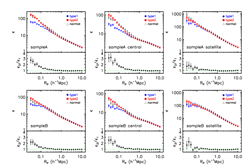
Figure 2.— In each panel, the top sub-panel shows the cross-correlations of control type 1 AGNs (red square), type 2 AGNs (blue circle) and normal galaxies (black triangle) with reference galaxies, and the bottom sub-panel shows the ratio of cross correlations between type 2 and 1 AGNs (black circle). The errors are given by bootstrap method as described in §3.1. The left panels show the results for all control AGNs and normal galaxies, the middle panels for central galaxies and right panels for satellites. The reference galaxies are constructed from sample A for the top three panels and sample B for the bottom panels. Please see Section 2 for the definitions of these samples.

In practice, for each type 1 AGN in our working sample, we select five type 2s with $|\Delta M_{r}|<0.1$ and $|\Delta z|<0.01$, which are in the same category (central or satellite) as, and have the $L_{\rm[O\,{\footnotesize III}]}$ closest to, the type 1 AGN in question. The measurements of $L_{\rm[O\,{\footnotesize III}]}$ are drawn directly from Dong et al. (2010, 2012). We choose five closest matches, instead of one, to reduce the statistical uncertainties. This is possible because we have many more type 2s than type 1s. The difference in $L_{\rm[O\,{\footnotesize III}]}$  between the matched pairs has a median value of zero and a variance $\sigma\sim 0.05$ dex. Finally we obtain type 1 and type 2 samples that have similar distributions in $L_{\rm[O\,{\footnotesize III}]}$, $M_{r}$, redshift and central/satellite fraction.

In addition to compare type 1 and type 2 AGNs, we also want to investigate the difference between active and normal galaxies so as to understand the environmental difference of AGNs and how AGNs are triggered and fueled. We will therefore also analyze the properties of a control sample of normal galaxies. For each AGN, a normal galaxy of the same category (central or satellite) is selected from the SDSS galaxy sample that has $M_{r}$ closest to that of the AGN in question and a redshift difference less than 0.01. Note that we do not eliminate active galactic nuclei from the pool of ”normal” galaxies in matching an AGN with another galaxy. Since AGNs are only a small fraction of all galaxies, including or excluding them in the matching pool does not make a difference. For each type 1 AGN in the working sample, five matches of normal galaxies are selected, while for each object in the control sample of type 2 AGNs, only one match is made. Our tests show that these two control samples give almost identical results for all the quantities examined in this paper. We therefore combine them into one control sample for normal galaxies, which is 10 times as large as the type 1 sample and 2 times as large as the control type 2 sample.

Table 1The Ratio of the Cross-Correlation between Type 2 and Type 1 AGNs ($\epsilon_{2}/\epsilon_{1}$)

Sample	$R_{P}=10^{-1.5}$	$R_{P}=0.1$	$R_{P}=10^{-0.5}$	$R_{P}=1$	$R_{P}=10^{0.5}$	$R_{P}=10$
(1)	(2)	(3)	(4)	(5)	(6)	(7)
$\rm sampleA(sA)$	$2.82\pm 0.89$	$1.56\pm 0.12$	$1.13\pm 0.04$	$0.98\pm 0.02$	$0.94\pm 0.02$	$0.95\pm 0.02$
$\rm sA~{}central$	$3.09\pm 0.69$	$1.75\pm 0.17$	$1.18\pm 0.06$	$1.02\pm 0.03$	$0.94\pm 0.02$	$0.95\pm 0.02$
$\rm sA~{}satellite$	$1.71\pm 0.70$	$1.42\pm 0.19$	$1.13\pm 0.06$	$0.96\pm 0.04$	$0.93\pm 0.03$	$1.00\pm 0.03$
$\rm sampleB(sB)$	$2.18\pm 0.53$	$1.33\pm 0.09$	$1.08\pm 0.04$	$0.97\pm 0.02$	$0.93\pm 0.02$	$0.95\pm 0.02$
$\rm sB~{}central$	$2.50\pm 0.63$	$1.44\pm 0.14$	$1.12\pm 0.06$	$1.01\pm 0.03$	$0.93\pm 0.02$	$0.95\pm 0.02$
$\rm sB~{}satellite$	$1.68\pm 0.61$	$1.27\pm 0.16$	$1.03\pm 0.06$	$0.93\pm 0.04$	$0.91\pm 0.03$	$1.00\pm 0.03$
$\rm sA~{}central^{1000}$	$2.80\pm 0.52$	$1.61\pm 0.13$	$1.16\pm 0.04$	$1.00\pm 0.01$	$0.93\pm 0.01$	$0.95\pm 0.01$

Note. — (1): The galaxy sample used to calculate the cross-correlation and for central/satellite division. Sample A refer to all galaxies with redshift obtained from SDSS and other redshift surveys, as well as from fiber collision corrections; sample B only include galaxies with spectroscopic redshift. The cross-correlation function $\epsilon$ is defined as formula 1. The last row is also for the sample A central AGNs, while adopting $v_{c}=1000$ $\mathrm{km~{}s^{-1}}$. (2)-(7): the $\epsilon_{2}/\epsilon_{1}$ with $R_{P}=10^{-1.5},0.1,10^{-0.5},1,10^{0.5},10~{}h^{-1}$ Mpc, respectively. Their errors are estimated from the bootstrap method.

2.4. Reference and Random Galaxy Samples

One of our goals is to quantify the environments in which different types of AGNs reside. Here we use galaxies as tracers of the environments. To this end, we use a reference sample of 170,095 galaxies with $M_{r}\leq-19.5$ at $z\leq 0.09$ in sample A. The magnitude cut is chosen to ensure that the reference sample is complete in the redshift range adopted for our control samples.

To account for the effects due to the irregular survey geometry, we also generate a random sample which is 200 times as large as the reference galaxy sample, with a total of 34,019,000 objects. The redshifts and magnitudes of these random galaxies are exactly the same as those in the reference sample, but with their coordinates (right ascension, declination) randomly selected from a uniform distribution in the sky. We determine whether or not a random galaxy is in the SDSS footprint, using the IDL program ‘is_in_windows.pro’ in idlutils. The geometry of the footprint is described by a set of polygons, and the areas around bright stars and sectors with ${\rm fgotmain}<0.7$ are excised.

3. Environments on Small and Large Scales

3.1. Cross-Correlation between AGNs and Galaxies

The cross-correlation between AGNs and galaxies has been used to analyze the environments of AGNs (e.g., Li et al. 2006, 2008; Hickox et al. 2009). Compared to the auto-correlation of AGNs, the cross-correlation is statistically more robust, because the large number of reference galaxies. More importantly, environments on small scales (e.g., ¡100 kpc) can only be studied by such cross-correlation analysis, because AGN pairs of such small separations are rare.

We define the cross-correlation function $\epsilon$ as,

$$\epsilon(R_{p})=\frac{N_{\rm R}}{N_{\rm G}}\frac{DG(r_{p}<R_{p},c\Delta z<v_{c})}{DR(r_{p}<R_{p},c\Delta z<v_{c})}\,,$$ (1)

where $\rm DG$ and $\rm DR$ are, respectively, the pair counts between AGNs and the reference (tracer) galaxies, and between AGNs and random galaxies, with projected separation $r_{p}<R_{p}$ and redshift difference $|c\Delta z|<v_{c}$; $N_{\rm G}$ and $N_{\rm R}$ are the total number of galaxies in the reference and random samples, respectively. Thus, if AGNs were randomly distributed with respect to galaxies, then $\epsilon=1$. We estimate the statistical errors in the cross-correlation measurements using the bootstrap method. To this end, we generate $N=1,000$ bootstrap AGN samples, each of which consists of AGNs randomly picked from original sample allowing multiple selections of individual objects. The pair counts, DG and DR, are estimated for each of the bootstrap sample, and their errors are given by the standard deviation of the measurements among all the bootstrap samples. It is interesting to note that the bootstrap error is almost identical to the Poisson error on small scales, because the total number of galaxies around each AGN is very low, and count of neighbors for individual AGNs is typically either 1 or 0. In our analyses, we choose $v_{c}=500~{}\mathrm{km~{}s^{-1}}$, motivated by the fact that it is about several times the virial velocity of a typical AGN host dark matter halo, which has a mass $\sim 10^{12}M_{\odot}$ (e.g., Padmanabhan et al. 2009; Ross et al. 2009; Shen et al. 2013; see also our results below). Our tests show that choosing an alternative value of $v_{c}=1000~{}\mathrm{km~{}s^{-1}}$ does not change our results significantly (see the last row of Table 1).

The cross-correlation results for type 1 and type 2 AGNs, together with their ratios ($\epsilon_{2}/\epsilon_{1}$), are presented in the top left panel of Figure 2. We also list the ratios and their bootstrap errors at a number of typical radii in Table 1. On large scales, the type 1 and control type 2 samples exhibit very similar clustering, implying that the two types of AGNs, on average, reside in halos of similar masses (see §4.1). On small scales, however, type 2 AGNs have much stronger clustering with galaxies than type 1s. At projected separation of $10^{-1.5}~{}\,h^{-1}{\rm{Mpc}}~{}(31.6~{}\,h^{-1}{\rm{kpc}})$, the average number of companions around type 2 AGNs is about $2.82\pm 0.89$ times that around type 1s. The $\epsilon_{2}/\epsilon_{1}$ decreases with increasing $R_{p}$, reaching a constant value of about one at $R_{p}>100\,\,h^{-1}{\rm{kpc}}$. This suggests that the spatial distribution of galaxies around type 2 AGNs is more concentrated than that around type 1s only on small scales, typically within the virial radii of the host halos of AGNs.

We also perform the same analyses for the control sample of normal galaxies (see also Figure 2). Their behavior looks similar to that the type 2 sample on both small and large scales, in good agreement with results obtained previously (see e.g. Li et al. 2008). This similarity in the clustering between type 2 AGNs and normal galaxies has been used to argue that the environments of AGNs are not very different from that of normal galaxies. However, our results show that this is true only for type 2 AGNs, but not for type 1s.

3.2. Centrals versus Satellites

According to current galaxy formation model (see e.g. Mo et al. 2010), central galaxies and satellite galaxies may have experienced different evolutionary processes. It is therefore interesting to analyze the central and satellite populations separately. In the middle and right panels of Figure 2, we show the cross correlations of central and satellite AGNs with the reference galaxies, respectively. For central galaxies, we again see that type 2 AGNs are more strongly clustered on small scales than type 1s, and that the two types have similar clustering amplitudes on large scales. However, the clustering difference on small scales is now more prominent than the total (central plus satellite) population. The ratio of the cross correlation function between type 2s and type 1s becomes larger than three at small project separations, and the signal extends to separations $\sim 200\,h^{-1}{\rm{kpc}}$. Here again the normal central galaxies have similar clustering amplitude as type 2 centrals on both large and small scales. In contrast, for satellites the difference between type 1 and type 2 is small and, indeed, insignificant given the error bars. Overall, satellites are more strongly clustered than centrals on both large and small scales, as is expected from the fact that they reside preferentially in more massive halos. These results demonstrate clearly that the difference in environment between type 1 and type 2 AGNs is mainly for the central population. Note that about 80% of all the AGNs in our samples are centrals. In what follows, we will focus on the central population.

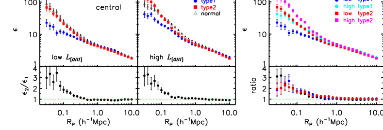
Figure 3.— Similar to Figure 2. The left (middle) panel shows the results for central AGNs of low (high) $L_{\rm[O\,{\footnotesize III}]}$ AGNs and their corresponding control normal galaxies. The right panel presents the results for total (low and high $L_{\rm[O\,{\footnotesize III}]}$) central AGNs. In the bottom sub-panel of right panel, the blue circles represent the ratio between high $L_{\rm[O\,{\footnotesize III}]}$ and low $L_{\rm[O\,{\footnotesize III}]}$ type 1 AGNs; and the red circles are the ratio between high $L_{\rm[O\,{\footnotesize III}]}$ and low $L_{\rm[O\,{\footnotesize III}]}$ type 2 AGNs. We also plot the ratio between type 2 and type 1 AGNs as the black circles for comparison.

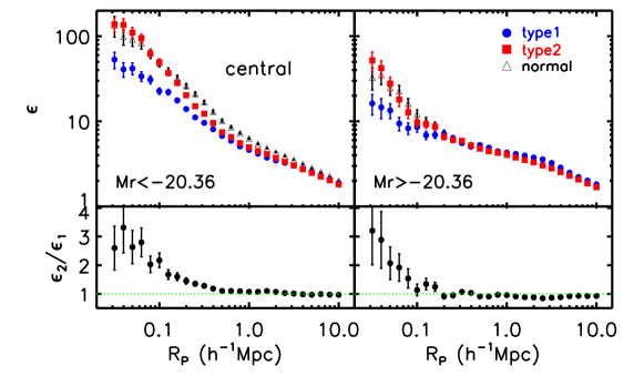
Figure 4.— Similar to Figure 2. The left and right panels show the results for high- and low-luminosity samples of central AGNs and their corresponding control normal galaxies, respectively.

3.3. Dependence on $L_{\rm[O\,{\footnotesize III}]}$

Environmental dependence of AGN luminosities has been investigated before (e.g. Serber et al. 2006; Strand et al. 2008). It is found that AGNs of higher luminosities tend to reside in denser environments. Here we investigate whether the difference in clustering properties between type 1 and type 2 AGNs also depends on AGN activities (as indicated by their $L_{\rm[O\,{\footnotesize III}]}$). To do this we divide each of the type 1 and 2 samples (only central galaxies) into two equal-sized subsamples according to the value of $L_{\rm[O\,{\footnotesize III}]}$. The median $L_{\rm[O\,{\footnotesize III}]}$ of the high-$L_{\rm[O\,{\footnotesize III}]}$ subsample is $\sim 0.7$ dex higher than the low-$L_{\rm[O\,{\footnotesize III}]}$ subsample. The cross correlation results of these subsamples are presented in Figure 3. The difference between the two types of AGNs on small scales is observed for both high- and low-$L_{\rm[O\,{\footnotesize III}]}$ samples, with type 2 AGNs having a higher cross correlation amplitude than type 1s. On large scales, the clustering amplitudes for the two types are quite similar, again suggesting similar host halo masses for both types. In the right panel, we plot the results for the high and low $L_{\rm[O\,{\footnotesize III}]}$ subsamples together. For a given type, the clustering amplitude increases significantly with $L_{\rm[O\,{\footnotesize III}]}$ at $R_{p}<200\,h^{-1}{\rm{kpc}}$ but no such increase is seen at larger separations. Such dependence is consistent with the results found in Strand et al. (2008).

3.4. High versus Low Galaxy Luminosity

In addition to the nuclear luminosity, the clustering amplitude of galaxies are also known to depend on galaxy luminosity, with intrinsically brighter galaxies having stronger clustering. It is therefore interesting to check whether or not the clustering difference between type 1 and type 2 AGNs also depends on the luminosities of host galaxies. To do this, we split each of our central AGN samples into two subsamples of equal size (in number) according to the $r$-band absolute magnitude ($M_{r}$) of the host galaxy. The cross correlation results for these subsamples are presented in Figure 4. Clearly, the difference on small scales ($<100\,h^{-1}{\rm{kpc}}$) and the similarity on large scales for the two types of AGNs are seen for both high and low luminosity subsamples. However, there are some noticeable differences in the results between the two subsamples. First, the clustering amplitude of the higher luminosity subsample is higher, consistent with the results of normal galaxies (e.g. Wang et al. 2007; Guo et al. 2010; Zehavi et al. 2011). Second, the clustering difference is noticeable only at $<100\,h^{-1}{\rm{kpc}}$ for the lower luminosity subsample, but extends to $\sim 300\,h^{-1}{\rm{kpc}}$ for the higher luminosity subsample. This may be understood if environmental effects that separate type 1 and type 2 AGNs operate on halo scales, because brighter galaxies reside preferentially in more massive galaxies which have larger virial radii. Finally, the cross correlations of normal galaxies in both of the luminosity ranges follow those of the corresponding type 2 subsamples.

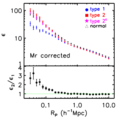
Figure 5.— Similar to Figure 2. In order to estimate the AGN contamination, for each of the type 1 AGNs, we remove the contribution of the AGN continuum to obtain a new $M_{r}$. Based on this corrected $M_{r}$, we construct new control samples of type 2 AGNs (type 2^c, magenta stars) and normal galaxies. For comparison, we also plot the results for the old sample of the type 2 AGNs (red square). The bottom panel shows the ratio between type 2^c and type 1 AGNs. Only results for central galaxies are presented.

3.5. Testing the Impact of Selection Effects

Is it possible that the clustering difference between type 1 and 2 AGNs on small scales is actually caused by some observational effects, rather than by real environmental effects? Because of fiber collisions, a few percent of the reference galaxies have no spectroscopic redshifts, and in Sample A they are assigned the redshifts of their nearest neighbors. As mentioned above, about 40% of the assigned redshifts are not reliable (Zehavi et al. 2002). In order to check whether or not such uncertainty is able to produce the clustering difference between type 1 and type 2 AGNs, we have repeated our analyses but using sample B, which only contains galaxies with spectroscopic redshifts. The results are shown in the bottom panels of Figure 2. As expected, the clustering amplitudes are reduced on small scales ($<100\,h^{-1}{\rm{kpc}}$) due to the elimination of close pairs by fiber collisions, but almost no change is seen on larger scales (see Li et al. 2006). However, the difference between type 1 and type 2 AGNs remains but is slightly reduced. The reduction is expected because type 2 AGNs, being more clustered with other galaxies on small scales, are more strongly affected by fiber collisions in their close pair counts.

Since the clustering strength is expected to depend on galaxy luminosity, the difference in the clustering may also be produced if the host galaxy luminosities of type 1 AGNs are systematically lower than those of type 2s. As an attempt to control this effect, we have matched their luminosity distributions in our control samples (see §2.3). However, the values of $M_{r}$ directly measured also include the contributions from AGNs themselves, and such contributions may be important for type 1 AGNs. To quantify the extent of AGN contamination in the observed luminosity, we define a parameter $\theta=f_{\rm AGN}/f_{\rm total}$, where $f_{\rm AGN}$ and $f_{\rm total}$ are the $r$-band flux of the AGN and the total flux, respectively. The $r$-band flux from the AGN is obtained by convolving the AGN component from our spectral decomposition (Dong et al. 2012) with the SDSS $r$-band filter throughput curves and $K$-correcting it to $z=0.1$. We found that $\theta$ for type 1 AGNs has a median value of $0.06$ and a maximum of about $0.45$. More than 90% of all the type 1 AGNs in our sample have $\theta<0.2$, consistent with the results obtained previously (e.g., Reines & Volonteri 2015), suggesting that any bias introduced is only moderate. This is also consistent with the fact that type 1 AGNs have very similar clustering properties on large scale to the corresponding control samples of normal galaxies that are matched in $M_{r}$. In order to test the effect more precisely, we construct a new control type 2 AGN sample and a normal galaxy sample, both matching the corrected $M_{r}$ distribution of the type 1 AGNs, with the AGN contributions to the luminosities subtracted. The new cross correlation results for the samples so matched, with matchings in other quantities the same as before, are presented in Figure 5. For comparison, the cross correlation for the old control sample of type 2 AGNs is also plotted. The results change little in the new matching, and the clustering difference on small scale ($<100\,h^{-1}{\rm{kpc}}$) is almost the same as before. We thus conclude that AGN contribution to the total galaxy luminosity is not the reason for the observed clustering difference between the two types of AGNs.

As shown above, the amplitude of AGN clustering increases with $L_{\rm[O\,{\footnotesize III}]}$. To take into account this effect, the control type 2 AGNs are matched in $L_{\rm[O\,{\footnotesize III}]}$with the type 1 sample. However, it may be possible that the torus can obscure the inner part of the [O III] emission line regions (e.g. Netzer et al. 2006; Zhang et al. 2008). This obscuration may be more important for type 2 AGNs, and so the intrinsic $L_{\rm[O\,{\footnotesize III}]}$ of type 2 AGNs may be systematically underestimated. If the extinction of [O III] is sufficient enough, the clustering difference between the two types of AGNs may be entirely due to dust extinction. Unfortunately, the extinction is hard to estimate. By comparing X-ray luminosity and mid-infrared line [O IV] luminosity with $L_{\rm[O\,{\footnotesize III}]}$, some earlier studies have suggested that the intrinsic $L_{\rm[O\,{\footnotesize III}]}$ of type 2 AGNs can on average be two times as high as the measured value (e.g., Netzer et al. 2006; Kraemer et al. 2011). However, if anisotropy in the X-ray emission is taken into account (e.g. Liu et al. 2014), the dust extinction may be much smaller. In Section 3.3, we have divided AGNs into high and low $L_{\rm[O\,{\footnotesize III}]}$ subsamples. The median $L_{\rm[O\,{\footnotesize III}]}$ of the high-$L_{\rm[O\,{\footnotesize III}]}$ subsample is $\sim 0.7$ dex higher than the low-$L_{\rm[O\,{\footnotesize III}]}$ subsample. The luminosity difference between the two subsamples is therefore much larger than the estimated extinction of $L_{\rm[O\,{\footnotesize III}]}$ for type 2 AGNs. The ratio of the cross correlations between the two subsamples is smaller than the ratio between type 1 and 2 AGNs (the right panel of Figure 3). Thus, even if $L_{\rm[O\,{\footnotesize III}]}$  of each of the type 2 AGNs is reduced by a factor of two by obscuration, the effect is still far too small to reproduce the difference between the two types of AGNs. Moreover, we also divide all type 2 AGNs into a sequence of subsamples with $L_{\rm[O\,{\footnotesize III}]}$ successively increased by a factor of 2 between adjacent subsamples. The clustering difference between adjacent subsamples are much smaller than that between the two types of AGNs. All these tests suggest that the underestimation of the intrinsic $L_{\rm[O\,{\footnotesize III}]}$ for type 2s cannot change our results significantly.

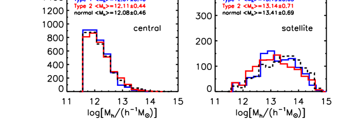
Figure 6.— Host halo mass distributions of type 1 (blue) and type 2 (red) AGNs. Results for normal galaxies (black) are also plotted for comparison. Left panel: central AGNs; Right panel: satellite AGNs. The data indicated in the panels are the medians and standard deviations of the distributions. For each type 1 AGN, five type 2 AGNs and ten normal galaxies are matched (see Section 2.3). To facilitate comparison, the distributions for type 1 AGNs and normal galaxies are scaled by a factor of 5 and 0.5, respectively.

4. Properties of Host Groups and Host Galaxies

The clustering difference indicates that the hosts of type 1 and type 2 AGNs may have different properties. Here we examine the properties of their hosts directly.

4.1. Properties of Host Halos

We use galaxy groups as given in Yang et al. (2007; see §2.2) to represent dark matter halos. We first compare the mass distributions of halos in which different types of AGNs reside (see Figure  6). We see that type 1 and type 2 AGNs have very similar halo mass distributions, consistent with the inference from their clustering properties on large scales. For central AGNs, both distributions peak around $10^{12}h^{-1}\,M_{\odot}$, in good agreement with results obtained previously for quasars (e.g. Richardson et al. 2012; Shen et al. 2009, 2013) and from galaxy groups (Pasquali et al. 2009). The halo masses of satellite AGNs are on average one order of magnitude higher than central AGNs, again consistent with the results of our clustering analyses. Note that the halo masses of the groups are estimated by ranking the total luminosity of member galaxies above a given luminosity, and some small halos are not assigned halo masses (see Y07 for more details). About $10\%$ of the central AGNs and $2\%$ of satellite AGNs in our samples do not have assigned halo masses. These systems, with halo masses all below $10^{11.6}h^{-1}M_{\odot}$ according to abundance matching, are not included in the plot.

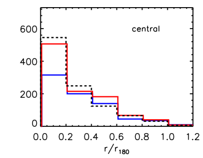
Figure 7.— The projected distance distribution of the closest satellites in the groups in which type 1 or 2 AGNs are central galaxies. The distance is normalized by the virial radius $r_{180}$. Similar to Fig. 6, the distributions for type 1 AGNs and normal galaxies are scaled by a factor of 5 and 0.5, respectively.

Next we check the number of satellite galaxies in the groups where AGNs are hosted by the central galaxies. On average, there are 347/822=0.42 satellites in each of the type 1 AGN group and 2089/4110=0.51 in each of the type 2 AGN groups. Here satellites with $M_{r}\leq-19.5$ and $M_{r}>-19.5$ are counted separately. If only bright satellites of $M_{r}<-19.5$ are used, the average numbers are 0.20 and 0.26 for type 1 and type 2, respectively. We have also examined the properties of these satellites, such as their $g-r$ color and Sérsic index, but no significant difference is found between halos hosting type 1 and type 2 AGNs.

The slopes of the cross-correlations on small scales suggest that the spatial distribution of galaxies around type 2 AGNs tend to be more centrally concentrated, in comparison to that around type 1 AGNs. To quantify this we measure the distribution of AGNs in terms of the projected distance each of them has to the closest satellite. Note again that almost all pairs ($\sim 97\%$) have $c|\Delta z|\leq 500\mathrm{km~{}s^{-1}}$. The distributions for different types of AGNs and normal galaxies are presented in Figure 7. To reduce the dependence on halo mass, the distance is normalized by the halo virial radius $r_{180}$ (see equation 5 in Y07). The distributions are not very different at $r/r_{180}>0.2$, although type 2s appear to have systematically more neighbors than type 1s up to $r/r_{180}\sim 1$. However, at $r/r_{180}<0.2$, the number of pairs for type 2 AGNs and normal galaxies are $\sim 1.7$ times that of type 1 AGNs. This clearly shows that type 2 AGNs on average have higher number of close pairs than type 1s.

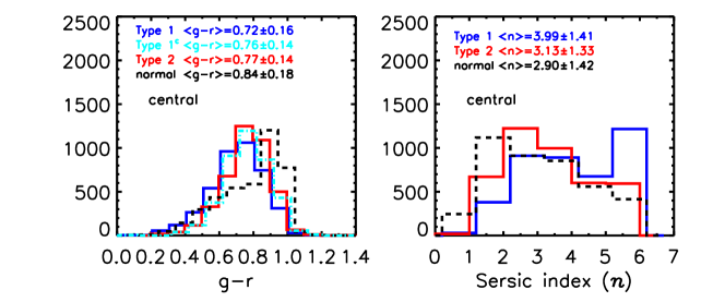
Figure 8.— The distributions of host galaxy properties for central type 1 (blue) and type 2 (red) AGNs, and normal galaxies (black). Left: $g-r$ color; right: Sérsic index. We also show the host galaxy color distribution after AGN continuum is subtracted for type 1 AGNs (cyan dot-dashed line). The numbers indicated in the panels are medians and standard deviations of the distributions. Similar to Fig. 6, the distributions for type 1 AGNs and normal galaxies are scaled by a factor of 5 and 0.5, respectively.

4.2. Properties of Host Galaxies

The $(g-r)$ color distributions of the host galaxies of the two types of AGNs as well as normal galaxies (only central galaxies) are shown in Figure 8. Type 1 AGNs on average are slightly bluer than type 2s. Since AGNs are blue and type 1 nuclei are more dominating in their hosts, the color difference seen between type 1 and type 2 AGNs might be produced by contaminations of the luminosities of the nuclei. To test this, we have re-calculated the $(g-r)$ colors of type 1 AGNs by subtracting the contributions of the nuclei from the total luminosities, using the method described in §3.5. We found that after this correction, the color difference between type 1 and type 2 AGNs becomes negligible. Both types of AGNs are bluer than normal galaxies. This is in agreement with the fact that AGNs are found to reside preferentially in the so-called “green valley” galaxies, with colors intermediate between star-forming blue cloud and the red sequence of galaxies (e.g., Nandra et al. 2007; Salim et al. 2007).

For reference, we also show the Sérsic index ($n$) distributions in the right panel of Figure 8. Type 1 AGNs show higher values of $n$, meaning that they have more concentrated light distribution. However, the high concentrations may be entirely due to the contributions of the relatively bright nuclei. In order to eliminate these contributions, careful image decompositions are needed.

The infrared color can also be used to study objects driven by different physical processes. We have cross matched galaxies in our working samples (central galaxies only) with Wide-field Infrared Survey Explorer (WISE, Wright et al. 2010) galaxies within a radius of 5″, the spatial resolution of WISE in the near-infrared. Almost all ($>99\%$) AGNs and normal galaxies in our working samples are matched to WISEsources. Figure 9 shows the WISE (W2-W3) versus (W1-W2) color-color diagram of the two types of AGNs as well as the normal galaxies in the control sample, where W1, W2 and W3 are the infrared magnitudes at 3.4, 4.6 and 12 $\mu$m, respectively. Normal galaxies show bimodal distribution in the (W2-W3) color, with the cloud in the left dominated by early-type galaxies and the cloud in the right by late-type galaxies. Their (W1-W2) color distribution is rather narrow, peaked around 0.1. This suggests that the warm dust heated by star-formation in late type galaxies emits infrared photons primarily in the W3 band or bands of larger wavelength. As a result, the (W1-W2) color is dominated by star light and is almost indistinguishable between early and late type galaxies.

In contrast, AGNs populate a large fraction in the region of ${\rm(W1-W2)}>0.5$. Note that ${\rm(W1-W2)}=0.5$ has been suggested as a demarcation line between AGNs and normal galaxies (e.g. Wright et al. 2010), on the basis that the photons emitted by hot dust heated by AGN have higher energy than that heated by stars. Our result is consistent with this demarcation but shows that a significant number of AGNs, in particular type 2s, have ${\rm(W1-W2)}<0.5$. Furthermore, the result also shows that type 1 AGNs are systematically bluer (and redder) than type 2 AGNs in the (W2-W3) (and (W1-W2)). This may be understood as a result of a larger opening angle of the hot dust component that can be seen for type 1 AGNs. It may also be possible that the dust components in type 1 AGNs are systematically hotter than those in type 2 AGNs.

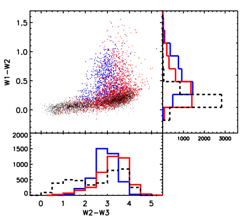
Figure 9.— The $WISE$ (W2-W3) versus (W1-W2) color diagram. Blue: type 1 AGNs; red: type 2 AGNs; black: normal galaxies. The loci of various types of objects seen here are consistent with those in Figure 12 of Wright et al. (2010) and Figure 3 of Alatalo et al. (2014). Bottom: W2-W3 histogram; right: W1-W2 histogram. Similar to Fig. 6, the distributions for type 1 AGNs and normal galaxies are scaled by a factor of 5 and 0.5, respectively.

5. Summary and Discussion

The study of the differences in environments between type 1 and type 2 AGNs can play an important role, not only in testing the unified model, but also in offering an avenue to explore the triggering/fueling processes of AGNs and the connection between supermassive black holes and their host galaxies. In this paper we have re-visited this problem by using large uniform samples selected from the SDSS, and by investigating the differences between these two types of AGNs in their clustering, host halo and host galaxy properties.

We find that, when type 1 and type 2 AGNs are matched in redshift, $M_{r}$, and $L_{\rm[O\,{\footnotesize III}]}$, the clustering strength of type 1 AGNs is almost the same as that of type 2s on large scales, but much weaker on scales smaller than about $100\,h^{-1}{\rm{kpc}}$. The clustering properties of type 2 AGNs are similar to that of normal galaxies with matched luminosities. Our results suggest that dark halos hosting type 1 AGNs, on average, have similar masses as those hosting type 2s, but that type 1s have less satellites around them. The same conclusion is reached by using galaxy groups to represent dark halos. In addition, the distribution of the satellites around type 2 AGNs are more centrally concentrated than those around type 1 AGNs. We examine various selection effects to test the reliability of our results, and find that none of the known effects can affect our results significantly.

The differences between type 1 and type 2 AGNs in their small scale clusterings provide important information about these two populations of AGNs. In the standard model, a torus-like, dusty structure is invoked to unify the two populations, and the difference in the obscuration produced by different inclination angles of the symmetric axis of the torus relative to the observational line of sight is considered to be the only reason for the discriminations of the two populations. In this case, no difference is expected between type 1s and type 2s in their environments, clearly in conflict with what we find. Our results are also different from those in some previous studies, where it was found that the two types of AGNs reside in halos of different masses but for high-luminosity quasars at higher redshift (e.g., Allevato et al. 2014; DiPompeo et al. 2014), and that there is no difference between AGNs and normal galaxies in their environments (e.g., Ebrero et al. 2009; Coil et al. 2009). It is important to note, however high-luminosity quasars at high redshift may be different from their local low luminosity counterparts, and one needs to keep this in mind when comparing the low and high redshift objects.

The fact that type 1 and type 2 AGNs have different clustering properties only on small scales suggests that galaxy interaction within dark halos may play an important role in affecting the properties of AGNs. In the unified model, the probability of a AGN to be observed as a type 2 is proportional to the covering factor of the torus, and so an AGN is more likely to be observed as a type 2 if the torus have a larger covering factor. Thus, if the environmental effects are to change the covering factor of the torus, the observed difference in the small scale clustering between type 1s and type 2s may be explained in the framework of the unified model.

The question is, of course, how the interactions on galactic ($100\,h^{-1}{\rm{kpc}}$) scales can affect the gas/dust distribution on the torus scales that is $10^{5}$ times smaller. In the co-evolution scenario for SMBHs and their host galaxies (see reviews by Kormendy & Ho 2013 and Heckman & Best 2014), AGNs are triggered by interaction with nearby galaxies (e.g., Dahari 1984; Sanders et al. 1988; Ellison et al 2011; Hong et al. 2015), which can cause cold gas/dust to lose angular momentum and flow into the central region of the interacting galaxies. As shown by high-resolution hydrodynamic simulations (e.g. Hopkins et al. 2012), when the amount of inflow gas is sufficiently large, a lopsided and eccentric inner disk can form and cause gas to move inwards to the central black hole, eventually forming a torus. This scenario is supported by recent observations (e.g., Shao et al. 2015), and consistent with our result that type 2s tend to be more strongly correlated with other galaxies so as to be more frequently affected by galaxy-galaxy interactions.

Alternatively, the interstellar medium (ISM) in the interacting galaxies may be denser and dustier, and so optically thicker in dust obscuration than in normal galaxies. Thus, a fraction of the type 2 AGNs may be obscured by galactic-scale dust distribution rather than a torus, and the difference in clustering between type 1 and type 2 AGNs may then be explained by the higher number of interacting partners in the host halos of type 2 AGNs. There are some indications for the presence of galactic-scale dust obscuration. For example, Chen et al. (2015) found that the obscuration at optical and X-ray bands in type 2 quasars is connected to the far-IR-emitting dust clouds usually located far from the central engine. In nearby low-luminosity AGNs, high resolution observations have also revealed kpc-scale dusty filamentary structures that are connected to dusty features close to the nucleus (Prieto et al. 2014). Further evidence comes from observations that Compton-thick AGNs are more likely hosted by galaxies with visible galactic dust lanes (e.g. Goulding et al. 2012; Kocevski et al. 2015). Clearly, more investigations about the dust absorption properties of type 2 AGNs are needed in order to distinguish between galactic-scale and torus obscuration.

If galaxy interaction indeed plays an important role in producing different types of AGNs, we may expect to observe some interacting signatures in the host galaxies. Unfortunately, our inspection of the host galaxies did not provide any reliable evidence for the difference between type 1 and 2 AGNs, partly due to the contamination of AGN continuum in type 1 objects. Clearly, high quality imaging data are needed to identify signatures of galaxy interactions in these objects. We should emphasize, however, that the galaxy interaction scenario discussed here is different from the popular quasar evolutionary model, in which violent mergers are assumed to be the trigger of AGNs. Moreover, the AGNs and their hosts considered here have moderate luminosities and masses, while quasar activities are probably associated with more massive galaxies. In that quasar case, a AGN may initially be heavily obscured by dust and appear as a type 2 quasar. The AGN feedback may subsequently blow away the surrounding gas and dust and evolve into an unobscured type 1 quasar. The final product of such an evolution is expected to be a red and dead early-type galaxy (Sanders et al. 1988; Hopkins et al. 2006, 2008). This is certainly not the kind of (the relatively weak) interactions we are suggesting here for the low-$z$ AGNs. Furthermore. the timescale of galaxy mergers is typically Gyr (e.g., Boylan-Kolchin et al. 2008), much longer than that of the AGN activities ($\lesssim 0.01-0.1$ Gyr) we are concerned here.

Finally, we discuss another possibility to interpret our results. It is well known that the inner structure of a dark matter halo is related to its assembly history (see e.g. Wang et al. 2011): substructures in a halo that assembled earlier tend to be destroyed by tidal stripping or have fallen onto the central objects due to dynamical friction. If, for example, type 1 AGNs are preferentially hosted by halos that formed earlier, the amounts of sub halos, which themselves host satellite galaxies and can interact with the central, may be smaller in the host halos of type 1s than in those of type 2s. This may also explain the difference in clustering between the two types of AGNs. Recently, Lim et al. (2016) used the mass ratio of the central galaxy to its host halo as an observable proxy of halo assembly time and found it is correlated with many properties of the galaxies it hosts. Moreover, halo assembly history and substructure fraction are found to depend on large scale structures (e.g. Gao et al. 2005; Wang et al. 2007), an effect usually referred to as assembly bias. Thus, this scenario based on halo assembly can be tested by studying the properties of the host halos of AGNs in detail using galaxy groups, such as those given by Yang et al. (2007).

References

- Abazajian et al. (2009) Abazajian, K. N., Adelman-McCarthy, J. K., Agüeros, M. A., et al. 2009, ApJS, 182, 543
- Adelman-McCarthy et al. (2006) Adelman-McCarthy, J. K., Agüeros, M. A., Allam, S. S., et al. 2006, ApJS, 162, 38
- Alatalo et al. (2014) Alatalo, K., Cales, S. L., Appleton, P. N., et al. 2014, ApJ, 794, L13
- Allevato et al. (2014) Allevato, V., Finoguenov, A., Civano, F., et al. 2014, ApJ, 796, 4
- Allevato et al. (2011) Allevato, V., Finoguenov, A., Cappelluti, N., et al. 2011, ApJ, 736, 99
- Antonucci (1993) Antonucci, R. 1993, ARA&A, 31, 473
- Boylan-Kolchin et al. (2008) Boylan-Kolchin, M., Ma, C.-P., & Quataert, E. 2008, MNRAS, 383, 93
- Blanton et al. (2005) Blanton, M. R., Schlegel, D. J., Strauss, M. A., et al. 2005, AJ, 129, 2562
- Chen et al. (2015) Chen, C.-T. J., Hickox, R. C., Alberts, S., et al. 2015, ApJ, 802, 50
- Chehade et al. (2016) Chehade, B., Shanks, T., Findlay, J., et al. 2016, MNRAS, 459, 1179
- Coil et al. (2007) Coil, A. L., Hennawi, J. F., Newman, J. A., Cooper, M. C., & Davis, M. 2007, ApJ, 654, 115
- Coil et al. (2009) Coil, A. L., Georgakakis, A., Newman, J. A., et al. 2009, ApJ, 701, 1484
- Croom et al. (2005) Croom, S. M., Boyle, B. J., Shanks, T., et al. 2005, MNRAS, 356, 415
- Dahari (1984) Dahari, O. 1984, AJ, 89, 966
- DiPompeo et al. (2014) DiPompeo, M. A., Myers, A. D., Hickox, R. C., Geach, J. E., & Hainline, K. N. 2014, MNRAS, 442, 3443
- DiPompeo et al. (2015) DiPompeo, M. A., Myers, A. D., Hickox, R. C., et al. 2015, MNRAS, 446, 3492
- DiPompeo et al. (2016) DiPompeo, M. A., Hickox, R. C., & Myers, A. D. 2016, MNRAS, 456, 924
- Dong et al. (2010) Dong, X.-B., Ho, L. C., Wang, J.-G., et al. 2010, ApJ, 721, L143
- Dong et al. (2012) Dong, X.-B., Ho, L. C., Yuan, W., et al. 2012, ApJ, 755, 167
- Donoso et al. (2014) Donoso, E., Yan, L., Stern, D., & Assef, R. J. 2014, ApJ, 789, 44
- Dressler (1980) Dressler, A. 1980, ApJ, 236, 351
- Dultzin-Hacyan et al. (1999) Dultzin-Hacyan, D., Krongold, Y., Fuentes-Guridi, I., & Marziani, P. 1999, ApJ, 513, L111
- Ebrero et al. (2009) Ebrero, J., Mateos, S., Stewart, G. C., Carrera, F. J., & Watson, M. G. 2009, A&A, 500, 749
- Eftekharzadeh et al. (2015) Eftekharzadeh, S., Myers, A. D., White, M., et al. 2015, MNRAS, 453, 2779
- Elitzur & Ho (2009) Elitzur, M., & Ho, L. C. 2009, ApJ, 701, L91
- Elitzur et al. (2014) Elitzur, M., Ho, L. C., & Trump, J. R. 2014, MNRAS, 438, 3340
- Ellison et al. (2011) Ellison, S. L., Patton, D. R., Mendel, J. T., & Scudder, J. M. 2011, MNRAS, 418, 2043
- Elyiv et al. (2012) Elyiv, A., Clerc, N., Plionis, M., et al. 2012, A&A, 537, A131
- Gao et al. (2005) Gao, L., Springel, V., & White, S. D. M. 2005, MNRAS, 363, L66
- Gatti et al. (2016) Gatti, M., Shankar, F., Bouillot, V., et al. 2016, MNRAS, 456, 1073
- Geach et al. (2013) Geach, J. E., Hickox, R. C., Bleem, L. E., et al. 2013, ApJ, 776, L41
- Gilli et al. (2009) Gilli, R., Zamorani, G., Miyaji, T., et al. 2009, A&A, 494, 33
- Goulding et al. (2012) Goulding, A. D., Alexander, D. M., Bauer, F. E., et al. 2012, ApJ, 755, 5
- Grogin et al. (2005) Grogin, N. A., Conselice, C. J., Chatzichristou, E., et al. 2005, ApJ, 627, L97
- Gu (2013) Gu, M. 2013, ApJ, 773, 176
- Guo et al. (2010) Guo, Q., White, S., Li, C., & Boylan-Kolchin, M. 2010, MNRAS, 404, 1111
- Hashimoto et al. (1998) Hashimoto, Y., Oemler, A., Jr., Lin, H., & Tucker, D. L. 1998, ApJ, 499, 589
- Heckman et al. (2004) Heckman, T. M., Kauffmann, G., Brinchmann, J., et al. 2004, ApJ, 613, 109
- Heckman & Best (2014) Heckman, T. M., & Best, P. N. 2014, ARA&A, 52, 589
- Hickox et al. (2009) Hickox, R. C., Jones, C., Forman, W. R., et al. 2009, ApJ, 696, 891
- Hickox et al. (2011) Hickox, R. C., Myers, A. D., Brodwin, M., et al. 2011, ApJ, 731, 117
- Hong et al. (2015) Hong, J., Im, M., Kim, M., & Ho, L. C. 2015, ApJ, 804, 34
- Hopkins et al. (2006) Hopkins, P. F., Hernquist, L., Cox, T. J., et al. 2006, ApJS, 163, 1
- Hopkins et al. (2008) Hopkins, P. F., Hernquist, L., Cox, T. J., & Kereš, D. 2008, ApJS, 175, 356-389
- Hopkins et al. (2012) Hopkins, P. F., Hayward, C. C., Narayanan, D., & Hernquist, L. 2012, MNRAS, 420, 320
- Kauffmann et al. (2003) Kauffmann, G., et al. 2003, MNRAS, 346, 1055
- Kocevski et al. (2015) Kocevski, D. D., Brightman, M., Nandra, K., et al. 2015, ApJ, 814, 104
- Kollatschny et al. (2012) Kollatschny, W., Reichstein, A., & Zetzl, M. 2012, A&A, 548, A37
- Kormendy & Ho (2013) Kormendy, J., & Ho, L. C. 2013, ARA&A, 51, 511
- Koulouridis et al. (2006) Koulouridis, E., Plionis, M., Chavushyan, V., et al. 2006, ApJ, 639, 37
- Krongold et al. (2002) Krongold, Y., Dultzin-Hacyan, D., & Marziani, P. 2002, ApJ, 572, 169
- Kraemer et al. (2011) Kraemer, S. B., Schmitt, H. R., Crenshaw, D. M., et al. 2011, ApJ, 727, 130
- Krumpe et al. (2010) Krumpe, M., Miyaji, T., & Coil, A. L. 2010, ApJ, 713, 558
- Lamastra et al. (2009) Lamastra, A., Bianchi, S., Matt, G., et al. 2009, A&A, 504, 73
- Laor (2003) Laor, A. 2003, ApJ, 590, 86
- Laurikainen & Salo (1995) Laurikainen, E., & Salo, H. 1995, A&A, 293, 683
- Lawrence (1991) Lawrence, A. 1991, MNRAS, 252, 586
- Li et al. (2006) Li, C., Kauffmann, G., Wang, L., et al. 2006, MNRAS, 373, 457
- Li et al. (2008) Li, C., Kauffmann, G., Heckman, T. M., White, S. D. M., & Jing, Y. P. 2008, MNRAS, 385, 1915
- Lietzen et al. (2009) Lietzen, H., Heinämäki, P., Nurmi, P., et al. 2009, A&A, 501, 145
- Lim et al. (2016) Lim, S. H., Mo, H. J., Wang, H., & Yang, X. 2016, MNRAS, 455, 499
- Liu et al. (2014) Liu, T., Wang, J.-X., Yang, H., Zhu, F.-F., & Zhou, Y.-Y. 2014, ApJ, 783, 106 & Primack, J. R. 2008, MNRAS, 391, 1137
- Mandelbaum et al. (2009) Mandelbaum, R., Li, C., Kauffmann, G., & White, S. D. M. 2009, MNRAS, 393, 377
- Mendez et al. (2016) Mendez, A. J., Coil, A. L., Aird, J., et al. 2016, ApJ, 821, 55
- Miyaji et al. (2011) Miyaji, T., Krumpe, M., Coil, A. L., & Aceves, H. 2011, ApJ, 726, 83
- Mo et al. (2010) Mo, H., van den Bosch, F. C., & White, S. 2010, Galaxy Formation and Evolution, by Houjun Mo , Frank van den Bosch , Simon White, Cambridge, UK: Cambridge University Press, 2010
- Myers et al. (2007) Myers, A. D., Brunner, R. J., Nichol, R. C., et al. 2007, ApJ, 658, 85
- Nandra et al. (2007) Nandra, K., Georgakakis, A., Willmer, C. N. A., et al. 2007, ApJ, 660, L11
- Netzer et al. (2006) Netzer, H., Mainieri, V., Rosati, P., & Trakhtenbrot, B. 2006, A&A, 453, 525
- Netzer (2015) Netzer, H. 2015, ARA&A, 53, 365
- Padmanabhan et al. (2009) Padmanabhan, N., White, M., Norberg, P., & Porciani, C. 2009, MNRAS, 397, 1862
- Pasquali et al. (2009) Pasquali, A., van den Bosch, F. C., Mo, H. J., Yang, X., & Somerville, R. 2009, MNRAS, 394, 38
- Porciani et al. (2004) Porciani, C., Magliocchetti, M., & Norberg, P. 2004, MNRAS, 355, 1010
- Prieto et al. (2014) Prieto, M. A., Mezcua, M., Fernández-Ontiveros, J. A., & Schartmann, M. 2014, MNRAS, 442, 2145
- Reines & Volonteri (2015) Reines, A. E., & Volonteri, M. 2015, ApJ, 813, 82
- Richardson et al. (2012) Richardson, J., Zheng, Z., Chatterjee, S., Nagai, D., & Shen, Y. 2012, ApJ, 755, 30
- Ross et al. (2009) Ross, N. P., Shen, Y., Strauss, M. A., et al. 2009, ApJ, 697, 1634
- Salim et al. (2007) Salim, S., Rich, R. M., Charlot, S., et al. 2007, ApJS, 173, 267
- Sanders et al. (1988) Sanders, D. B., Soifer, B. T., Elias, J. H., et al. 1988, ApJ, 325, 74
- Shaver (1984) Shaver, P. A. 1984, A&A, 136, L9
- Schmitt (2001) Schmitt, H. R. 2001, AJ, 122, 2243
- Schlegel et al. (1998) Schlegel, D. J., Finkbeiner, D. P., & Davis, M. 1998, ApJ, 500, 525
- Serber et al. (2006) Serber, W., Bahcall, N., Ménard, B., & Richards, G. 2006, ApJ, 643, 68
- Shao et al. (2015) Shao, L., Li, C., Kauffmann, G., & Wang, J. 2015, MNRAS, 448, L72
- Shen et al. (2007) Shen, Y., Strauss, M. A., Oguri, M., et al. 2007, AJ, 133, 2222
- Shen et al. (2009) Shen, Y., Strauss, M. A., Ross, N. P., et al. 2009, ApJ, 697, 1656
- Shen et al. (2013) Shen, Y., McBride, C. K., White, M., et al. 2013, ApJ, 778, 98
- Strand et al. (2008) Strand, N. E., Brunner, R. J., & Myers, A. D. 2008, ApJ, 688, 180
- Vale & Ostriker (2004) Vale, A., & Ostriker, J. P. 2004, MNRAS, 353, 189
- Villarroel & Korn (2014) Villarroel, B., & Korn, A. J. 2014, Nature Physics, 10, 417
- Wang et al. (2007) Wang, H. Y., Mo, H. J., & Jing, Y. P. 2007, MNRAS, 375, 633
- Wang et al. (2011) Wang, H., Mo, H. J., Jing, Y. P., Yang, X., & Wang, Y. 2011, MNRAS, 413, 1973
- Wake et al. (2004) Wake, D. A., Miller, C. J., Di Matteo, T., et al. 2004, ApJ, 610, L85
- White & Rees (1978) White, S. D. M., & Rees, M. J. 1978, MNRAS, 183, 341
- Wright et al. (2010) Wright, E. L., Eisenhardt, P. R. M., Mainzer, A. K., et al. 2010, AJ, 140, 1868
- Yang et al. (2003) Yang, X., Mo, H. J., & van den Bosch, F. C. 2003, MNRAS, 339, 1057
- Yang et al. (2005) Yang, X., Mo, H. J., van den Bosch, F. C., & Jing, Y. P. 2005, MNRAS, 356, 1293
- Yang et al. (2007) Yang, X., Mo, H. J., van den Bosch, F. C., et al. 2007, ApJ, 671, 153
- Zehavi et al. (2002) Zehavi, I., Blanton, M. R., Frieman, J. A., et al. 2002, ApJ, 571, 172
- Zehavi et al. (2011) Zehavi, I., Zheng, Z., Weinberg, D. H., et al. 2011, ApJ, 736, 59
- Zhang et al. (2008) Zhang, K., Wang, T., Dong, X., & Lu, H. 2008, ApJ, 685, L109
- Zhang et al. (2013) Zhang, S., Wang, T., Wang, H., & Zhou, H. 2013, ApJ, 773, 175